A Survey on Oversmoothing in Graph Neural Networks

Abstract

Node features of graph neural networks (GNNs) tend to become more similar with the increase of the network depth. This effect is known as over-smoothing, which we axiomatically define as the exponential convergence of suitable similarity measures on the node features. Our definition unifies previous approaches and gives rise to new quantitative measures of over-smoothing. Moreover, we empirically demonstrate this behavior for several over-smoothing measures on different graphs (small-, medium-, and large-scale). We also review several approaches for mitigating over-smoothing and empirically test their effectiveness on real-world graph datasets. Through illustrative examples, we demonstrate that mitigating over-smoothing is a necessary but not sufficient condition for building deep GNNs that are expressive on a wide range of graph learning tasks. Finally, we extend our definition of over-smoothing to the rapidly emerging field of continuous-time GNNs.

1 Introduction

Graph Neural Networks (GNNs) (Sperduti, 1994; Goller & Kuchler, 1996; Sperduti & Starita, 1997; Frasconi et al., 1998; Gori et al., 2005; Scarselli et al., 2008; Bruna et al., 2014; Defferrard et al., 2016; Kipf & Welling, 2017; Monti et al., 2017; Gilmer et al., 2017) have emerged as a powerful tool for learning on relational and interaction data. These models have been successfully applied on a variety of different tasks, e.g. in computer vision and graphics Monti et al. (2017), recommender systems Ying et al. (2018), transportation Derrow-Pinion et al. (2021), computational chemistry (Gilmer et al., 2017), drug discovery Gaudelet et al. (2021), particle physics (Shlomi et al., 2020), and analysis of social networks (see Zhou et al. (2019); Bronstein et al. (2021) for additional applications).

The number of layers in a neural network (referred to as “depth” and giving the name to the entire field of “deep learning”) is often considered to be crucial for its performance on real-world tasks. For example, convolutional neural networks (CNNs) used in computer vision, often use tens or even hundreds of layers. In contrast, most GNNs encountered in applications are relatively shallow and often have just few layers. This is related to several issues impairing the performance of deep GNNs in realistic graph-learning settings: graph bottlenecks (Alon & Yahav, 2021), over-squashing (Topping et al., 2021; Deac et al., 2022), and over-smoothing (Li et al., 2018; Nt & Maehara, 2019; Oono & Suzuki, 2020). In this article we focus on the over-smoothing phenomenon, which loosely refers to the exponential convergence of all node features towards the same constant value as the number of layers in the GNN increases. While it has been shown that small amounts of smoothing are desirable for regression and classification tasks (Keriven, 2022), excessive smoothing (or ‘over-smoothing’) results in convergence to a non-informative limit. Besides being a key limitation in the development of deep multi-layer GNNs, over-smoothing can also severely impact the ability of GNNs to handle heterophilic graphs (Zhu et al., 2020), in which node labels tend to differ from the labels of the neighbors and thus long-term interactions have to be learned.

Recent literature has focused on precisely defining over-smoothing through measures of node feature similarities such as the the graph Dirichlet (Rusch et al., 2022; Cai & Wang, 2020; Zhao & Akoglu, 2019; Zhou et al., 2021a), cosine similarity (Chen et al., 2020a), and other related similarity scores (Zhou et al., 2020). With the abundance of such measures, however, there is currently still a conceptual gap in a general definition of over-smoothing that would provide a unification of existing approaches. Moreover, previous work mostly measures the similarity of node features and does not explicitly consider the rate of convergence of over-smoothing measures with respect to an increasing number of GNN layers.

In this article, we aim to unify several recent approaches and define over-smoothing in a formal and tractable manner through an axiomatic construction. Through our definition, we rule out problematic measures such as the Mean Average Distance that does not provide a sufficient condition for over-smoothing. We then review several approaches to mitigate over-smoothing and provide their extensive empirical evaluation. These empirical studies lead to the insight that meaningfully solving over-smoothing in deep GNNs is more elaborate than simply forcing the node features not to converge towards the same node value when the number of layers is increased. Rather, there needs to be a subtle balance between the expressive power of the deep GNN and its ability to preserve the diversity of node features in the graph. Finally, we extend our definition to the rapidly emerging sub-field of continuous-time GNNs (Chamberlain et al., 2021a, b; Rusch et al., 2022, 2023; Bodnar et al., 2022; Di Giovanni et al., 2022).

2 Definition of over-smoothing

Let $\mathcal{G}=(\mathcal{V},\mathcal{E}\subseteq\mathcal{V}\times\mathcal{V})$ be an undirected graph with $|\mathcal{V}|=v$ nodes and $|\mathcal{E}|=e$ edges (unordered pairs of nodes $\{i,j\}$ denoted $i\sim j$). The $1$-neighborhood of a node $i$ is denoted $\mathcal{N}_{i}=\{j\in\mathcal{V}:i\sim j\}$. Furthermore, each node $i$ is endowed with an $m$-dimensional feature vector $\mathbf{X}_{i}$; the node features are arranged into a $v\times m$ matrix ${\bf X}=({\bf X}_{ik})$ with $i=1,\ldots,v$ and $k=1,\ldots,m$.

Message-Passing GNN (MPNN) updates the node features by performing several iterations of the form,

$${\bf X}^{n}=\sigma({\bf F}_{\theta^{n}}({\bf X}^{n-1},\mathcal{G})),\quad\forall n=1,\dots,N,$$ (1)

where ${\bf F}_{\theta^{n}}$ is a learnable function with parameters $\theta^{n}$, ${\bf X}^{n}\in\mathbb{R}^{v\times m_{n}}$ are the $m$-dimensional hidden node features, and $\sigma$ is an element-wise non-linear activation function. Here, $n\geq 1$ denotes the $n$-th layer with $n=0$ being the input layer and $N$ the total number of layers (depth). In particular, we consider local (1-neighborhood) coupling of the form $(\mathbf{F}(\mathbf{X},\mathcal{G}))_{i}=\mathbf{F}(\mathbf{X}_{i},\mathbf{X}_{j\in\mathcal{N}_{i}})$ operating on the multiset of 1-neighbors of each node. Examples of such functions used in the graph machine learning literature (Bronstein et al., 2021) include graph convolutions (Kipf & Welling, 2017) and attentional message passing (Velickovic et al., 2018).

There exist a variety of different approaches to quantify over-smoothing in deep GNNs, e.g. measures based on the Dirichlet energy on graphs (Rusch et al., 2022; Cai & Wang, 2020; Zhao & Akoglu, 2019; Zhou et al., 2021a), as well as measures based on the mean-average distance (MAD) (Chen et al., 2020a; Zhou et al., 2020), and references therein. However, most previous approaches lack a formal definition of over-smoothing as well as provide approaches to measure over-smoothing which are not sufficient to quantify this issue. Thus, the aim of this survey is to establish a unified, rigorous, and tractable definition of over-smoothing, which we provide in the following. [Over-smoothing] Let $\mathcal{G}$ be an undirected, connected graph and ${\bf X}^{n}\in\mathbb{R}^{v\times m}$ denote the $n$-th layer hidden features of an $N$-layer GNN defined on $\mathcal{G}$. Moreover, we call $\mu:\mathbb{R}^{v\times m}\longrightarrow\mathbb{R}_{\geq 0}$ a node-similarity measure if it satisfies the following axioms:

1. $\exists{\bf c}\in\mathbb{R}^{m}$ with ${\bf X}_{i}={\bf c}$ for all nodes $i\in\mathcal{V}$ $\Leftrightarrow$ $\mu({\bf X})=0$,  for ${\bf X}\in\mathbb{R}^{v\times m}$

2. $\mu({\bf X}+{\bf Y})\leq\mu({\bf X})+\mu({\bf Y})$,  for all ${\bf X},{\bf Y}\in\mathbb{R}^{v\times m}$

We then define over-smoothing with respect to $\mu$ as the layer-wise exponential convergence of the node-similarity measure $\mu$ to zero, i.e.,

1. $\mu({\bf X}^{n})\leq C_{1}e^{-C_{2}n}$, for $n=0,\dots,N$ with some constants $C_{1},C_{2}>0$.

Note that without loss of generality we assume that the node-similarity measure $\mu$ converges to zero (any node-similarity measure that converges towards a non-zero constant can easily be recast). Further remarks about Definition 2 are in order.

Remark 2.1.

Condition 1 in Definition 2 simply formalizes the widely accepted notion that over-smoothing is caused by node features converging to a constant node vector whereas condition 3 provides a more stringent, quantitative measure of this convergence. Note that the triangle inequality or subadditivity (condition 2) rules out degenerate choices of similarity measures.

Remark 2.2.

Definition 2 only considers the case of connected graphs. However, this definition can be directly generalized to disconnected graphs, where we apply a node-similarity measure $\mu_{S}$ on every connected component $S\subseteq\mathcal{V}$, and define the global similarity measure as the sum of the node-similarity measures on each connected component, i.e., $\mu=\sum_{S}\mu_{S}$. This way we ensure to cover the case of different connected components converging to different constant node values.

3 Over-smoothing measures

Existing approaches to measure over-smoothing in deep GNNs have mainly been based on concept of Dirichlet energy on graphs,

$$\mathcal{E}({\bf X}^{n})=\frac{1}{v}\sum_{i\in\mathcal{V}}\sum_{j\in\mathcal{N}_{i}}\|{\bf X}^{n}_{i}-{\bf X}^{n}_{j}\|^{2}_{2},$$ (2)

(note that instead of normalizing by $1/v$ we can equivalently normalize the terms inside the norm based on the node degrees $d_{i}$, i.e. $\|\frac{{\bf X}^{n}_{i}}{\sqrt{1+d_{i}}}-\frac{{\bf X}^{n}_{j}}{\sqrt{1+d_{j}}}\|^{2}_{2}$). It is straightforward to check that the measure,

$$\mu({\bf X}^{n})=\sqrt{\mathcal{E}({\bf X}^{n})},$$ (3)

satisfies the conditions 1 and 2 in the definition 2 and thus, constitutes a bona fide node-similarity measure. Note that in the remainder of this article, we will refer to the square root of the Dirichlet energy simply as the Dirichlet energy.

In the literature, Mean Average Distance (MAD),

$$\mu({\bf X}^{n})=\frac{1}{v}\sum_{i\in\mathcal{V}}\sum_{j\in\mathcal{N}_{i}}1-\frac{{{\bf X}^{n}_{i}}^{\top}{\bf X}^{n}_{j}}{\|{\bf X}^{n}_{i}\|\|{\bf X}^{n}_{j}\|}.$$ (4)

has often been suggested as a measure of over-smoothing. We see that in contrast to the Dirichlet energy, MAD is not a node-similarity measure, as it does not fulfill condition 1 nor condition 2 of the over-smoothing definition 2. In fact, MAD is always zero in the scalar case, where all node features share the same sign for each feature dimension. This makes MAD a very problematic measure for over-smoothing as $\mu({\bf X})=0$ does not represent a sufficient condition for over-smoothing to happen. However, as we will see in the subsequent section, in the multi-dimensional case ($m>1$) MAD does converge exponentially to zero for increasing number of layers if the GNN over-smooths and thus fulfills condition 3 of the over-smoothing definition 2. Therefore, we conclude that under careful considerations of the specific use-case, MAD may be used as a measure for over-smoothing. However, since the Dirichlet energy fulfills all three conditions of Definition 2 and is numerically more stable to compute, it should always be favored over MAD.

It is natural to ask if there exist other measures that constitute a node-similarity measure as of Definition 2 and can thus be used to define over-smoothing. While the Dirichlet energy denotes a canonical choice in this context, there are other measures that can be used. For instance, instead of basing the Dirichlet energy in (2) on the $L^{2}$ norm, any other $L^{p}$-norm ($p>1$) can be used.

3.1 Empirical evaluation of different measures for over-smoothing

Rusch et al. (2022) have empirically demonstrated the qualitative behavior described in Definition 2 on a $10\times 10$ regular 2-dimensional grid with one-dimensional uniform random (hidden) node features. We extend this empirical study in two directions, first to higher dimensional node features and also to real-world graphs, namely Texas (Pei et al., 2020), Cora (McCallum et al., 2000), and Cornell5 (Facebook 100 dataset). Note that as mentioned above, the extension to higher dimensional node features is necessary in order to empirically evaluate MAD, as MAD is zero for any one-dimensional node features sharing the same sign.

Since we are interested only in the dynamics of the Dirichlet energy and MAD associated with the propagation of node features through different GNN architectures, we omit the original input node features of the real-world graph dataset Cora and exchange them for standard normal random variables, i.e., ${\bf X}_{jk}\sim\mathcal{N}(0,1)$ for all nodes $j$ and every feature $k$. In Fig. 1 we set the input and hidden dimension of the node features to $128$ and plot the (logarithm of) the Dirichlet energy (2) and MAD (4)) of each layer’s node features with respect to the (logarithm of) layer number for three popular GNN models, i.e., GCN, GAT and the GraphSAGE architecture of Hamilton et al. (2017). We can see that all three GNN architectures over-smooth, with both layer-wise measures converging exponentially fast to zero for increasing number of layers. Moreover, we observe that this behavior is not just restricted to the structured and regular grid dataset of Rusch et al. (2022), but the same behavior (i.e., exponential convergence of the measures with respect to increasing number of layers) can be seen on all the three real-world graph datasets considered here.

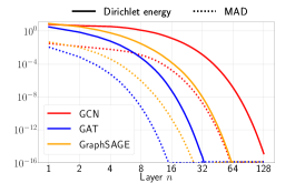
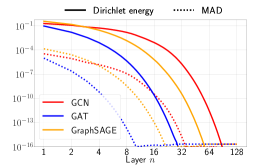
Figure 1: Dirichlet energy and Mean Average Distance (MAD) of layer-wise node features ${\bf X}^{n}$ propagated through a GAT, GCN and GraphSAGE for three different graph datasets, (left) small-scale Texas graph, (middle) medium-scale Cora citation network, (right) large-scale Facebook network (Cornell5).

It is important to emphasize the importance of the exponential convergence of the layer-wise over-smoothing measure $\mu$ to zero in Definition 2. Algebraic convergence is not sufficient for the GNN to suffer from over-smoothing. This can be seen in Fig. 1, where for instance the Dirichlet energy of GCN, GraphSAGE and GAT reach machine-precision zero after a maximum of $64$ layers, while for instance a linear convergence of the Dirichlet energy would still have a Dirichlet energy of around $1$ for an initial energy of around $100$, even after $128$ hidden layers.

4 Reducing over-smoothing

4.1 Methods

Several methods to mitigate (or at least reduce) the effect of over-smoothing in deep GNNs have recently been proposed. While we do not discuss each individual approach, we highlight several recent methods in this context, all of which can be classified into one of the following classes.

Normalization and Regularization

A proven way to reduce the over-smoothing effect in deep GNNs is to regularize the training procedure. This can be done either explicitly by penalizing deviations of over-smoothing measures during training or implicitly by normalizing the node feature embeddings and by adding noise to the optimization process. An example of explicit regularization techniques can be found in Energetic Graph Neural Networks (EGNNs) (Zhou et al., 2021a), where the authors measure over-smoothing using the Dirichlet energy and propose to optimize a GNN within a constrained range of the underlying layer-wise Dirichlet energy. DropEdge (Rong et al., 2020) on the other hand represents an example of implicit regularization by adding noise to the optimization process. This is done by randomly dropping edges of the underlying graph during training. Graph DropConnect (GDC) (Hasanzadeh et al., 2020) generalizes this approach by allowing the GNNs to draw different random masks for each channel and edge independently. Another example of implicit regularization is PairNorm (Zhao & Akoglu, 2019), where the pairwise distances are set to be constant throughout every layer in the deep GNN. This is obtained by performing the following normalization on the node features ${\bf X}$ after each GNN layer,

$$\hat{{\bf X}}_{i} ={\bf X}_{i}-\frac{1}{v}\sum_{j=1}^{v}{\bf X}_{j},$$ (5)

$${\bf X}_{i} =\frac{s\hat{{\bf X}}_{i}}{\sqrt{\frac{1}{v}\sum_{j=1}^{v}\|\hat{{\bf X}}_{j}\|_{2}^{2}}},$$

where $s>0$ is a hyperparameter. Similarly, Zhou et al. (2020) have suggested to normalize within groups of the same labeled nodes, leading to Differentiable Group Normalization (DGN). Moreover, Zhou et al. (2021b) have suggested to node-wise normalize each feature vector, yielding NodeNorm.

Change of GNN dynamics

A rapidly emerging strategy to mitigate over-smoothing for deep GNNs is by qualitatively changing the (discrete or continuous) dynamics of the message-passing propagation. A recent example is the use of non-linear oscillators which are coupled through the graph structure yielding Graph-Coupled Oscillator Network (GraphCON) (Rusch et al., 2022),

$${\bf Y}^{n} ={\bf Y}^{n-1}+{\Delta t}[\sigma({\bf F}_{\theta^{n}}({\bf X}^{n-1},\mathcal{G}))-\gamma{\bf X}^{n-1}-\alpha{\bf Y}^{n-1}],$$ (6)

$${\bf X}^{n} ={\bf X}^{n-1}+{\Delta t}{\bf Y}^{n},$$

where ${\bf Y}^{n}$ are auxiliary node features and $\Delta t>0$ denotes the time-step (usually set to $\Delta t=1$). The idea of this work is to exchange the diffusion-like dynamics of GCNs (and its variants) to that of non-linear oscillators, which can provably be guaranteed to have a Dirichlet energy that does not exponentially vanish (as of Definition 2). A similar approach has been taken in Eliasof et al. (2021), where the dynamics of a deep GCN is modelled as a wave-type partial differential equation (PDE) on graphs, yielding PDE-GCN. Another approach inspired by physical systems is Allen-Cahn Message Passing (ACMP) (Wang et al., 2022), where the dynamics is constructed based on the Allen-Cahn equation modeling interacting particle system with attractive and repulsive forces. A related effort is the Gradient Flow Framework (GRAFF) (Di Giovanni et al., 2022), where the proposed GNN framework can be interpreted as attractive respectively repulsive forces between adjacent features.

A recent example in this direction, that is not directly inspired by physical systems, is that of Gradient Gating (G²) (Rusch et al., 2023), where a learnable node-wise early-stopping mechanism is realized through a gating function leveraging the graph-gradient,

$$\hat{\boldsymbol{\tau}}^{n} ={\sigma}(\hat{{\bf F}}_{\hat{\theta}^{n}}({\bf X}^{n-1},\mathcal{G})),$$ (7)

$$\boldsymbol{\tau}^{n}_{ik} =\tanh\left(\sum_{j\in\mathcal{N}_{i}}|\hat{\boldsymbol{\tau}}^{n}_{jk}-\hat{\boldsymbol{\tau}}^{n}_{ik}|^{p}\right),$$

$${\bf X}^{n} =(1-\boldsymbol{\tau}^{n})\odot{\bf X}^{n-1}+\boldsymbol{\tau}^{n}\odot\sigma({\bf F}_{\theta^{n}}({\bf X}^{n-1},\mathcal{G})),$$

with $p\geq 0$. This mechanism slows down the message-passing propagation corresponding to each individual node (and each individual channel) as $\hat{\boldsymbol{\tau}}^{n}_{ij}$ goes to zero before local over-smoothing occurs in the $j$-th channel on a node $i$.

Residual connections

Motivated by the success of residual neural networks (ResNets) (He et al., 2016) in conventional deep learning, there has been many suggestions of adding residual connections to deep GNNs. An early example includes Li et al. (2019), where the authors equip a GNN with a residual connection He et al. (2016), i.e.,

$${\bf X}^{n}={\bf X}^{n-1}+{\bf F}_{\theta^{n}}({\bf X}^{n-1},\mathcal{G}).$$ (8)

By instantiating the GNN in (8) with a GCN, this leads to major improvements over competing methods. Another example is GCNII (Chen et al., 2020b) where a scaled residual connection of the initial node features is added to every layer of a GCN,

$${\bf X}^{n}=\sigma\left[\left((1-\alpha_{n})\hat{{\bf D}}^{-\frac{1}{2}}\hat{{\bf A}}\hat{{\bf D}}^{-\frac{1}{2}}{\bf X}^{n-1}+\alpha_{n}{\bf X}^{0}\right)\left((1-\beta_{n})\mathrm{I}+\beta_{n}{\bf W}^{n}\right)\right],$$ (9)

where $\alpha_{n},\beta_{n}\in[0,1]$ are fixed hyperparameters for all $n=1,\dots,N$. This allows for constructing very deep GCNs, outperforming competing methods on several benchmark tasks. Similar approaches aggregate not just the initial node features but all node features of every layer of a deep GNN at the final layer. Examples of such models include Jumping Knowledge Networks (JKNets) (Xu et al., 2018) and Deep Adaptive Graph Neural Networks (DAGNNs) (Liu et al., 2020)

4.2 Empirical evaluation

In order to evaluate the effectiveness of the different methods that have been suggested to mitigate over-smoothing in deep GNNs, we follow the experimental set-up of section 3. To this end, we choose two representative methods of each of the different strategies to overcome over-smoothing, namely DropEdge and PairNorm as representatives from “normalization and regularization” strategies, GraphCON and G² from “change of GNN dynamics”, and Residual GCN (Res-GCN) and GCNII from “residual connections”. We consider the same three different graphs as in section 3, namely small-scale Texas, medium-scale Cora and larger-scale Cornell5 graph. Since we are only interested in the qualitative behavior of the different methods, we fix one node-similarity measure, namely the Dirichlet energy. Thereby, we can see in Fig. 2 that DropEdge-GCN and Res-GCN suffer from an exponential convergence of the layer-wise Dirichlet energy to zero (and thus from over-smoothing) on all three graphs. In contrast to that, all other methods we consider here mitigate over-smoothing by keeping the layer-wise Dirichlet energy approximately constant.

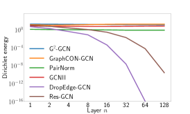
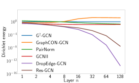
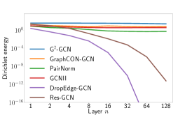
Figure 2: Layer-wise Dirichlet energy of hidden node features propagated through G²-GCN, GraphCON-GCN, PairNorm, GCNII, DropEdge-GCN and Res-GCN on three different graphs, i.e., (left) small-scale Texas graph, (middle) medium-scale Cora citation network, (right) large-scale Facebook (Cornell5) network.

5 Risk of sacrificing expressivity to mitigate over-smoothing

Since several of the previously suggested methods designed to mitigate over-smoothing successfully prevent the layer-wise Dirichlet energy (and other node-similarity measures) from converging exponentially fast to zero, it is natural to ask if this is already sufficient to construct (possibly very) deep GNNs which also efficiently solve the learning task at hand. To answer this question, we start by constructing a deep GCN which keeps the Dirichlet energy constant while at the same time its performance on a learning task is as poor as a standard deep multi-layer GCN.

It turns out that simply adding a bias vector to a deep GCN with shared parameters among layers, i.e.,

$${\bf X}^{n}=\sigma(\hat{{\bf D}}^{-\frac{1}{2}}\hat{{\bf A}}\hat{{\bf D}}^{-\frac{1}{2}}{\bf X}^{n-1}{\bf W}+{\bf b}),\quad\forall n=1,\dots,N,$$

with weights ${\bf W}\in\mathbb{R}^{m\times m}$ and bias ${\bf b}\in\mathbb{R}^{m}$, is sufficient for the optimizer to keep the resulting layer-wise Dirichlet energy of the model approximately constant. This can be seen in Fig. 3 where the layer-wise Dirichlet energy is shown (among others) for a standard GCN as well as a GCN with an additional bias term after training on the Cora graph dataset in the fully supervised setting. We observe that while the Dirichlet energy converges exponentially fast to zero for the standard GCN, simply adding a bias term results in an approximately constant layer-wise Dirichlet energy. Moreover, Fig. 3 shows the test accuracy of the same models for different number of layers. We can see that both the standard GCN as well as the GCN with bias vector suffer from a significant decrease of performance for increasing number of layers. Interestingly, while GCN with bias keeps the Dirichlet energy perfectly constant and GCN without bias exhibits a Dirichlet energy converging exponentially fast to zero, both models suffer similarly from drastic impairment of performance (in terms of test accuracy) for increasing number of layers. We thus observe that simply constructing a deep GNN that keeps the node-similarity measure constant (around $1$) is not sufficient in order to successfully construct deep GNNs.

This observation is further supported in Fig. 3 by looking at the Dirichlet energy of the PairNorm method which behaves similarly to the Dirichlet energy of GCN with bias, i.e., approximately constant around $1$. However, the performance in terms of test accuracy on the Cora graph dataset drops exponentially after using more than $32$ layers. Interestingly, G²-GCN exhibits an approximately constant layer-wise Dirichlet energy and at the same time does not decrease its performance by increasing number of layers. In fact the performance of G²-GCN increases slightly by increasing number of layers.

Therefore, we argue that solving the over-smoothing issue defined in Definition 2 is necessary in order to construct well performing deep GNNs. Otherwise the network is not able to learn any meaningful function defined on the graph. However, as can be seen from this experiment it is not sufficient. Therefore, based on this experiment we conclude that a major pitfall in designing deep GNNs that mitigate over-smoothing is to sacrifice the expressive power of the GNN only to keep the node-similarity measure approximately constant. In fact, based on our experiments, only G² (among the considered models here) fully mitigates the over-smoothing issue by keeping the node-similarity measure approximately constant, while at the same time increasing its expressive power for increasing number of layers.

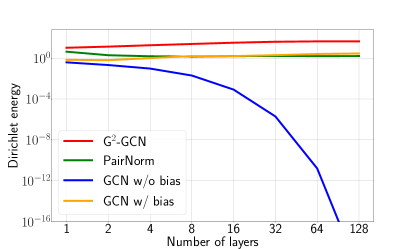
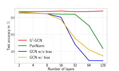
Figure 3: Trained G²-GCN, PairNorm, GCN with bias and GCN without bias on the fully-supervised Cora graph dataset using the pre-defined $10$ splits from Pei et al. (2020), showing two different measures for increasing number of layers ranging from $1$ to $128$: (left) Dirichlet energy of the layer-wise node features, (right) test accuracies.

6 Extension to continuous-time GNNs

A rapidly growing sub-field of graph representation learning deals with GNNs that are continuous in depth. This is performed by formulating the message-passing propagation in terms of graph dynamical systems modelled by (neural (Chen et al., 2018)) Ordinary Differential Equations (ODEs) or Partial Differential Equations (PDEs), i.e., message-passing framework (1), where the forward propagation is modeled by a differential equation:

$${\bf X}^{\prime}(t)=\sigma({\bf F}_{\theta}({\bf X}(t),\mathcal{G})),$$ (10)

with ${\bf X}(t)$ referring to the node features at time $t\geq 0$. Different choices of the vector field (i.e., right-hand side of (10)) yields different architectures. Moreover, we note that the right-hand side in (10) can potentially arise from a discretization of a differential operator defined on a graph leading to a PDE-inspired architecture. We refer to this class of graph-learning models as continuous-time GNNs. Early examples of continuous-time GNNs include Graph Neural Ordinary Differential Equations (GDEs) (Poli et al., 2019) and Continuous Graph Neural Networks (CGNN) (Xhonneux et al., 2020). More recent examples include Graph-Coupled Oscillator Networks (GraphCON) (Rusch et al., 2022), Graph Neural Diffusion (GRAND) (Chamberlain et al., 2021a), Beltrami Neural Diffusion (BLEND) (Chamberlain et al., 2021b), Neural Sheaf Diffusion (NSD) (Bodnar et al., 2022), and Gradient Glow Framework (GRAFF) (Di Giovanni et al., 2022). Based on this framework, we can easily extend our definition of over-smoothing 2 to continuous-time GNNs, by defining over-smoothing as the exponential convergence in time of a node-similarity measure. More concretely, we define it as follows. [Continuous-time over-smoothing] Let $\mathcal{G}$ be an undirected, connected graph and ${\bf X}(t)\in\mathbb{R}^{v\times m}$ denote the hidden node features of a continuous-time GNN (10) at time $t\geq 0$ defined on $\mathcal{G}$. Moreover, $\mu$ is a node-similarity measure as of Definition 2. We then define over-smoothing with respect to $\mu$ as the exponential convergence in time of the node-similarity measure $\mu$ to zero, i.e.,

1. $\mu({\bf X}(t))\leq C_{1}e^{-C_{2}t}$, for $t\geq 0$ with some constants $C_{1},C_{2}>0$.

7 Conclusion

Stacking multiple message-passing layers (i.e., a deep GNN) is necessary in order to effectively process information on relational data where the underlying computational graph exhibits (higher-order) long-range interactions. This is of particular importance for learning heterophilic graph data, where node labels may differ significantly from those of their neighbors. Besides several other identified problems (e.g., over-squashing, exploding and vanishing gradients problem), the over-smoothing issue denotes a central challenge in constructing deep GNNs.

Since previous work has measured over-smoothing in various ways, we unify those approaches by providing an axiomatic definition of over-smoothing through the layer-wise exponential convergence of similarity measures on the node features. Moreover, we review recent measures for over-smoothing and, based on our definition, rule out the commonly used MAD in the context of measuring over-smoothing. Additionally, we test the qualitative behavior of those measures on three different graph datasets, i.e., small-scale Texas graph, medium-scale Cora graph, and large-scale Cornell5 graph, and observe an exponential convergence to zero of all measures for standard GNN models (i.e., GCN, GAT, and GraphSAGE). We further review prominent approaches to mitigate over-smoothing and empirically test whether these methods are able to successfully overcome over-smoothing by plotting the layer-wise Dirichlet energy on different graph datasets.

We conclude by highlighting the need for balancing the ability of models to mitigate over-smoothing, but without sacrificing the expressive power of the underlying deep GNN. This phenomenon was illustrated by the example of a simple deep GCN with shared parameters among all layers as well as a bias, where the optimizer rapidly finds a state of parameters during training that leads to a mitigation of over-smoothing (i.e., approximately constant Dirichlet energy). However, in terms of performance (or accuracy) on the Cora graph-learning task, this model fails to outperform its underlying baseline (i.e., same GCN model without a bias) which suffers from over-smoothing. This behavior is further observed in other methods that are particularly designed to mitigate over-smoothing, where the over-smoothing measure remains approximately constant but at the same time the accuracy of the model drops significantly for increasing number of layers. However, we also want to highlight that there exist methods that are able to mitigate over-smoothing while at the same time maintaining its expressive power on our task, i.e., G². We thus conclude that mitigating over-smoothing is only a necessary condition, among many others, for building deep GNNs, while a particular focus in designing methods in this context has to be on the maintenance or potential enhancement of the expressive power of the underlying model.

References

- Alon & Yahav (2021) Uri Alon and Eran Yahav. On the bottleneck of graph neural networks and its practical implications. In ICML, 2021.
- Bodnar et al. (2022) Cristian Bodnar, Francesco Di Giovanni, Benjamin Paul Chamberlain, Pietro Liò, and Michael M Bronstein. Neural sheaf diffusion: A topological perspective on heterophily and oversmoothing in gnns. arXiv preprint arXiv:2202.04579, 2022.
- Bronstein et al. (2021) Michael M Bronstein, Joan Bruna, Taco Cohen, and Petar Veličković. Geometric deep learning: Grids, groups, graphs, geodesics, and gauges. arXiv:2104.13478, 2021.
- Bruna et al. (2014) Joan Bruna, Wojciech Zaremba, Arthur Szlam, and Yann LeCun. Spectral networks and locally connected networks on graphs. In 2nd International Conference on Learning Representations, ICLR 2014, 2014.
- Cai & Wang (2020) Chen Cai and Yusu Wang. A note on over-smoothing for graph neural networks. arXiv preprint arXiv:2006.13318, 2020.
- Chamberlain et al. (2021a) Ben Chamberlain, James Rowbottom, Maria I. Gorinova, Michael M. Bronstein, Stefan Webb, and Emanuele Rossi. GRAND: graph neural diffusion. In Proceedings of the 38th International Conference on Machine Learning, volume 139, pp. 1407–1418. PMLR, 2021a.
- Chamberlain et al. (2021b) Benjamin Chamberlain, James Rowbottom, Davide Eynard, Francesco Di Giovanni, Xiaowen Dong, and Michael Bronstein. Beltrami flow and neural diffusion on graphs. In NeurIPS, 2021b.
- Chen et al. (2020a) Deli Chen, Yankai Lin, Wei Li, Peng Li, Jie Zhou, and Xu Sun. Measuring and relieving the over-smoothing problem for graph neural networks from the topological view. In Proceedings of the AAAI Conference on Artificial Intelligence, volume 34, pp. 3438–3445, 2020a.
- Chen et al. (2020b) Ming Chen, Zhewei Wei, Zengfeng Huang, Bolin Ding, and Yaliang Li. Simple and deep graph convolutional networks. In International Conference on Machine Learning, pp. 1725–1735. PMLR, 2020b.
- Chen et al. (2018) Ricky TQ Chen, Yulia Rubanova, Jesse Bettencourt, and David K Duvenaud. Neural ordinary differential equations. Advances in neural information processing systems, 31, 2018.
- Deac et al. (2022) Andreea Deac, Marc Lackenby, and Petar Veličković. Expander graph propagation. arXiv preprint arXiv:2210.02997, 2022.
- Defferrard et al. (2016) Michaël Defferrard, Xavier Bresson, and Pierre Vandergheynst. Convolutional neural networks on graphs with fast localized spectral filtering. Advances in neural information processing systems, 29:3844–3852, 2016.
- Derrow-Pinion et al. (2021) Austin Derrow-Pinion, Jennifer She, David Wong, Oliver Lange, Todd Hester, Luis Perez, Marc Nunkesser, Seongjae Lee, Xueying Guo, Peter W Battaglia, Vishal Gupta, Ang Li, Zhongwen Xu, Alvaro Sanchez-Gonzalez, Yujia Li, and Petar Veličković. Traffic Prediction with Graph Neural Networks in Google Maps. 2021.
- Di Giovanni et al. (2022) Francesco Di Giovanni, James Rowbottom, Benjamin P Chamberlain, Thomas Markovich, and Michael M Bronstein. Graph neural networks as gradient flows. arXiv preprint arXiv:2206.10991, 2022.
- Eliasof et al. (2021) Moshe Eliasof, Eldad Haber, and Eran Treister. Pde-gcn: Novel architectures for graph neural networks motivated by partial differential equations. In NeurIPS, 2021.
- Frasconi et al. (1998) Paolo Frasconi, Marco Gori, and Alessandro Sperduti. A general framework for adaptive processing of data structures. IEEE Trans. Neural Networks, 9(5):768–786, 1998.
- Gaudelet et al. (2021) Thomas Gaudelet, Ben Day, Arian R Jamasb, Jyothish Soman, Cristian Regep, Gertrude Liu, Jeremy BR Hayter, Richard Vickers, Charles Roberts, Jian Tang, et al. Utilizing graph machine learning within drug discovery and development. Briefings in Bioinformatics, 22(6), 2021.
- Gilmer et al. (2017) Justin Gilmer, Samuel S Schoenholz, Patrick F Riley, Oriol Vinyals, and George E Dahl. Neural message passing for quantum chemistry. In ICML, 2017.
- Goller & Kuchler (1996) Christoph Goller and Andreas Kuchler. Learning task-dependent distributed representations by backpropagation through structure. In ICNN, 1996.
- Gori et al. (2005) Marco Gori, Gabriele Monfardini, and Franco Scarselli. A new model for learning in graph domains. In IJCNN, 2005.
- Hamilton et al. (2017) Will Hamilton, Zhitao Ying, and Jure Leskovec. Inductive representation learning on large graphs. Advances in neural information processing systems, 30, 2017.
- Hasanzadeh et al. (2020) Arman Hasanzadeh, Ehsan Hajiramezanali, Shahin Boluki, Mingyuan Zhou, Nick Duffield, Krishna Narayanan, and Xiaoning Qian. Bayesian graph neural networks with adaptive connection sampling. In International conference on machine learning, pp. 4094–4104. PMLR, 2020.
- He et al. (2016) Kaiming He, Xiangyu Zhang, Shaoqing Ren, and Jian Sun. Deep residual learning for image recognition. In Proceedings of the IEEE conference on computer vision and pattern recognition, pp. 770–778, 2016.
- Keriven (2022) Nicolas Keriven. Not too little, not too much: a theoretical analysis of graph (over) smoothing. In Advances in Neural Information Processing Systems, 2022.
- Kipf & Welling (2017) Thomas N. Kipf and Max Welling. Semi-supervised classification with graph convolutional networks. In ICLR, 2017.
- Li et al. (2019) Guohao Li, Matthias Muller, Ali Thabet, and Bernard Ghanem. Deepgcns: Can gcns go as deep as cnns? In Proceedings of the IEEE/CVF international conference on computer vision, pp. 9267–9276, 2019.
- Li et al. (2018) Qimai Li, Zhichao Han, and Xiao-Ming Wu. Deeper insights into graph convolutional networks for semi-supervised learning. In Thirty-Second AAAI conference on artificial intelligence, 2018.
- Liu et al. (2020) Meng Liu, Hongyang Gao, and Shuiwang Ji. Towards deeper graph neural networks. In Proceedings of the 26th ACM SIGKDD international conference on knowledge discovery & data mining, pp. 338–348, 2020.
- McCallum et al. (2000) Andrew Kachites McCallum, Kamal Nigam, Jason Rennie, and Kristie Seymore. Automating the construction of internet portals with machine learning. Information Retrieval, 3(2):127–163, 2000.
- Monti et al. (2017) Federico Monti, Davide Boscaini, Jonathan Masci, Emanuele Rodola, Jan Svoboda, and Michael M Bronstein. Geometric deep learning on graphs and manifolds using mixture model cnns. In CVPR, 2017.
- Nt & Maehara (2019) H Nt and T Maehara. Revisiting graph neural networks: all we have is low pass filters. arXiv:1812.08434v4, 2019.
- Oono & Suzuki (2020) K Oono and T Suzuki. Graph neural networks exponentially lose expressive power for node classification. In ICLR, 2020.
- Pei et al. (2020) Hongbin Pei, Bingzhe Wei, Kevin Chen-Chuan Chang, Yu Lei, and Bo Yang. Geom-gcn: Geometric graph convolutional networks. arXiv preprint arXiv:2002.05287, 2020.
- Poli et al. (2019) Michael Poli, Stefano Massaroli, Junyoung Park, Atsushi Yamashita, Hajime Asama, and Jinkyoo Park. Graph neural ordinary differential equations. arXiv:1911.07532, 2019.
- Rong et al. (2020) Yu Rong, Wenbing Huang, Tingyang Xu, and Junzhou Huang. Towards deep graph convolutional networks on node classification. In ICLR, 2020.
- Rusch et al. (2022) T. Konstantin Rusch, Ben Chamberlain, James Rowbottom, Siddhartha Mishra, and Michael Bronstein. Graph-coupled oscillator networks. In Proceedings of the 39th International Conference on Machine Learning, volume 162 of Proceedings of Machine Learning Research, pp. 18888–18909. PMLR, 2022.
- Rusch et al. (2023) T Konstantin Rusch, Benjamin P Chamberlain, Michael W Mahoney, Michael M Bronstein, and Siddhartha Mishra. Gradient gating for deep multi-rate learning on graphs. In International Conference on Learning Representations, 2023.
- Scarselli et al. (2008) Franco Scarselli, Marco Gori, Ah Chung Tsoi, Markus Hagenbuchner, and Gabriele Monfardini. The graph neural network model. IEEE Trans. Neural Networks, 20(1):61–80, 2008.
- Shlomi et al. (2020) Jonathan Shlomi, Peter Battaglia, and Jean-Roch Vlimant. Graph neural networks in particle physics. Machine Learning: Science and Technology, 2(2):021001, 2020.
- Sperduti (1994) Alessandro Sperduti. Encoding labeled graphs by labeling RAAM. In NIPS, 1994.
- Sperduti & Starita (1997) Alessandro Sperduti and Antonina Starita. Supervised neural networks for the classification of structures. IEEE Trans. Neural Networks, 8(3):714–735, 1997.
- Topping et al. (2021) Jake Topping, Francesco Di Giovanni, Benjamin Paul Chamberlain, Xiaowen Dong, and Michael M Bronstein. Understanding over-squashing and bottlenecks on graphs via curvature. arXiv:2111.14522, 2021.
- Velickovic et al. (2018) Petar Velickovic, Guillem Cucurull, Arantxa Casanova, Adriana Romero, Pietro Liò, and Yoshua Bengio. Graph attention networks. In 6th International Conference on Learning Representations, ICLR, 2018.
- Wang et al. (2022) Yuelin Wang, Kai Yi, Xinliang Liu, Yu Guang Wang, and Shi Jin. Acmp: Allen-cahn message passing for graph neural networks with particle phase transition. arXiv preprint arXiv:2206.05437, 2022.
- Xhonneux et al. (2020) Louis-Pascal Xhonneux, Meng Qu, and Jian Tang. Continuous graph neural networks. In ICML. PMLR, 2020.
- Xu et al. (2018) Keyulu Xu, Chengtao Li, Yonglong Tian, Tomohiro Sonobe, Ken-ichi Kawarabayashi, and Stefanie Jegelka. Representation learning on graphs with jumping knowledge networks. In International conference on machine learning, pp. 5453–5462. PMLR, 2018.
- Ying et al. (2018) Rex Ying, Ruining He, Kaifeng Chen, Pong Eksombatchai, William L Hamilton, and Jure Leskovec. Graph convolutional neural networks for web-scale recommender systems. In KDD, 2018.
- Zhao & Akoglu (2019) Lingxiao Zhao and Leman Akoglu. Pairnorm: Tackling oversmoothing in gnns. arXiv preprint arXiv:1909.12223, 2019.
- Zhou et al. (2019) Jie Zhou, Ganqu Cui, Zhengyan Zhang, Cheng Yang, Zhiyuan Liu, Lifeng Wang, , Changcheng Li, and Maosong Sun. Graph neural networks: a review of methods and applications. arXiv:1812.08434v4, 2019.
- Zhou et al. (2020) Kaixiong Zhou, Xiao Huang, Yuening Li, Daochen Zha, Rui Chen, and Xia Hu. Towards deeper graph neural networks with differentiable group normalization. Advances in neural information processing systems, 33:4917–4928, 2020.
- Zhou et al. (2021a) Kaixiong Zhou, Xiao Huang, Daochen Zha, Rui Chen, Li Li, Soo-Hyun Choi, and Xia Hu. Dirichlet energy constrained learning for deep graph neural networks. Advances in Neural Information Processing Systems, 34:21834–21846, 2021a.
- Zhou et al. (2021b) Kuangqi Zhou, Yanfei Dong, Kaixin Wang, Wee Sun Lee, Bryan Hooi, Huan Xu, and Jiashi Feng. Understanding and resolving performance degradation in deep graph convolutional networks. In Proceedings of the 30th ACM International Conference on Information & Knowledge Management, pp. 2728–2737, 2021b.
- Zhu et al. (2020) Jiong Zhu, Yujun Yan, Lingxiao Zhao, Mark Heimann, Leman Akoglu, and Danai Koutra. Beyond homophily in graph neural networks: Current limitations and effective designs. Advances in Neural Information Processing Systems, 33:7793–7804, 2020.