Versatile Depth Estimator Based on Common Relative Depth Estimation and Camera-Specific Relative-to-Metric Depth Conversion

Abstract

A typical monocular depth estimator is trained for a single camera, so its performance drops severely on images taken with different cameras. To address this issue, we propose a versatile depth estimator (VDE), composed of a common relative depth estimator (CRDE) and multiple relative-to-metric converters (R2MCs). The CRDE extracts relative depth information, and each R2MC converts the relative information to predict metric depths for a specific camera. The proposed VDE can cope with diverse scenes, including both indoor and outdoor scenes, with only a 1.12% parameter increase per camera. Experimental results demonstrate that VDE supports multiple cameras effectively and efficiently and also achieves state-of-the-art performance in the conventional single-camera scenario.

1 Introduction

Monocular depth estimation is a task to regress pixelwise depths from a single image. It provides the 3D layout of a scene, which is useful in applications including autonomous driving [16], pose estimation [54], and 3D photography [43]. It is, however, ill-posed since different 3D scenes can be projected onto the same 2D image. Nevertheless, monocular depth estimation is important because only a single camera is available in many applications.

Recently, learning-based algorithms using convolutional neural networks (CNNs) have driven performance improvements in monocular depth estimation [13, 27, 15, 21, 30, 31]. They attempt to overcome the ill-posedness using big training data [44, 16]. Moreover, recent depth estimators [3, 56] based on the transformer architecture [11, 36] provide even better performance than the CNN-based ones.

Since depth labels are affected by the field of view and the range of a depth camera, learning-based depth estimators are often tailored for a specific camera only; they are not ‘versatile’ and should be retrained using a new dataset to be used for a different camera. Also, if they are trained with depth labels from different cameras, their performances are degraded in general. In particular, joint depth estimation of both indoor and outdoor scenes has been considered incompatible for a single network. To overcome this issue, relative depth estimation, which predicts the relative depth order among pixels instead of absolute (or metric) depths, has been studied [58, 6, 51, 35]. Since the depth order is camera-invariant, relative depth estimators can be trained using heterogeneous depth data from various sources [40]. However, they do not yield actual depths required in applications, so they should be fine-tuned for a specific camera to generate metric depths [39, 23].

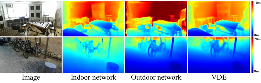
Figure 1: Versatile depth estimation: The indoor network, trained with indoor images only, performs poorly on an outdoor image. Similarly, the outdoor network is less effective for an indoor image. In contrast, the proposed VDE can estimate depths for both indoor and outdoor images reliably in a ‘versatile’ manner.

In this work, we propose a versatile depth estimator (VDE) to predict depth maps for scenes captured by different cameras, as illustrated in Figure 1. To this end, we design a common relative depth estimator (CRDE) and multiple relative-to-metric converters (R2MCs). First, the CRDE, composed of a transformer encoder and a transformer decoder, extracts relative depth information, which is camera-invariant. It adopts frequency mixing modules (FMMs) to transfer high-frequency components in encoder features to the decoder so that the decoder can predict a detailed relative depth map reliably. Second, each R2MC is employed to convert the relative depth map to the metric one corresponding to a specific camera. By training multiple R2MC modules, the proposed VDE can provide depth maps for multiple cameras. The versatility of VDE is demonstrated by extensive experiments on diverse datasets collected with seven different cameras. Moreover, VDE provides excellent metric depth estimation performance on the NYUv2 dataset [44].

This paper has the following contributions:

• We propose a versatile algorithm, called VDE, for monocular depth estimation, by developing the CRDE and R2MC modules.

• VDE yields excellent performance in diverse scenarios using different cameras, with only 1.7M parameters for each R2MC.

• VDE provides state-of-the-art performance on NYUv2 in the conventional single-camera scenario, as well as performing efficiently and effectively in the versatile scenarios.

2 Related Work

2.1 Monocular depth estimation

In monocular depth estimation, we infer the absolute distance of each scene point in a single image from the camera. Early monocular depth estimation focused on finding rough 3D layouts of scenes based on prior assumptions, such as superpixels [42], block world [17], or line segments and vanishing points [18]. Such assumptions, however, may be invalid, so unreliable depths may be obtained especially for small objects or regions with ambiguous colors.

CNNs have been adopted for monocular depth estimation successfully. Various attempts have been made to find effective network architecture [13, 27, 52, 20, 7] or loss functions [12, 6, 27, 21, 31]. Also, transformer [47] was recently applied to vision tasks [11], and its variants have been developed for monocular depth estimation [39, 56]. Besides, exploiting inherent information in 3D geometry, including virtual normal [55], depth attention volume [22], and depth distribution [3], has been tried to improve monocular depth estimation. Also, the depth estimation problem has been reformulated as ordinal regression [15], frequency domain analysis [29], and planar coefficient estimation [37].

2.2 Relative depth estimation

Relative depth estimation aims to learn the depth ranks of pixels in an image [58, 6, 51]. Since its objective is to determine not the absolute distances but the depth order of pixels, heterogeneous data — e.g. disparities from stereoscopic images [48, 50, 51], video frames [40], structure-from-motion (SfM) [34, 33], and human-annotated ordinal labels [6] — can be used jointly to train relative depth estimators. Moreover, relative depths are invariant to camera parameters, so images captured by different cameras can be used for training as well. The diversity of training data can lead to better depth estimation.

In relative depth estimation, the scale-invariant loss [13] and its variants [34, 33, 48, 40] have been used to cope with the scale ambiguity of depth labels. Recently, listwise ranking [35], instead of pairwise ranking, and depth normalization [23] have been considered.

2.3 Relative-to-metric depth conversion

Whereas relative depth information can be readily obtained from absolute depths in a metric depth map, the opposite conversion from relative depths to metric ones is not straightforward. There have been some attempts for this conversion. For instance, relative depths were fitted to metric depths directly using least-squares in [35, 40], and a relative depth estimator was fine-tuned to a metric depth estimator in [39]. Also, relative and metric depths were jointly learned through depth map decomposition in [23].

However, [35, 40] require a large depth-labeled dataset for fitting. Also, [39, 23] fine-tune a pre-trained network to estimate metric depth maps for a single camera only. Hence, they are not versatile, i.e., not applicable to images captured by different cameras. In contrast to these methods, the proposed VDE extracts relative depth information using a single CRDE for diverse cameras and then uses a simple R2MC module to convert the relative information to metric depths for a specific camera. Hence, VDE achieves versatile depth estimation efficiently: to support $N$ cameras, only $N$ R2MCs are required in addition to the CRDE. Moreover, by training the CRDE using diverse datasets, VDE yields comparable or even better performance than non-versatile techniques optimized for specific cameras.

2.4 Transformer and self-attention

Inspired by the success of the transformer architecture in natural language processing (NLP) [47, 10], transformers for vision tasks also have been studied extensively. In transformers, self-attention is performed to emphasize essential information and extract informative features. Many transformer-based neural networks [11, 36, 39, 14, 5] have been developed to provide even better performances than CNNs in vision tasks. Also, there have been researches for computing attention between different types of features [4, 8]. In this paper, we develop a transformer network for monocular depth estimation composed of an encoder and a decoder, as in U-Net [41]. In U-Net, skip connections can be used to transfer detailed information from the encoder to the decoder. Similarly, we propose FMMs to combine detailed information from the transformer encoder with the features of the transformer decoder effectively.

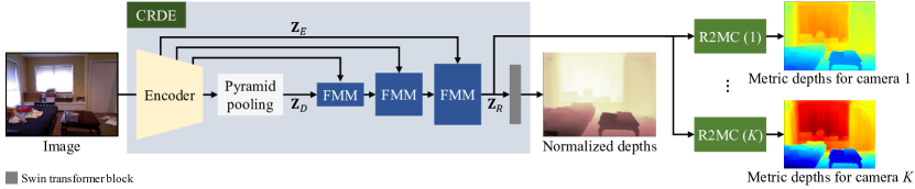
Figure 2: An overview of the proposed VDE: the CRDE extracts the relative depth feature ${\mathbf{Z}}_{R}$, which is processed to yield a normalized depth map. Also, ${\mathbf{Z}}_{R}$ is used to generate a metric depth map by the R2MC for the corresponding camera.

3 Proposed Algorithm

In Figure 2, the proposed VDE consists of a single CRDE for extracting relative depth information and multiple R2MCs for converting the information into metric depth maps for different cameras. In the CRDE, the Swin transformer [36] is adopted as the encoder, and three FMMs compose the decoder. Multi-scale encoder features are aggregated via pyramid pooling [57] and also transferred to the decoder via skip connections. The three FMMs are also based on the Swin transformer, but they mix the decoder feature ${\mathbf{Z}}_{D}$ with the encoder feature ${\mathbf{Z}}_{E}$ adaptively to yield the relative depth feature ${\mathbf{Z}}_{R}$. Then, the CRDE uses ${\mathbf{Z}}_{R}$ to produce a normalized depth map, while each R2MC module uses ${\mathbf{Z}}_{R}$ to yield a metric depth map. We can estimate metric depth maps for scenes captured by $K$ different cameras by training as many R2MCs.

3.1 Problem formulation

Let ${\mathbf{I}}$ be a color image and ${\mathbf{D}}$ be its depth map. In monocular depth estimation, an estimator $f$ is trained to minimize the loss

$$\sum_{({\mathbf{I}},{\mathbf{D}})\in{\cal T}}{\ell(f({\mathbf{I}}),{\mathbf{D}})}$$ (1)

where $\cal T$ is a training set of $({\mathbf{I}},{\mathbf{D}})$ pairs, and $\ell$ is a loss function between an estimated depth map $f({\mathbf{I}})$ and the ground-truth ${\mathbf{D}}$. Versatile monocular depth estimation is more challenging than ordinary one, for it should cope with images captured by diverse cameras with different parameters. Specifically, in versatile depth estimation, ${\cal T}$ in (1) is a union of multiple datasets, each of which is constructed with a different camera. To solve this problem, we decompose a depth map into camera-invariant and camera-specific components: relative depth information is camera-invariant, whereas depth scale information is camera-specific.

We adopt the normalized depth map as the camera-invariant component, as in [23]. Specifically, given a depth map ${\mathbf{D}}$, the normalized depth map ${\mathbf{N}}$ is obtained by

$$\textstyle{\mathbf{N}}=\frac{1}{\sigma}({\mathbf{D}}-\mu{\mathbf{U}})$$ (2)

where $\mu$ and $\sigma$ are the mean and standard deviation of depths in ${\mathbf{D}}$, and ${\mathbf{U}}$ is the unit matrix whose elements are all 1. Note that the CRDE estimates a normalized depth map in Figure 2. Thus, the CRDE, denoted by $g(\cdot)$, is trained to minimize the camera-invariant loss

$$L_{\textrm{CRDE}}=\sum_{({\mathbf{I}},{\mathbf{N}})\in\bigcup_{n=1}^{K}{\cal T}_{n}}{\ell(g({\mathbf{I}}),{\mathbf{N}})}$$ (3)

where ${\cal T}_{n}$ is the training set for camera $n$. Since the CRDE is common for all cameras, it is trained using all training sets $\bigcup_{n=1}^{K}{\cal T}_{n}$.

Given a normalized depth map ${\mathbf{N}}$, we can reconstruct the metric depth map ${\mathbf{M}}$ via (2) if $\mu$ and $\sigma$ are known. However, they are unknown in practice, and direct conversion is impossible. Hence, we first convert the relative depth feature ${\mathbf{Z}}_{R}$ into the metric depth feature for camera $n$ and then predict a metric depth map through an R2MC. Let $h_{n}$ denote the R2MC for camera $n$. It is trained to minimize the loss

$$L_{\textrm{R2MC}}^{(n)}=\sum_{({\mathbf{I}},{\mathbf{M}})\in{\cal T}_{n}}{\ell\left(h_{n}({\mathbf{Z}}_{R}({\mathbf{I}})),{\mathbf{M}}\right)}$$ (4)

where ${\mathbf{Z}}_{R}({\mathbf{I}})$ denotes the relative depth feature extracted from an image ${\mathbf{I}}$.

Finally, the overall loss for VDE is given by

$$L_{\textrm{overall}}=L_{\textrm{CRDE}}+\sum_{n=1}^{K}L_{\textrm{R2MC}}^{(n)}$$ (5)

where the first term is camera-invariant, and the second term is camera-specific.

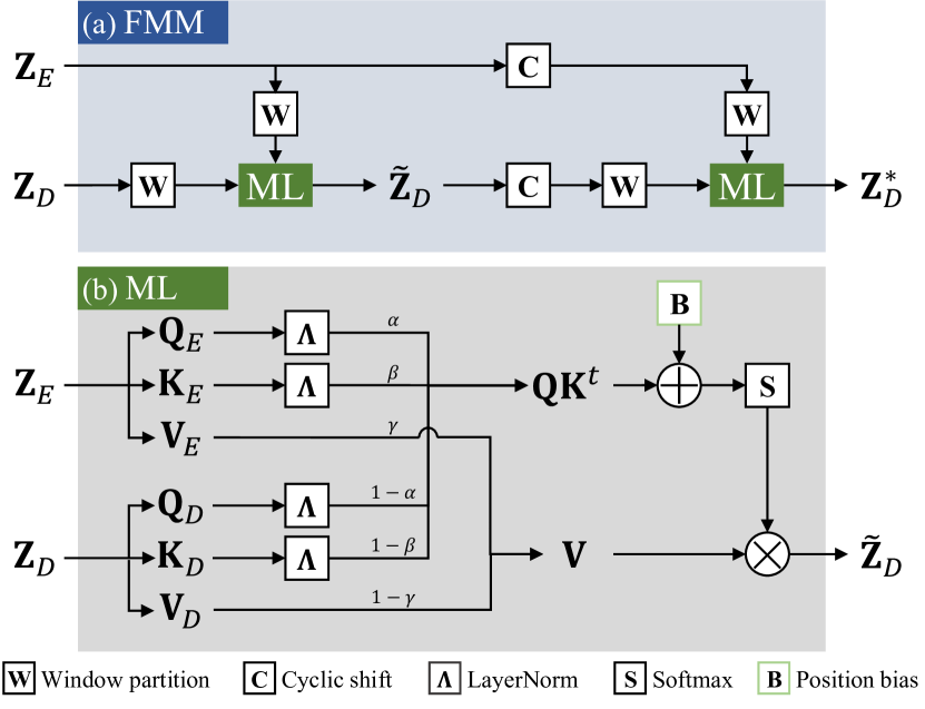
Figure 3: (a) The structure of an FMM and (b) the detailed structure of a mixing layer (ML).

3.2 CRDE

In monocular depth estimation, the encoder-decoder architecture in U-Net [41] is widely adopted for its efficacy. The encoder extracts a lower-resolution feature from an image, and then the decoder processes the feature to yield a depth map. At the decoder, interpolation or pixel shuffling is done to match an output resolution. However, the low-resolution feature may lose details, so skip connections are often used to pass details from the encoder to the decoder. In Figure 2, the CRDE also has the U-Net architecture, but it is composed of transformer blocks rather than convolution layers. In order to transfer high-frequency details, we employ three skip connections and compose the decoder with three FMMs.

In a typical depth map, planar regions — e.g. walls, floors, and ceilings — are dominant. Their depths change gradually and determine the overall 3D layout of a scene. Such depths are low-frequency components. In contrast, the depths of small objects or edge regions are mainly high-frequency components. Attempts have been made to reconstruct either low-frequency or high-frequency components reliably. For instance, in [20], the whole strip masking was proposed to detect low-frequency planar regions. On the other hand, to recover high-frequency details, gradient losses [21, 31] and contour information [38] have been exploited. In this paper, we develop FMMs to combine high-frequency details from the transformer encoder with reliable low-frequency information in the transformer decoder effectively.

Figure 3 shows the structure of an FMM, which combines a decoder feature ${\mathbf{Z}}_{D}\in\mathbb{R}^{C_{D}\times\frac{H}{2}\times\frac{W}{2}}$ with an encoder feature ${\mathbf{Z}}_{E}\in\mathbb{R}^{C_{E}\times H\times W}$. Note that the spatial resolution of ${\mathbf{Z}}_{D}$ is half of that of ${\mathbf{Z}}_{E}$. Hence, ${\mathbf{Z}}_{D}$ contains relatively low-frequency components. The FMM mixes ${\mathbf{Z}}_{D}$ with high-frequency details in ${\mathbf{Z}}_{E}$ to yield a refined, high-resolution feature ${\mathbf{Z}}^{*}_{D}\in\mathbb{R}^{C^{*}_{D}\times H\times W}$, given by

$$\begin{array}[]{l}{\mathbf{Z}}^{*}_{D}=\textrm{FMM}({\mathbf{Z}}_{E},{\mathbf{Z}}_{D}),\\ \end{array}$$ (6)

through an attention mechanism. An FMM is based on the Swin transformer block, so it contains two mixing layers in Figure 3(a). The first mixing layer combines ${\mathbf{Z}}_{E}$ and ${\mathbf{Z}}_{D}$ to yield $\widetilde{{\mathbf{Z}}}_{D}$, and then, after the cyclic shift [36], the second mixing layer processes ${\mathbf{Z}}_{E}$ and $\widetilde{{\mathbf{Z}}}_{D}$ to generate ${\mathbf{Z}}^{*}_{D}$.

Self-attention: Let us briefly summarize the self-attention mechanism [47, 11] in column vector notations, which are necessary to describe FMMs clearly. In a transformer block, an input feature map ${\mathbf{Z}}$ is spatially partitioned into $N$ tokens and expressed as

$${\mathbf{Z}}=\begin{bmatrix}z_{1}^{t}\\ \vdots\\ z_{N}^{t}\end{bmatrix}\in\mathbb{R}^{N\times C}$$ (7)

where each token $z_{n}$, $1\leq n\leq N$, is a $C$-dimensional column vector. Then, ${\mathbf{Z}}$ is transformed into the query, key, and value matrices by

$${\mathbf{Q}} =[q_{1},\cdots,q_{N}]^{t}={\mathbf{Z}}{\mathbf{U}}^{t}_{Q}$$ (8)

$${\mathbf{K}} =[k_{1},\cdots,k_{N}]^{t}={\mathbf{Z}}{\mathbf{U}}^{t}_{K}$$ (9)

$${\mathbf{V}} =[v_{1},\cdots,v_{N}]^{t}={\mathbf{Z}}{\mathbf{U}}^{t}_{V}$$ (10)

where ${\mathbf{U}}_{Q},{\mathbf{U}}_{K},{\mathbf{U}}_{V}\in\mathbb{R}^{P\times C}$ are projection matrices. By matching queries with keys, the attention matrix ${\mathbf{A}}$ is determined as

$${\mathbf{A}}=\textrm{softmax}\left(\frac{{\mathbf{Q}}{\mathbf{K}}^{t}}{\sqrt{N}}+\mathbf{B}\right)$$ (11)

where $\mathbf{B}$ is a position bias [36]. Finally, the self-attended output is given by

$${\mathbf{Z}}^{*}={\mathbf{A}}{\mathbf{V}}.$$ (12)

FMM: The encoder feature ${\mathbf{Z}}_{E}$ and the decoder feature ${\mathbf{Z}}_{D}$ are input to a mixing layer in FMM, as shown in Figure 3(b). They are reshaped into matrices of $N$ tokens, respectively;

$${\mathbf{Z}}_{E}=\begin{bmatrix}z_{E_{1}}^{t}\\ \vdots\\ z_{E_{N}}^{t}\end{bmatrix}\in\mathbb{R}^{N\times C_{E}},\,\,{\mathbf{Z}}_{D}=\begin{bmatrix}z_{D_{1}}^{t}\\ \vdots\\ z_{D_{N}}^{t}\end{bmatrix}\in\mathbb{R}^{N\times C_{D}^{\prime}}.$$ (13)

Note that two kinds of query matrices can be considered,

$${\mathbf{Q}}_{E} ={\mathbf{Z}}_{E}{\mathbf{U}}_{Q_{E}}^{t}$$ (14)

$${\mathbf{Q}}_{D} ={\mathbf{Z}}_{D}{\mathbf{U}}_{Q_{D}}^{t}$$ (15)

where ${\mathbf{U}}_{Q_{E}}\in\mathbb{R}^{P\times C_{E}}$ and ${\mathbf{U}}_{Q_{D}}\in\mathbb{R}^{P\times C_{D}^{\prime}}$. Similarly, we have two key matrices ${\mathbf{K}}_{E}$ and ${\mathbf{K}}_{D}$ and two value matrices ${\mathbf{V}}_{E}$ and ${\mathbf{V}}_{D}$. There are many possibilities for combining these query, value, and key matrices to yield the attended output ${\mathbf{Z}}^{*}$ in (12). For example, in [56], Yuan et al. obtained queries and keys from the encoder feature but values from the decoder feature. In other words, they set ${\mathbf{Q}}={\mathbf{Q}}_{E}$ and ${\mathbf{K}}={\mathbf{K}}_{E}$ in (11) and ${\mathbf{V}}={\mathbf{V}}_{D}$ in (12) to yield ${\mathbf{Z}}^{*}$.

Instead of the manual choice of query, key, and value matrices, we attempt to learn an optimal way to mix low-frequency base information in ${\mathbf{Z}}_{D}$ with high-frequency details in ${\mathbf{Z}}_{E}$. More specifically, as shown in Figure 3(b), we determine the query and key matrices by

$${\mathbf{Q}} =\alpha\cdot\Lambda({\mathbf{Q}}_{E})+(1-\alpha)\cdot\Lambda({\mathbf{Q}}_{D})$$ (16)

$${\mathbf{K}} =\beta\cdot\Lambda({\mathbf{K}}_{E})+(1-\beta)\cdot\Lambda({\mathbf{K}}_{D})$$ (17)

where $\alpha$ and $\beta$ are learnable mixing coefficients, and $\Lambda(\cdot)$ denotes the layer normalization [2]. Note that elements in ${\mathbf{Z}}_{E}$ may be in a different scale from those in ${\mathbf{Z}}_{D}$ does. For example, if ${\mathbf{Z}}_{D}$ consists of much larger elements than ${\mathbf{Z}}_{E}$ do, the softmax operation in (11) may be dominated by ${\mathbf{Z}}_{D}$ regardless of the relative importance of ${\mathbf{Z}}_{E}$ and ${\mathbf{Z}}_{D}$. To alleviate this scale issue, we adopt the layer normalization in (16) and (17). Also, note that ${\mathbf{Q}}{\mathbf{K}}^{t}$ in (11) is composed of four terms: ${\mathbf{Q}}_{E}{\mathbf{K}}_{E}^{t}$, ${\mathbf{Q}}_{E}{\mathbf{K}}_{D}^{t}$, ${\mathbf{Q}}_{D}{\mathbf{K}}_{E}^{t}$, and ${\mathbf{Q}}_{D}{\mathbf{K}}_{D}^{t}$. Because of ${\mathbf{Q}}_{E}{\mathbf{K}}_{D}^{t}$ and ${\mathbf{Q}}_{D}{\mathbf{K}}_{E}^{t}$, the cross-attention between the encoder feature and the decoder feature is performed. On the other hand, ${\mathbf{Q}}_{E}{\mathbf{K}}_{E}^{t}$ and ${\mathbf{Q}}_{D}{\mathbf{K}}_{D}^{t}$ are self-attention terms.

We also mix the encoder and decoder features to obtain the value matrix given by

$${\mathbf{V}}=\gamma\cdot{\mathbf{V}}_{E}+(1-\gamma)\cdot{\mathbf{V}}_{D}$$ (18)

where $\gamma$ is another learnable coefficient. It was observed that normalization is not necessary for ${\mathbf{V}}_{E}$ and ${\mathbf{V}}_{D}$.

By plugging (16), (17), (18) into (11) and (12), we obtain the refined decoder feature: $\widetilde{{\mathbf{Z}}}_{D}$ in the first mixing layer or ${\mathbf{Z}}_{D}^{*}$ in the second mixing layer. The output ${\mathbf{Z}}_{D}^{*}$ of an FMM is used as input to the next FMM. As shown in Figure 2, the output of the last FMM becomes the relative depth feature ${\mathbf{Z}}_{R}$, which is used to estimate a normalized depth map and also converted to a metric depth map by each R2MC module.

Figure 4: (a) The structure of an R2MC and (b) the detailed structure of a conversion layer (CL).

3.3 R2MC

For VDE to support $K$ cameras, we should implement and train $K$ R2MCs. In an R2MC for a specific camera, we first convert the relative depth feature ${\mathbf{Z}}_{R}$ from the CRDE into the metric depth feature ${\mathbf{Z}}_{M}$ optimized for that camera.

Similar to an FMM, an R2MC contains two conversion layers, as shown in Figure 4(a). The first conversion layer takes the relative depth feature ${\mathbf{Z}}_{R}$ and a learnable matrix ${\mathbf{L}}$ as input to generate the output

$$\widetilde{{\mathbf{L}}}=\textrm{softmax}\left(\frac{{\mathbf{Q}}_{R}{\mathbf{K}}_{R}^{t}}{\sqrt{N}}+{\mathbf{B}}\right){\mathbf{L}}$$ (19)

where ${\mathbf{Q}}_{R}$ and ${\mathbf{K}}_{R}$ are the query and key matrices obtained from ${\mathbf{Z}}_{R}$ through the self-attention in Figure 4(b). However, instead of the value matrix ${\mathbf{V}}_{R}$, a learnable matrix ${\mathbf{L}}$ is used in (19). Next, the second conversion layer takes ${\mathbf{Z}}_{R}$ and $\widetilde{{\mathbf{L}}}$ to provide the metric depth feature ${\mathbf{Z}}_{M}$. Finally, an ordinary Swin transformer block processes ${\mathbf{Z}}_{M}$ to yield a metric depth map ${\mathbf{M}}$.

By adopting a learnable matrix ${\mathbf{L}}$ in (19), each R2MC learns how to convert the relative depth feature ${\mathbf{Z}}_{R}$ into the camera-specific metric depth feature ${\mathbf{Z}}_{M}$. Thus, ${\mathbf{L}}$ plays the role of a camera-specific mapping function from the relative depth space to the metric one. Each R2MC requires only 1.7M parameters, so the proposed VDE can be implemented at the cost of only a moderate increase in complexity.

3.4 Loss function

We use the scale-invariant logarithmic loss function $\ell$ for both $L_{\textrm{CRDE}}$ in (3) and $L_{\textrm{R2MC}}$ in (4). Let $d_{i}$ and $\hat{d}_{i}$ denote the $i$th depths in the ground-truth depth map ${\mathbf{D}}$ and a predicted depth map $\hat{{\mathbf{D}}}$, respectively. Then, the loss function is defined as

$$\ell(\hat{{\mathbf{D}}},{\mathbf{D}})=\alpha\sqrt{\frac{1}{|{\mathbf{D}}|}\sum_{i}{{e_{i}}^{2}}-\frac{\lambda}{|{\mathbf{D}}|^{2}}(\sum_{i}{e_{i}})^{2}}$$ (20)

where $e_{i}=\log\hat{d}_{i}-\log d_{i}$, and $|{\mathbf{D}}|$ denotes the number of valid pixels in ${\mathbf{D}}$. As in [3, 56], we set $\alpha=10$ and $\lambda=0.85$.

Table 1: Scene types and cameras for the five datasets.

NYUv2	DIML	DIODE	ScanNet	SUN RGB-D
Indoor	Indoor, Outdoor	Indoor, Outdoor	Indoor	Indoor
Kinect v1	Kinect v2,	Laser scanner	Structure sensor	Kinect v1, Kinect v2
	ZED stereo			RealSense, Xtion

4 Experimental Results

4.1 Datasets

To assess the versatile depth estimation performance and reliability of the proposed VDE in diverse scenarios, we use five datasets: NYUv2 [44], DIML [25], DIODE [46], ScanNet [9], and SUN RGB-D [45]. They are divided into 10 sub-datasets according to the scene types and the cameras. Specifically, DIML and DIODE contain indoor and outdoor scenes, so they are, respectively, partitioned into two sub-datasets according to the scene types. Also, SUN RGB-D is divided into four sub-datasets depending on the cameras for the data acquisition. Table 1 summarizes the five datasets. More detailed information on the datasets is provided in the appendix (Section B).

4.2 Evaluation metrics

Metric depth assessment: We adopt the top four metrics in Table 2 and follow the protocol in [28, 3, 23, 56], in which only the regions with valid ground-truth depths are taken into account in the evaluation.

Relative depth assessment: We use the bottom two metrics in Table 2. First, ‘Relative $\delta_{1}$’ measures $\delta_{1}$ between a calibrated relative depth map $\tilde{{\mathbf{R}}}$ and the ground-truth metric depth map ${\mathbf{D}}$. As in [40, 39], for a predicted relative depth map $\hat{{\mathbf{R}}}$, the calibrated depth map is given by $\tilde{{\mathbf{R}}}=m\hat{{\mathbf{R}}}+b\mathbf{1}$, where $\mathbf{1}$ is the depth map consisting of all $1$’s. For each image, the scaling parameter $m$ and the shift parameter $b$ are adjusted to minimize the least square error between $\tilde{{\mathbf{R}}}$ and ${\mathbf{D}}$. Second, Kendall’s $\tau$ [24] quantifies the confidence of the depth order among pixels by considering the number of concordant and discordant pixel pairs in $\hat{{\mathbf{D}}}$ and ${\mathbf{D}}$. A higher Kendall’s $\tau$ indicates a better result.

Table 2: Evaluation metrics for depth maps. The top four are for metric depths, while the bottom two are for relative depths. Here, $|{\mathbf{D}}|$ denotes the number of valid pixels in a depth map ${\mathbf{D}}$, $d_{i}$ is the $i$th valid depth in ${\mathbf{D}}$, and $\hat{d}_{i}$ is an estimate of $d_{i}$. Also, $\operatorname{sgn}(\cdot)$ is the sign function returning 1 for a positive value and 0 otherwise.

RMSE	$\frac{1}{|{\mathbf{D}}|}\big{(}\sum_{i}(\hat{d}_{i}-d_{i})^{2}\big{)}^{0.5}$
REL	$\frac{1}{|{\mathbf{D}}|}\sum_{i}|\hat{d}_{i}-d_{i}|/d_{i}$
$\log$$10$	$\frac{1}{|{\mathbf{D}}|}\sum_{i}|\log_{10}(\hat{d}_{i})-\log_{10}(d_{i})|$
$\delta_{k}$, $k=1,2,3$	% of $d_{i}$ that satisfies $\max\!\left\{\frac{\hat{d}_{i}}{d_{i}},\frac{d_{i}}{\hat{d}_{i}}\right\}<1.25^{k}$
Relative $\delta_{1}$	$\delta_{1}$ between $\tilde{{\mathbf{R}}}=m\hat{{\mathbf{R}}}+b\mathbf{1}$ and ${\mathbf{D}}$
Kendall’s $\tau$	$\frac{1}{\binom{|{\mathbf{D}}|}{2}}\sum_{i}\sum_{j}\mathrm{sgn}\big{(}(\hat{d}_{i}-\hat{d}_{j})(d_{i}-d_{j})\big{)}$

4.3 Implementation details

Network architecture: In Figure 2, as the encoder of VDE, we adopt Swin-Base [36], which takes an RGB image of spatial resolution $H\times W$ to generate multi-scale features. Then, the pyramid pooling [57] combines those features to produce the decoder feature ${\mathbf{Z}}_{D}$ of resolution $\frac{H}{32}\times\frac{W}{32}$. The decoder consists of three FMMs, each of which doubles the spatial resolution. The output of the last FMM is the relative depth feature ${\mathbf{Z}}_{R}$, which is fed to a Swin transformer block to yield a normalized depth map. Also, using ${\mathbf{Z}}_{R}$, each R2MC estimates the metric depth map captured by the corresponding camera. The resolution of the relative depth map and the metric depth maps is $\frac{H}{4}\times\frac{W}{4}$, so we interpolate them bilinearly to the original $H\times W$ resolution.

Training: VDE is trained in two steps. First, we train only CRDE to estimate normalized depth maps, after initializing the encoder with a pre-trained Swin-Base on ImageNet [36]. Second, we train the complete network to produce metric depth maps for different cameras. In both steps, the Adam optimizer [26] is used with a batch size of 4 and a weight decay of $10^{-2}$. The initial learning rate is set to $2\times 10^{-5}$, and it decreases linearly to $1\times 10^{-6}$. Normalized depth losses are computed by (3), while, in the second step, metric depth losses are evaluated separately for different cameras via (4). The elements of the learnable matrix ${\mathbf{L}}$ in each R2MC are initialized to $2\times 10^{-2}$, and $\alpha,\beta$, and $\gamma$ in each FMM are initialized to 0.5.

Figure 5: Four network structures for versatile depth estimation.

4.4 Versatile depth estimation

We compare versatile depth estimation results of the proposed VDE and three alternative settings. Figure 5 illustrates the network structures of these settings. ‘Single network’ optimizes one CRDE using all 10 sub-datasets, while ‘Separate networks’ optimize 10 CRDEs separately for the 10 sub-datasets. In ‘Multiple decoders,’ a shared encoder is trained jointly with 10 decoders, each of which consists of three FMMs and a Swin transformer block. Finally, VDE is trained using a shared CRDE and 10 separate R2MCs.

Since each sub-dataset has a different size, data imbalance can be incurred. Hence, we sample 1,000 images from each sub-dataset, except for the RealSense sub-dataset of SUN RGB-D, for which we use all 587 images available. VDE is trained for 64 epochs, while ‘Single network,’ ‘Separate networks,’ and ‘Multiple decoders’ are trained for 64, 640, and 64 epochs, respectively. Therefore, the four settings are trained for similar numbers of iterations.

Figure 6: Comparison of $\delta_{1}$ and Kendall’s $\tau$ results of the four settings on the 10 sub-datasets.

Table 3: Comparison of versatile depth estimation results of ‘Separate networks,’ ‘Multiple decoders,’ and VDE. For each setting, the required number of parameters is specified. Lower RMSE and REL indicate better results, whereas higher $\delta_{1}$ and $\tau$ are better. In each test, the best result is boldfaced.

Setting	Dataset	RMSE$(\downarrow)$	REL$(\downarrow)$	$\delta_{1}(\uparrow)$	$\tau(\uparrow)$
Separate networks (149.8M ​​ $\times$ ​​ 10)	NYUv2	0.376	0.111	0.892	0.811
	DIML-Indoor	0.693	0.244	0.640	0.585
	DIML-Outdoor	1.240	0.142	0.812	0.828
	DIODE-Indoor	1.352	0.255	0.569	0.543
	DIODE-Outdoor	5.880	0.302	0.615	0.646
	ScanNet	0.347	0.169	0.774	0.691
	SUN (Kinect v1)	0.324	0.157	0.803	0.754
	SUN (Kinect v2)	0.257	0.099	0.912	0.829
	SUN (RealsSense)	0.245	0.104	0.893	0.782
	SUN (Xtion)	0.405	0.416	0.784	0.720
Multiple decoders (571.3M)	NYUv2	0.380	0.109	0.894	0.817
	DIML-Indoor	0.662	0.235	0.673	0.616
	DIML-Outdoor	1.356	0.148	0.800	0.838
	DIODE-Indoor	1.180	0.217	0.638	0.644
	DIODE-Outdoor	6.973	0.351	0.485	0.633
	ScanNet	0.340	0.185	0.753	0.739
	SUN (Kinect v1)	0.349	0.184	0.753	0.770
	SUN (Kinect v2)	0.330	0.168	0.797	0.827
	SUN (RealsSense)	0.223	0.110	0.906	0.799
	SUN (Xtion)	0.417	0.467	0.748	0.745
VDE (167.3M)	NYUv2	0.335	0.093	0.925	0.848
	DIML-Indoor	0.653	0.228	0.678	0.635
	DIML-Outdoor	1.245	0.146	0.846	0.853
	DIODE-Indoor	1.175	0.222	0.645	0.693
	DIODE-Outdoor	6.141	0.334	0.566	0.642
	ScanNet	0.295	0.139	0.830	0.778
	SUN (Kinect v1)	0.287	0.125	0.863	0.804
	SUN (Kinect v2)	0.231	0.088	0.939	0.857
	SUN (RealsSense)	0.215	0.098	0.925	0.832
	SUN (Xtion)	0.363	0.411	0.838	0.784

Figure 6 compares the four settings in terms of $\delta_{1}$ and Kendall’s $\tau$. Also, Table 3 provides detailed comparisons of ‘Separate networks,’ ‘Multiple decoders,’ and the proposed VDE on the 10 sub-datasets. The worst-performing ‘Single network’ is excluded from Table 3. The following observations can be made from Figure 6 and Table 3:

• By using only 167.3M parameters, VDE generally outperforms ‘Separate networks’ and ‘Multiple decoders’ using 1,498M and 571.3M parameters, respectively. It is worth pointing out that VDE requires 1.7M parameters only to add an R2MC for a new camera.

• Even when compared with ‘Separate networks’ optimized for each camera, VDE performs better in most tests. Note that VDE is more effective for indoor images than for outdoor ones (DIML-Outdoor and DIODE-Outdoor) because the ratio of indoor to outdoor training images is about 8 to 2 in this experiment. However, even on the outdoor images, VDE yields comparable results to ‘Separate networks.’

• On the other hand, on the indoor images, VDE meaningfully outperforms ‘Separate networks.’ For example, in Kendall’s $\tau$ on DIODE-Indoor, VDE surpasses ‘Separate networks’ by a large margin of 0.150.

• Furthermore, VDE performs better than ‘Multiple decoders’ because it trains more parts of the network jointly using heterogenous data with the common goal of estimating normalized depth maps accurately.

• Overall, VDE yields reliable depth estimation results on both indoor and outdoor images. In general, outdoor images have different depth scales from indoor ones. This is a reason why ‘Single network’ performs poorly in Figure 6. In contrast, VDE overcomes the scale differences between indoor and outdoor scenes by adopting an R2MC for each camera. This is beneficial since a practical algorithm should be capable of handling diverse scenes and cameras.

Figure 7 shows examples of estimated depth maps. We see that VDE yields more reliable depth maps for diverse images than the alternative settings do.

More experimental results, including cross-dataset evaluation and tests on heterogeneous datasets of different sizes, are in the appendix (Section C).

Figure 7: Examples of versatile depth estimation results.

4.5 Ordinary depth estimation

Although the primary focus of VDE is versatile depth estimation, it achieves state-of-the-art performance in ordinary depth estimation as well. Table 4 assesses the metric depth performance of VDE on the NYUv2 dataset. Earlier algorithms [13, 49, 27, 15, 21, 7, 38, 55, 31] perform evaluation by filling in missing ground-truth depths using a colorization scheme [32]. We distinguish those from recent ones [28, 3, 53, 39, 23, 37, 56] that use valid depths only.

For ordinary depth estimation, one VDE model with a single R2MC is trained only on the NYUv2 dataset for 30 epochs. We use Swin-Large [36] as the encoder for a fair comparison with existing state-of-the-art methods [56, 1]. The proposed VDE surpasses all conventional methods in four out of six metrics. Furthermore, VDE^∗ using extra training data from Table 1 for the CRDE provides an additional performance boost. This indicates that training a more reliable CRDE using different cameras can further improve the depth estimation performance for an individual camera. Note that the same observation can be made from Table 3: VDE performs better than ‘Separate networks.’ Figure 8 compares qualitative results of VDE^∗ with those of conventional algorithms [15, 3, 56], confirming that VDE^∗ estimates depths more accurately with fewer artifacts. Metric depth estimation results on the KITTI dataset [16] are in the appendix (Section D).

Table 4: Comparison of depth estimation results on NYUv2. For each metric, the best result is boldfaced, and the second best is underscored. $*$ means that additional data is used for training.

Method	RMSE$(\downarrow)$	REL$(\downarrow)$	$\log$$10$$(\downarrow)$	$\delta_{1}(\uparrow)$	$\delta_{2}(\uparrow)$	$\delta_{3}(\uparrow)$
Eigen et al. [13]	0.641	0.158	-	0.769	0.950	0.988
Wang et al. [49]∗	0.745	0.220	0.094	0.605	0.890	0.970
Laina et al. [27]	0.573	0.127	0.055	0.811	0.953	0.988
Hao et al. [19]	0.555	0.127	0.053	0.841	0.966	0.991
Fu et al. [15]	0.509	0.115	0.051	0.828	0.965	0.992
Hu et al. [21]	0.530	0.115	0.050	0.866	0.975	0.993
Chen et al. [7]	0.514	0.111	0.048	0.878	0.977	0.994
Ramam. et al. [38]∗	0.495	0.139	0.047	0.888	0.979	0.995
Yin et al. [55]	0.416	0.108	0.048	0.875	0.976	0.994
Hyunh et al. [22]	0.412	0.108	-	0.882	0.980	0.996
Lee and Kim [31]	0.430	0.119	0.050	0.870	0.974	0.993
Lee et al. [28]	0.392	0.110	0.047	0.885	0.978	0.994
Bhat et al. [3]	0.364	0.103	0.044	0.903	0.984	0.997
Yang et al. [53]	0.365	0.106	0.045	0.900	0.983	0.996
Ranftl et al. [39]∗	0.357	0.110	0.045	0.904	0.988	0.998
Jun et al. [23]∗	0.355	0.098	0.042	0.913	0.987	0.998
Patil et al. [37]	0.356	0.104	0.043	0.898	0.981	0.996
Yuan et al. [56]	0.334	0.095	0.041	0.922	0.992	0.998
Agar. and Arora [1]	0.322	0.090	0.039	0.929	0.991	0.998
VDE	0.315	0.088	0.038	0.934	0.991	0.998
VDE∗	0.290	0.080	0.035	0.949	0.993	0.998

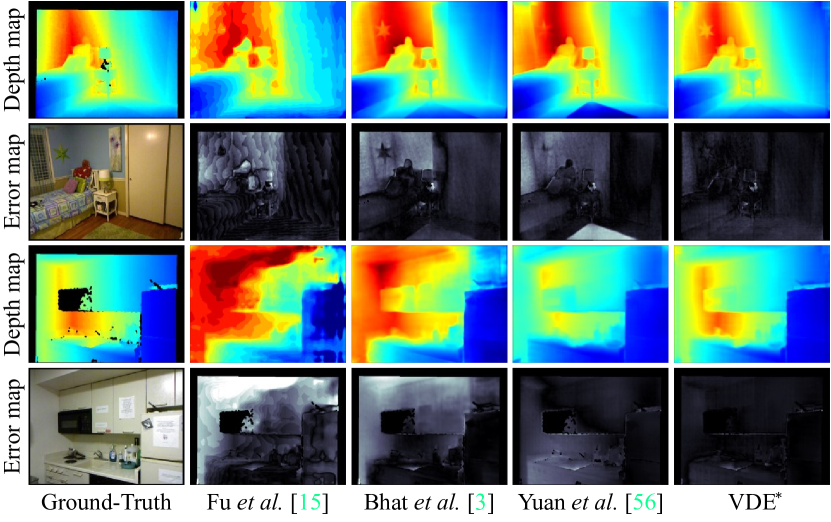
Figure 8: Qualitative results on NYUv2. For each depth map, the error map is provided with brighter pixels indicating larger errors.

4.6 Analysis

To evaluate the generalization performance on unseen data, we compare the proposed CRDE with existing relative depth estimators MiDaS [40] and DPT-Large [39], which do not use NYUv2 for their training. Table 5 compares relative $\delta_{1}$ and Kendall’s $\tau$ results on NYUv2. In this test, we train the CRDE on the datasets in Table 1, excluding NYUv2 and SUN (Kinect v1) captured with Kinect v1. The CRDE performs well on the unseen images as well, for it is trained to estimate normalized (i.e. relative) depths reliably for diverse datasets. Hence, it surpasses the existing estimators.

Table 5: Comparison of relative $\delta_{1}$ and Kendall’s $\tau$ results on NYUv2.

	# Params	Relative $\delta_{1}(\uparrow)$	Kendall’s $\tau(\uparrow)$
MiDaS [40]	105.4M	0.894	0.746
DPT [39]	344.1M	0.905	0.764
CRDE	149.8M	0.924	0.843

Table 6: Ablation studies of VDE on NYUv2.

Settings	RMSE$(\downarrow)$	REL$(\downarrow)$	$\delta_{1}(\uparrow)$	$\tau(\uparrow)$
Baseline	0.335	0.094	0.922	0.844
+ FMM	0.330	0.092	0.926	0.848
+ R2MC	0.329	0.093	0.924	0.854
+ FMM + R2MC	0.325	0.091	0.926	0.858

Table 7: Impacts of hyperparameters in FMMs. NYUv2 is used in this test.

$\alpha$	$\beta$	$\gamma$	RMSE$(\downarrow)$	REL$(\downarrow)$	$\delta_{1}(\uparrow)$	$\tau(\uparrow)$
0	0	0	0.335	0.094	0.922	0.844
1	1	0	0.331	0.093	0.923	0.847
0	0	1	0.341	0.094	0.920	0.841
0.5	0.5	0.5	0.332	0.093	0.924	0.849
Learnable			0.330	0.092	0.926	0.848

In Table 6, we test ablated methods of VDE on NYUv2. ‘Baseline’ is a basic encoder-decoder network using ordinary Swin transformer blocks instead of FMMs. It estimates metric depths directly, instead of normalized depths, with no R2MC. We see that both FMMs and R2MC lead to performance improvements.

Table 7 compares the results when learnable mixing coefficients $\alpha,\beta,\gamma$ in FMMs are fixed as follows:

1. The decoder feature is not mixed with the encoder feature ($\alpha=0,\beta=0,\gamma=0$).

2. Queries and keys are obtained from the encoder feature, while values from the decoder feature, as in [56] ($\alpha=1,\beta=1,\gamma=0$).

3. The opposite to case 2 ($\alpha=0,\beta=0,\gamma=1$).

4. The encoder and decoder features are equally mixed ($\alpha=0.5,\beta=0.5,\gamma=0.5$).

Without testing all combinations, ‘Learnable’ yields the best results. More detailed analyses of FMMs and R2MCs are conducted in the appendix (Section F).

5 Conclusions

We proposed a novel VDE composed of a single CRDE and multiple R2MCs. First, the CRDE generates common relative depth features. Then, the R2MCs convert the relative features to camera-specific metric depth maps. It was shown that VDE is applicable to versatile depth estimation successfully, as well as providing state-of-the-art performance in the single-camera scenario. More specifically, VDE yields comparable or better performance than non-versatile techniques optimized for specific cameras, while requiring only a 1.12% parameter increase per camera.

Appendix A Network Architecture

Figure 9 shows the network structure of the proposed VDE. As the encoder, we adopt Swin-Base [36], which processes a $480\times 640$ RGB image to yield the multi-scale encoder feature ${\mathbf{Z}}_{E}$. Then, we compress ${\mathbf{Z}}_{E}$ via pyramid pooling [57] to generate the decoder feature ${\mathbf{Z}}_{D}$ of size $512\times 15\times 20$. Next, we process ${\mathbf{Z}}_{D}$ sequentially using three FMMs with pixel shuffling layers to yield the relative depth feature ${\mathbf{Z}}_{R}$ of size $64\times 120\times 160$. We then concatenate ${\mathbf{Z}}_{R}$ with ${\mathbf{E}}_{1}$ from the encoder to perform the normalized depth estimation. Also, we feed ${\mathbf{Z}}_{R}$ to $K$ R2MCs to generate metric depths for the corresponding cameras. The detailed structures of FMMs and R2MCs are in Figure 3 and Figure 4, respectively.

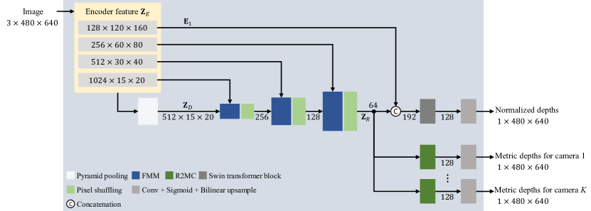
Figure 9: Network structure of the proposed VDE. The number of channels in each feature tensor is specified.

Appendix B Dataset Specifications

Table 8 summarizes the camera specifications and the training and test images for each dataset. For NYUv2, we adopt the training split in [3, 28, 56]. For ScanNet, we sample every 100th and 200th frames from the official training and test scans, respectively. For versatile depth estimation, we sample the training images in a dataset uniformly to construct each sub-dataset of 1,000 images, except for SUN (RealSense) for which we use all 587 images available. SUN RGB-D includes Kinect v1 and Kinect v2 images. However, these images have different characteristics from NYUv2 and DIML-Indoor ones because SUN RGB-D performs post-processing differently to improve the depth maps. We also conduct additional experiments using KITTI and HR-WSI. We adopt the Eigen split [12] of KITTI and the official split of HR-WSI.

Table 8: Dataset specifications

Dataset	Scene type	Camera	Field of view	Depth range	Training images	Test images
NYUv2 [44]	Indoor	Kinect v1	43°$\times$ 57°	0.4$\sim$4.0m	36,253	654
DIML [25]	Indoor	Kinect v2	60°$\times$ 70°	0.5$\sim$8.0m	1,609	504
	Outdoor	ZED stereo	60°$\times$ 90°	0.5$\sim$20m	1,505	500
DIODE [46]	Indoor	Laser scanner	305°$\times$ 360°	0.6$\sim$350m	8,574	325
	Outdoor				16,884	446
ScanNet [9]	Indoor	Structure sensor	45°$\times$ 58°	0.4$\sim$3.5m	25,536	1,084
SUN RGB-D [45]	Indoor	Kinect v1	43°$\times$ 57°	0.4$\sim$4.0m	1,073	930
		Kinect v2	60°$\times$ 70°	0.5$\sim$8.0m	1,924	1,860
		RealSense	43°$\times$ 70°	0.4$\sim$2.8m	587	572
		Xtion	45°$\times$ 58°	0.8$\sim$3.5m	1,701	1,688
KITTI [16]	Outdoor	HDL-64E	26.8°$\times$ 360°	2.5$\sim$80m	23,158	697
HR-WSI [51]	Indoor & Outdoor	Stereo image pairs			20,378	400

Appendix C Versatile Depth Estimation

C.1 Extended VDE test

Table 9 is an extended version of Table 3, including the results of ‘Single network.’ Also, for an easier comparison, we report the geometric mean scores over the 10 sub-datasets.

Table 9: Comparison of versatile depth estimation results. For each setting, the required number of parameters is specified. Lower RMSE and REL indicate better results, while higher $\delta_{1}$ and $\tau$ are better ones. In each test, the best result is boldfaced.

Setting	Dataset	RMSE$(\downarrow)$	REL$(\downarrow)$	$\delta_{1}(\uparrow)$	$\tau(\uparrow)$
Single network (149.8M)	NYUv2	0.413	0.121	0.862	0.813
	DIML-Indoor	0.916	0.333	0.478	0.573
	DIML-Outdoor	3.172	0.373	0.328	0.693
	DIODE-Indoor	2.607	0.462	0.123	0.479
	DIODE-Outdoor	15.647	0.797	0.005	0.574
	ScanNet	0.414	0.225	0.658	0.719
	SUN (Kinect v1)	0.402	0.227	0.672	0.764
	SUN (Kinect v2)	0.504	0.275	0.517	0.811
	SUN (RealsSense)	0.307	0.162	0.795	0.792
	SUN (Xtion)	0.513	0.551	0.611	0.731
	Mean	0.957	0.305	0.314	0.685
Separate networks (149.8M ​​ $\times$ ​​ 10)	NYUv2	0.376	0.111	0.892	0.811
	DIML-Indoor	0.693	0.244	0.640	0.585
	DIML-Outdoor	1.240	0.142	0.812	0.828
	DIODE-Indoor	1.352	0.255	0.569	0.543
	DIODE-Outdoor	5.880	0.302	0.615	0.646
	ScanNet	0.347	0.169	0.774	0.691
	SUN (Kinect v1)	0.324	0.157	0.803	0.754
	SUN (Kinect v2)	0.257	0.099	0.912	0.829
	SUN (RealsSense)	0.245	0.104	0.893	0.782
	SUN (Xtion)	0.405	0.416	0.784	0.720
	Mean	0.612	0.179	0.760	0.712
Multiple decoders (571.3M)	NYUv2	0.380	0.109	0.894	0.817
	DIML-Indoor	0.662	0.235	0.673	0.616
	DIML-Outdoor	1.356	0.148	0.800	0.838
	DIODE-Indoor	1.180	0.217	0.638	0.644
	DIODE-Outdoor	6.973	0.351	0.485	0.633
	ScanNet	0.340	0.185	0.753	0.739
	SUN (Kinect v1)	0.349	0.184	0.753	0.770
	SUN (Kinect v2)	0.330	0.168	0.797	0.827
	SUN (RealsSense)	0.223	0.110	0.906	0.799
	SUN (Xtion)	0.417	0.467	0.748	0.745
	Mean	0.632	0.196	0.734	0.738
VDE (167.3M)	NYUv2	0.335	0.093	0.925	0.848
	DIML-Indoor	0.653	0.228	0.678	0.635
	DIML-Outdoor	1.245	0.146	0.846	0.853
	DIODE-Indoor	1.175	0.222	0.645	0.693
	DIODE-Outdoor	6.141	0.334	0.566	0.642
	ScanNet	0.295	0.139	0.830	0.778
	SUN (Kinect v1)	0.287	0.125	0.863	0.804
	SUN (Kinect v2)	0.231	0.088	0.939	0.857
	SUN (RealsSense)	0.215	0.098	0.925	0.832
	SUN (Xtion)	0.363	0.411	0.838	0.784
	Mean	0.559	0.164	0.795	0.768

C.2 Cross-dataset evaluation

Note that each R2MC is optimized for a specific camera. In this test, we conduct cross-dataset evaluation, which assesses the relative depth estimation results of each R2MC on different datasets obtained with different cameras. We measure Kendall’s $\tau$ scores, since the metrics for metric depth estimation are inappropriate for this evaluation across different cameras.

First, Figure 10 compares depth maps obtained by the proposed R2MCs for NYUv2, DIML-Outdoor, and DIODE-Outdoor for the same input images. It can be observed that, for each input image, the three depth maps contain similar relative depth information even though their depth scales are different. In other words, each R2MC predicts relative depth orders reliably even for images captured with different cameras.

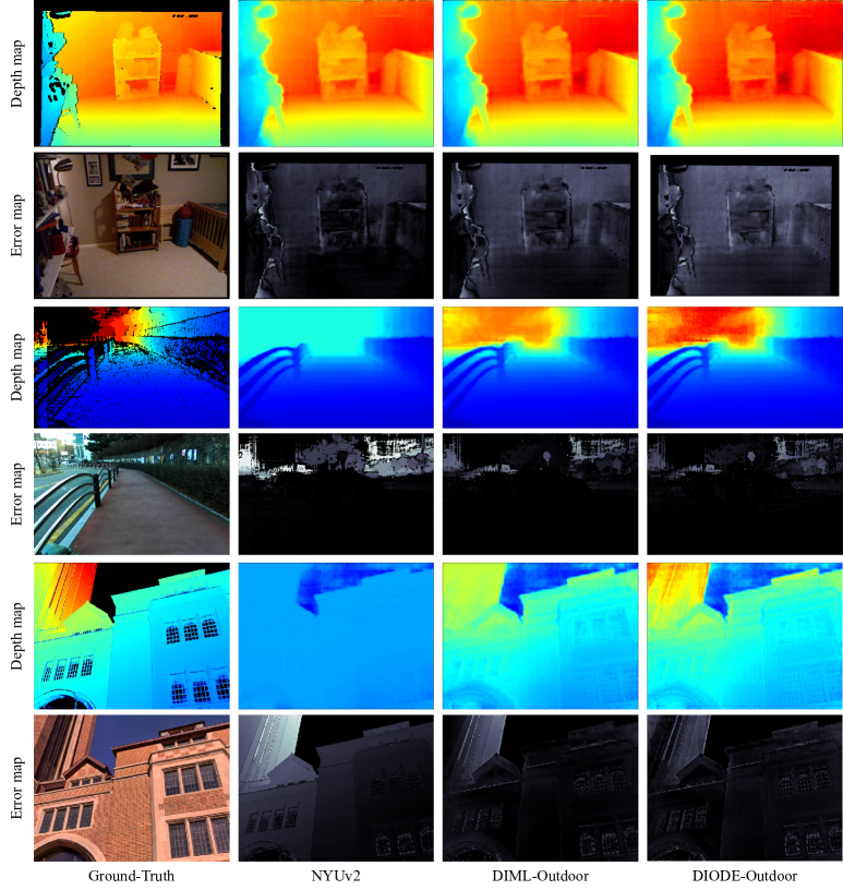
Figure 10: For each input image, three depth maps, obtained by the R2MCS for NYUv2, DIML-Outdoor, and DIODE-Outdoor, are provided with the corresponding error maps. From top to bottom, the input images are from the NYUv2, DIML-Outdoor, and DIODE-Outdoor test datasets.

Next, Figure 11 and Figure 12 compare Kendall’s $\tau$ scores in this cross-dataset evaluation. For example, the top left graph in Figure 11 compares the Kendall’s $\tau$ scores on the NYUv2 test images obtained by the 10 R2MCs for the 10 sub-datasets. Since only a single score is generated by ‘Single network,’ it is repeated for the 10 R2MCs. We see that ‘Separate networks’ are fitted to the corresponding sub-datasets and perform poorly on the other datasets in general, while ‘Multiple decoders’ and VDE provide consistent Kendall’s $\tau$ scores. However, VDE outperforms ‘Multiple decoders,’ indicating that sharing more portions of the network for the common goal of normalized depth estimation via CRDE improves the generalization performance. In the main paper, it is shown that VDE surpasses the other settings in metric depth evaluation as well, indicating that R2MC successfully transforms relative depth features into metric depths.

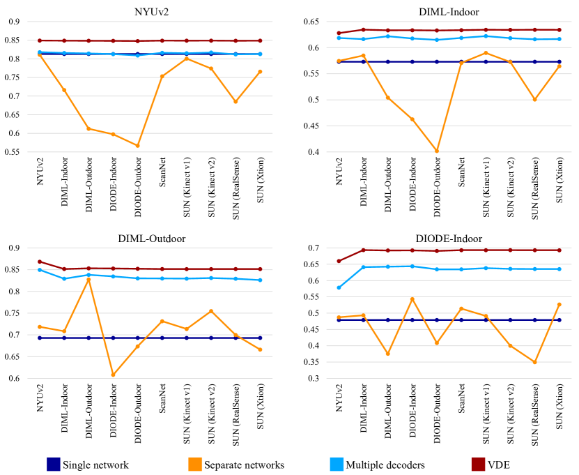
Figure 11: Comparison of Kendall’s $\tau$ scores in the cross-dataset evaluation.

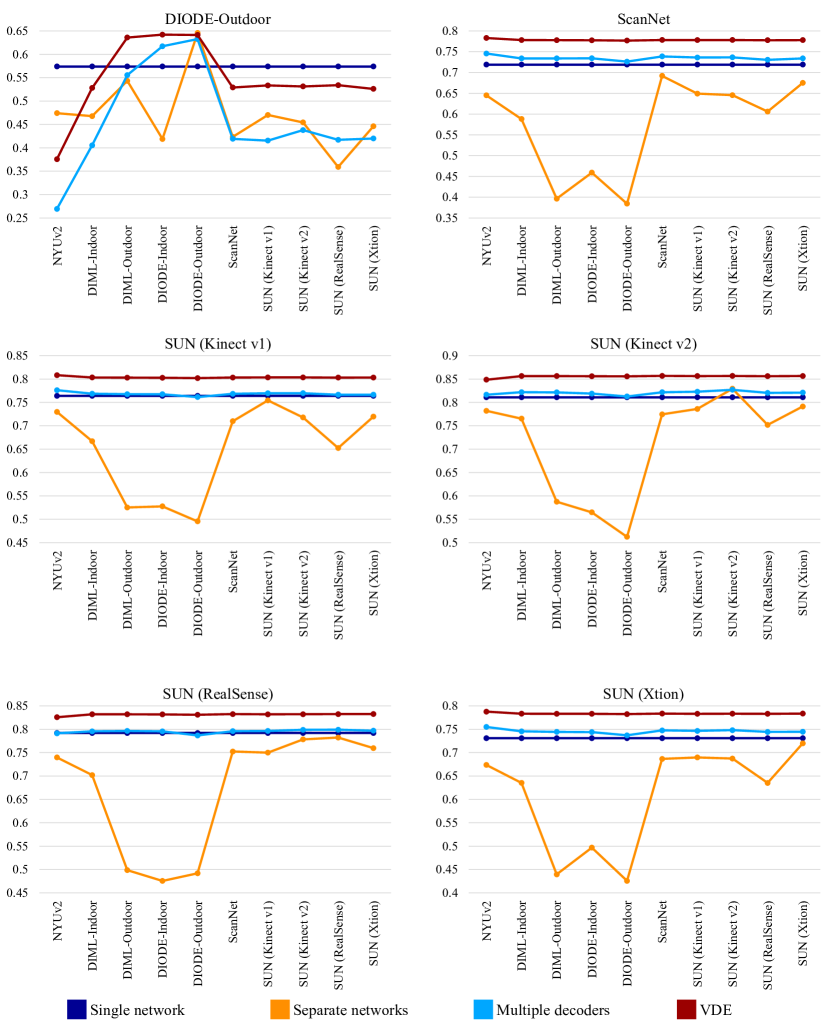
Figure 12: Comparison of Kendall’s $\tau$ scores in the cross-dataset evaluation.

C.3 VDE using multiple datasets of different sizes

In real-world applications of VDE, different datasets may have different sizes. We hence evaluate the performances of VDE using multiple datasets of various sizes in Table 10. In this experiment, we use the whole training datasets of NYUv2 and DIML, which are specified in Table 8. Since NYUv2 contains much more training images than DIML, each DIML image is used five times per epoch while each NYUv2 image is used only once per epoch during the training. Similarly to Table 3, the proposed VDE outperforms ‘Separate networks’ on indoor images. Especially, note that VDE surpasses ‘Separate networks’ even on NYUv2, for which ‘Separate network’ is optimized with a relatively large number of training images.

Table 10: Comparison of versatile depth estimation results using uneven sized datasets.

Setting	Dataset	# data	RMSE$(\downarrow)$	REL$(\downarrow)$	$\delta_{1}(\uparrow)$	$\tau(\uparrow)$
Separate networks (149.8M ​​ $\times$ ​​ 3)	NYUv2	36,253	0.330	0.092	0.926	0.848
	DIML-Indoor	1,609	0.683	0.246	0.650	0.589
	DIML-Outdoor	1,505	1.180	0.135	0.830	0.840
	Mean		0.643	0.145	0.793	0.749
VDE (155.1M)	NYUv2	36,253	0.322	0.091	0.928	0.859
	DIML-Indoor	1,609	0.667	0.239	0.662	0.629
	DIML-Outdoor	1,505	1.217	0.141	0.818	0.858
	Mean		0.639	0.145	0.795	0.774

Table 11 compares the results using the whole sub-datasets of SUN RGB-D. Again, the proposed VDE provides better results than ‘Separate networks’ in most cases.

Table 11: Comparison of versatile depth estimation results on the SUN RGB-D dataset.

Setting	Dataset	# data	RMSE$(\downarrow)$	REL $(\downarrow)$	$\delta_{1}(\uparrow)$	$\tau(\uparrow)$
Separate networks (149.8M ​​ $\times$ ​​ 4)	Kinect v1	1,073	0.325	0.153	0.805	0.736
	Kinect v2	1,924	0.240	0.091	0.927	0.836
	RealSense	587	0.245	0.104	0.893	0.782
	Xtion	1,701	0.399	0.381	0.798	0.710
	Mean		0.296	0.153	0.854	0.765
VDE (156.8M)	Kinect v1	1,073	0.289	0.132	0.855	0.797
	Kinect v2	1,924	0.220	0.083	0.945	0.860
	RealSense	587	0.194	0.085	0.950	0.835
	Xtion	1,701	0.339	0.397	0.853	0.783
	Mean		0.254	0.139	0.900	0.818

Appendix D Ordinary Depth Estimation on KITTI

Since KITTI is collected by a fixed camera on a vehicle, the metric depth values of a certain pixel in different road scenes tend to be almost identical if the corresponding road points are not occluded by other objects, as illustrated in Figure 13. However, the relative depth order of pixels in a road scene can vary significantly due to objects in the scene. In other words, pixels at the same distance may have quite different values after the normalization, as in Figure 13. Therefore, the proposed VDE, which exploits normalized depth features, does not have an advantage on the KITTI dataset.

Table 12 compares the Kendall’s $\tau$ performances of the proposed VDE (using normalized depths for training) and a modified method (using metric depths for training). We see that on KITTI the modified method provides a better Kendall’s $\tau$. This confirms that depth normalization is not helpful on KITTI. Therefore, for KITTI we train the proposed network to yield metric depth maps directly without employing an R2MC. Table 13 compares the performance of this network on the Eigen split of KITTI. We see that the proposed network provides state-of-the-art results on KITTI, which indicates that the proposed network using FMMs is also effective even when no R2MC is employed. Figure 14 compares estimated depth maps of the proposed network with those of Yuan et al. [56].

Table 12: Comparison of Kendall’s $\tau$ performances on NYUv2 and KITTI.

Training	NYUv2	KITTI
Metric depths	0.848	0.935
Normalized depths	0.858	0.915

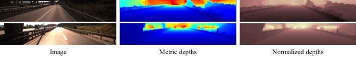
Figure 13: Metric depths and its normalized depths on KITTI.

Table 13: Comparison of depth estimation results on the Eigen split of KITTI. For each metric, the best result is boldfaced.

Method	RMSE$(\downarrow)$	$\textrm{RMSE}_{\log}(\downarrow)$	REL$(\downarrow)$	Sq REL$(\downarrow)$	$\delta_{1}(\uparrow)$	$\delta_{2}(\uparrow)$	$\delta_{3}(\uparrow)$
Fu et al. [15]	2.727	0.120	0.072	0.307	0.932	0.984	0.994
Lee et al. [28]	2.756	0.096	0.059	0.245	0.956	0.993	0.998
Yin et al. [55]	3.258	0.117	0.072	-	0.938	0.990	0.998
Lee and Kim [31]	4.512	0.176	0.115	-	0.864	0.962	0.986
Ranftl et al. [39]∗	2.573	0.092	0.062	-	0.959	0.995	0.999
Bhat et al. [3]	2.360	0.088	0.058	0.190	0.964	0.995	0.999
Patil et al. [37]	2.842	0.103	0.079	0.270	0.953	0.993	0.998
Yuan et al. [56]	2.129	0.079	0.052	0.155	0.974	0.997	0.999
Proposed	2.070	0.078	0.051	0.148	0.975	0.997	0.999

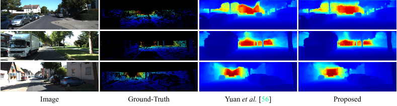
Figure 14: Qualitative comparison on KITTI.

Appendix E Relative Depth Estimation

In Table 5, we use the trained parameters of [39] and [40] from their official repositories to evaluate the generalization performance. These models use much more training images than the proposed CRDE — about 1.4M training images. For a fair comparison, we retrain [40, 39], and the proposed CRDE using the HR-WSI dataset [51], which is a relative depth dataset containing 20,378 training images. Also, we define another metric, ‘Relative RMSE,’ which computes the RMSE score between the ground truth depth map ${\mathbf{D}}$ and a calibrated depth map $\tilde{{\mathbf{R}}}$, similarly to ‘Relative $\delta_{1}$.’ Tables 14 and 15 compare relative RMSE, relative $\delta_{1}$, and Kendall’s $\tau$ results on NYUv2 and KITTI, respectively. We see that the proposed CRDE also outperforms [39] and [40] when trained with the same data.

Table 14: Comparison of relative RMSE, relative $\delta_{1}$ and Kendall’s $\tau$ results on NYUv2.

	# Params	Relative RMSE$(\downarrow)$	Relative $\delta_{1}(\uparrow)$	Kendall’s $\tau(\uparrow)$
MiDaS [40]	105.4M	0.542	0.805	0.657
DPT [39]	344.1M	0.539	0.828	0.712
CRDE	149.8M	0.455	0.874	0.737

Table 15: Comparison of relative RMSE, relative $\delta_{1}$ and Kendall’s $\tau$ results on KITTI.

	# Params	Relative RMSE$(\downarrow)$	Relative $\delta_{1}(\uparrow)$	Kendall’s $\tau(\uparrow)$
MiDaS [40]	105.4M	7.779	0.650	0.695
DPT [39]	344.1M	5.248	0.831	0.818
CRDE	149.8M	5.060	0.862	0.840

Appendix F More Analysis on FMM and R2MC

F.1 FMM

Table 16 reports the results of an ablation study on FMM components. ‘Baseline’ is the same as the one in Table 6, which is a basic encoder-decoder network using Swin transformer blocks. Note that each FMM component improves depth estimation results. Table 17 is an extended version of Table 7, which compares different combinations of mixing coefficients $\alpha,\beta,\gamma$. Note that the case of $\alpha=\beta=\gamma=1$ fails since no encoder feature is passed to the decoder. The ‘Learnable’ setting outperforms all the other settings in most cases.

Table 16: Ablation study on the components of FMMs on NYUv2.

Settings	RMSE$(\downarrow)$	REL$(\downarrow)$	$\delta_{1}(\uparrow)$	$\tau(\uparrow)$
Baseline	0.335	0.094	0.922	0.844
+ skip-connection	0.331	0.094	0.925	0.847
+ normalization	0.333	0.092	0.926	0.846
+ learnable $\alpha,\beta,\gamma$	0.330	0.092	0.926	0.848
+ R2MC	0.325	0.091	0.926	0.858

Table 17: Impacts of the hyperparameters in FMMs on NYUv2.

$\alpha$	$\beta$	$\gamma$	RMSE$(\downarrow)$	REL$(\downarrow)$	$\delta_{1}(\uparrow)$	$\tau(\uparrow)$
0	0	0	0.335	0.094	0.922	0.844
0	0	1	0.341	0.094	0.920	0.841
0	1	0	0.351	0.104	0.906	0.842
0	1	1	0.333	0.093	0.921	0.843
1	0	0	0.337	0.094	0.924	0.844
1	0	1	0.341	0.095	0.918	0.841
1	1	0	0.331	0.093	0.923	0.847
0.5	0.5	0.5	0.332	0.093	0.924	0.849
Learnable			0.330	0.092	0.926	0.848

Table 18 lists the trained values of $\alpha,\beta,\gamma$ in the proposed VDE for NYUv2. There is no clear tendency, so it is difficult to find these values manually.

Table 18: Values of $\alpha,\beta,\gamma$ after training.

	FMM1		FMM2		FMM3
Coefficient	1st	2nd	1st	2nd	1st	2nd
$\alpha$	0.4759	0.4866	0.7104	0.6753	0.5989	0.6802
$\beta$	0.4474	0.4541	0.5978	0.6129	0.4530	0.4461
$\gamma$	0.4773	0.4931	0.5092	0.4808	0.4512	0.4804

F.2 R2MC

In Table 19, we analyze the impacts of learnable matrices ${\mathbf{L}}$ in R2MCs on SUN RGB-D. Here, ‘without ${\mathbf{L}}$’ means that the value matrix ${\mathbf{V}}_{R}$ obtained from ${\mathbf{Z}}_{R}$ via self-attention is used instead of ${\mathbf{L}}$. We see that the setting ‘with ${\mathbf{L}}$’ provides better results overall, indicating that ${\mathbf{L}}$ plays the role of a camera-specific mapping function effectively.

Table 19: Impacts of learnable matrices ${\mathbf{L}}$ in R2MCs on SUN RGB-D.

Setting	Camera	RMSE$(\downarrow)$	REL $(\downarrow)$	$\delta_{1}(\uparrow)$	$\tau(\uparrow)$
without ${\mathbf{L}}$	Kinect v1	0.291	0.129	0.860	0.791
	Kinect v2	0.226	0.085	0.942	0.855
	RealSense	0.192	0.085	0.949	0.829
	Xtion	0.330	0.433	0.844	0.773
	Mean	0.254	0.142	0.898	0.811
with ${\mathbf{L}}$	Kinect v1	0.289	0.132	0.855	0.797
	Kinect v2	0.220	0.083	0.945	0.860
	RealSense	0.194	0.085	0.950	0.835
	Xtion	0.339	0.397	0.853	0.783
	Mean	0.254	0.139	0.900	0.818

Appendix G More Qualitative Results

Figures 15$\sim$24 compare versatile depth estimation results of the proposed VDE with those of ‘Separate networks.’ Figures 25, 26, and 27 compare the proposed VDE with conventional algorithms [3, 56] qualitatively on NYUv2.

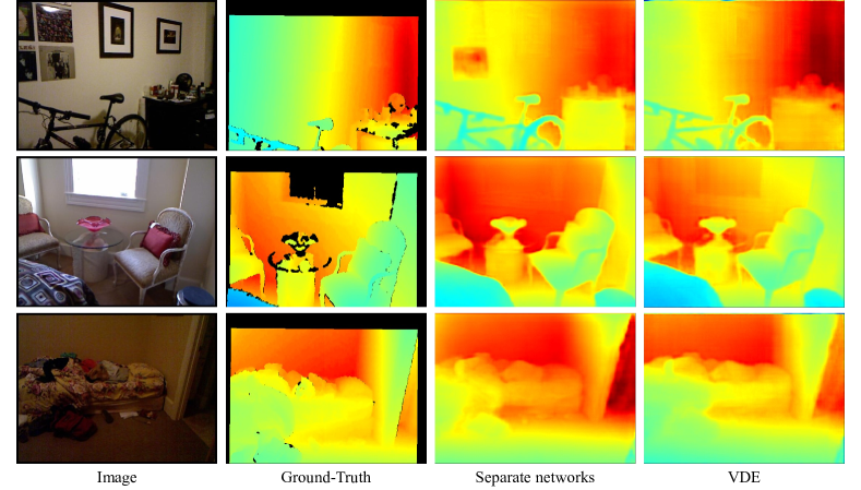
Figure 15: Versatile depth estimation reults on NYUv2.

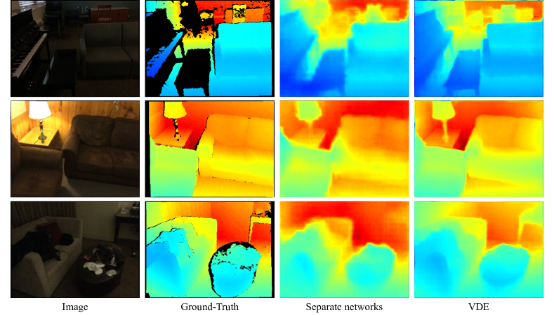
Figure 16: Versatile depth estimation reults on ScanNet.

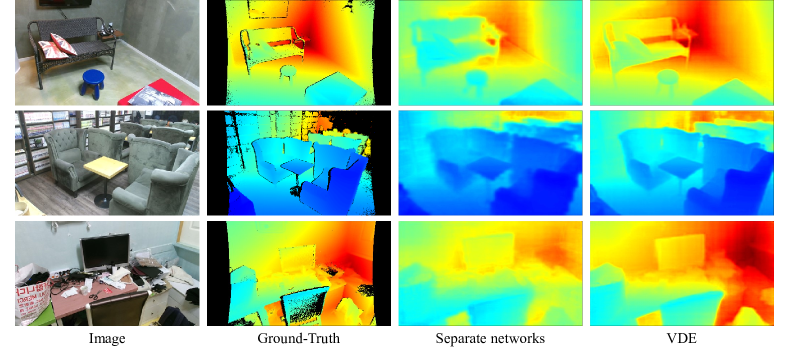
Figure 17: Versatile depth estimation reults on DIML-Indoor.

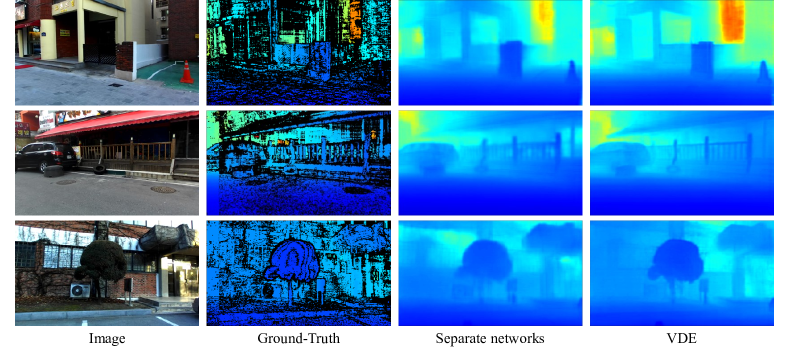
Figure 18: Versatile depth estimation reults on DIML-Outdoor.

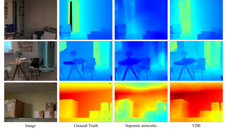
Figure 19: Versatile depth estimation reults on DIODE-Indoor.

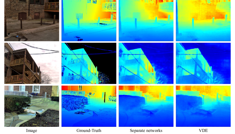
Figure 20: Versatile depth estimation reults on DIODE-Outdoor.

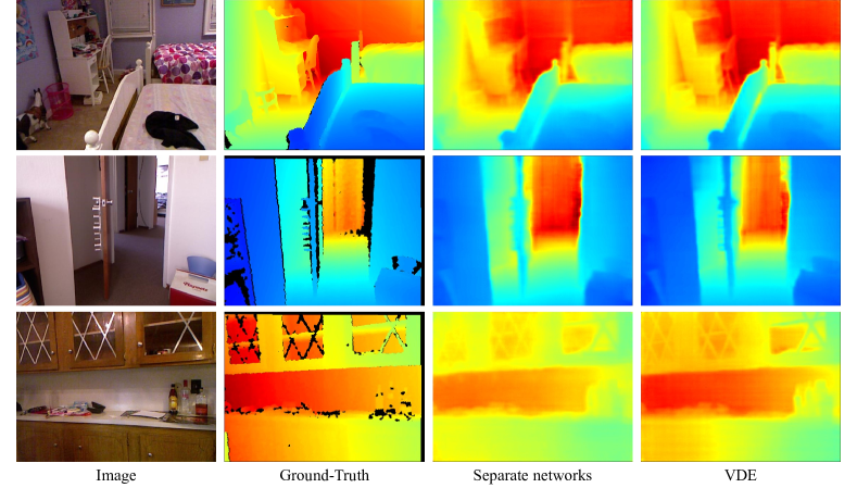
Figure 21: Versatile depth estimation reults on SUN (Kinect v1).

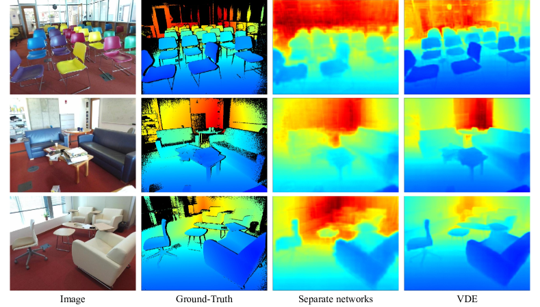
Figure 22: Versatile depth estimation reults on SUN (Kinect v2).

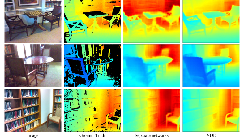
Figure 23: Versatile depth estimation reults on SUN (RealSense).

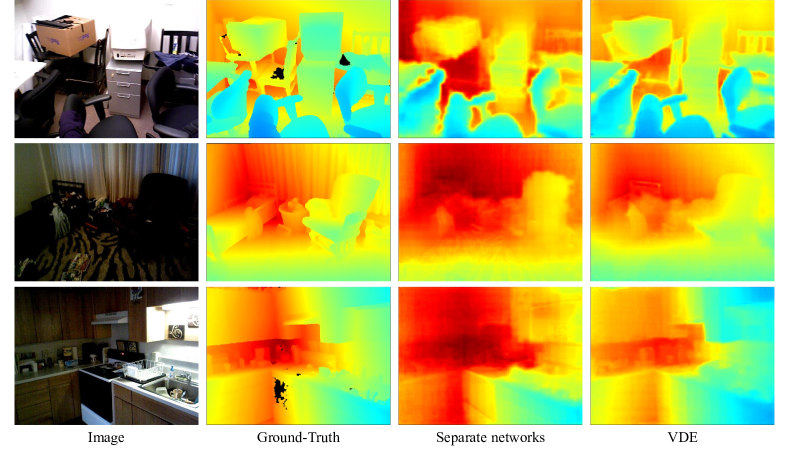
Figure 24: Versatile depth estimation reults on SUN (Xtion).

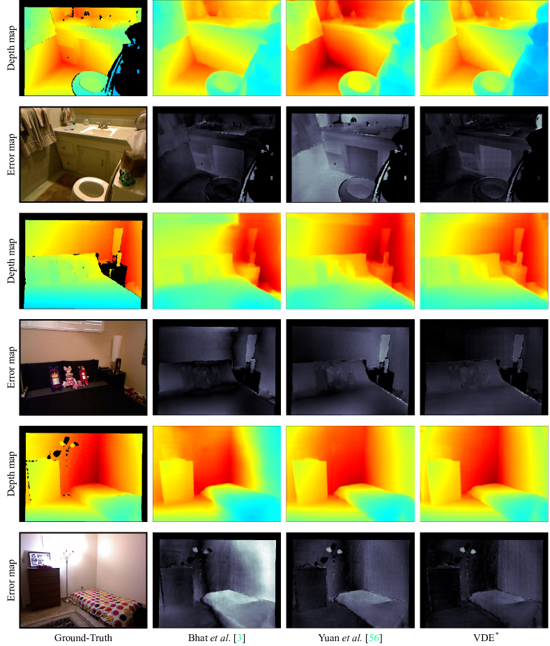
Figure 25: Qualitative comparison on NYUv2. For each depth map, the error map is also provided with a bright gray-level indicating a large error.

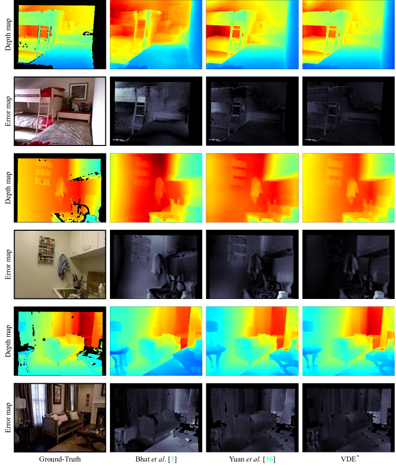
Figure 26: Qualitative comparison on NYUv2. For each depth map, the error map is also provided with a bright gray-level indicating a large error.

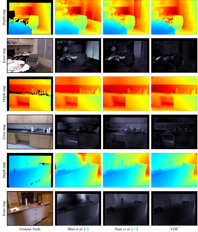
Figure 27: Qualitative comparison on NYUv2. For each depth map, the error map is also provided with a bright gray-level indicating a large error.

References

- [1] Ashutosh Agarwal and Chetan Arora. Attention attention everywhere: Monocular depth prediction with skip attention. In WACV, 2023.
- [2] Jimmy Lei Ba, Jamie Ryan Kiros, and Geoffrey E. Hinton. Layer normalization. In NeurIPS, 2016.
- [3] Shariq Farooq Bhat, Ibraheem Alhashim, and Peter Wonka. AdaBins: Depth estimation using adaptive bins. In CVPR, 2021.
- [4] Nicolas Carion, Francisco Massa, Gabriel Synnaeve, Nicolas Usunier, Alexander Kirillov, and Sergey Zagoruyko. End-to-end object detection with transformers. In ECCV, 2020.
- [5] Chun-Fu Chen, Rameswar Panda, and Quanfu Fan. RegionViT: Regional-to-local attention for vision transformers. In ICLR, 2022.
- [6] Weifeng Chen, Zhao Fu, Dawei Yang, and Jia Deng. Single-image depth perception in the wild. In NeurIPS, 2016.
- [7] Xiaotian Chen, Xuejin Chen, and Zheng-Jun Zha. Structure-aware residual pyramid network for monocular depth estimation. In IJCAI, 2019.
- [8] Bowen Cheng, Alexander G. Schwing, and Alexander Kirillov. Per-pixel classification is not all you need for semantic segmentation. In NeurIPS, 2021.
- [9] Angela Dai, Angel X. Chang, Manolis Savva, Maciej Halber, Thomas Funkhouser, and Matthias Nießner. ScanNet: Richly-annotated 3D reconstructions of indoor scenes. In CVPR, 2017.
- [10] Jacob Devlin, Ming-Wei Chang, Kenton Lee, and Kristina Toutanova. BERT: Pre-training of deep bidirectional transformers for language understanding. In NAACL, 2018.
- [11] Alexey Dosovitskiy, Lucas Beyer, Alexander Kolesnikov, Dirk Weissenborn, Xiaohua Zhai, Thomas Unterthiner, Mostafa Dehghani, Matthias Minderer, Georg Heigold, Sylvain Gelly, Jakob Uszkoreit, and Neil Houlsby. An image is worth 16x16 words: Transformers for image recognition at scale. In ICLR, 2021.
- [12] David Eigen and Rob Fergus. Predicting depth, surface normals and semantic labels with a common multi-scale convolutional architecture. In ICCV, 2015.
- [13] David Eigen, Christian Puhrsch, and Rob Fergus. Depth map prediction from a single image using a multi-scale deep network. In NeurIPS, 2014.
- [14] Jiemin Fang, Lingxi Xie, Xinggang Wang, Xiaopeng Zhang, Wenyu Liu, and Qi Tian. MSG-Transformer: Exchanging local spatial information by manipulating messenger tokens. In CVPR, 2022.
- [15] Huan Fu, Mingming Gong, Chaohui Wang, Kayhan Batmanghelich, and Dacheng Tao. Deep ordinal regression network for monocular depth estimation. In CVPR, 2018.
- [16] Andreas Geiger, Philip Lenz, and Raquel Urtasun. Are we ready for autonomous driving? the KITTI vision benchmark suite. In CVPR, 2012.
- [17] Abhinav Gupta, Alexei A. Efros, and Martial Hebert. Blocks world revisited: Image understanding using qualitative geometry and mechanics. In ECCV, 2010.
- [18] Abhinav Gupta, Martial Hebert, Takeo Kanade, and David Blei. Estimating spatial layout of rooms using volumetric reasoning about objects and surfaces. In NeurIPS, 2010.
- [19] Zhixiang Hao, Yu Li, Shaodi You, and Feng Lu. Detail preserving depth estimation from a single image using attention guided networks. In 3DV, 2018.
- [20] Minhyeok Heo, Jaehan Lee, Kyung-Rae Kim, Han-Ul Kim, and Chang-Su Kim. Monocular depth estimation using whole strip masking and reliability-based refinement. In ECCV, 2018.
- [21] Junjie Hu, Mete Ozay, Yan Zhang, and Takayuki Okatani. Revisiting single image depth estimation: Toward higher resolution maps with accurate object boundaries. In WACV, 2019.
- [22] Lam Huynh, Phong Nguyen-Ha, Jiri Matas, Esa Rahtu, and Janne Heikkilä. Guiding monocular depth estimation using depth-attention volume. In ECCV, 2020.
- [23] Jinyoung Jun, Jae-Han Lee, Chul Lee, and Chang-Su Kim. Depth map decomposition for monocular depth estimation. In ECCV, 2022.
- [24] Maurice G. Kendall. A new measure of rank correlation. Biometrika, 30(1/2):81–93, 1938.
- [25] Youngjung Kim, Hyungjoo Jung, Dongbo Min, and Kwanghoon Sohn. Deep monocular depth estimation via integration of global and local predictions. IEEE Trans. Image Process., 27(8):4131–4144, 2018.
- [26] Diederik P. Kingma and Jimmy Ba. Adam: A method for stochastic optimization. In ICLR, 2015.
- [27] Iro Laina, Christian Rupprecht, Vasileios Belagiannis, Federico Tombari, and Nassir Navab. Deeper depth prediction with fully convolutional residual networks. In 3DV, 2016.
- [28] Jin Han Lee, Myung-Kyu Han, Dong Wook Ko, and Il Hong Suh. From big to small: Multi-scale local planar guidance for monocular depth estimation. arXiv preprint arXiv:1907.10326, 2019.
- [29] Jae-Han Lee, Minhyeok Heo, Kyung-Rae Kim, and Chang-Su Kim. Single-image depth estimation based on Fourier domain analysis. In CVPR, 2018.
- [30] Jae-Han Lee and Chang-Su Kim. Monocular depth estimation using relative depth maps. In CVPR, 2019.
- [31] Jae-Han Lee and Chang-Su Kim. Multi-loss rebalancing algorithm for monocular depth estimation. In ECCV, 2020.
- [32] Anat Levin, Dani Lischinski, and Yair Weiss. Colorization using optimization. ACM Trans. Graph., 23(3):689–694, 2004.
- [33] Zhengqi Li, Tali Dekel, Forrester Cole, Richard Tucker, Noah Snavely, Ce Liu, and William T. Freeman. Learning the depths of moving people by watching frozen people. In CVPR, 2019.
- [34] Zhengqi Li and Noah Snavely. MegaDepth: Learning single-view depth prediction from internet photos. In CVPR, 2018.
- [35] Julian Lienen, Eyke Hüllermeier, Ralph Ewerth, and Nils Nommensen. Monocular depth estimation via listwise ranking using the Plackett-Luce model. In CVPR, 2021.
- [36] Ze Liu, Yutong Lin, Yue Cao, Han Hu, Yixuan Wei, Zheng Zhang, Stephen Lin, and Baining Guo. Swin Transformer: Hierarchical vision transformer using shifted windows. In ICCV, 2021.
- [37] Vaishakh Patil, Christos Sakaridis, Alexander Liniger, and Luc Van Gool. P3Depth: Monocular depth estimation with a piecewise planarity prior. In CVPR, 2022.
- [38] Michaël Ramamonjisoa and Vincent Lepetit. SharpNet: Fast and accurate recovery of occluding contours in monocular depth estimation. In ICCVW, 2019.
- [39] René Ranftl, Alexey Bochkovskiy, and Vladlen Koltun. Vision transformers for dense prediction. In ICCV, 2021.
- [40] René Ranftl, Katrin Lasinger, David Hafner, Konrad Schindler, and Vladlen Koltun. Towards robust monocular depth estimation: Mixing datasets for zero-shot cross-dataset transfer. IEEE Trans. Pattern Anal. Mach. Intell., 44(3):1623–1637, 2020.
- [41] Olaf Ronneberger, Philipp Fischer, and Thomas Brox. U-Net: Convolutional networks for biomedical image segmentation. In MICCAI, 2015.
- [42] Ashutosh Saxena, Min Sun, and Andrew Y. Ng. Make3D: Learning 3D scene structure from a single still image. IEEE Trans. Pattern Anal. Mach. Intell., 31(5):824–840, 2008.
- [43] Meng-Li Shih, Shih-Yang Su, Johannes Kopf, and Jia-Bin Huang. 3D photography using context-aware layered depth inpainting. In CVPR, 2020.
- [44] Nathan Silberman, Derek Hoiem, Pushmeet Kohli, and Rob Fergus. Indoor segmentation and support inference from RGBD images. In ECCV, 2012.
- [45] Shuran Song, Samuel P Lichtenberg, and Jianxiong Xiao. SUN RGB-D: A RGB-D scene understanding benchmark suite. In CVPR, 2015.
- [46] Igor Vasiljevic, Nick Kolkin, Shanyi Zhang, Ruotian Luo, Haochen Wang, Falcon Z. Dai, Andrea F. Daniele, Mohammadreza Mostajabi, Steven Basart, Matthew R. Walter, and Gregory Shakhnarovich. DIODE: A dense indoor and outdoor depth dataset. arXiv preprint arXiv:1908.00463, 2019.
- [47] Ashish Vaswani, Noam Shazeer, Niki Parmar, Jakob Uszkoreit, Llion Jones, Aidan N. Gomez, Łukasz Kaiser, and Illia Polosukhin. Attention is all you need. In NeurIPS, 2017.
- [48] Chaoyang Wang, Simon Lucey, Federico Perazzi, and Oliver Wang. Web stereo video supervision for depth prediction from dynamic scenes. In 3DV, 2019.
- [49] Peng Wang, Xiaohui Shen, Zhe Lin, Scott Cohen, Brian Price, and Alan Yuille. Towards unified depth and semantic prediction from a single image. In CVPR, 2015.
- [50] Ke Xian, Chunhua Shen, Zhiguo Cao, Hao Lu, Yang Xiao, Ruibo Li, and Zhenbo Luo. Monocular relative depth perception with web stereo data supervision. In CVPR, 2018.
- [51] Ke Xian, Jianming Zhang, Oliver Wang, Long Mai, Zhe Lin, and Zhiguo Cao. Structure-guided ranking loss for single image depth prediction. In CVPR, 2020.
- [52] Dan Xu, Elisa Ricci, Wanli Ouyang, Xiaogang Wang, and Nicu Sebe. Multi-scale continuous CRFs as sequential deep networks for monocular depth estimation. In CVPR, 2017.
- [53] Guanglei Yang, Hao Tang, Mingli Ding, Nicu Sebe, and Elisa Ricci. Transformer-based attention networks for continuous pixel-wise prediction. In ICCV, 2021.
- [54] Mao Ye, Xianwang Wang, Ruigang Yang, Liu Ren, and Marc Pollefeys. Accurate 3D pose estimation from a single depth image. In ICCV, 2011.
- [55] Wei Yin, Yifan Liu, Chunhua Shen, and Youliang Yan. Enforcing geometric constraints of virtual normal for depth prediction. In ICCV, 2019.
- [56] Weihao Yuan, Xiaodong Gu, Zuozhuo Dai, Siyu Zhu, and Ping Tan. NewCRFs: Neural window fully-connected CRFs for monocular depth estimation. In CVPR, 2022.
- [57] Hengshuang Zhao, Jianping Shi, Xiaojuan Qi, Xiaogang Wang, and Jiaya Jia. Pyramid scene parsing network. In CVPR, 2017.
- [58] Daniel Zoran, Phillip Isola, Dilip Krishnan, and William T. Freeman. Learning ordinal relationships for mid-level vision. In ICCV, 2015.