Refined product formulas for Tamari intervals

Abstract.

We provide short product formulas for the $f$-vectors of the canonical complexes of the Tamari lattices and of the cellular diagonals of the associahedra.

Introduction

Consider the Tamari lattice $\mathrm{Tam}(n)$, whose elements are the binary trees with $n$ nodes, and whose cover relations are given by right rotations [Tam51]. For a binary tree $T$, we denote by $\operatorname{des}(T)$ (resp. by $\operatorname{asc}(T)$) the number of binary trees covered by $T$ (resp. covering $T$) in the Tamari lattice. In other words, if we label its nodes in inorder and orient its edges towards its root, then $\operatorname{des}(T)$ (resp. $\operatorname{asc}(T)$) is the number of edges $i\to j$ in $T$ with $i>j$ (resp. with $i<j$). The purpose of this paper is to prove the following two surprising formulas, whose first few values are gathered in Tables 1 and 2.

Theorem 1.

For any $n,k\in\mathbb{N}$, the number $a_{n,k}$ of intervals $S\leq T$ of the Tamari lattice $\mathrm{Tam}(n)$ such that $\operatorname{des}(S)+\operatorname{asc}(T)=k$ is given by

$$a_{n,k}=\frac{2}{n(n+1)}\binom{n+1}{k+2}\binom{3n}{k}.$$

Theorem 2.

For any $n,k\in\mathbb{N}$, the sum $b_{n,k}$ of the binomial coefficients $\binom{\operatorname{des}(S)+\operatorname{asc}(T)}{k}$ over all intervals $S\leq T$ of the Tamari lattice $\mathrm{Tam}(n)$ is given by

$$b_{n,k}=\sum_{\ell=k}^{n-1}a_{n,\ell}\binom{\ell}{k}=\frac{2}{(3n+1)(3n+2)}\binom{n-1}{k}\binom{4n+1-k}{n+1}.$$

$n\backslash k$	$0$	$1$	$2$	$3$	$4$	$5$	$6$	$7$	$8$	$\Sigma$
$1$	$1$									$1$
$2$	$1$	$2$								$3$
$3$	$1$	$6$	$6$							$13$
$4$	$1$	$12$	$33$	$22$						$68$
$5$	$1$	$20$	$105$	$182$	$91$					$399$
$6$	$1$	$30$	$255$	$816$	$1020$	$408$				$2530$
$7$	$1$	$42$	$525$	$2660$	$5985$	$5814$	$1938$			$16965$
$8$	$1$	$56$	$966$	$7084$	$24794$	$42504$	$33649$	$9614$		$118668$
$9$	$1$	$72$	$1638$	$16380$	$81900$	$215280$	$296010$	$197340$	$49335$	$857956$

Table 1. The first few values of $a_{n,k}=\frac{2}{n(n+1)}\binom{n+1}{k+2}\binom{3n}{k}$. Note that the first column is $1$, the second column is $n(n-1)$ [OEI10, A002378], the last three diagonals are [OEI10, A004321], [OEI10, A006630], and [OEI10, A000139], and the column sum is [OEI10, A000260]. The $n$th row gives the $f$-vector of the canonical complex of the Tamari lattice $\mathrm{Tam}(n)$.

$n\backslash k$	$0$	$1$	$2$	$3$	$4$	$5$	$6$	$7$	$8$
$1$	$1$
$2$	$3$	$2$
$3$	$13$	$18$	$6$
$4$	$68$	$144$	$99$	$22$
$5$	$399$	$1140$	$1197$	$546$	$91$
$6$	$2530$	$9108$	$12903$	$8976$	$3060$	$408$
$7$	$16965$	$73710$	$131625$	$123500$	$64125$	$17442$	$1938$
$8$	$118668$	$604128$	$1302651$	$1540770$	$1078539$	$446292$	$100947$	$9614$
$9$	$857956$	$5008608$	$12660648$	$18086640$	$15958800$	$8898240$	$3058770$	$592020$	$49335$

Table 2. The first few values of $b_{n,k}=\frac{2}{(3n+1)(3n+2)}\binom{n-1}{k}\binom{4n+1-k}{n+1}$. Note that the first column is [OEI10, A000260] while the diagonal is [OEI10, A000139]. The $n$th row gives the $f$-vector of the cellular diagonal of the $(n-1)$-dimensional associahedron.

These formulas are of interest for several reasons. First, we will observe in Section 1 that these formulas count the faces of two complexes defined from the Tamari lattice and the associahedron:

1. Canonical complex of the Tamari lattice. The canonical complex of a semidistributive lattice $L$ is a flag simplicial complex which encodes each interval $s\leq t$ of $L$ by recording the canonical join representation of $s$ together with the canonical meet representation of $t$ [Rea15, Bar19, AP22]. The dimension of the simplex corresponding to an interval $s\leq t$ is precisely the number of elements covered by $s$ plus the number of elements covering $t$. The $f$-vector of the canonical complex of the Tamari lattice is thus the vector $(a_{n,k})_{0\leq k<n}$ (Section 1.1). The canonical complex of the weak order was studied in details in [AP22], and its $f$-vector was discussed in [AP22, Rem. 43]. The canonical complex of the Tamari lattice is an induced subcomplex of the canonical complex of the weak order but was not specifically considered in [AP22].

2. Cellular diagonal of the associahedron. The associahedron is a polytope whose graph is isomorphic to the rotation graph on binary trees. In fact, the oriented graph of the realization of [Lod04, SS93] is isomorphic to the Hasse diagram of the Tamari lattice. The cellular diagonal of the associahedron is a polytopal complex covering the associahedron, crucial in homotopy theory [SU04, MS06, Lod11, MTTV21, LA22]. The faces of this complex correspond to the pairs of faces of the associahedron given by the so-called magical formula: a pair $(F,G)$ of faces belongs to the cellular diagonal if and only if $\max(F)\leq\min(G)$ (where $\leq$, $\max$ and $\min$ refer to the order given by the Tamari lattice). The $f$-vector of this complex is thus the vector $(b_{n,k})_{0\leq k<n}$ (Section 1.2).

Second, we can already observe that these formulas have some relevant specializations:

1. The Tamari intervals are enumerated by

   $$\sum_{\ell=0}^{n-1}a_{n,\ell}=b_{n,0}=\frac{2}{(3n+1)(3n+2)}\binom{4n+1}{n+1}.$$

   This formula was proved in [Cha07] and appears as [OEI10, A000260]. It also counts the rooted $3$-connected planar triangulations with $2n+2$ faces, and an explicit bijection between Tamari intervals and $3$-connected triangulations was given in [BB09].

2. The synchronized Tamari intervals are enumerated by

   $$a_{n,n-1}=\frac{2}{n(n+1)}\binom{3n}{n-1}=\frac{2}{(n+1)(2n+1)}\binom{3n}{n}=\frac{2}{(3n+1)(3n+2)}\binom{3n+2}{n+1}=b_{n,n-1}.$$

   This formula was proved in [FPR17] and appears as [OEI10, A000139]. It also counts the rooted non-separable planar maps with $n+1$ edges, and the $2$-stack sortable permutations of $[n]$, among others.

(There obviously are some other specializations, like $a_{n,0}=1$, $a_{n,1}=n(n-1)$ [OEI10, A002378], $a_{n,n-3}=\binom{3n}{n-3}$ [OEI10, A004321], and $a_{n,n-2}=\frac{2}{n}\binom{3n}{n-2}$ [OEI10, A006630], but they are less relevant for our purposes). We will see in Section 6.1.3 that the statistics $\operatorname{des}(S)$ and $\operatorname{asc}(T)$ are transported via the bijection of [BB09] to natural statistics in terms of Schnyder woods of rooted triangulations, leading to an interpretation of the numbers $a_{n,k}$ in terms of maps. In contrast, we are not aware of other combinatorial interpretations of our formula $b_{n,k}$ for arbitrary $n$ and $k$, in particular in the world of maps.

We present three analytic proofs of Theorems 1 and 2 in Sections 2, LABEL:, 3, LABEL:, 4, LABEL: and 5. These three proofs use generating functionology [FS09], following the methodology already introduced and exploited in [Cha07, Cha18]. We show in Section 2 that a natural recursive decomposition of Tamari intervals yields a quadratic equation on the generating function of Tamari intervals with one additional catalytic variable. Using the quadratic method [GJ04], this quadratic equation can be transformed into a polynomial equation on the generating function $A(t,z)\mbox{\,\raisebox{0.86108pt}{\scriptsize$\mathrm{:}$}$=$\,}\sum a_{n,k}t^{n}z^{k}$. At this point, we describe three methods to derive Theorems 1 and 2 from this polynomial equation:

• In Section 3, we take advantage of two interesting coincidences. Namely, we first prove Theorem 1 by extraction of the coefficients of $A(t,z)$ by Lagrange inversion after an adequate reparametrization of our polynomial equation (Section 3.1). We then prove that Theorem 1 implies Theorem 2 using a simple binomial identity (Section 3.2).

• In Section 4, we use a more robust method, based on recurrence relations obtained by creative telescoping. We observe that Theorem 1 (Section 4.1), Theorem 2 (Section 4.2), and our binomial identity (Section 4.3) can all be systematically obtained by this method.

• In Section 5, we observe that a holonomic differential system annihilating $A(t,z)$ is available effortlessly, inducing that a holonomic recurrence system annihilating its bivariate coefficient sequence $([t^{n}z^{k}]A(t,z))_{(n,k)\in\mathbb{Z}^{2}}$ can be derived as well. We then simplify and solve the system for its bivariate hypergeometric solutions, thus proving Theorem 1. Unfortunately, we could not obtain Theorem 2 by the same approach.

We then present bijective considerations on Theorems 1 and 2. We first present some statistics equivalent to $\operatorname{des}(S)$ and $\operatorname{asc}(T)$ (Section 6.1), expressed in terms of canopy agreements in binary trees (Section 6.1.1), of valleys and double falls in Dyck paths (Section 6.1.2), and of internal degrees of Schnyder woods in maps (Section 6.1.3). These bijections were used in [FH19] to obtain a simple expression for the generating function of Tamari intervals with variables recording the canopy patterns of the two trees. We use this expression to derive directly Theorem 1 from Lagrange inversion (Section 6.2). We note that an even simpler bijective approach can be obtained from the recent direct bijection of [FFN23] between Tamari intervals and blossoming trees. Details will appear in [FFN23].

Finally, we conclude the paper with some additional observations concerning Theorems 1 and 2 in Section 7. We first discuss the (im)possibility to refine our formulas (Section 7.1), either by adding the additional statistics used for the catalytic variable (Section 7.1.1), or by separating the statistics $\operatorname{des}(S)$ and $\operatorname{asc}(T)$ (Section 7.1.2). We then provide a formula for the number of internal faces of the cellular diagonal of the associahedron (Section 7.2) which specializes on the one hand to the number of new Tamari intervals and on the other hand to the number of synchronized Tamari intervals of [Cha07]. We then discuss the problem to extend our results to $m$-Tamari lattice (Section 7.3). We conclude with an observation concerning decompositions of the cellular diagonal of the associahedron (Section 7.4).

A companion worksheet is available at https://mathexp.eu/chyzak/tamari/: it provides all calculations in the present article, performed by the computer-algebra system Maple.

1. Canonical complex of the Tamari lattice and diagonal of the associahedron

In this section, we interpret the numbers $a_{n,k}$ in terms of the canonical complex of the Tamari lattice (Section 1.1) and the numbers $b_{n,k}$ in terms of the cellular diagonal of the associahedron (Section 1.2). These two interpretations are our motivations to study $a_{n,k}$ and $b_{n,k}$, but are not used beyond this section. Rather than giving all details of the definitions of these objects, we thus prefer to refer to the original articles and only gather the essential material to make the connection.

1.1. Canonical complex of the Tamari lattice

A lattice $(L,\leq,\wedge,\vee)$ is join semidistributive when $x\vee y=x\vee z$ implies $x\vee(y\wedge z)=x\vee y$. Any $x\in L$ then admits a canonical join representation, which is a minimal irredundant representation $x=\bigvee J$ (for the order $J\leq J^{\prime}$ if for any $j\in J$, there is $j^{\prime}\in J^{\prime}$ with $j\leq j^{\prime}$). The canonical join complex [Rea15, Bar19] of a join semidistributive lattice $L$ is the simplicial complex of canonical join representations of the elements of $L$. Note that the dimension of the face of the canonical complex corresponding to an element $x$ of $L$ is the size of its canonical join representation, which is the number of elements covered by $x$ in $L$. We define dually meet semidistributive lattices and their canonical meet complexes, and say that $L$ is semidistributive when it is both join and meet semidistributive. The canonical complex [AP22] of a semidistributive lattice $L$ is the simplicial complex whose faces are $J\sqcup M$ where $x=\bigvee J$ is the canonical join representation and $y=\bigwedge M$ is the canonical meet representation for an interval $x\leq y$ in $L$. Note that the dimension of the face of the canonical complex corresponding to an interval $x\leq y$ is the number of elements covered by $x$ in $L$ plus the number of elements covering $y$ in $L$. Observe also that the canonical complex is flag, meaning that it is the clique complex of its graph.

Example 3.

The Tamari lattice is semidistributive. Its join (resp. meet) irreducible elements are given by binary trees $T$ with $\operatorname{des}(T)=1$ (resp. with $\operatorname{asc}(T)=1$), i.e. with a single right (resp. left) edge. Such a tree is made by glueing two left (resp. right) combs along a right (resp. left) edge, and can thus be encoded by an arc. The canonical join (resp. meet) representation of a binary tree $T$ is a non-crossing arc diagram with one arc for each right (resp. left) edge of $T$, which is also known as the non-crossing partition corresponding to $T$. Moreover, for a Tamari interval $S\leq T$, an arc $j$ of the canonical join representation of $S$ can cross an arc $m$ of the canonical meet representation of $T$ only if $j$ passes from above to below $m$. The canonical complex of the Tamari lattice is thus called the semi-crossing complex. This complex was extensively studied in [AP22] (note that the canonical complex of the Tamari lattice is just the restriction to down arcs of the canonical complex of the weak order which was the one actually studied in [AP22]). It is illustrated in Figure 1. The top left picture shows the Tamari lattice where in each binary tree, the descents are colored red, and the ascents are colored blue. The middle left picture is the translation on arcs, obtained by flattening each tree to the horizontal line. The bottom left picture is the semi-crossing complex, thus the canonical complex of the Tamari lattice when $n=3$ (note that it has indeed $13$ faces: the empty set, $6$ vertices, and $6$ edges). The right picture is the semi-crossing complex, thus the canonical complex of the Tamari lattice when $n=4$ (note that it has indeed $68$ faces: the empty set, $12$ vertices, $33$ edges, and $22$ triangles). Note that we only draw the graphs of the canonical complexes, since they are flag simplicial complexes.

 

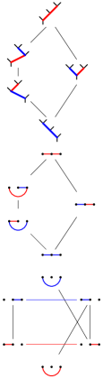
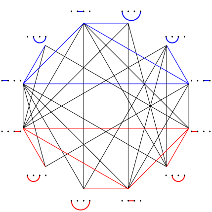
Figure 1. The canonical complex of the Tamari lattice. Left: The Tamari lattice $\mathrm{Tam}(2)$ seen on binary trees (top) and on semi-crossing arc bidiagrams (middle), and the canonical complex of $\mathrm{Tam}(2)$ (bottom), with $f$-vector $(1,6,6)$. Right: The canonical complex of $\mathrm{Tam}(3)$, with $f$-vector $(1,12,33,22)$.

We are now ready to observe the connection between the numbers $a_{n,k}$ of Theorem 1 and the $f$-vector of the canonical complex of the Tamari lattice. Recall that the $f$-vector of a $d$-dimensional polytopal complex of $\mathcal{C}$ is the vector $(f_{0},f_{1},\dots,f_{d})$ where $f_{i}$ denotes the number of $i$-dimensional faces of $\mathcal{C}$.

Proposition 4.

The $f$-vector of the canonical complex of the Tamari lattice $\mathrm{Tam}(n)$ on binary trees with $n$ nodes is given by $(a_{n,k})_{0\leq k<n}.$

Proof.

The dimension of the face of the canonical complex of the Tamari lattice corresponding to an interval $S\leq T$ is the number of binary trees covered by $S$ plus the number of binary trees covering $T$, which is precisely $\operatorname{des}(S)+\operatorname{asc}(T)$. Hence, the number of $k$-dimensional faces of the canonical complex of $\mathrm{Tam}(n)$ is given by $a_{n,k}$. ∎

1.2. Diagonal of the associahedron

The diagonal of a polytope $P$ is the map $\delta:P\to P\times P$ defined by $x\mapsto(x,x)$. A cellular approximation of the diagonal of $P$ (or just cellular diagonal of $P$ for short) is a map $\tilde{\delta}:P\to P\times P$ homotopic to $\delta$, which agrees with $\delta$ on the vertices of $P$, and whose image is a union of faces of $P\times P$. For a family of polytopes whose faces are products of polytopes in the family (like simplices, cubes, permutahedra or associahedra among others), some algebraic purposes additionally require the cellular diagonal to be compatible with the face structure. Finding cellular diagonals in such families of polytopes is a difficult and important challenge at the crossroad of operad theory, homotopical algebra, combinatorics and discrete geometry, see [SU04, MS06, Lod11, MTTV21, LA22] and the references therein.

Here, we focus on the associahedra. Algebraic diagonals for the associahedra were found in [SU04] and later in [MS06, Lod11]. The first topological diagonal for the associahedra, as defined above, was given in [MTTV21] for the realizations of the associahedra of [Lod04, SS93]. It recovers, at the cellular level, all the previous formulas [SU22, DOJVLA⁺23]. We simply denote by $\Delta_{d}$ the cellular diagonal of the $d$-dimensional associahedron of [Lod04, SS93] constructed in [MTTV21]. The faces of $\Delta_{d}$ are given by the following description, called the magical formula.

Proposition 5 ([MTTV21, Thm. 2]).

The $k$-dimensional faces of the cellular diagonal $\Delta_{d}$ correspond to the pairs $(F,G)$ of faces of the associahedron with

$$\dim(F)+\dim(G)=k\qquad\text{and}\qquad\max(F)\leq\min(G)$$

where $\leq$, $\max$ and $\min$ refer to the order given by the Tamari lattice.

The method of [MTTV21], fully developed in [LA22] relies on the theory of fiber polytopes of [BS92]. It enables to see the cellular diagonal of the associahedron as a polytopal complex refining the associahedron, a point of view we shall adopt in our figures for the rest of the paper.

Example 6.

The cellular diagonal $\Delta_{2}$ is illustrated in Figure 2. The left picture is the $2$-dimensional associahedron, with faces labeled by Schröder trees (the colors depend on the dimension), and in particular with vertices labeled by binary trees. The middle picture is the cellular diagonal $\Delta_{2}$ seen as a polyhedral complex refining the $2$-dimensional associahedron, with faces labeled by pairs $(F,G)$ of Schröder trees, and in particular with vertices labeled by Tamari intervals. The right picture is a decomposition of $\Delta_{2}$, where each face $(F,G)$ is associated to the Tamari interval ${\max(F)\leq\min(G)}$. In other words, the Tamari interval associated to a pair $(F,G)$ of Schröder trees is obtained by replacing each $p$-ary node of $F$ (resp. of $G$) by a right (resp. left) comb with $p$ leaves. For each Tamari interval $S\leq T$, we have colored in red (resp. blue) the edges of $S$ (resp. of $T$) corresponding to descents of $S$ (resp. to ascents of $T$).

We are now ready to observe the connection between the numbers $b_{n,k}$ of Theorem 2 and the $f$-vector of the cellular diagonal of the $(n-1)$-dimensional associahedron.

Proposition 7.

The $f$-vector of the cellular diagonal $\Delta_{n-1}$ of the $(n-1)$-dimensional associahedron is given by $(b_{n,k})_{0\leq k<n}.$

Proof.

For each binary tree $T$, there are precisely $\binom{\operatorname{des}(T)}{\ell}$ (resp. $\binom{\operatorname{asc}(T)}{\ell}$) $\ell$-dimensional faces of the associahedron whose maximal (resp. minimal) vertex is $T$, because the associahedron is a simple polytope. We thus directly derive from the magical formula of Proposition 5 that the number of $k$-dimensional faces of $\Delta_{n-1}$ is

$$\sum_{S\leq T}\sum_{0\leq\ell\leq k}\binom{\operatorname{des}(S)}{\ell}\binom{\operatorname{des}(T)}{k-\ell}=\sum_{S\leq T}\binom{\operatorname{des}(S)+\operatorname{asc}(T)}{k}=b_{n,k}.\qed$$

Remark 8.

This proof can also be interpreted on Figure 2. Namely, by attaching each face $(F,G)$ to the Tamari interval $\max(F)\leq\min(G)$, we have partitioned the face poset of $\Delta_{n-1}$ into boolean lattices based at its vertices. As the boolean lattice attached to a Tamari interval $S\leq T$ has rank $\operatorname{des}(S)+\operatorname{asc}(T)$, we obtain that the number of $k$-dimensional faces in this part of the face poset is $\binom{\operatorname{des}(S)+\operatorname{asc}(T)}{k}$. We will discuss other possible decompositions of $\Delta_{n-1}$ in Section 7.4.

Figure 2. Left: The $2$-dimensional associahedron with its faces labeled by Schröder trees with $4$ leaves (in particular, its vertices correspond to binary trees). Middle: The cellular diagonal $\Delta_{2}$ with its faces labeled by pairs of Schröder trees given by the magical formula (in particular, its vertices correspond to Tamari intervals). Right: The decomposition of the cellular diagonal $\Delta_{2}$ obtained by associating each face $(F,G)$ to the Tamari interval $\max(F)\leq\min(G)$. The $f$-vector is $(13,18,6)$.

Remark 9.

In view of the previous remark, it is natural to call $(a_{n,k})_{0\leq k<n}$ the $h$-vector of $\Delta_{n-1}$. In particular, the vectors $(a_{n,k})_{0\leq k<n}$ and $(b_{n,k})_{0\leq k<n}$ are related by the same binomial transform as the $f$- and $h$-vectors of a simple polytope. See also Lemma 21.

Remark 10.

Note that the lattice structures can be read on the geometric realizations:

• The graph of the associahedron, oriented from the left comb to the right comb, is the Hasse diagram of the Tamari lattice.

• The graph of the cellular diagonal $\Delta_{d}$, oriented from the pair of left combs to the pair of right combs, is the Hasse diagram of the lattice of Tamari intervals.

See Figure 2, where the graphs should be oriented from bottom to top. In this paper, we do not use the fact that these posets are actually lattices.

2. Grafting decompositions

In this section, we obtain a polynomial equation satisfied by the generating function $A(t,z)\mbox{\,\raisebox{0.86108pt}{\scriptsize$\mathrm{:}$}$=$\,}\sum a_{n,k}t^{n}z^{k}$, that will be exploited in Sections 3, LABEL:, 4, LABEL: and 5 to derive Theorems 1 and 2. Following the approach of [Cha07, Cha18], we use a standard decomposition of Tamari intervals that naturally introduces an additional catalytic variable.

We denote by $S/S^{\prime}$ (resp. by $S^{\prime}\backslash S$) the binary tree obtained by grafting the root of $S$ on the leftmost (resp. rightmost) leaf of $S^{\prime}$. A grafting decomposition of $S$ is an expression ${S=S_{0}/S_{1}/\dots/S_{k}}$ where $S_{i}$ is a binary tree with at least a node. In other words, a grafting decomposition of $S$ is obtained by cutting some of the edges of $S$ along the path from its root to its leftmost leaf. See Figure 3. For a binary tree $T$, we denote by $n(T)$ the number of nodes of $T$ and by $\ell(T)$ the number of edges along the path from its root to its leftmost leaf (here, we only count edges between two nodes). To fix the ideas, $n(Y)=1$ and $\ell(Y)=0$ for the unique binary tree $Y$ with a single node (and thus two leaves). The following observations were made in [Cha07, Sect. 3] and [Cha18, Sect. 3.1], and are illustrated in Figure 4.

Lemma 11 ([Cha07, Cha18]).

.

1. Assume that $S=S_{0}/S_{1}/\dots/S_{k}$ and $T=T_{0}/T_{1}/\dots/T_{k}$ are such that $n(S_{i})=n(T_{i})$ for all $i\in[k]$. Then $S\leq T$ if and only if $S_{i}\leq T_{i}$ for all $i\in[k]$.

2. If $S\leq T$, then we can write $S=S_{0}/S_{1}/\dots/S_{\ell}$ and $T=T_{0}/T_{1}/\dots/T_{\ell}$ where $\ell=\ell(T)$ and $n(S_{i})=n(T_{i})$ for all $i\in[\ell]$.

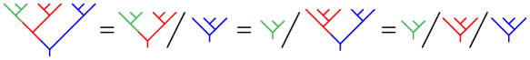
Figure 3. All grafting decompositions of a binary tree.

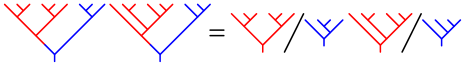
Figure 4. A grafting decomposition of a Tamari interval.

Consider now the generating function

$$\mathbb{A}(u,v,t,z)\mbox{\,\raisebox{0.86108pt}{\scriptsize$\mathrm{:}$}$=$\,}\sum_{S\leq T}u^{\ell(S)}v^{\ell(T)}t^{n(S)}z^{\operatorname{des}(S)+\operatorname{asc}(T)},$$

where the sum ranges over all Tamari intervals (with arbitrary many nodes). To simplify notations, we abbreviate $A_{u}\mbox{\,\raisebox{0.86108pt}{\scriptsize$\mathrm{:}$}$=$\,}A_{u}(t,z)\mbox{\,\raisebox{0.86108pt}{\scriptsize$\mathrm{:}$}$=$\,}\mathbb{A}(u,1,t,z)$ and $A^{\circ}_{u}\mbox{\,\raisebox{0.86108pt}{\scriptsize$\mathrm{:}$}$=$\,}A^{\circ}_{u}(t,z)\mbox{\,\raisebox{0.86108pt}{\scriptsize$\mathrm{:}$}$=$\,}\mathbb{A}(u,0,t,z)$. Note that

$$A_{1}(t,z)\mbox{\,\raisebox{0.86108pt}{\scriptsize$\mathrm{:}$}$=$\,}\mathbb{A}(1,1,t,z)=A(t,z).$$

Observe also that $A^{\circ}_{u}(t,z)$ is the generating function of indecomposable Tamari intervals, i.e. of Tamari intervals $S\leq T$ where $\ell(T)=0$ so that the decomposition of Lemma 11 (ii) is trivial. Lemma 11 leads to the following functional equation connecting $A_{u}$ and $A_{1}$.

Proposition 12.

The generating functions $A_{u}\mbox{\,\raisebox{0.86108pt}{\scriptsize$\mathrm{:}$}$=$\,}\mathbb{A}(u,1,t,z)$ and $A_{1}\mbox{\,\raisebox{0.86108pt}{\scriptsize$\mathrm{:}$}$=$\,}\mathbb{A}(1,1,t,z)$ satisfy the quadratic functional equation

$$(u-1)A_{u}=t\big{(}u-1+u(u+z-1)A_{u}-zA_{1}\big{)}\big{(}1+uzA_{u}\big{)}.$$

Proof.

This statement could be directly deduced by substituing $x=1$ and $y=\bar{y}=z$ in the equation given in [Cha18, Prop. 1]. For completeness, we prefer to transpose the proof as we need a much simpler version of the proof of [Cha18, Prop. 1].

By definition, any Tamari interval $S\leq T$ is either indecomposable or can be decomposed as ${S=S^{\prime}/S^{\prime\prime}}$ and $T=T^{\prime}/T^{\prime\prime}$ for an indecomposable Tamari interval $S^{\prime}\leq T^{\prime}$ and an arbitrary Tamari interval $S^{\prime\prime}\leq T^{\prime\prime}$. Since $\ell(S)=\ell(S^{\prime})+\ell(S^{\prime\prime})+1$, $n(S)=n(S^{\prime})+n(S^{\prime\prime})$, $\operatorname{des}(S)=\operatorname{des}(S^{\prime})+\operatorname{des}(S^{\prime\prime})$, and $\operatorname{asc}(T)=\operatorname{asc}(T^{\prime})+\operatorname{asc}(T^{\prime\prime})+1$, we obtain

(1) $$A_{u}=A^{\circ}_{u}+uzA^{\circ}_{u}A_{u}.$$

Now from any Tamari interval $(S,T)$ where $S=S_{0}/S_{1}/\dots/S_{\ell(S)}$, we can construct $\ell(S)+2$ indecomposable Tamari intervals $(S_{k}^{\prime},T^{\prime})$ for $0\leq k\leq\ell(S)+1$, where

$$S_{k}^{\prime}=\big{(}S_{0}/\dots/S_{k-1}\big{)}/Y\backslash\big{(}S_{k}/\dots/S_{\ell(S)}\big{)}\qquad\text{and}\qquad T^{\prime}=Y\backslash T$$

(recall that $Y$ denotes the unique binary tree with a single node).

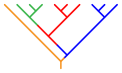
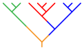
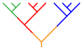
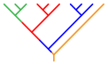
$S_{0}^{\prime}=Y\backslash(S_{0}/S_{1}/S_{2})$ $S_{1}^{\prime}=S_{0}/Y\backslash(S_{1}/S_{2})$ $S_{2}^{\prime}=(S_{0}/S_{1})/Y\backslash S_{2}$ $S_{3}^{\prime}=(S_{0}/S_{1}/S_{2})/Y$

Figure 5. The binary trees $S_{k}^{\prime}$ for $0\leq k\leq 3$ obtained from the binary tree $S$ of Figure 3 in the proof of Proposition 12.

See Figure 5. For the extreme values of $k$, we have $S_{0}^{\prime}=Y\backslash S$ and $S_{\ell(S)}^{\prime}=S/Y$. Moreover, any indecomposable Tamari interval $(S^{\prime},T^{\prime})$ with $n(S^{\prime})=n(T^{\prime})>1$ is obtained in a single way by this procedure. Since $\ell(S_{k}^{\prime})=k$, ${n(S^{\prime})=n(S)+1}$, $\operatorname{des}(S^{\prime})=\operatorname{des}(S)+1$ when $k\leq\ell(S)$ while ${\operatorname{des}(S_{\ell(S)+1}^{\prime})=\operatorname{des}(S)}$, and $\operatorname{asc}(T^{\prime})=\operatorname{asc}(T)$, we obtain

(2) $$A^{\circ}_{u}=t\Big{(}1+z\frac{uA_{u}-A_{1}}{u-1}+uA_{u}\Big{)}.$$

Combining Equations 1 and 2, we obtain

$$A_{u}=t\Big{(}1+z\frac{u^{2}A_{u}-A_{1}}{u-1}+uA_{u}\Big{)}\big{(}1+uzA_{u}\big{)},$$

which rewrites as

$$(u-1)A_{u}=t\big{(}u-1+u(u+z-1)A_{u}-zA_{1}\big{)}\big{(}1+uzA_{u}\big{)}.\qed$$

We are now ready to derive our functional equation on $A$ using the quadratic method [GJ04].

Proposition 13.

The generating function $A=A(t,z)$ is a root of the polynomial $P(t,z,X)$ of $\mathbb{Q}[t,z,X]$ given by

$$t^{3}z^{6}X^{4}$$

$${}+t^{2}z^{4}(tz^{2}+6tz-3t+3)X^{3}$$

$${}+tz^{2}(6t^{2}z^{3}+9t^{2}z^{2}-12t^{2}z+2tz^{2}+3t^{2}-6tz+21t+3)X^{2}$$

$${}+(12t^{3}z^{4}-4t^{3}z^{3}-9t^{3}z^{2}-10t^{2}z^{3}+6t^{3}z+26t^{2}z^{2}-t^{3}+6t^{2}z+tz^{2}+3t^{2}-12tz-3t+1)X$$

$${}+t(8t^{2}z^{3}-12t^{2}z^{2}+6t^{2}z-tz^{2}-t^{2}+10tz+2t-1).$$

Proof.

We simply apply the quadratic method [GJ04]. The quadratic equation of Proposition 12 can be rewritten as $\alpha A_{u}^{2}+\beta A_{u}+\gamma=0,$ where

$$\alpha=tu^{2}z(u+z-1),\quad\beta=tu(u+z-1)+tuz(u-1)-tuz^{2}A_{1}-u+1,\quad\gamma=t(u-1)-tzA_{1}.$$

The discriminant $\Delta\mbox{\,\raisebox{0.86108pt}{\scriptsize$\mathrm{:}$}$=$\,}\beta^{2}-4\alpha\gamma$ must have multiple roots, which implies that its own discriminant in $u$ vanishes. Removing clearly non-vanishing factors, this leads to the equation of the statement. Note that $\Delta$ having only degree $4$ in $v$, the formula for the discriminant could be worked out by hand. ∎

Remark 14.

When specialized at $z=0$, Proposition 13 shows that $A(t,0)$ is a root of the polynomial

$$P(t,0,X)=-(t-1)^{3}X-t(t-1)^{2}$$

which recovers the fact that $A(t,0)=t/(1-t)=t+t^{2}+t^{3}+\cdots$.

Remark 15.

When specialized at $z=1$, Proposition 13 shows that $A(t,1)$ is a root of the polynomial

$$P(t,1,X)=t^{3}X^{4}+t^{2}(4t+3)X^{3}+t(6t^{2}+17t+3)X^{2}+(4t^{3}+25t^{2}-14t+1)X+t^{3}+11t^{2}-t.$$

This is the classical functional equation for the generating function of Tamari intervals (see e.g.  [Cha07, Eq. (5)]). The curve defined by $P(t,1,X)$ has genus zero and admits the rational parametrization

(3) $$t=\frac{s}{(s+1)^{4}},\quad X=s-s^{2}-s^{3}.$$

As a consequence, the unique root $A=A(t,1)=t+3t^{2}+13t^{3}+68t^{4}+399t^{5}+2530t^{6}+\cdots$ in $\mathbb{Q}[[t]]$ of the polynomial $P(t,1,X)$ can be written as

(4) $$A=S-S^{2}-S^{3},$$

where $S=t+4t^{2}+22t^{3}+140t^{4}+\cdots$ is the unique solution in $\mathbb{Q}[[t]]$ of

$$t=\frac{S}{(S+1)^{4}}.$$

From this equation, the coefficients of $S$, $S^{2}$ and $S^{3}$ can be computed via Lagrange inversion. More precisely, for $r\geq 1$, Lagrange inversion gives

$$[t^{n}]S^{r}=\frac{1}{n}[s^{n-1}]\,rs^{r-1}\phi(s)^{n}=\frac{r}{n}[s^{n-r}]\phi(s)^{n},$$

where $\phi(s)\mbox{\,\raisebox{0.86108pt}{\scriptsize$\mathrm{:}$}$=$\,}(s+1)^{4}$. Since

$$[s^{a}]\phi(s)^{n}=[s^{a}](s+1)^{4n}=\binom{4n}{a},$$

we obtain that, for $r\in\{1,2,3\}$,

$$[t^{n}]S^{r}=\frac{r}{n}[s^{n-r}]\phi(s)^{n}=\frac{r}{n}\binom{4n}{n-r}.$$

Hence, Equation 4 implies that

$$[t^{n}]A=[t^{n}]S-[t^{n}]S^{2}-[t^{n}]S^{3}$$

is given by

$$\frac{1}{n}\left(\binom{4n}{n-1}-2\binom{4n}{n-2}-3\binom{4n}{n-3}\right)=\frac{2}{(3n+1)(3n+2)}\binom{4n+1}{n+1},$$

as proved in [Cha07, Thm. 2.1].

3. Lagrange inversion and binomial identity

We now present our first proof of Theorems 1 and 2. For Theorem 1, we reparametrize the polynomial equation of Proposition 13 and extract the coefficients of $A(t,z)$ by Lagrange inversion (Section 3.1). We then prove that Theorem 1 implies Theorem 2 by using a simple binomial identity (Section 3.2).

3.1. Theorem 1 by Lagrange inversion

We will now mimic the approach in Remark 15, and extract the coefficients of $A(t,z)$ to obtain Theorem 1. The starting point is that the curve in $t,X$ defined by the polynomial $P(t,z,X)\in\mathbb{Q}(z)[t,X]$ from Proposition 13 still has genus zero and admits the following rational parametrization:

(5) $$t=\frac{s}{(s+1)(sz+1)^{3}},\quad X=s-zs^{2}-zs^{3},$$

which lifts the parametrization (3). As a consequence, the unique root $A$ in $\mathbb{Q}[[t,z]]$ of the polynomial $P(t,z,X)$ can be written

(6) $$A=S-zS^{2}-zS^{3},$$

where $S=t+\left(3z+1\right)t^{2}+\left(12z^{2}+9z+1\right)t^{3}+\cdots$ is the unique solution in $\mathbb{Q}[z][[t]]$ of

(7) $$t=\frac{S}{(S+1)(Sz+1)^{3}}.$$

There exist infinitely many rational parametrizations of $P$, but the one in Equation 5 has a double advantage: on the one hand, Equation 7 is under a form amenable to Lagrange inversion, and therefore allows to express the coefficient of $z^{k}t^{n}$ in $S$ and in its powers; on the other hand, the simple form of Equation 6 allows to easily extract the coefficient of $t^{n}z^{k}$ in $A$ as a sum of similar coefficients of $S$, $S^{2}$ and $S^{3}$. Putting together Equations 6 and 7 enables us to express the coefficient of $t^{n}z^{k}$ in $A$ as a binomial sum. Let us give a few more details.

For $r\geq 1$ Lagrange inversion gives

$$[t^{n}z^{k}]S^{r}=\frac{1}{n}[s^{n-1}z^{k}]rs^{r-1}\phi(s)^{n}=\frac{r}{n}[s^{n-r}z^{k}]\phi(s)^{n},$$

where $\phi(s)\mbox{\,\raisebox{0.86108pt}{\scriptsize$\mathrm{:}$}$=$\,}(s+1)(sz+1)^{3}$. We have that

$$[s^{a}]\phi(s)^{n}=[s^{a}](s+1)^{n}(sz+1)^{3n}=\sum_{i+j=a}\binom{n}{i}\binom{3n}{j}z^{j},$$

and therefore

$$[s^{a}z^{k}]\phi(s)^{n}=\binom{n}{a-k}\binom{3n}{k}.$$

It follows that, for $r\in\{1,2,3\}$,

$$[t^{n}z^{k}]S^{r}=\frac{r}{n}[s^{n-r}z^{k}]\phi(s)^{n}=\frac{r}{n}\binom{n}{n-r-k}\binom{3n}{k}=\frac{r}{n}\binom{n}{k+r}\binom{3n}{k},$$

Hence, Equation 6 implies that

$$a_{n,k}=[t^{n}z^{k}]A=[t^{n}z^{k}]S-[t^{n}z^{k-1}]S^{2}-[t^{n}z^{k-1}]S^{3}$$

is given by

$$\frac{1}{n}\left(\binom{n}{k+1}\binom{3n}{k}-2\binom{n}{k+1}\binom{3n}{k-1}-3\binom{n}{k+2}\binom{3n}{k-1}\right)=\frac{2}{n(n+1)}\binom{3n}{k}\binom{n+1}{k+2},$$

which proves Theorem 1.

3.2. Theorem 2 by a binomial identity

We now simply derive Theorem 2 from Theorem 1, which amounts to checking the following binomial identity.

Proposition 16.

For any $n,k\in\mathbb{N}$,

$$\sum_{\ell=k}^{n-1}\frac{2}{n(n+1)}\binom{n+1}{\ell+2}\binom{3n}{\ell}\binom{\ell}{k}=\frac{2}{(3n+1)(3n+2)}\binom{n-1}{k}\binom{4n+1-k}{n+1}.$$

We shall actually prove the following generalization.

Proposition 17.

For any $n,k,r\in\mathbb{N}$,

$$\sum_{\ell=k}^{n-1}\binom{n+1}{\ell+2}\binom{r}{\ell}\binom{\ell}{k}=\frac{n(n+1)}{(r+1)(r+2)}\binom{n-1}{k}\binom{r+n+1-k}{n+1}.$$

Proof.

Using the identity

$$\binom{r}{\ell}\binom{\ell}{k}=\binom{r}{k}\binom{r-k}{r-\ell}$$

this amounts to showing that

$$\binom{r}{k}\sum_{\ell\geq 0}\binom{n+1}{\ell+2}\binom{r-k}{r-\ell}=\frac{n(n+1)}{(r+1)(r+2)}\binom{n-1}{k}\binom{r+n+1-k}{n+1}.$$

This is in turn equivalent to

$$\sum_{\ell\geq 0}\binom{n+1}{\ell+2}\binom{r-k}{r-\ell}=\binom{r+n+1-k}{r+2},$$

which is a particular case of the classical Chu–Vandermonde identity. ∎

4. Creative telescoping

In Section 3, we benefited from two interesting coincidences to derive simple proofs of Theorems 1 and 2. We now present a more robust method based on recurrence relations obtained by creative telescoping, and prove that Theorem 1 (Section 4.1), Theorem 2 (Section 4.2), and Proposition 17 (Section 4.3) can all be systematically obtained by this method.

4.1. Theorem 1 by creative telescoping

After guessing the binomial expression for $a_{n,k}$ stated in Theorem 1, proving the theorem amounts to a combination of well established algorithms in computer algebra.

Proposition 13 expresses that the bivariate series $A$ of $\mathbb{Q}[[t,z]]$ is algebraic: the infinite family of its powers $A^{i}$ spans a finite-dimensional vector space over $\mathbb{Q}(t,z)$, whose dimension $d=4$ is the degree in $X$ of the polynomial $P(t,z,X)$ satisfying $P(t,z,A(t,z))=0$ given by the proposition.

It is well known [Sta80, Lip89] that an algebraic formal power series like $A$ is D-finite with respect to $t$ and $z$, that is, the infinite family of the derivatives $\partial^{i+j}A/\partial t^{i}\partial z^{j}$ spans a finite-dimensional vector space over $\mathbb{Q}(t,z)$. Indeed, taking a derivative with respect to $t$ yields a relation

$$P_{t}(t,z,A(t,z))+P_{X}(t,z,A(t,z))\frac{\partial A(t,z)}{\partial t}=0.$$

So $\partial A/\partial t$ is a rational function of $A$, which can therefore be expressed in the form

$$\frac{\partial A(t,z)}{\partial t}=Q^{(1)}(t,z,A(t,z))$$

for a polynomial $Q^{(1)}(t,z,X)$ in $\mathbb{Q}(t,z)[X]$ of degree at most $d-1$ in $X$. Taking a further derivative yields

$$\frac{\partial^{2}A(t,z)}{\partial t^{2}} =Q_{t}^{(1)}(t,z,A(t,z))+Q_{X}^{(1)}(t,z,A(t,z))\frac{\partial A(t,z)}{\partial t}$$

$$=Q_{t}^{(1)}(t,z,A(t,z))+Q_{X}^{(1)}(t,z,A(t,z))Q^{(1)}(t,z,A(t,z))=Q^{(2)}(t,z,A(t,z))$$

for another polynomial $Q^{(2)}(t,z,X)$ in $\mathbb{Q}(t,z)[X]$ of degree at most $d-1$ in $X$. Continuing in this way provides a family of polynomials of degree at most $d-1$ in $X$,

$$Q^{(0)}=X,Q^{(1)},\dots,Q^{(d)}.$$

These $d+1$ polynomials have a linear dependency over $\mathbb{Q}(t,z)$, which expresses a nontrivial linear differential equation satisfied by $X(t,z)$, of the form

(8) $$p_{d}(t,z)\frac{\partial^{d}X(t,z)}{\partial t^{d}}+\dots+p_{0}(t,z)X(t,z)=0$$

for polynomials $p_{i}(t,z)\in\mathbb{Q}[t,z]$. A slight variant introduces $Q^{(-1)}=1$ and searches for a dependency between $Q^{(-1)},\dots,Q^{(d-1)}$, which makes it possible to obtain a nonhomogeneous relation, that is, with a polynomial $q(t,z)\in\mathbb{Q}[t,z]$ in place of $0$ as the right-hand side of Equation 8.

Such a nonhomogeneous relation is easily computed by using the command algeqtodiffeq of the package gfun for Maple, resulting in an equation consisting of $135$ monomials, of the form

(9) $$(27t^{2}z^{4}-108t^{2}z^{3}+\dotsb)(6t^{2}z^{5}-33t^{2}z^{4}+\dotsb)t^{3}\frac{\partial^{3}X}{\partial t^{3}}+3(216t^{4}z^{9}-2052t^{4}z^{8}+\dotsb)t^{2}\frac{\partial^{2}X}{\partial t^{2}}\\ +6(60t^{4}z^{9}-570t^{4}z^{8}+\dotsb)t\frac{\partial X}{\partial t}+(12t^{3}z^{7}+6t^{3}z^{6}+\dotsb)X=12t(2t^{2}z^{7}-23t^{2}z^{6}+\dotsb).$$

Next, we know that the series solution $A$ is more precisely an element of $\mathbb{Q}[z][[t]]$, and we write it in the form $A=\sum_{n\geq 0}a_{n}(z)t^{n}$. For a general series of this type, extracting the coefficient of $t^{n}$ from Equation 8 and arranging terms yields a nonhomogeneous linear recurrence relation of some order $r$ between finitely many shifts $a_{n+i}(z)$ with $i\in\mathbb{Z}$, valid for all $n$ large enough, say ${n\geq n_{0}\geq 0}$, as well as some linear dependence relations between the initial values, $a_{0}(z)$ to $a_{n_{0}+r-1}(z)$. Applying this procedure to Equation 9, this time by using gfun’s command diffeqtorec, returns

(10) $$9(n+5)(3n+14)(3n+13)(2z-3)a_{n+4}(z)+(44550+\dots-78n^{3}z^{4})a_{n+3}(z)\\ +(z-1)(2n+5)(4536+\dots+4n^{2}z^{6})a_{n+2}(z)+3(z-1)^{4}(900+\dots-26n^{3}z^{4})a_{n+1}(z)\\ +9n(2z-3)(z-1)^{8}(3n+2)(3n+1)a_{n}(z)=0,$$

where we ensured that all coefficients are polynomial expressions in $\mathbb{Q}[n,z]$. The mere calculation proves that this recurrence is valid for all $n\geq 0$, and because the coefficient of $a_{n+4}(z)$ does not vanish for any nonnegative value of $n$, the sequence $(a_{n}(z))_{n\geq 0}$ is uniquely defined as a solution of Equation 10 by its initial values $a_{0}(z),\dots,a_{3}(z)$.

At this point, proving Theorem 1 reduces to:

1. proving that the sequence of polynomials

   $$\tilde{a}_{n}(z)\mbox{\,\raisebox{0.86108pt}{\scriptsize$\mathrm{:}$}$=$\,}\sum_{k=0}^{n-1}\tilde{a}_{n,k},\qquad\text{where}\qquad\tilde{a}_{n,k}\mbox{\,\raisebox{0.86108pt}{\scriptsize$\mathrm{:}$}$=$\,}\frac{2}{n(n+1)}\binom{n+1}{k+2}\binom{3n}{k}z^{k},$$

   satisfies the same recurrence relation (10) as the sequence $(a_{n}(z))_{n\geq 0}$,

2. checking $\tilde{a}_{i}(z)=a_{i}(z)$ for $0\leq i\leq 3$.

The second point is done by easy calculations. For the first point, we appeal to the method of creative telescoping [Zei91, Zei90, PWZ96], whose goal is to obtain a recurrence of the specific form,

(11) $$\sum_{i=0}^{\tilde{r}}\eta_{i}(n)\tilde{a}_{n+i,k}=R(n,k+1)\tilde{a}_{n,k+1}-R(n,k)\tilde{a}_{n,k},$$

for some $\tilde{r}\in\mathbb{N}$, rational functions $\eta_{i}(n)\in\mathbb{Q}(z,n)$, $0\leq i\leq\tilde{r}$, and $R(n,k)\in\mathbb{Q}(z,n,k)$ (we keep the parameter $z$ implicit in the notation). The motivation is that, after verifying certain conditions of nondivergence, summing Equation 11 over $k\in\mathbb{Z}$, which in fact involves finite sums only, and observing that the right-hand side telescopes to zero, results in a homogeneous recurrence for the $\tilde{a}_{n}(z)$. The popular variant of the original algorithm rewrites Equation 11 into

(12) $$\sum_{i=0}^{\tilde{r}}\eta_{i}(n)\left[\frac{\tilde{a}_{n+i,k}}{\tilde{a}_{n,k}}\right]=R(n,k+1)\left[\frac{\tilde{a}_{n,k+1}}{\tilde{a}_{n,k}}\right]-R(n,k)$$

and analyzes the zeros and poles of the (known) bracketed rational function in the right-hand side to predict a universal denominator bound $B(n,k)$ for the unknown $R$. After writing $R(n,k)=P(n,k)/B(n,k)$, Equation 12 is transformed into a similar-looking recurrence for the polynomial $P(n,k)$. After deriving a bound on the degree of $P$ with respect to $k$, the method then proceeds by undetermined coefficients and linear algebra over $\mathbb{Q}(n)$ to obtain the coefficients with respect to $k$ of $P$ and the $\eta_{i}$. The latter form a (possibly empty) affine space. Because a successful $\tilde{r}$ is not known beforehand, the method tests increasing values of $\tilde{r}$ in $\mathbb{N}$, without proven termination, but if it terminates, it returns with the minimal order $\tilde{r}$ such that Equation 11 is possible.

Zeilberger’s so-called “fast algorithm”, which has just been described and is implemented by Maple’s command SumTools:-Hypergeometric:-Zeilberger, tests increasing orders up to the order $\tilde{r}=2$, resulting in:

$$\eta_{2}(n)=3(3n+7)(n+3)(3n+8)(n^{2}z^{2}-6n^{2}z+2nz^{2}-27n^{2}-12nz-54n-30),\\ \eta_{1}(n)=-(2n+3)(2n^{4}z^{5}-21n^{4}z^{4}+12n^{3}z^{5}+108n^{4}z^{3}-126n^{3}z^{4}+22n^{2}z^{5}-378n^{4}z^{2}\\ {}+648n^{3}z^{3}-231n^{2}z^{4}+12nz^{5}-3078n^{4}z-2268n^{3}z^{2}+1188n^{2}z^{3}-126nz^{4}\\ -729n^{4}-18468n^{3}z-4188n^{2}z^{2}+648nz^{3}-4374n^{3}-39078n^{2}z-2358nz^{2}\\ -10449n^{2}-34128nz-11664n-10080z-5040),\\ \eta_{0}(n)=3n(z-1)^{4}(3n+2)(3n+1)\\ \times(n^{2}z^{2}-6n^{2}z+4nz^{2}-27n^{2}-24nz+3z^{2}-108n-18z-111)$$

and in a rational function $R$:

1. whose numerator has total degree $18$ in $n$ and $k$, consists of $402$ terms in expanded form, and involves integers up to $10$ decimal digits,

2. whose denominator is the product of the $k-\alpha$ over $\alpha$ in

   $$Z=\{n,n+1,3n+1,3n+2,3n+3,3n+4,3n+5,3n+6\}.$$

Note that by replacing various terms like $\binom{n+i}{k+j}$ and $\binom{3n+i}{k+j}$ by suitable rational multiples of $\binom{n}{k}$ and $\binom{3n}{k}$ and by normalizing rational functions, we verify that Equation 11 holds for all $n\geq 0$ and all $k$ such that $k\not\in Z$ and $k+1\not\in Z$.

Observe that using Equation 11 to produce all of $\tilde{a}_{n}(z)$, …, $\tilde{a}_{n+\tilde{r}}(z)$ requires summing it up to at least $k=n+\tilde{r}-1=n+1$, whereas its right-hand side has pole (at least syntactically) at $n-1$, $n$, $n+1$, $3n$, and at a few more values beyond. This prevents us from summing as wanted. A solution to circumvent this issue is rarely properly exposed in the literature. A rare exception is the technical report [APS04], where the authors modify a priori diverging expressions by shifting arguments in binomial expressions so as to make denominators disappear. Here, we use a technique that was called sound creative telescoping in [CMSPT14] (see also [KP11, p. 99] for the simpler univariate situation, and [Har15, Sect. 4] for an alternative rigorous limiting argument). Sound creative telescoping consists in summing Equation 11 over $k$ from $-1$ to $n-2$ and adding missing terms to both sides, thus obtaining

$$\sum_{i=0}^{2}\eta_{i}(n)\tilde{a}_{n+i}(z)=R(n,n-1)\tilde{a}_{n,n-1}-R(n,-1)\tilde{a}_{n,-1}+\sum_{i=0}^{2}\eta_{i}(n)\sum_{k=n-1}^{n+i}\tilde{a}_{n+i,k}.$$

Simplifying the right-hand side by the formula $\binom{n}{-1}=0$ and by replacing various $\binom{n+i}{k+j}$ by suitable rational multiples of $\binom{n}{k}$, then taking a normal form, shows that the right-hand side is in fact $0$:

(13) $$\sum_{i=0}^{2}\eta_{i}(n)\tilde{a}_{n+i}(z)=0.$$

Because $\eta_{2}(n)$ does not vanish for any nonnegative value of $n$, $\tilde{a}_{n+3}(z)$ and $\tilde{a}_{n+4}(z)$ can be uniquely expressed as linear combinations of $\tilde{a}_{n}(z)$, $\tilde{a}_{n+1}(z)$, and $\tilde{a}_{n+2}(z)$ with well-defined rational function coefficients in $\mathbb{Q}(z,n)$, thus providing identities valid for all $n\geq 0$. Upon replacing the $a_{n}(z)$ with those expressions for $\tilde{a}_{n}(z)$ in the left-hand side of Equation 10 and simplifying, we finally get that the sequence $(\tilde{a}_{n}(z))_{n\geq 0}$ satisfies the same recurrence relation (10) as $(a_{n}(z))_{n\geq 0}$.

Remark 18.

Note the drop by one from the algebraic degree $d=4$ of $X$ in $P$ to the differential order in Equation 9: taking a derivative of Equation 9 and recombining would result in a differential equation of order $d$. By contrast, the fact that the order of the recurrence (10) and the number of defining initial values both happen to match the algebraic degree $d=4$ is a coincidence: the recurrence order could be larger in general.

Remark 19.

In general, the method need not lead to a recurrence (13) whose solutions should all also satisfy Equation 10. In such situations, one should first determine a recurrence valid for the difference $\tilde{a}_{n}(z)-a_{n}(z)$, which algorithmically is obtained as a recurrence valid for all linear combinations $\lambda\tilde{a}_{n}(z)+\mu a_{n}(z)$, and can be viewed as a noncommutative least common multiple of the recurrences. The theory originates in Ore’s works in the 1930s, see [BP96] for a modern treatment. Concrete calculations can be done by using gfun’s command ‘rec+rec‘.

Remark 20.

If the summand $\tilde{a}_{n,k}$ did not exhibit a denominator $n(n+1)$, another method would apply, namely the theory of binomial sums in the sense of [BLS17]. In certain instances, it has been possible to modify the expression of $\tilde{a}_{n,k}$, by playing around with shifts in the binomials to get rid of the denominator; in the present case however, we were unable to find such a reformulation.

4.2. Theorem 2 by creative telescoping

We now observe that the exact same method used in Section 4.1 can be exploited to prove Theorem 2. For this, we first obtain a polynomial equation on the generating function $B(t,z)\mbox{\,\raisebox{0.86108pt}{\scriptsize$\mathrm{:}$}$=$\,}\sum b_{n,k}t^{n}z^{k}$ from Proposition 13 and the following immediate observation.

Lemma 21.

We have $A(t,z+1)=B(t,z)$.

Proof.

The coefficient of $t^{n}$ in $A(t,z+1)$ is given by

$$[t^{n}]A(t,z+1) =\sum_{\ell=0}^{n-1}a_{n,\ell}(z+1)^{\ell}=\sum_{\ell=0}^{n-1}a_{n,\ell}\sum_{k=0}^{\ell}\binom{\ell}{k}z^{k}$$

$$=\sum_{k=0}^{n-1}\sum_{\ell=k}^{n-1}\binom{\ell}{k}a_{n,\ell}z^{k}=\sum_{k=0}^{n-1}b_{n,k}z^{k}=[t^{n}]B(t,z).\qed$$

Substituting $z$ with $z+1$ in Proposition 13, we thus obtain the following polynomial equation on $B$, given in terms of the polynomial $P(t,z,X)$ provided by Proposition 12.

Corollary 22.

The generating function $B=B(t,z)$ is a root of the polynomial $P(t,z+1,X)$ of $\mathbb{Q}[t,z,X]$, which is equal to

$$t^{3}(z+1)^{6}X^{4}$$

$${}+t^{2}(z+1)^{4}(tz^{2}+8tz+4t+3)X^{3}$$

$${}+t(z+1)^{2}(6t^{2}z^{3}+27t^{2}z^{2}+24t^{2}z+2tz^{2}+6t^{2}-2tz+17t+3)X^{2}$$

$${}+(12t^{3}z^{4}+44t^{3}z^{3}+51t^{3}z^{2}-10t^{2}z^{3}+24t^{3}z-4t^{2}z^{2}+4t^{3}+28t^{2}z+tz^{2}+25t^{2}-10tz-14t+1)X$$

$${}+t(8t^{2}z^{3}+12t^{2}z^{2}+6t^{2}z-tz^{2}+t^{2}+8tz+11t-1).$$

Before going further, we now quickly transpose Remarks 14 and 15 in terms of specializations in $B$.

Remark 23.

When specialized at $z=-1$, Corollary 22 shows that $B(t,1)$ is a root of the polynomial

$$P(t,0,X)=-(t-1)^{3}X-t(t-1)^{2}$$

hence $B(t,-1)=\bar{B}(t,-1)=t/(1-t)$. This shows that

$$\sum_{0\leq k<n}\frac{2(-1)^{k}}{(3n+1)(3n+2)}\binom{n-1}{k}\binom{4n+1-k}{n+1}=1$$

for any $n\in\mathbb{N}$. This can also be directly derived from Euler’s relation on the cellular diagonal of the associahedron (seen as a polytopal decomposition of the associahedron).

Remark 24.

When specialized at $z=0$, Corollary 22 shows that $B(t,0)$ is the root of the polynomial

$$P(t,1,X)=t^{3}X^{4}+t^{2}(4t+3)X^{3}+t(6t^{2}+17t+3)X^{2}+(4t^{3}+25t^{2}-14t+1)X+t^{3}+11t^{2}-t.$$

and we obtain by reparametrization and Lagrange inversion the formula

$$\frac{2}{(3n+1)(3n+2)}\binom{4n+1}{n+1}$$

proved in [Cha07] as explained in Remark 15.

Remark 25.

It is possible to express $A(t,z+1)=B(t,z)=t+\left(2z+3\right)t^{2}+\left(6z^{2}+18z+13\right)t^{3}+\cdots$ from Corollary 22 in terms of “simple” algebraic functions. More precisely, let $p$ and $q$ be the rational functions

$$p=\frac{3z^{2}}{8\left(z+1\right)^{2}},\quad q=\frac{t\,z^{3}-8}{8t\left(z+1\right)^{3}},$$

then let $a,b$ and $c$ be the algebraic functions

$$a=12t\left(9t\,z^{2}+9+\sqrt{81t^{2}z^{4}-12t\,z^{3}+18t\,z^{2}-576tz-768t+81}\right),$$

$$b=\frac{1}{\left(z+1\right)^{2}}\cdot\left(\frac{\sqrt[3]{a}}{6t}+\frac{2z+8}{\sqrt[3]{a}}-\frac{z^{2}}{8}\right),\quad c=\frac{\sqrt{b+p}}{2}-\frac{\sqrt{p-b-\frac{2q}{\sqrt{b+p}}}}{2}-\frac{z+4}{4z+4}.$$

Then,

(14) $$B=c-\left(z+1\right)c^{2}-\left(z+1\right)c^{3}.$$

One can prove this expression as follows. First, by (7), $c=S(z+1,t)=t+\left(3z+4\right)\,t^{2}+\left(12z^{2}+33z+22\right)\,t^{3}+\cdots$ is the unique root in $\mathbb{Q}[z][[t]]$ of

(15) $$t=\frac{c}{(c+1)(cz+c+1)^{3}},$$

and Equation 6 implies Equation 14. Equation 15 can be solved using the Ferrari–Cardano formulas [Kur88, Chap. 9]. First, $\tilde{c}=c-(z+4)/(4z+4)$ is seen to satisfy the equation $\tilde{c}^{4}-p\tilde{c}^{2}+q\tilde{c}+r=0$ with $p,q$ defined as above and $r=\frac{z+4}{4t\left(z+1\right)^{4}}-\frac{3z^{4}}{256\left(z+1\right)^{4}}$. This equation can be solved using Ferrari’s formulas, by reducing to the third-order equation $Y^{3}+pY^{2}-4rY-(4pr+q^{2})=0$, itself solved using the Cardano formulas, and finally to the second-order equation $\tilde{c}^{2}\pm\sqrt{Y+p}\cdot(\tilde{c}-q/(2(Y+p)))+Y/2=0$. We omit the details, leading to the expressions of $a,b$ and $c$ above.

At this point, a direct proof of Theorem 2 based on creative telescoping parallels the proof in Section 4.1: as $z$ plays no role beyond that of a parameter in the constant field for the proof there, changing it to $z+1$ has no impact beyond changing the coefficients in $\mathbb{Q}(z)$ of the expressions involved. For example, the reader will compare the differential equation (9) satisfied by $A(t,z)$ with its equivalent for $B(t,z)$:

$$(27t^{2}z^{4}-4tz^{3}+\dotsb)(6t^{2}z^{5}-3t^{2}z^{4}+\dotsb)t^{3}\frac{\partial^{3}X}{\partial t^{3}}+3(216t^{4}z^{9}-108t^{4}z^{8}+\dotsb)t^{2}\frac{\partial^{2}X}{\partial t^{2}}\\ +6(60t^{4}z^{9}-30t^{4}z^{8}+\dotsb)t\frac{\partial X}{\partial t}+(12t^{3}z^{7}+90t^{3}z^{6}+\dotsb)X=12t(2t^{2}z^{7}-9t^{2}z^{6}+\dotsb),$$

and the recurrence relation (10) for the coefficients $a_{n}(z)$ of $A(t,z)$ with its equivalent for the coefficients $b_{n}(z)$ of $B(t,z)$,

$$9(n+5)(3n+14)(3n+13)(2z-1)b_{n+4}(z)+(42840+\dots-78n^{3}z^{4})b_{n+3}(z)\\ +z(2n+5)(25344+\dots+4n^{2}z^{6})b_{n+2}(z)+3z^{4}(360+\dots-26n^{3}z^{4})b_{n+1}(z)\\ +9n(2z-1)z^{8}(3n+2)(3n+1)b_{n}(z)=0.$$

The proof also introduces the sequence of polynomials

$$\tilde{b}_{n}(z)\mbox{\,\raisebox{0.86108pt}{\scriptsize$\mathrm{:}$}$=$\,}\sum_{k=0}^{n-1}\tilde{b}_{n,k},\qquad\text{where}\qquad\tilde{b}_{n,k}\mbox{\,\raisebox{0.86108pt}{\scriptsize$\mathrm{:}$}$=$\,}\frac{2}{(3n+1)(3n+2)}\binom{n-1}{k}\binom{4n+1-k}{n+1}z^{k},$$

to show that it satisfies the same recurrence relation as the sequence $(b_{n}(z))_{n\geq 0}$. Again, the calculation is the same as for the sum $\tilde{a}_{n}(z)$, and we obtain coefficients $\eta_{0}$, …, $\eta_{2}$ of a recurrence that are the result of applying a backward shift with respect to $z$ to the polynomials obtained in the previous section, e.g. the new $\eta_{2}$ is

$$3(3n+7)(n+3)(3n+8)(n^{2}z^{2}-4n^{2}z+2nz^{2}-32n^{2}-8nz-64n-30).$$

The noncomputational arguments of the proof are unchanged.

4.3. Proposition 16 and Proposition 17 by creative telescoping

We finally provide an alternative proof of Proposition 16 and Proposition 17 by using recurrence relations. We focus on the latter. Note that the identity to be proven is the tautology $0=0$ if $k\geq n$, so we focus on the case $k<n$.

Define

$$s_{n,k,r,\ell}\mbox{\,\raisebox{0.86108pt}{\scriptsize$\mathrm{:}$}$=$\,}\binom{n+1}{\ell+2}\binom{r}{\ell}\binom{\ell}{k}\qquad\text{and}\qquad S_{n,k,r}\mbox{\,\raisebox{0.86108pt}{\scriptsize$\mathrm{:}$}$=$\,}\sum_{\ell=k}^{n-1}s_{n,k,r,\ell}.$$

Using Maple’s command SumTools:-Hypergeometric:-Zeilberger(s, k, l, sk), where s denotes a variable containing a Maple encoding of $s_{n,k,r,\ell}$ and sk denotes a forward-shift operator to be used in the output, an immediate calculation returns an encoding of the relation:

$$(k+1)(n+r+1-k)s_{n,k+1,r,\ell}+(r-k)(n-k-1)s_{n,k,r,\ell}=(\ell+3)(k-\ell-1)s_{n,k,r,\ell+1}-(\ell+2)(k-\ell)s_{n,k,r,\ell}.$$

Because the summand $s_{n,k,r,\ell}$ is well defined at any $\ell\in\mathbb{Z}$ and zero out of the (finite) summation range, summing the previous relation over $\ell\in\mathbb{Z}$ results in

$$(k+1)(n+r+1-k)S_{n,k+1,r}+(r-k)(n-k-1)S_{n,k,r}=0.$$

Because we assumed $k<n$, the coefficient of $S_{n,k+1,r}$ is nonzero. It is immediate to check that the right-hand side of the identity to be proven satisfies the same recurrence, so the quotient of the sum and the right-hand side is a function of $(n,r)$. Verifying that this ratio is $1$ reduces to checking the case $k=n-1$ (forcing $\ell=n-1$ in the sum), that is,

$$\binom{n+1}{n+1}\binom{r}{n-1}\binom{n-1}{n-1}=\frac{n(n+1)}{(r+1)(r+2)}\binom{n-1}{n-1}\binom{r+2}{n+1},$$

which holds as is seen by rewriting into factorials.

Remark 26.

Using the package Mgfun, specifically its command creative_telescoping, in the form

creative_telescoping(s, [n::shift, k::shift, r::shift], [l::shift])

where s stands for a Maple variable containing the summand, readily results in a system of equations of the form

$$\sum_{0\leq h,i,j\leq\rho}\eta_{h,i,j}(n,k)s_{n+h,k+i,r+j,\ell}=R(n,k,\ell+1)s_{n,k,\ell+1}-R(n,k)s_{n,k,\ell},$$

thus generalizing the pattern (11). The output revealed the existence of a first-order recurrence with respect to $k$ for the sum, which guided us towards the proof given above, using plain Maple. Working with $n$, which seems to be a more dominant parameter, instead of $k$, leads to more difficult calculations.

Remark 27.

Proposition 16 can be viewed as the case $r=3n$ in Proposition 17. It turns out that the computational proof with SumTools:-Hypergeometric:-Zeilberger goes along exactly the same lines, with occurrences of $3n$ replacing $r$ and of $4n$ replacing $n+r$. The computation with creative_telescoping makes a few more changes, principally because it has to accommodate an additional independent equation to reflect the dependency in $r$.

5. Solving a holonomic recurrence system

Section 4.1 showed how the polynomial $P$ from Proposition 13 can be translated into a differential equation with respect to $t$ on the series $A(t,z)$, which can in turn be translated into a recurrence equation with respect to $n$ on the coefficients $[t^{n}]A(t,z)$. In this section, we proceed similarly to derive a system of recurrence equations with respect to $n$ and $k$ on the coefficients $[t^{n}z^{k}]A(t,z)$, before simplifying and solving the system so as to identify the sequence $(a_{n,k})_{(n,k)\in\mathbb{Z}^{2}}$ given in Theorem 1 as its solution, thus providing a third proof of Theorem 1. We also comment on our unsuccess to deal with Theorem 2 by the same approach.

Variants of the method that was used to obtain Equation 9 from the polynomial $P$ exist to compute differential equations with respect to $z$ instead of $t$, and even a complete set of equations between cross derivatives. In particular, if P denotes a variable containing the polynomial $P(t,z,X)$ in the (Maple) variables t, z, X, using Mgfun’s command dfinite_expr_to_sys in the form

dfinite_expr_to_sys(RootOf(P, X), A(t::diff, z::diff))

results in a system of three homogeneous partial differential equations: one of order $3$ and two of order $2$; involving (globally) $\partial^{3}X/\partial z^{3}$, $\partial^{2}X/\partial z^{2}$, $\partial^{2}X/\partial t\partial z$, $\partial^{2}X/\partial t^{2}$, $\partial X/\partial z$, $\partial X/\partial t$, and $X$; of total degree in $(t,z)$ twelve for the third-order PDE, six for the two second-order ones. We represent these three PDE by linear differential operators in the Weyl algebra

$$W_{t,z}\mbox{\,\raisebox{0.86108pt}{\scriptsize$\mathrm{:}$}$=$\,}\mathbb{Q}\langle t,z,\partial_{t},\partial_{z};\partial_{t}t=t\partial_{t}+1,\partial_{z}z=z\partial_{z}+1,\partial_{t}z=z\partial_{t},\partial_{z}t=t\partial_{z},tz=zt,\partial_{t}\partial_{z}=\partial_{z}\partial_{t}\rangle,$$

whose monomial basis consists of the $t^{a}z^{b}\partial_{t}^{a^{\prime}}\partial_{z}^{b^{\prime}}$ for $(a,b,a^{\prime},b^{\prime})\in\mathbb{N}^{4}$. The three operators are:

$$p_{1} \mbox{\,\raisebox{0.86108pt}{\scriptsize$\mathrm{:}$}$=$\,}18-18t(tz-t+1)\partial_{t}-z(4tz^{3}-22tz^{2}+36tz-18t-45)\partial_{z}$$

$$+tz(2tz^{3}-11tz^{2}+9t-9)\partial_{t}\partial_{z}-2z^{2}(tz^{3}-5tz^{2}+7tz-3t-6)\partial_{z}^{2},$$

$$p_{2} \mbox{\,\raisebox{0.86108pt}{\scriptsize$\mathrm{:}$}$=$\,}24-24t(tz-t+1)\partial_{t}+(-4tz^{4}+20tz^{3}-37tz^{2}+30tz-9t+54z+9)\partial_{z}$$

$$+t^{2}(2tz^{3}-11tz^{2}+9t-9)\partial_{t}^{2}-z(2tz^{4}-9tz^{3}+15tz^{2}-11tz+3t-13z-3)\partial_{z}^{2},$$

$$p_{3} \mbox{\,\raisebox{0.86108pt}{\scriptsize$\mathrm{:}$}$=$\,}12t(tz^{4}+18tz^{3}+198tz^{2}-486tz-9z^{2}-243t+243)$$

$$+12t^{2}z^{2}(10t^{2}z^{4}-110t^{2}z^{3}+334t^{2}z^{2}-378t^{2}z-tz^{2}+144t^{2}-108tz+333t+9)\partial_{t}$$

$$+(432t^{3}z^{7}-4536t^{3}z^{6}+14256t^{3}z^{5}-60t^{2}z^{6}-18414t^{3}z^{4}+672t^{2}z^{5}+7128t^{3}z^{3}-6102t^{2}z^{4}$$

$$\qquad{}+5508t^{3}z^{2}+28080t^{2}z^{3}-5832t^{3}z-22680t^{2}z^{2}+432tz^{3}+1458t^{3}-11664t^{2}z-3240tz^{2}$$

$$\qquad{}-4374t^{2}+17496tz+4374t-1458)\partial_{z}$$

$$+2z(189t^{3}z^{7}-1890t^{3}z^{6}+5670t^{3}z^{5}-26t^{2}z^{6}-6831t^{3}z^{4}+273t^{2}z^{5}+1809t^{3}z^{3}-2889t^{2}z^{4}$$

$$\qquad{}+3240t^{3}z^{2}+11124t^{2}z^{3}-2916t^{3}z-4698t^{2}z^{2}+270tz^{3}+729t^{3}-3645t^{2}z-1458tz^{2}$$

$$\qquad{}-2187t^{2}+6561tz+2187t-729)\partial_{z}^{2}$$

$$+z^{2}(2tz^{3}-11tz^{2}+9t-9)(27t^{2}z^{4}-108t^{2}z^{3}+162t^{2}z^{2}-4tz^{3}-108t^{2}z+18tz^{2}+27t^{2}$$

$$\qquad{}-216tz-54t+27)\partial_{z}^{3}.$$

Any element $L$ in the left ideal $J\mbox{\,\raisebox{0.86108pt}{\scriptsize$\mathrm{:}$}$=$\,}W_{t,z}p_{1}+W_{t,z}p_{2}+W_{t,z}p_{3}$ annihilates $A(t,z)$, meaning that ${L(t,z,\partial_{t},\partial_{z})\cdot A(t,z)=0}$. At this point, computing the dimension of the left module $W_{t,z}/J$ and observing that it is equal to $2$, the number of variables ($t$ and $z$), will ensure that $J$ contains enough information so that the subsequent calculation succeeds. In such a situation, the module $W_{t,z}/J$ is called holonomic, hence the usual terminology that the algebraic function $A(t,z)$ is holonomic, and that the system of PDE corresponding to $\{p_{1},p_{2},p_{3}\}$ is holonomic.

The (module) dimension is an integer $d$ such that the dimension of the vector space ${(W_{t,z}\cap F_{j})/(J\cap F_{j})}$, where $F_{j}$ denotes the set of elements of $W_{t,z}$ with total degree at most $j$ in the four generators, is asymptotically equivalent to $cj^{d}$ for some $c>0$ when $j\rightarrow\infty$. It can be computed by a generalization of the Gröbner basis theory to $W_{t,z}$ [Tak89]. Specifically, relatively to a monomial ordering in $W_{t,z}$ that sorts by total degree, breaking ties according to $\partial_{t}>\partial_{z}>t>z$, a (minimal reduced) Gröbner basis for $J$ consists of seven elements whose leading monomials are $t^{2}z\partial_{t}^{2}$, $t^{3}\partial_{t}^{2}$, $t^{2}z^{4}\partial_{t}\partial_{z}$, $tz^{4}\partial_{z}^{3}$, $t^{2}z^{3}\partial_{t}\partial_{z}^{2}$, $tz^{5}\partial_{t}\partial_{z}^{2}$, and $z^{5}\partial_{z}^{4}$, as is readily obtained by a conjunction of the packages Ore_algebra and Groebner in Maple, both originally implemented by F. Chyzak [Chy98].

Elements of $W_{t,z}$ can also be interpreted as recurrence operators. It is convenient to introduce the algebra

$$R_{n,k}\mbox{\,\raisebox{0.86108pt}{\scriptsize$\mathrm{:}$}$=$\,}\mathbb{Q}\langle n,k,\partial_{n},\partial_{n}^{-1},\partial_{k},\partial_{k}^{-1};\partial_{n}n=(n+1)\partial_{n},\partial_{k}k=(k+1)\partial_{k},\\ \partial_{n}k=k\partial_{n},\partial_{k}n=n\partial_{k},nk=kn,\partial_{n}\partial_{k}=\partial_{k}\partial_{n}\rangle,$$

whose monomial basis consists of the $n^{a}k^{b}\partial_{n}^{a^{\prime}}\partial_{k}^{b^{\prime}}$ for $(a,b,a^{\prime},b^{\prime})\in\mathbb{N}^{2}\times\mathbb{Z}^{2}$. The algebra $W_{t,z}$ embeds into $R_{n,k}$ by the $\mathbb{Q}$-algebra morphism $\phi(L)\mbox{\,\raisebox{0.86108pt}{\scriptsize$\mathrm{:}$}$=$\,}L(\partial_{n}^{-1},\partial_{k}^{-1},(n+1)\partial_{n},(k+1)\partial_{k})$. For a sequence $x=(x_{i,j})_{(i,j)\in\mathbb{Z}^{2}}$, the monomials of $R_{n,k}$ act by $n^{a}k^{b}\partial_{n}^{a^{\prime}}\partial_{k}^{b^{\prime}}\cdot x=(i^{a}j^{b}x_{i+a^{\prime},j+b^{\prime}})_{(i,j)\in\mathbb{Z}^{2}}$. For a formal power series

$$X(t,z)=\sum_{i,j}x_{i,j}t^{i}z^{j}\in\bigcup_{v\geq 0}(tz)^{-v}\mathbb{Q}[[t,z]],$$

observe the formulas

$$t\cdot X(t,z)=\sum_{i,j}x_{i-1,j}t^{i}z^{j}=\sum_{i,j}(\partial_{n}^{-1}\cdot s)_{i,j}t^{i}z^{j},$$

$$z\cdot X(t,z)=\sum_{i,j}x_{i,j-1}t^{i}z^{j}=\sum_{i,j}(\partial_{k}^{-1}\cdot s)_{i,j}t^{i}z^{j},$$

$$\partial_{t}\cdot X(t,z)=\sum_{i,j}(i+1)x_{i+1,j}t^{i}z^{j}=\sum_{i,j}((n+1)\partial_{n}\cdot s)_{i,j}t^{i}z^{j},$$

$$\partial_{z}\cdot X(t,z)=\sum_{i,j}(j+1)x_{i,j+1}t^{i}z^{j}=\sum_{i,j}((k+1)\partial_{k}\cdot s)_{i,j}t^{i}z^{j}.$$

Easy inductions show that any $L\in W_{t,z}$ satisfies the relation

$$L(t,z,\partial_{t},\partial_{z})\cdot X(t,z)=\sum_{n,k}(\phi(L)\cdot x)_{n,k}t^{n}z^{k}.$$

By way of consequence, $L(t,z,\partial_{t},\partial_{z})\cdot X(t,z)=0$ if and only if $(\phi(L)\cdot x)_{n,k}=0$ for all $(n,k)\in\mathbb{Z}^{2}$, so that each element of the ideal $K$ generated by $\phi(J)$ in $R_{n,k}$ represents a recurrence relation satisfied by the sequence $\bar{a}=(\bar{a}_{n,k})_{(n,k)\in\mathbb{Z}^{2}}$ of coefficients of $A(t,z)$, or more properly by its extension by $0$ whenever $n<0$ or $k<0$. The finite set $\phi(J)$ is easily computed in a computer-algebra system, e.g. by the Ore_algebra package of Maple. This set is called a holonomic recurrence system for $\bar{a}$.

An extension of the Gröbner-basis theory for algebras like $R_{n,k}$ and known as Laurent–Ore algebras was developed by M. Wu in her PhD thesis [Wu05]. To sort the monomials $n^{a}k^{b}\partial_{n}^{a^{\prime}}\partial_{k}^{b^{\prime}}$ for $(a,b,a^{\prime},b^{\prime})\in\mathbb{N}^{2}\times\mathbb{Z}^{2}$ in a way that favors small recurrence orders, we introduce an ordering that first compares the parts of monomials in $\partial_{n}$ and $\partial_{k}$ in a degree-graded fashion, before it compares the parts in $n$ and $k$. The specific choice of an order is not important, but for completeness our chosen ordering:

• first sorts by the “total degree in $\partial_{n},\partial_{n}^{-1},\partial_{k},\partial_{k}^{-1}$”, or more formally by $|a^{\prime}|+|b^{\prime}|$;

• then breaks ties according to the ordering induced by the lexicographical ordering of the tuples $(\max\{0,a\},\max\{0,-a\},\max\{0,b\},\max\{0,-b\})$, so that ${\partial_{n}>\partial_{n}^{-1}>\partial_{k}>\partial_{k}^{-1}}$ in particular;

• finally breaks ties according to the total degree ordering such that $n>k$.

Computing a Gröbner basis for $K$ and this ordering results in $14$ operators, with respective leading monomials

$$n^{2}\partial_{k}^{-1},k^{2}\partial_{k},n^{4}\partial_{n}^{-1},n^{3}\partial_{n},k^{2}n^{2}\partial_{n},kn\partial_{k}^{-2},k^{2}n\partial_{k}^{-1}\partial_{n}^{-1},k^{4}\partial_{k}^{-1}\partial_{n}^{-1},\\ k^{2}n\partial_{n}\partial_{k}^{-1},kn\partial_{k}\partial_{n}^{-1},n^{3}\partial_{k}\partial_{n}^{-1},kn\partial_{k}\partial_{n},k^{3}\partial_{n}^{-1}\partial_{k}^{-2},k^{3}\partial_{n}\partial_{k}^{-2}.$$

(The algorithms formalized in [Wu05] had been made available without justification with F. Chyzak’s packages: to this end, a Laurent–Ore algebra involving $\partial_{n}$ and $\partial_{n}^{-1}$ is introduced with the option ‘shift+dual_shift‘=[sn,tn,n], whereafter the polynomial sn*tn-1 has to be added to all ideals before Gröbner–basis calculations. See the companion worksheet for the syntax.) Because the ordering is graded by orders, it is clear that the first four elements are of the first order. Upon inspection, the first and third operators reflect the relations, valid for all $(n,k)\in\mathbb{Z}^{2}$,

(16) $$k(k+2)x_{n,k} =(3n+1-k)(n-k)x_{n,k-1},$$

(17) $$(3n-k-2)(3n-k-1)(3n-k)(n-k-1)x_{n,k} =3n(n-1)(3n-1)(3n-2)x_{n-1,k},$$

and for any sequence solution. Note that these recurrence relations imply that $x_{n,k}$ is zero if $k\leq 0$ or if $0\leq n\leq k$.

At this point, the closed-form expression of Theorem 1 for $a_{n,k}$ can be verified to be a solution, by observing that it satisfies the recurrence relations. Then a computation shows that $\bar{a}_{1,0}=a_{1,0}$, and the shape of the recurrence relations shows $\bar{a}=a$ as sequences over $\mathbb{N}^{2}$.

Determining the closed-form expression of Theorem 1 by computer algebra is possible, but tedious. First, (17) is solved by Petkovšek’s algorithm [Pet92], available as the command LREtools:-hypergeomsols in Maple, leading to an expression that is the product of the value $\bar{a}_{1,k}$ at $n=1$ with a quotient of products of evaluations of the $\Gamma$ function at linear forms in $n$ and $k$. Second, substituting into (16) and solving with respect to $k$ identifies $\bar{a}_{1,k}$ as proportional to a rational function of $k$ with integer poles and no zero. Next, the obtained expression for $\bar{a}_{n,k}$ seems to have many singularities, but it has to be understood up to multiplication with a meromorphic function that is $1$-periodic both in $n$ and in $k$. After fixing this periodic function, some of the $\Gamma$ terms involve $k/3$, $n+1/3$, $1-k$, so the reflection formula [DLM, (5.5.3)] and Gauss’s duplication formula [DLM, (5.5.6)] are used. The closed-form expression of Theorem 1 is finally recognized.

Remark 28.

Had we obtained a dimension $d=3$ or $d=4$ at the beginning of the calculation with the ideal $J$ of $W_{t,z}$, the subsequent calculations would not have ensured to produce recurrence relations (16) and (17) in separate shifts. Having a dimension $d=2$ is the correct definition of holonomy of the series $A(t,z)$, respectively of its coefficient sequence $(a_{n,k})_{n,k}$.

One could expect that the same approach should apply to $B(t,z)=A(t,z+1)$. As a matter of fact, the analogous calculations are extremely parallel as to what concerns differential objects. This starts with $\{p_{1},p_{2},p_{3}\}$ with $z$ replaced with $z+1$, holonomy is observed again, the Gröbner basis for the analogue of $J$ has the same list of leading monomials and its elements have the same degrees with respect to $\partial_{t}$ and $\partial_{z}$. However, after applying $\phi$, the Gröbner basis calculation in the Laurent–Ore algebra $R_{n,k}$ results in a different number of elements, namely $23$, with respective leading monomials

$$kn\partial_{k},n^{6}\partial_{n}^{-1},kn^{5}\partial_{n},n^{6}\partial_{n},n^{2}\partial_{k}^{-2},k^{3}n\partial_{k}^{-2},n^{2}\partial_{k}^{-1}\partial_{n}^{-1},k^{5}\partial_{k}^{-1}\partial_{n}^{-1},\\ k^{4}n\partial_{k}^{-1}\partial_{n}^{-1},n^{2}\partial_{n}\partial_{k}^{-1},k^{3}n\partial_{n}\partial_{k}^{-1},k^{3}\partial_{k}^{2},n^{3}\partial_{k}\partial_{n}^{-1},k^{2}\partial_{k}\partial_{n},n^{4}\partial_{k}\partial_{n},kn\partial_{k}^{-3},\\ kn\partial_{k}^{-2}\partial_{n}^{-1},k^{3}\partial_{n}^{-1}\partial_{k}^{-2},k^{2}n\partial_{n}\partial_{k}^{-2},k^{4}\partial_{n}\partial_{k}^{-2},k^{2}\partial_{k}^{3},k\partial_{k}^{2}\partial_{n},k^{3}\partial_{n}\partial_{k}^{-3}.$$

It is not possible to find two-term recurrence equations similar to (16) and (17) from the corresponding set of recurrence equations. Instead, we can select the first and third, resulting in a second-order system,

$$(-2k^{2}+8kn-3n^{2}+k+3n)x_{n,k} -(k+1)(-4n-1+k)x_{n,k+1}$$

$$-(-3n+k-1)(-n+k)x{n,k-1}=0,$$

$$k(-4n-2+k)(18k^{2}n^{2}-117kn^{3} +192n^{4}+36k^{2}n-331kn^{2}+704n^{3}+20k^{2}$$

$$-314kn+948n^{2}-100k+556n+120)x_{n,k}$$

$${}+k(n+2)(3n+4)(3n+5) (-3n+k-2)(-3n+k-3)x_{n+1,k}$$

$${}+k(18k^{3}n^{2}-180k^{2}n^{3}+606kn^{4} -687n^{5}+36k^{3}n-484k^{2}n^{2}+2055kn^{3}-2822n^{4}$$

$${}+20k^{3}-428k^{2}n+2499kn^{2} -4386n^{3}-120k^{2}+1266kn-3171n^{2}+220k$$

$$-1042n-120)x_{n,k-1}=0.$$

Because these are not two first-order recurrence equations, it is not known a priori that all solutions are bivariate hypergeometric. We can still try to search for hypergeometric solutions and see if we can identify our series as having such a solution as its coefficient, but the resulting expressions involve too many unknown functions.

6. Bijections

In this section, we present some bijective considerations on Theorems 1 and 2. We first present some statistics equivalent to $\operatorname{des}(S)$ and $\operatorname{asc}(T)$ (Section 6.1), expressed in terms of canopy agreements in binary trees (Section 6.1.1), of valleys and double falls in Dyck paths (Section 6.1.2), and of internal degree of Schnyder woods in planar triangulations (Section 6.1.3). We then use bijective results of [FH19] to provide a more bijective proof of Theorem 1 (Section 6.2).

6.1. Equivalent statistics

Transporting the ascent and descent statistics, we can interpret the formulas of Theorems 1 and 2 on other combinatorial families encoding Tamari intervals. Here, we provide three alternative interpretations which seem to us particularly relevant.

6.1.1. Canopy agreements

Recall that the canopy of a binary tree $T$ with $n$ nodes is the vector $\operatorname{can}(T)$ of $\{-,+\}^{n-1}$ whose $j$th coordinate is $-$ if and only if the following equivalent conditions are satisfied:

1. the $(j+1)$st leaf of $T$ is a right leaf,

2. there is an oriented path joining its $j$th node to its $(j+1)$st node,

3. the $j$th node of $T$ has an empty right subtree,

4. the $(j+1)$st node of $T$ has a non-empty left subtree,

5. the cone corresponding to $T$ is located in the halfspace $x_{j}\leq x_{j+1}$.

(In all these conditions, recall that $T$ is labeled in inorder and oriented towards its root). We need the following three immediate observations, illustrated in Figures 6 and 7.

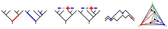
Figure 6. Connections between equivalent statistics. The descents of $S$ (resp. descents of $T$) on the left correspond to the positions where the canopies of $S$ and $T$ are both positive (resp. negative) in the middle left, to the double falls of $\pi(S)$ (resp. the valleys of $\pi(T)$) in the middle right, and to the intermediate nodes of the tree $T_{0}$ (resp. $T_{1}$) on the right.

Lemma 29.

For any binary trees $S$ and $T$,

1. the number of $-$ (resp. $+$) entries in the canopy of $T$ is given by $\operatorname{asc}(T)$ (resp. by $\operatorname{des}(T)$).

2. if $S\leq T$ in Tamari order, then the canopy of $S$ is componentwise smaller than the canopy of $T$ for the natural order $-\leq+$,

3. if $S\leq T$, then the number of positions where the entries of the canopies of both $S$ and $T$ are $-$ (resp. $+$) is given by $\operatorname{asc}(T)$ (resp. by $\operatorname{des}(S)$).

Proof.

1. By the characterization (iv) of the canopy above, $\operatorname{can}(T)_{j}={-}$ if and only if there is an edge $i\to j+1$ for some $i\leq j$, which thus defines an ascent of $T$. Hence, the number of $-$ entries in $\operatorname{can}(T)$ is $\operatorname{asc}(T)$. By symmetry, the number of $+$ entries in $\operatorname{can}(T)$ is $\operatorname{des}(T)$

2. It is sufficient to prove (ii) for a cover relation in the Tamari order. If the edge $i\to j$ with $i<j$ is rotated, then the canopy is unchanged, except maybe its $i$th entry, which changes from $-$ to $+$ when $j=i+1$. An alternative global argument is to observe that if $S\leq T$, then any linear extension of $S$ is smaller than any linear extension of $T$, so that there cannot be both oriented paths from $i+1$ to $i$ in $S$ and from $i$ to $i+1$ in $T$, and to use the characterization (ii) of the canopy above.

3. We have $\operatorname{can}(S)_{j}=\operatorname{can}(T)_{j}={-}$ if and only if $\operatorname{can}(T)_{j}={-}$ (by (ii)), so that the number of such positions is $\operatorname{asc}(T)$ by (i). By symmetry, the number of positions $j$ with $\operatorname{can}(S)_{j}=\operatorname{can}(T)_{j}={+}$ is $\operatorname{des}(S)$. ∎

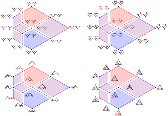
Figure 7. The decomposition of the cellular diagonal $\Delta_{2}$ of Figure 2, labeled using the equivalent statistics of Figure 6.

Using Lemma 29, we can transpose Theorems 1 and 2 in terms of canopy. We denote by $\operatorname{agr}(S,T)$ the number of canopy agreements between two binary trees $S$ and $T$ (i.e. of positions where the entries of the canopies of $S$ and $T$ agree).

Corollary 30.

For any $n,k\in\mathbb{N}$, we have

$$|\left\{S\leq T\;\middle|\;\operatorname{agr}(S,T)=k\right\}|=|\left\{S\leq T\;\middle|\;\operatorname{des}(S)+\operatorname{asc}(T)=k\right\}|=\frac{2}{n(n+1)}\binom{n+1}{k+2}\binom{3n}{k},$$

where $S\leq T$ are intervals of the Tamari lattice $\mathrm{Tam}(n)$ on binary trees with $n$ nodes.

Corollary 31.

For any $n,k\in\mathbb{N}$, we have

$$\sum_{S\leq T}\binom{\operatorname{agr}(S,T)}{k}=\sum_{S\leq T}\binom{\operatorname{des}(S)+\operatorname{asc}(T)}{k}=\frac{2}{(3n+1)(3n+2)}\binom{n-1}{k}\binom{4n+1-k}{n+1},$$

where the sums range over the intervals $S\leq T$ of the Tamari lattice $\mathrm{Tam}(n)$ on binary trees with $n$ nodes.

Remark 32.

For $k=n-1$ in both Corollaries 30 and 31, we recover that the number of synchronized Tamari intervals (i.e. with $\operatorname{agr}(S,T)=n-1$) is given by

$$\frac{2}{n(n+1)}\binom{3n}{n-1}=\frac{2}{(n+1)(2n+1)}\binom{3n}{n}=\frac{2}{(3n+1)(3n+2)}\binom{3n+2}{n+1}.$$

Remark 33.

Note that the first equalities of Corollaries 30 and 31 follow from [Cha18, Sect. 5]. The approach of [Cha18, Sect. 5] is however a bit of a detour as it passes again through generating functions, when the simple observation of Lemma 29 (iii) suffices.

6.1.2. Dyck paths

Recall that a Dyck path of semilength $n$ is a path from $(0,0)$ to $(2n,0)$ using $n$ up steps $(1,1)$ (denoted $U$) and $n$ down steps $(1,-1)$ (denoted $D$) and never passing below the horizontal axis. We denote by $\pi$ the standard bijection from binary trees to Dyck paths. Namely, the Dyck path $\pi(T)$ corresponding to a binary tree $T$ is obtained by walking clockwise around the contour of $T$ and marking an $U$ step when finding a leaf and a $D$ step when walking back an edge $j\to i$ with $i<j$. Note that $\pi$ transports the rotation on binary trees to the Tamari shift on Dyck paths, which exchanges a $D$ step preceding an $U$ step with the corresponding excursion (meaning the longest subpath which stays above this $U$ step). See Figures 6 and 7 for illustrations. The following lemma is classical and immediate.

Lemma 34.

The bijection $\pi$ from binary trees to Dyck path sends:

• the ascents of $T$ to the valleys of $\pi(T)$ (a $D$ step followed by an $U$ step),

• the descents of $T$ to the double falls of $\pi(T)$ (two consecutive $D$ steps),

• the edges on the left branch of $T$ to the contacts of $\pi(T)$ (its points on the horizontal axis).

Using Lemma 34, we can transpose Theorems 1 and 2 in terms of Dyck paths. We denote by $\operatorname{val}(P)$ (resp. $\operatorname{df}(P)$) the number of valleys (resp. of double falls) of a Dyck path $P$.

Corollary 35.

For any $n,k\in\mathbb{N}$, we have

$$|\left\{P\leq Q\;\middle|\;\operatorname{df}(P)+\operatorname{val}(Q)=k\right\}|=\frac{2}{n(n+1)}\binom{n+1}{k+2}\binom{3n}{k},$$

where $P\leq Q$ are intervals of the Tamari lattice $\mathrm{Tam}(n)$ on Dyck paths of semilength $n$.

Corollary 36.

For any $n,k\in\mathbb{N}$, we have

$$\sum_{P\leq Q}\binom{\operatorname{df}(P)+\operatorname{val}(Q)}{k}=\frac{2}{(3n+1)(3n+2)}\binom{n-1}{k}\binom{4n+1-k}{n+1},$$

where the sum ranges over the intervals $P\leq Q$ of the Tamari lattice $\mathrm{Tam}(n)$ on Dyck paths of semilength $n$.

6.1.3. Triangulations and minimal realizers

We now consider the bijection of [BB09] from Tamari intervals to rooted triangulations using Schnyder woods. Schnyder woods were introduced in [Sch89] for straightline embedding purposes, and the structure of Schnyder woods was investigated in particular in [OdM94, Pro97, Fel04b]. We refer to [Fel04a, Chap. 2] for a nice pedagogical presentation of Schnyder woods and their applications.

Recall that a planar map $M$ is an embedding of a planar graph on the sphere, considered up to continuous deformations. A face of $M$ is a connected component of the complement of $M$, and a corner is a pair of consecutive edges around a vertex. A rooted map is a map where a root corner is marked. The face containing this corner is then considered as the external face, and the vertices and edges of this external face are the external vertices and edges. A triangulation is a map where all faces have degree $3$. Euler formula implies that a rooted triangulation with $n$ internal vertices has $3n$ internal edges and $2n+1$ internal triangles.

Consider a rooted triangulation $M$ and denote by $v_{0},v_{1},v_{2}$ the external vertices of $M$ counterclockwise around the external face, and by $U$ the internal vertices of $M$. A realizer (or Schnyder wood [Sch89]) of $M$ is an orientation and coloring with colors $\{0,1,2\}$ of the edges of $M$ such that

• for each $i\in\{0,1,2\}$, the $i$-edges form a tree with vertices $U\cup\{v_{i}\}$ oriented towards $v_{i}$,

• counterclockwise around each internal vertex, we see a $0$-source, some $2$-targets, a $1$-source, some $0$-targets, a $2$-source, and some $1$-targets. (Note that some means possibly none.)

(An $i$-edge is an edge colored $i$, and an $i$-source or $i$-target is the source or target of and $i$-edge.) A realizer is minimal (resp. maximal) if it contains no clockwise (resp. counterclockwise) cycle. It was observed in [OdM94, Pro97, Fel04b] that the Schnyder woods on a given triangulation $M$ have the structure of a distributive lattice, where the cover relations correspond to reorientation of certain clockwise cycles. This has the following immediate consequence.

Theorem 37 ([OdM94, Pro97, Fel04b]).

Every triangulation has a unique minimal (resp. maximal) realizer.

Consider now a realizer $(T_{0},T_{1},T_{2})$ of a rooted triangulation $M$. Walking clockwise around $T_{0}$, we define two Dyck paths $P$ and $Q$ as follows:

• $P$ has an $U$ (resp. $D$) step each time we move farther from $v_{0}$ (resp. closer to $v_{0}$),

• $Q$ has an $U$ step each time we move farther from $v_{0}$ (except the first step), and a $D$ step each time we pass a $1$-target.

See Figures 6 and 7 for illustrations. This map was defined in [BB09], where it is proved that it behaves very nicely with respect to three lattice structures on Dyck paths (the Stanley lattice, the Tamari lattice and the Kreweras lattice). Here, we will use only the connection to the Tamari lattice, but we previously make an immediate observation. We call intermediate nodes of a rooted tree $T$ the nodes which are neither the root, nor the leaves of $T$.

Lemma 38.

Consider the pair $(P,Q)$ of Dyck paths obtained from a realizer $(T_{0},T_{1},T_{2})$. Then

• the double falls of $P$ correspond to the intermediate nodes of $T_{0}$,

• the valleys of $Q$ correspond to the intermediate nodes of $T_{1}$,

• the contacts of $P$ correspond to the corners of edges of $T_{0}$ incident to $v_{0}$.

We now restrict to minimal realizers to obtain a bijection between rooted triangulations and Tamari intervals, as described in [BB09]. We denote by $\operatorname{bb}(M)$ the pair of Dyck paths $(P,Q)$ obtained from the minimal realizer of $M$.

Theorem 39 ([BB09]).

The map $\operatorname{bb}$ is a bijection from rooted triangulations with $n$ internal vertices to the intervals of the Tamari lattice on Dyck paths of semilength $n$.

Using Lemmas 38 and 39, we can transpose Theorems 1 and 2 in terms of maps. For a rooted triangulation $M$, with minimal realizer $(T_{0},T_{1},T_{2})$, we denote by $\operatorname{inodes}(M)$ the number of intermediate nodes of $T_{0}$ plus the number of intermediate nodes of $T_{1}$.

Corollary 40.

For any $n,k\in\mathbb{N}$, we have

$$|\left\{M\;\middle|\;\operatorname{inodes}(M)=k\right\}|=\frac{2}{n(n+1)}\binom{n+1}{k+2}\binom{3n}{k},$$

where the $M$’s are the rooted triangulations with $n$ internal vertices.

Corollary 41.

For any $n,k\in\mathbb{N}$, we have

$$\sum_{M}\binom{\operatorname{inodes}(M)}{k}=\frac{2}{(3n+1)(3n+2)}\binom{n-1}{k}\binom{4n+1-k}{n+1},$$

where the sums range over all rooted triangulations $M$ with $n$ internal vertices.

6.2. Theorem 1 from triangulations

We now derive Theorem 1 from triangulations using the following result of [FH19]. It was obtained via a bijection from planar triangulations endowed with their minimal realizers to planar mobiles. We state it here in terms of canopies of binary trees.

Theorem 42 ([FH19, Coro. 2]).

Let $f_{i,j,k}$ denote the number of Tamari intervals $S\leq T$ with $i$ positions $p$ where $\operatorname{can}(S)_{p}=\operatorname{can}(T)_{p}={-}$, with $j$ positions $p$ where $\operatorname{can}(S)_{p}=\operatorname{can}(T)_{p}={+}$, and with $k$ positions $p$ where $\operatorname{can}(S)_{p}={-}$ while $\operatorname{can}(T)_{p}={+}$. Then the corresponding generating function $F\mbox{\,\raisebox{0.86108pt}{\scriptsize$\mathrm{:}$}$=$\,}F(u,v,w)\mbox{\,\raisebox{0.86108pt}{\scriptsize$\mathrm{:}$}$=$\,}\sum_{i,j,k}f_{i,j,k}u^{i}v^{j}w^{k}$ is given by

$$uvF=uU+vV+wUV-\frac{UV}{(1+U)(1+V)},$$

where the series $U\mbox{\,\raisebox{0.86108pt}{\scriptsize$\mathrm{:}$}$=$\,}U(u,v,w)$ and $V\mbox{\,\raisebox{0.86108pt}{\scriptsize$\mathrm{:}$}$=$\,}V(u,v,w)$ satisfy the system

$$U =(v+wU)(1+U)(1+V)^{2}$$

$$V =(u+wV)(1+V)(1+U)^{2}.$$

Corollary 43.

The generating function $A\mbox{\,\raisebox{0.86108pt}{\scriptsize$\mathrm{:}$}$=$\,}A(t,z)\mbox{\,\raisebox{0.86108pt}{\scriptsize$\mathrm{:}$}$=$\,}\sum a_{n,k}t^{n}z^{k}$ is given by

(18) $$tz^{2}A=2tzS+tS^{2}-\frac{S^{2}}{(1+S)^{2}},$$

where the series $S\mbox{\,\raisebox{0.86108pt}{\scriptsize$\mathrm{:}$}$=$\,}S(t,z)$ satisfies

(19) $$S=t(z+S)(1+S)^{3}.$$

Proof.

By Corollary 30, we have $A(t,z)=tF(tz,tz,t)$. Specializing $u=v=tz$ and $w=t$ in Theorem 42, we thus obtain the expression for $A(t,z)$ by observing that the series $U(tz,tz,t)$ and $V(tz,tz,t)$ coincide and denoting $S(t,z)\mbox{\,\raisebox{0.86108pt}{\scriptsize$\mathrm{:}$}$=$\,}U(tz,tz,t)=V(tz,tz,t)$. ∎

Differentiating Equation 18 with respect to the variable $t$, we obtain

$$\frac{\partial}{\partial t}(tz^{2}A) =2zS+2tz\frac{\partial S}{\partial t}+S^{2}+2tS\frac{\partial S}{\partial t}-\frac{2S}{(1+S)^{2}}\frac{\partial S}{\partial t}+\frac{2S^{2}}{(1+S)^{3}}\frac{\partial S}{\partial t}$$

$$=2zS+S^{2}+\frac{2}{(1+S)^{3}}\frac{\partial S}{\partial t}\Big{(}t(z+S)(1+S)^{3}-S(1+S)+S^{2}\Big{)}$$

(20) $$=2zS+S^{2},$$

where the last equality follows from Equation 19.

We obtain by Lagrange inversion in Equation 19 that for $r\geq 1$,

$$[t^{n}z^{k}]S^{r}=\frac{r}{n}[s^{n-r}z^{k}]\phi(s)^{n},$$

where $\phi(s)\mbox{\,\raisebox{0.86108pt}{\scriptsize$\mathrm{:}$}$=$\,}(z+s)(1+s)^{3}$. Thus

$$[t^{n}z^{k}]S^{r}=\frac{r}{n}[s^{n-r}z^{k}](z+s)^{n}(1+s)^{3n}=\frac{r}{n}\binom{n}{k}\binom{3n}{k-r}.$$

Hence, Equation 20 implies that

$$a_{n,k}=[t^{n}z^{k}]A=\frac{1}{n+1}[t^{n}z^{k+2}]\frac{\partial}{\partial t}(tz^{2}A)=\frac{1}{n+1}\big{(}2[t^{n}z^{k+1}]S+[t^{n}z^{k+2}]S^{2}\big{)}$$

is given by

$$\frac{2}{n(n+1)}\left(\binom{n}{k+1}+\binom{n}{k+2}\right)\binom{3n}{k}=\frac{2}{n(n+1)}\binom{n+1}{k+2}\binom{3n}{k}.$$

Remark 44.

In fact, the recent direct bijection of [FFN23] between Tamari intervals and blossoming trees enables to obtain Theorem 1 in an even simpler way. Details will appear in [FFN23].

7. Additional remarks

We conclude the paper with a few additional observations and comments on Theorems 1 and 2. We first discuss the (im)possibility to refine our formulas (Section 7.1), either by adding the statistics $\ell(S)$ (Section 7.1.1), or by separating the statistics $\operatorname{des}(S)$ and $\operatorname{asc}(T)$ (Section 7.1.2). We then provide a formula for the number of internal faces of the cellular diagonal of the associahedron (Section 7.2) which specializes on the one hand to the number of new Tamari intervals and on the other hand to the number of synchronized Tamari intervals of [Cha07]. We then discuss the problem to extend our results to $m$-Tamari lattice (Section 7.3). We conclude with an observation concerning decompositions of the cellular diagonal of the associahedron (Section 7.4).

7.1. (Im)possible refinements

We now discuss two tempting refinements of the formulas of Theorems 1 and 2, but observe that they seem not to give interesting formulas.

7.1.1. Adding $\ell(S)$

In Section 2, we used the number $\ell(S)$ of edges along the left branch of $S$ to define the catalytic variable $u$ leading to the functional equation on $A(t,z)$. It is known that the number of Tamari intervals $S\leq T$ with $n(S)=n(T)=n$ and $\ell(S)=i$ is given by the formula

$$\frac{(i-1)(4n-2i+1)!}{(3n-i+2)!(n-i+1)!}\binom{2i}{i}.$$

These numbers appear as [OEI10, A146305], see Table 3 for the first few values. They also count the rooted $3$-connected triangulations with $n+3$ vertices and $i$ vertices adjacent to the root vertex.

In view of this formula, it is tempting to try to refine Theorems 1 and 2 by incorporating the additional parameter $\ell(S)$. Indeed, it is natural to consider the numbers $a_{n,i,k}$ of intervals ${S\leq T}$ of the Tamari lattice $\mathrm{Tam}(n)$ such that $\ell(S)=i$ and $\operatorname{des}(S)+\operatorname{asc}(T)=k$, as well as the numbers $b_{n,i,k}=\sum_{\ell=k}^{n-1}a_{n,i,\ell}\binom{\ell}{k}$. These numbers are gathered in Tables 7 and 8. Unfortunately, some of these numbers have big prime factors, which discards the possibility to find simple product formulas.

$n\backslash k$	$0$	$1$	$2$	$3$	$4$	$5$	$6$	$7$	$8$	$\Sigma$
$1$	$1$									$1$
$2$	$1$	$2$								$3$
$3$	$3$	$5$	$5$							$13$
$4$	$13$	$20$	$21$	$14$						$68$
$5$	$68$	$100$	$105$	$84$	$42$					$399$
$6$	$399$	$570$	$595$	$504$	$330$	$132$				$2530$
$7$	$2530$	$3542$	$3675$	$3192$	$2310$	$1287$	$429$			$16965$
$8$	$16965$	$23400$	$24150$	$21252$	$16170$	$10296$	$5005$	$1430$		$118668$
$9$	$118668$	$161820$	$166257$	$147420$	$115500$	$78936$	$45045$	$19448$	$4862$	$857956$

Table 3. The first few values of $\frac{(i-1)(4n-2i+1)!}{(3n-i+2)!(n-i+1)!}\binom{2i}{i}$ [OEI10, A146305].

7.1.2. Separating $\operatorname{des}(S)$ and $\operatorname{asc}(T)$

It was conjectured in [Cha18, Sec. 2] that the number of Tamari intervals $S\leq T$ with $n(S)=n(T)=n$, $\operatorname{des}(S)=p$ and $\operatorname{asc}(T)=n-p-1$ is given by the formula

$$\frac{(n+p-1)!(2n-p)!}{p!(n+1-p)!(2p-1)!(2n-2p+1)!}.$$

These numbers appear as [OEI10, A082680], see Table 4 for the first few values. They also count the $2$-stack sortable permutations of $[n]$ with $p$ runs [Bón97].

$n\backslash p$	$0$	$1$	$2$	$3$	$4$	$5$	$6$	$7$	$8$	$\Sigma$
$1$	$1$									$1$
$2$	$1$	$1$								$2$
$3$	$1$	$4$	$1$							$6$
$4$	$1$	$10$	$10$	$1$						$22$
$5$	$1$	$20$	$49$	$20$	$1$					$91$
$6$	$1$	$35$	$168$	$168$	$35$	$1$				$408$
$7$	$1$	$56$	$462$	$900$	$462$	$56$	$1$			$1938$
$8$	$1$	$84$	$1092$	$3630$	$3630$	$1092$	$84$	$1$		$9614$
$9$	$1$	$120$	$2310$	$12012$	$20449$	$12012$	$2310$	$120$	$1$	$49335$

Table 4. The first few values of $\frac{(n+p-1)!(2n-p)!}{p!(n+1-p)!(2p-1)!(2n-2p+1)!}$ [OEI10, A082680].

In view of this formula, it is tempting to try to refine Theorems 1 and 2 by separating $\operatorname{des}(S)$ and $\operatorname{asc}(T)$. For Theorem 1, it is natural to consider the numbers of intervals $S\leq T$ of the Tamari lattice $\mathrm{Tam}(n)$ such that $\operatorname{des}(S)=p$ and $\operatorname{asc}(T)=q$. These numbers are gathered in Table 9, which was already considered in [Cha18, Sect. 5]. For Theorem 2, there are three possible refinements:

1. Either consider the number of faces of $\Delta_{n-1}$ corresponding to pairs $(F,G)$ of faces of the associahedron with $\dim(F)=p$ and $\dim(G)=q$. These numbers are gathered in Table 10.

2. Or consider the sums $\sum_{S\leq T}\binom{\operatorname{des}(S)+\operatorname{asc}(T)}{k}$ over all Tamari intervals with ${n(S)=n}$ and $\operatorname{des}(S)=p$. These numbers are gathered in Table 11.

3. Or consider the sums $\sum_{S\leq T}\binom{\operatorname{des}(S)+\operatorname{asc}(T)}{k}$ over all Tamari intervals with $n(S)=n$, $\operatorname{des}(S)=p$ and $\operatorname{asc}(T)=q$. For instance, for $n=4$ we obtain the numbers in Table 12.

Again, these numbers have big prime factors, which discards the possibility to find simple product formulas.

7.2. Internal faces of the cellular diagonal and new intervals

Another interesting direction is to consider the internal faces of the cellular diagonal, i.e. the faces that appear in the interior of the associahedron. The first few values are gathered in Table 5. Note that these numbers have two relevant specializations.

1. The internal vertices of $\Delta_{n-1}$ correspond to new Tamari intervals from [Cha07, Sect. 7] (intervals that cannot be obtained by replacing each node by a Tamari interval in a Schröder tree), and are enumerated by

   $$\frac{3\cdot 2^{n-2}}{n(n+1)}\binom{2n-2}{n-1}.$$

   This formula was proved in [Cha07, Thm. 9.1] and appears as [OEI10, A000257]. It also counts bipartite planar maps with $n-1$ edges, and an explicit bijection between new intervals and bipartite planar maps was given in [Fan21].

2. All facets of $\Delta_{n-1}$ are internal and correspond to synchronized Tamari intervals, enumerated by

   $$\frac{2}{(n+1)(2n+1)}\binom{3n}{n}$$

   This formula was proved in [FPR17] and appears as [OEI10, A000139]. It also counts the rooted non-separable planar maps with $n+1$ edges, and the $2$-stack sortable permutations of $[n]$, among others.

In view of these two specializations, it is tempting to count the internal faces of the cellular diagonal. We start with an immediate characterization.

Lemma 45.

The face of the associahedron corresponding to a Schröder tree $E$ contains the face of $\Delta_{n-1}$ corresponding to a pair $(F,G)$ of Schröder trees if and only if $E$ is a contraction of both $F$ and $G$.

From Lemma 45, we can adapt the approach of Proposition 7 to count all internal faces of $\Delta_{n-1}$. Fix a Tamari interval $S\leq T$. We say that a descent edge $s$ of $S$ is free (resp. constrained, resp. tied) if there is no edge (resp. an ascent edge, resp. a descent edge) $t$ in $T$ such that the contraction of all edges but $s$ in $S$ coincides with the contraction of all edges but $t$ in $T$. We define similarly the free, contrained and tied ascent edges of $T$. We denote by $\operatorname{free}(S,T)$ the numbers of free descents of $S$ plus the number of free ascents of $T$, by $\operatorname{tied}(S,T)$ the number of tied descents of $S$ plus the number of tied ascents of $T$, and by $\operatorname{const}(S,T)$ the number of constrained descents of $S$ or equivalently of constrained ascents of $T$.

Proposition 46.

The number of internal $k$-dimensional faces of the cellular diagonal $\Delta_{n-1}$ of the $(n-1)$-dimensional associahedron is given by

$$\sum_{S\leq T}\sum_{i}2^{i}\binom{\operatorname{const}(S,T)}{i}\binom{\operatorname{free}(S,T)}{k-\operatorname{tied}(S,T)-2\operatorname{const}(S,T)+i},$$

where the sums range over the intervals $S\leq T$ of the Tamari lattice $\mathrm{Tam}(n)$ on binary trees with $n$ nodes.

Proof.

We still associate each face $(F,G)$ of $\Delta_{n-1}$ to the Tamari interval $S\leq T$ where ${S=\max(F)}$ and $T=\min(G)$. The $k$-dimensional faces associated to a Tamari interval $S\leq T$ are thus obtained by contracting $\ell$ descent edges of $S$ and $k-\ell$ ascent edges of $T$ for some $0\leq\ell\leq k$. Such a face is internal if and only if we contract all tied descents edges of $S$ and tied ascent edges of $T$, at least one edge among each pair of constrained edges, and possibly some free ascent edges of $S$ and free descent edges of $T$. We thus immediately obtain the formula, where $i$ denotes the number of pairs of constrained edges where only one edge is contracted. ∎

The first few values of the formula of Proposition 46 are gathered in Table 5. Again, except the first column and the diagonal, these numbers have big prime factors, which discards the possibility to find a simple product formula.

$n\backslash k$	$0$	$1$	$2$	$3$	$4$	$5$	$6$	$\Sigma$
$1$	$1$							$1$
$2$	$1$	$2$						$3$
$3$	$3$	$8$	$6$					$17$
$4$	$12$	$42$	$51$	$22$				$127$
$5$	$56$	$244$	$406$	$308$	$91$			$1105$
$6$	$288$	$1504$	$3171$	$3384$	$1836$	$408$		$10591$
$7$	$1584$	$9648$	$24606$	$33680$	$26145$	$10944$	$1938$	$108545$

Table 5. The number of internal $k$-dimensional faces of the cellular diagonal $\Delta_{n-1}$ of the $(n-1)$-dimensional associahedron. Note that the first column is [OEI10, A000257] while the diagonal is [OEI10, A000139].

7.3. $m$-Tamari lattices

The $m$-Tamari lattice $\mathrm{Tam}(m,n)$ was originally defined in [BPR12] in the context of multivariate diagonal harmonics as the lattice whose

• elements are the paths consisting of north steps $(0,1)$ (denoted $N$) and east steps $(1,0)$ (denoted $E$), starting at $(0,0)$, ending at $(mn,n)$, and remaining above the line $x=my$,

• cover relations exchange a $N$ step followed by an $E$ step with the corresponding excursion (meaning the smallest factor with $m$ times more $E$ than $N$ steps).

It was later observed in [BMFPR11] that it is isomorphic to the upper ideal of the Tamari lattice $\mathrm{Tam}(mn)$ generated by the path $(U^{m}D^{m})^{n}$. Another interpretation as a quotient of the $m$-sylvester congruence on $m$-permutations was also studied in [NT20, Pon15].

Note that the $m$-Tamari lattice naturally generalizes the Tamari lattice, as $\mathrm{Tam}(1,n)=\mathrm{Tam}(n)$. The number of elements of $\mathrm{Tam}(m,n)$ is the Fuss-Catalan number $\frac{1}{mn+1}\binom{(m+1)n}{n}$, generalizing the Catalan number. The number of intervals of $\mathrm{Tam}(m,n)$ is given by the product formula

$$\frac{m+1}{n(mn+1)}\binom{(m+1)^{2}n+m}{n-1},$$

proved in [BMFPR11] and generalizing the formula of [Cha07] for the Tamari lattice. See Table 6 for the first few values. This formula can even be refined by the number of contacts with the $x=my$ line, generalizing the formula of Section 7.1.1. See [BMFPR11, Coro. 11].

$n\backslash m$	$1$	$2$	$3$	$4$	$5$	$6$
$1$	$1$	$1$	$1$	$1$	$1$	$1$
$2$	$3$	$6$	$10$	$15$	$21$	$28$
$3$	$13$	$58$	$170$	$395$	$791$	$1428$
$4$	$68$	$703$	$3685$	$13390$	$38591$	$94738$
$5$	$399$	$9729$	$91881$	$524256$	$2180262$	$7291550$
$6$	$2530$	$146916$	$2509584$	$22533126$	$135404269$	$617476860$
$7$	$16965$	$2359968$	$73083880$	$1033921900$	$8984341696$	$55896785092$
$8$	$118668$	$39696597$	$2232019920$	$49791755175$	$625980141828$	$5315230907547$
$9$	$857956$	$691986438$	$70714934290$	$2488847272300$	$45284778249165$	$524898029145217$

Table 6. The first few values of $\frac{m+1}{n(mn+1)}\binom{(m+1)^{2}n+m}{n-1}$.

It is tempting to look for analogues of Theorems 1 and 2 for $m$-Tamari lattices. However, it is unclear to us how to generalize the statistics $\operatorname{des}(S)$ and $\operatorname{asc}(T)$. We have considered two options here: for an element $M$ of $\mathrm{Tam}(m,n)$, define

1. $\operatorname{des}(M)$ (resp. $\operatorname{asc}(M)$) as the number of elements of $\mathrm{Tam}(m,n)$ covered by (resp. covering) $M$,

2. $\operatorname{des}(M)$ (resp. $\operatorname{asc}(M)$) as the number of strong descents (resp. ascents) in any permutation of the $m$-sylvester class corresponding to $M$ in the sense of [NT20, Pon15]. Here, a strong descent (resp. ascent) in an $m$-permutation is an index $i$ such that all the occurrences of $i$ appear after (resp. before) all occurrences of $i+1$.

The numbers of $m$-Tamari intervals $M\leq N$ with $\operatorname{des}(M)+\operatorname{asc}(N)=k$ for these two definitions are gathered in Tables 13 and 14. Note that, for an interval $M\leq N$ in $\mathrm{Tam}(m,n)$, the sum ${\operatorname{des}(M)+\operatorname{asc}(N)}$ can be as big as $mn-1$ for the first definition, but is bounded by $n-1$ for the second definition. Finally, another option is to consider the number of canopy agreements between $M$ and $N$, generalizing the interpretation of Section 6.1.1. Here, the canopy can be defined as the position of the block of occurrences of $i$ in the occurrences of $i+1$ in any $m$-permutation corresponding to $M$. The numbers of $m$-Tamari intervals $M\leq N$ with $k$ canopy agreements are gathered in Table 15. Unfortunately, the numbers in Tables 13, LABEL:, 14, LABEL: and 15 do not factorize nicely.

7.4. Other decompositions of the cellular diagonal

We conclude with an observation concerning the rightmost picture of Figure 2. This picture is a decomposition of $\Delta_{2}$, where each face $(F,G)$ is associated to the Tamari interval $\max(F)\leq\min(G)$. In fact, there are $4$ natural ways to decompose the cellular diagonal $\Delta_{n-1}$ of the $(n-1)$-dimensional associahedron. Namely, we can associate each face $(F,G)$ of $\Delta_{n-1}$ with either of the intervals

$$\min(F)\leq\min(G),\quad\min(F)\leq\max(G),\quad\max(F)\leq\min(G),\quad\text{or}\quad\max(F)\leq\max(G).$$

These $4$ possible decompositions of $\Delta_{2}$ are illustrated in Figure 8. Note that all but the choice $\min(F)\leq\max(G)$ provide valid Morse functions that enable to count the $f$-vector of $\Delta_{n-1}$ using a binomial transform, as in the proof of Proposition 7.

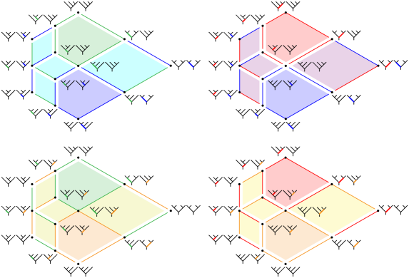
Figure 8. The four natural ways to associate a Tamari interval to each face $(F,G)$ of the cellular diagonal $\Delta_{2}$: using either $\min(F)\leq\min(G)$ (top left), or $\max(F)\leq\min(G)$ (top right), or $\min(F)\leq\max(G)$ (bottom left), or $\max(F)\leq\max(G)$ (bottom right). In this paper, we use $\max(F)\leq\min(G)$ (top right).

Aknowledgements

VP thanks all participants of the “2023 Barcelona Workshop: Homotopy theory meets polyhedral combinatorics” (Mónica Blanco, Luis Crespo, Guillaume Laplante-Anfossi, Arnau Padrol, Eva Philippe, Julian Pfeifle, Daria Poliakova, Francisco Santos and Andy Tonks) where the question to understand the $f$-vector of the cellular diagonal of the associahedron was raised. VP is particularly grateful to Guillaume Laplante-Anfossi for various discussions on the cellular diagonal of the associahedron and for an amazing number of suggestions on the presentation of the paper, and to Francisco Santos for suggesting the rightmost picture of Figure 2. VP thanks Éric Fusy for suggesting the bijective approach of Section 6.2 and answering technical questions on this approach. VP also thanks Frédéric Chapoton, Florent Hivert and Gilles Schaeffer for interesting discussions and inputs on this paper.

$n=1$ $n=2$ $n=3$ $n=4$ $n=5$ $i\backslash k$ $0$ $\Sigma$ $0$ $1$ $1$ $\Sigma$ $1$ $i\backslash k$ $0$ $1$ $\Sigma$ $0$ $0$ $1$ $1$ $1$ $1$ $1$ $2$ $\Sigma$ $1$ $2$ $i\backslash k$ $0$ $1$ $2$ $\Sigma$ $0$ $0$ $1$ $2$ $3$ $1$ $0$ $2$ $3$ $5$ $2$ $1$ $3$ $1$ $5$ $\Sigma$ $1$ $6$ $6$ $i\backslash k$ $0$ $1$ $2$ $3$ $\Sigma$ $0$ $0$ $1$ $6$ $6$ $13$ $1$ $0$ $2$ $9$ $9$ $20$ $2$ $0$ $3$ $12$ $6$ $21$ $3$ $1$ $6$ $6$ $1$ $14$ $\Sigma$ $1$ $12$ $33$ $22$ $i\backslash k$ $0$ $1$ $2$ $3$ $4$ $\Sigma$ $0$ $0$ $1$ $12$ $33$ $22$ $68$ $1$ $0$ $2$ $19$ $47$ $32$ $100$ $2$ $0$ $3$ $24$ $52$ $26$ $105$ $3$ $0$ $4$ $30$ $40$ $10$ $84$ $4$ $1$ $10$ $20$ $10$ $1$ $42$ $\Sigma$ $1$ $20$ $105$ $182$ $91$

Table 7. The numbers $a_{n,i,k}$ of intervals $S\leq T$ of the Tamari lattice $\mathrm{Tam}(n)$ such that $\ell(S)=i$ and $\operatorname{des}(S)+\operatorname{asc}(T)=k$ for small values of $n,i,k$.

$n=1$ $n=2$ $n=3$ $n=4$ $n=5$ $i\backslash k$ $0$ $0$ $1$ $\Sigma$ $1$ $i\backslash k$ $0$ $1$ $0$ $1$ $1$ $1$ $2$ $1$ $\Sigma$ $3$ $2$ $i\backslash k$ $0$ $1$ $2$ $0$ $3$ $5$ $2$ $1$ $5$ $8$ $3$ $2$ $5$ $5$ $1$ $\Sigma$ $13$ $18$ $6$ $i\backslash k$ $0$ $1$ $2$ $3$ $0$ $13$ $31$ $24$ $6$ $1$ $20$ $47$ $36$ $9$ $2$ $21$ $45$ $30$ $6$ $3$ $14$ $21$ $9$ $1$ $\Sigma$ $68$ $144$ $99$ $22$ $i\backslash k$ $0$ $1$ $2$ $3$ $4$ $0$ $68$ $212$ $243$ $121$ $22$ $1$ $100$ $309$ $352$ $175$ $32$ $2$ $105$ $311$ $336$ $156$ $26$ $3$ $84$ $224$ $210$ $80$ $10$ $4$ $42$ $84$ $56$ $14$ $1$ $\Sigma$ $399$ $1140$ $1197$ $546$ $91$

Table 8. The numbers $b_{n,i,k}=\sum_{\ell=k}^{n-1}a_{n,i,\ell}\binom{\ell}{k}$ for small values of $n,i,k$.

$n=1$ $n=2$ $n=3$ $n=4$ $n=5$ $p\backslash q$ $0$ $0$ $1$ $p\backslash q$ $0$ $1$ $0$ $1$ $1$ $1$ $1$ $p\backslash q$ $0$ $1$ $2$ $0$ $1$ $3$ $1$ $1$ $3$ $4$ $2$ $1$ $p\backslash q$ $0$ $1$ $2$ $3$ $0$ $1$ $6$ $6$ $1$ $1$ $6$ $21$ $10$ $2$ $6$ $10$ $3$ $1$ $p\backslash q$ $0$ $1$ $2$ $3$ $4$ $0$ $1$ $10$ $20$ $10$ $1$ $1$ $10$ $65$ $81$ $20$ $2$ $20$ $81$ $49$ $3$ $10$ $20$ $4$ $1$

Table 9. The numbers of intervals $S\leq T$ of the Tamari lattice $\mathrm{Tam}(n)$ such that $\operatorname{des}(S)=p$ and $\operatorname{asc}(T)=q$ for small values of $n,p,q$.

$n=1$ $n=2$ $n=3$ $n=4$ $n=5$ $p\backslash q$ $0$ $0$ $1$ $p\backslash q$ $0$ $1$ $0$ $3$ $1$ $1$ $1$ $p\backslash q$ $0$ $1$ $2$ $0$ $13$ $9$ $1$ $1$ $9$ $4$ $2$ $1$ $p\backslash q$ $0$ $1$ $2$ $3$ $0$ $68$ $72$ $19$ $1$ $1$ $72$ $61$ $10$ $2$ $19$ $10$ $3$ $1$ $p\backslash q$ $0$ $1$ $2$ $3$ $4$ $0$ $399$ $570$ $246$ $34$ $1$ $1$ $570$ $705$ $239$ $20$ $2$ $246$ $239$ $49$ $3$ $34$ $20$ $4$ $1$

Table 10. The numbers of pairs $(F,G)$ of faces of the $(n-1)$-dimensional associahedron with $\max(F)\leq\min(G)$ and $\dim(F)=p$ and $\dim(G)=q$ for small values of $n,p,q$.

$n=1$ $n=2$ $n=3$ $n=4$ $n=5$ $\ell\backslash k$ $0$ $0$ $1$ $\Sigma$ $1$ $\ell\backslash k$ $0$ $1$ $0$ $2$ $1$ $1$ $1$ $1$ $\Sigma$ $3$ $2$ $\ell\backslash k$ $0$ $1$ $2$ $0$ $5$ $5$ $1$ $1$ $7$ $11$ $4$ $2$ $1$ $2$ $1$ $\Sigma$ $13$ $18$ $6$ $\ell\backslash k$ $0$ $1$ $2$ $3$ $0$ $14$ $21$ $9$ $1$ $1$ $37$ $78$ $51$ $10$ $2$ $16$ $42$ $36$ $10$ $3$ $1$ $3$ $3$ $1$ $\Sigma$ $68$ $144$ $99$ $22$ $\ell\backslash k$ $0$ $1$ $2$ $3$ $4$ $0$ $42$ $84$ $56$ $14$ $1$ $1$ $176$ $463$ $428$ $161$ $20$ $2$ $150$ $479$ $557$ $227$ $49$ $3$ $30$ $110$ $150$ $90$ $20$ $4$ $1$ $4$ $6$ $4$ $1$ $\Sigma$ $399$ $1140$ $1197$ $546$ $91$

Table 11. The value of $\sum_{S\leq T}\delta_{\operatorname{des}(S)=p}\binom{\operatorname{des}(S)+\operatorname{asc}(T)}{k}$ for small values of $n,k,p$, and their sums over $p$ (which are the rows of Table 2).

$k=0$ $k=1$ $k=2$ $k=3$ $p\backslash q$ $0$ $1$ $2$ $3$ $0$ $1$ $6$ $6$ $1$ $1$ $6$ $21$ $10$ $2$ $6$ $10$ $3$ $1$ $p\backslash q$ $0$ $1$ $2$ $3$ $0$ $6$ $12$ $3$ $1$ $6$ $42$ $30$ $2$ $12$ $30$ $3$ $3$ $p\backslash q$ $0$ $1$ $2$ $3$ $0$ $6$ $3$ $1$ $21$ $30$ $2$ $6$ $30$ $3$ $3$ $p\backslash q$ $0$ $1$ $2$ $3$ $0$ $1$ $1$ $10$ $2$ $10$ $3$ $1$

Table 12. The value of $\sum_{S\leq T}\delta_{\operatorname{des}(S)=p}\delta_{\operatorname{asc}(T)=q}\binom{\operatorname{des}(S)+\operatorname{asc}(T)}{k}$ for $n=4$ and small values of $k,p,q$.

$m=1$ $m=2$ $n\backslash k$ $0$ $1$ $2$ $3$ $\Sigma$ $1$ $1$ $1$ $2$ $1$ $2$ $3$ $3$ $1$ $6$ $6$ $13$ $4$ $1$ $12$ $33$ $22$ $68$ $n\backslash k$ $0$ $1$ $2$ $3$ $4$ $5$ $6$ $\Sigma$ $1$ $1$ $1$ $2$ $1$ $4$ $1$ $6$ $3$ $1$ $12$ $30$ $14$ $1$ $58$ $4$ $1$ $24$ $150$ $306$ $189$ $32$ $1$ $703$ $m=3$ $m=4$ $n\backslash k$ $0$ $1$ $2$ $3$ $4$ $5$ $6$ $\Sigma$ $1$ $1$ $1$ $2$ $1$ $6$ $3$ $10$ $3$ $1$ $18$ $72$ $66$ $13$ $170$ $4$ $1$ $36$ $351$ $1196$ $1437$ $596$ $68$ $3685$ $n\backslash k$ $0$ $1$ $2$ $3$ $4$ $5$ $6$ $\Sigma$ $1$ $1$ $1$ $2$ $1$ $8$ $6$ $15$ $3$ $1$ $24$ $132$ $180$ $58$ $395$ $4$ $1$ $48$ $636$ $3036$ $5406$ $3560$ $703$ $13390$ $m=5$ $m=6$ $n\backslash k$ $0$ $1$ $2$ $3$ $4$ $5$ $6$ $\Sigma$ $1$ $1$ $1$ $2$ $1$ $10$ $10$ $21$ $3$ $1$ $30$ $210$ $380$ $170$ $791$ $4$ $1$ $60$ $1005$ $6170$ $14550$ $13120$ $3685$ $38591$ $n\backslash k$ $0$ $1$ $2$ $3$ $4$ $5$ $6$ $\Sigma$ $1$ $1$ $1$ $2$ $1$ $12$ $15$ $28$ $3$ $1$ $36$ $306$ $690$ $395$ $1428$ $4$ $1$ $72$ $1458$ $10942$ $32115$ $36760$ $13390$ $94738$

Table 13. The numbers of intervals $M\leq N$ of the $m$-Tamari lattice $\mathrm{Tam}(m,n)$ such that $\operatorname{des}(M)+\operatorname{asc}(N)=k$ for small values of $m,n,k$ (here, $\operatorname{des}(M)$ and $\operatorname{asc}(M)$ denote the number of elements of $\mathrm{Tam}(m,n)$ covered by and covering $M$).

$m=1$ $m=2$ $n\backslash k$ $0$ $1$ $2$ $3$ $\Sigma$ $1$ $1$ $1$ $2$ $1$ $2$ $3$ $3$ $1$ $6$ $6$ $13$ $4$ $1$ $12$ $33$ $22$ $68$ $n\backslash k$ $0$ $1$ $2$ $3$ $\Sigma$ $1$ $1$ $1$ $2$ $4$ $2$ $6$ $3$ $20$ $29$ $9$ $58$ $4$ $112$ $306$ $234$ $51$ $703$ $m=3$ $m=4$ $n\backslash k$ $0$ $1$ $2$ $3$ $\Sigma$ $1$ $1$ $1$ $2$ $8$ $2$ $10$ $3$ $85$ $72$ $13$ $170$ $4$ $1034$ $1763$ $786$ $102$ $3685$ $n\backslash k$ $0$ $1$ $2$ $3$ $\Sigma$ $1$ $1$ $1$ $2$ $13$ $2$ $15$ $3$ $233$ $144$ $18$ $395$ $4$ $4837$ $6380$ $1989$ $184$ $13390$

Table 14. The numbers of intervals $M\leq N$ of the $m$-Tamari lattice $\mathrm{Tam}(m,n)$ such that $\operatorname{des}(M)+\operatorname{asc}(N)=k$ for small values of $m,n,k$ (here, $\operatorname{des}(M)$ and $\operatorname{asc}(M)$ denote the number of strong ascents and descents in any $m$-permutation representing $M$).

$m=1$ $m=2$ $n\backslash k$ $0$ $1$ $2$ $3$ $\Sigma$ $1$ $1$ $1$ $2$ $1$ $2$ $3$ $3$ $1$ $6$ $6$ $13$ $4$ $1$ $12$ $33$ $22$ $68$ $n\backslash k$ $0$ $1$ $2$ $3$ $\Sigma$ $1$ $1$ $1$ $2$ $3$ $3$ $6$ $3$ $11$ $31$ $16$ $58$ $4$ $45$ $234$ $315$ $109$ $703$ $m=3$ $m=4$ $n\backslash k$ $0$ $1$ $2$ $3$ $\Sigma$ $1$ $1$ $1$ $2$ $6$ $4$ $10$ $3$ $48$ $90$ $32$ $170$ $4$ $441$ $1520$ $1391$ $333$ $3685$ $n\backslash k$ $0$ $1$ $2$ $3$ $\Sigma$ $1$ $1$ $1$ $2$ $10$ $5$ $15$ $3$ $140$ $200$ $55$ $395$ $4$ $2280$ $6050$ $4268$ $792$ $13390$

Table 15. The numbers of intervals $M\leq N$ of the $m$-Tamari lattice $\mathrm{Tam}(m,n)$ such that $k$ canopy agreements for small values of $m,n,k$.

References

- [AP22] Doriann Albertin and Vincent Pilaud. The canonical complex of the weak order. Order, 2022. online first.
- [APS04] George E. Andrews, Peter Paule, and Carsten Schneider. Plane partitions. VI. Stembridge’s TSPP theorem. RISC Report Series 04-08, Research Institute for Symbolic Computation (RISC), Johannes Kepler University Linz, Altenberger Straße 69, 4040 Linz, Austria, May 2004. 80 pages.
- [APS05] George E. Andrews, Peter Paule, and Carsten Schneider. Plane partitions. VI. Stembridge’s TSPP theorem. Adv. in Appl. Math., 34(4):709–739, 2005.
- [Bar19] Emily Barnard. The canonical join complex. Electron. J. Combin., 26(1):Paper No. 1.24, 25, 2019.
- [BB09] Olivier Bernardi and Nicolas Bonichon. Intervals in Catalan lattices and realizers of triangulations. J. Combin. Theory Ser. A, 116(1):55–75, 2009.
- [BLS17] Alin Bostan, Pierre Lairez, and Bruno Salvy. Multiple binomial sums. J. Symbolic Comput., 80(part 2):351–386, 2017.
- [BMFPR11] Mireille Bousquet-Mélou, Éric Fusy, and Louis-François Préville-Ratelle. The number of intervals in the -Tamari lattices. Electron. J. Combin., 18(2):Paper 31, 26, 2011.
- [Bón97] Miklós Bóna. -stack sortable permutations with a given number of runs. Preprint, arXiv:math/9705220v1, 1997.
- [BP96] Manuel Bronstein and Marko Petkovšek. An introduction to pseudo-linear algebra. Theoret. Comput. Sci., 157(1):3–33, 1996.
- [BPR12] François Bergeron and Louis-François Préville-Ratelle. Higher trivariate diagonal harmonics via generalized Tamari posets. J. Comb., 3(3):317–341, 2012.
- [BS92] Louis J. Billera and Bernd Sturmfels. Fiber polytopes. Ann. of Math. (2), 135(3):527–549, 1992.
- [Cha07] Frédéric Chapoton. Sur le nombre d’intervalles dans les treillis de Tamari. Sém. Lothar. Combin., 55:Art. B55f, 18, 2005/07.
- [Cha18] Frédéric Chapoton. Une note sur les intervalles de Tamari. Ann. Math. Blaise Pascal, 25(2):299–314, 2018.
- [Chy98] Frédéric Chyzak. Fonctions holonomes en Calcul formel. PhD thesis, École polytechnique, 1998.
- [CMSPT14] Frédéric Chyzak, Assia Mahboubi, Thomas Sibut-Pinote, and Enrico Tassi. A computer-algebra-based formal proof of the irrationality of . In Gerwin Klein and Ruben Gamboa, editors, Interactive Theorem Proving, number 8558 in Lecture Notes in Computer Science, pages 160–176, Vienna, Austria, 2014. Springer.
- [DLM] NIST Digital Library of Mathematical Functions. Published electronically at https://dlmf.nist.gov/, release 1.1.9 of 2023-03-15.
- [DOJVLA+23] Bérénice Delcroix-Oger, Mathieu Josuat-Vergès, Guillaume Laplante-Anfossi, Vincent Pilaud, and Kurt Stoeckl. The combinatorics of the permutahedron diagonals. In preparation, 2023.
- [Fan21] Wenjie Fang. Bijective link between Chapoton’s new intervals and bipartite planar maps. European J. Combin., 97:Paper No. 103382, 15, 2021.
- [Fel04a] Stefan Felsner. Geometric graphs and arrangements. Advanced Lectures in Mathematics. Friedr. Vieweg & Sohn, Wiesbaden, 2004. Some chapters from combinatorial geometry.
- [Fel04b] Stefan Felsner. Lattice structures from planar graphs. Electron. J. Combin., 11(1):Research Paper 15, 24, 2004.
- [FFN23] Wenjie Fang, Éric Fusy, and Philippe Nadeau. Bijections between Tamari intervals and blossoming trees. In preparation, 2023.
- [FH19] Éric Fusy and Abel Humbert. Bijections for generalized Tamari intervals via orientations. Preprint, arXiv:1906.11588, 2019.
- [FPR17] Wenjie Fang and Louis-François Préville-Ratelle. The enumeration of generalized Tamari intervals. European J. Combin., 61:69–84, 2017.
- [FS09] Philippe Flajolet and Robert Sedgewick. Analytic combinatorics. Cambridge University Press, Cambridge, 2009.
- [GJ04] Ian P. Goulden and David M. Jackson. Combinatorial enumeration. Dover Publications, Inc., Mineola, NY, 2004. With a foreword by Gian-Carlo Rota, Reprint of the 1983 original.
- [Har15] John Harrison. Formal proofs of hypergeometric sums. J. Automat. Reason., 55(3):223–243, 2015.
- [KP11] Manuel Kauers and Peter Paule. The concrete tetrahedron. Texts and Monographs in Symbolic Computation. SpringerWienNewYork, Vienna, 2011. Symbolic sums, recurrence equations, generating functions, asymptotic estimates.
- [Kur88] A. Kurosh. Higher algebra. “Mir”, Moscow, 1988. Translated from the Russian by George Yankovsky, Reprint of the 1972 translation.
- [LA22] Guillaume Laplante-Anfossi. The diagonal of the operahedra. Adv. Math., 405:Paper No. 108494, 50, 2022.
- [Lip89] L. Lipshitz. -finite power series. J. Algebra, 122(2):353–373, 1989.
- [Lod04] Jean-Louis Loday. Realization of the Stasheff polytope. Arch. Math. (Basel), 83(3):267–278, 2004.
- [Lod11] Jean-Louis Loday. The diagonal of the Stasheff polytope. In Higher structures in geometry and physics, volume 287 of Progr. Math., pages 269–292. Birkhäuser/Springer, New York, 2011.
- [MS06] Martin Markl and Steve Shnider. Associahedra, cellular -construction and products of -algebras. Trans. Amer. Math. Soc., 358(6):2353–2372, 2006.
- [MTTV21] Naruki Masuda, Hugh Thomas, Andy Tonks, and Bruno Vallette. The diagonal of the associahedra. J. Éc. polytech. Math., 8:121–146, 2021.
- [NT20] Jean-Christophe Novelli and Jean-Yves Thibon. Hopf algebras of -permutations, -ary trees, and -parking functions. Adv. in Appl. Math., 117:102019, 55, 2020.
- [OdM94] Patrice Ossona de Mendez. Orientations bipolaires. PhD thesis, École des Hautes Études en Sciences Sociales, 1994.
- [OEI10] The On-Line Encyclopedia of Integer Sequences. Published electronically at http://oeis.org, 2010.
- [Pet92] Marko Petkovšek. Hypergeometric solutions of linear recurrences with polynomial coefficients. J. Symbolic Comput., 14(2-3):243–264, 1992.
- [Pon15] Viviane Pons. A lattice on decreasing trees: the metasylvester lattice. In Proceedings of FPSAC 2015, Discrete Math. Theor. Comput. Sci. Proc., pages 381–392, 2015.
- [Pro97] James Propp. Lattice structure for orientations of graphs. Preprint, arXiv:math/0209005, 1997.
- [PWZ96] Marko Petkovšek, Herbert S. Wilf, and Doron Zeilberger. . A K Peters Ltd., Wellesley, MA, 1996.
- [Rea15] Nathan Reading. Noncrossing arc diagrams and canonical join representations. SIAM J. Discrete Math., 29(2):736–750, 2015.
- [Sch89] Walter Schnyder. Planar graphs and poset dimension. Order, 5(4):323–343, 1989.
- [SS93] Steve Shnider and Shlomo Sternberg. Quantum groups: From coalgebras to Drinfeld algebras. Series in Mathematical Physics. International Press, Cambridge, MA, 1993.
- [Sta80] R. P. Stanley. Differentiably finite power series. European J. Combin., 1(2):175–188, 1980.
- [SU04] Samson Saneblidze and Ronald Umble. Diagonals on the permutahedra, multiplihedra and associahedra. Homology Homotopy Appl., 6(1):363–411, 2004.
- [SU22] Samson Saneblidze and Ronald Umble. Comparing diagonals on the associahedra. Preprint, arXiv:2207.08543, 2022.
- [Tak89] Nobuki Takayama. Gröbner basis and the problem of contiguous relations. Japan J. Appl. Math., 6(1):147–160, 1989.
- [Tam51] Dov Tamari. Monoïdes préordonnés et chaînes de Malcev. PhD thesis, Université Paris Sorbonne, 1951.
- [Wu05] Min Wu. On Solutions of linear functional systems and factorization of modules over Laurent-Ore algebras. PhD thesis, Chinese Academy of Sciences and Université de Nice - Sophia-Antipolis, 2005.
- [Zei90] Doron Zeilberger. A fast algorithm for proving terminating hypergeometric identities. Discrete Math., 80(2):207–211, 1990.
- [Zei91] Doron Zeilberger. The method of creative telescoping. J. Symbolic Comput., 11(3):195–204, 1991.