Symmetric-conjugate splitting methods for linear unitary problems

Abstract

We analyze the preservation properties of a family of reversible splitting methods when they are applied to the numerical time integration of linear differential equations defined in the unitary group. The schemes involve complex coefficients and are conjugated to unitary transformations for sufficiently small values of the time step-size. New and efficient methods up to order six are constructed and tested on the linear Schrödinger equation.

Keywords: Splitting methods, complex coefficients, unitary problems
MSC numbers: 65L05, 65L20, 65M70

1 Introduction

We are concerned in this work with the numerical integration of the linear ordinary differential equation

$$i\frac{du}{dt}+Hu=0,\qquad\quad u(0)=u_{0},$$ (1.1)

where $u\in\mathbb{C}^{N}$ and $H\in\mathbb{R}^{N\times N}$ is a real matrix. A particular example of paramount importance leading to eq. (1.1) is the time-dependent Schrödinger equation once it is discretized in space. In that case $H$ (related to the Hamiltonian of the system) can be typically split into two parts, $H=A+B$. The equation

$$y^{\prime\prime}+Ky=0$$

with $y\in\mathbb{R}^{d}$, $K\in\mathbb{R}^{d\times d}$ can also be recast in the form (1.1) if the matrix $K$ satisfy certain conditions [6].

Although the solution of (1.1) is given by $u(t)=\mathrm{e}^{itH}u_{0}$, very often the dimension of $H$ is so large that evaluating directly the action of the matrix exponential on $u_{0}$ is computationally very expensive, and so other approximation techniques are desirable. When $H=A+B$ and $\mathrm{e}^{itA}u_{0}$, $\mathrm{e}^{itB}u_{0}$ can be efficiently evaluated, then splitting methods constitute a natural option [17]. They are of the form

$$S_{h}=\mathrm{e}^{iha_{0}A}\,\mathrm{e}^{ihb_{0}B}\,\cdots\,\mathrm{e}^{ihb_{2n-1}B}\,\mathrm{e}^{iha_{2n}A}$$ (1.2)

for a time step $h$. Here $a_{j}$, $b_{j}$ are coefficients chosen in such a way that $S_{h}=\mathrm{e}^{ihH}+\mathcal{O}(h^{p+1})$ when $h\rightarrow 0$ for a given $p\geq 1$. After applying the Baker–Campbell–Hausdorff (BCH) formula, $S_{h}$ can be formally expressed as $S_{h}=\exp\left(ihH_{h}\right)$, with $iH_{h}=iH_{h}^{o}+H_{h}^{e}$ and

$$H^{o}_{h} = (g_{1,1}A+g_{1,2}B)+h^{2}(g_{3,1}[A,[A,B]]+g_{3,2}[B,[A,B]])+\ldots$$

$$H^{e}_{h} = hg_{2,1}[A,B]+h^{3}(g_{4,1}[A,[A,[A,B]]]+\ldots)+\ldots$$

Here $[A,B]:=AB-BA$, $g_{k,j}$ are polynomials of degree $k$ in the coefficients $a_{i},b_{i}$ verifying $g_{1,1}=g_{1,2}=1$ (for consistency), and $g_{k,j}=0,\ k=1,2,\ldots,p,\ \forall j$ for achieving order $p$.

If $A$ and $B$ are real symmetric matrices, then $[A,B]$ is skew-symmetric and $[A,[A,B]]$ is symmetric. In general, all nested commutators with an even number of matrices $A,B$ are skew-symmetric and those containing an odd number are symmetric, so that $(H_{h}^{o})^{T}=H_{h}^{o}$ and $(H_{h}^{e})^{T}=-H_{h}^{e}$.

When the coefficients $a_{j},b_{j}$ are real, then $g_{k,j}$ are also real and therefore $S_{h}=\mathrm{e}^{ihH_{h}}$ is a unitary matrix. In addition, if the composition (1.2) is palindromic, i.e., $a_{2n-j}=a_{j}$, $b_{2n-1-j}=b_{j}$, $j=1,2,\ldots$, then $g_{2k,j}=0$ and $H_{-h}=H_{h}$, thus leading to a time-reversible method, $S_{-h}=S_{h}^{-1}$. In other words, if $u_{n}$ denotes the approximation at time $t=nh$, then $S_{-h}(u_{n+1})=u_{n}$. As a result, one gets a very favorable long-time behavior of the error for this type of integrators [16]. Thus, in particular,

$$\mathcal{M}(u):=|u|^{2}\qquad\qquad\mbox{ (norm) }$$

and

$$\mathcal{H}(u):=\bar{u}^{T}Hu\qquad\qquad\mbox{(expected value of the energy)}$$

are almost globally preserved.

Recently, some preliminary results obtained with a different class of splitting methods (1.2) have been reported when they are applied to the semi-discretized Schrödinger equation [4]. These schemes are characterized by the fact that the coefficients in (1.2) are complex numbers. Notice, however, that in this case the polynomials $g_{k,j}\in\mathbb{C}$, so that $S_{h}=\mathrm{e}^{ihH_{h}}$ is not unitary in general. This is so even for palindromic compositions, since $g_{2\ell+1,j}$ are complex anyway.

There is nevertheless a special symmetry in the coefficients, namely

$$a_{2n-j}=\overline{a}_{j}\qquad\mbox{ and }\qquad b_{2n-1-j}=\overline{b}_{j},\qquad j=1,2,\ldots,$$ (1.3)

worth to be considered. Methods of this class can be properly called symmetric-conjugate compositions. In that case, a straightforward computation shows that the resulting composition satisfies

$$\overline{S}_{h}=S_{h}^{-1}$$ (1.4)

for real matrices $A$ and $B$, and in addition

$$(\overline{S}_{h})^{T}=S_{-h}$$ (1.5)

if $A$ and $B$ are real symmetric. In consequence,

$$iH_{h}=i(H+\hat{H}_{h}^{o})+i\hat{H}_{h}^{e}$$

for certain real matrices $\hat{H}_{h}^{o}$ (symmetric), and $\hat{H}_{h}^{e}$ (skew-symmetric). Since $i\hat{H}_{h}^{e}$ is not real, then unitarity is lost. In spite of that, the examples collected in [4] seem to indicate that this class of schemes behave as compositions with real coefficients regarding preservation properties, at least for sufficiently small values of $h$. Intuitively, this can be traced back to the fact that $i\hat{H}_{h}^{e}={\cal O}(h^{p})$ and is purely imaginary.

One of the purposes of this paper is to provide a rigorous justification of this behavior by generalizing the treatment done in [4] for the problem (1.1) defined in the group SU(2), i.e., when $H$ is a linear combination of Pauli matrices. In particular, we prove here that, typically, any consistent symmetric-conjugate splitting method applied to (1.1) when $H$ is real symmetric, is conjugated to a unitary method for sufficiently small values of $h$. In fact, this property can be related to the reversibility of the map $S_{h}$ with respect to complex conjugation, as specified next.

Let $C$ be the linear transformation defined by $C(u)=\overline{u}$ for all $u\in\mathbb{C}^{N}$. Then, the differential equation (1.1) is $C$-reversible, in the sense that $C(iHu)=-iH(C(u))$ [12, section V.1]. Moreover, since (1.4) holds, then $C\circ S_{h}=S_{h}^{-1}\circ C$. In other words, the map $S_{h}(u)$ is $C$-reversible [12] (or reversible for short). Notice that this also holds for palindromic compositions (1.2) with real coefficients.

In the sequel we will refer to compositions verifying (1.3) as symmetric-conjugate or reversible methods.

Splitting and composition methods with complex coefficients have also interesting properties concerning the magnitude of the successive terms in the asymptotic expansion of the local truncation error. Contrarily to methods with real coefficients, higher order error terms in the expansion of a given method have essentially a similar size as lower order terms [3]. In addition, an integrator of a given order with the minimum number of flows typically achieves a good efficiency, whereas with real coefficients one has to introduce additional parameters (and therefore more flows in the composition) for optimization purposes. It makes sense, then, to apply this class of schemes to equation (1.1) and eventually compare their performance with splitting methods involving real coefficients, since in any case the presence of complex coefficients does not lead to an increment in the overall computational cost.

The structure of the paper goes as follows. In section 2 we provide further experimental evidence of the preservation properties exhibited by $C$-reversible splitting methods applied to different classes of matrices $H$ by considering several illustrative numerical examples. In section 3 we analyze in detail this type of methods and validate theoretically the observed results by stating two theorems concerning consistent reversible maps. Then, in section 4 we present new symmetric-conjugate schemes up to order 6 specifically designed for the semi-discretized Schrödinger equation and other problems with the same algebraic structure. Finally, these new methods are tested in section 5 for a specific potential.

2 Symmetric-conjugate splitting methods in practice: some illustrative examples

To illustrate the preservation properties exhibited by symmetric-conjugate (or reversible) methods when applied to (1.1) with $H=A+B$, we consider some low order compositions of this type. Specifically, the tests will be carried out with the following schemes:

Order 3.

The simplest symmetric-conjugate method corresponds to

$$S_{h}^{[3,1]}=\mathrm{e}^{ih\overline{b}_{0}B}\,\mathrm{e}^{ih\overline{a}_{1}A}\,\mathrm{e}^{ihb_{1}B}\,\mathrm{e}^{iha_{1}A}\,\mathrm{e}^{ihb_{0}B},$$ (2.1)

with $a_{1}=\frac{1}{2}+i\frac{\sqrt{3}}{6}$, $b_{0}=\frac{a_{1}}{2}$, $b_{1}=\frac{1}{2}$ and was first obtained in [1]. In addition, and as a representative of the schemes considered in section 4, we also use the following method, with $a_{j}>0$ and $b_{j}\in\mathbb{C}$, $\Re(b_{j})>0$:

$$S_{h}^{[3,2]}=\mathrm{e}^{ih\overline{b}_{0}B}\,\mathrm{e}^{iha_{1}A}\,\mathrm{e}^{ih\overline{b}_{1}B}\,\mathrm{e}^{iha_{2}A}\,\mathrm{e}^{ihb_{1}B}\,\mathrm{e}^{iha_{1}A}\,\mathrm{e}^{ihb_{0}B},$$ (2.2)

where

$$a_{1}=\frac{3}{10},\quad a_{2}=\frac{2}{5},\quad b_{0}=\frac{13}{126}-i\frac{\sqrt{59/2}}{63},\quad b_{1}=\frac{25}{63}+i\frac{5\sqrt{59/2}}{126}.$$

Order 4.

The scheme has the same exponentials as (2.2),

$$S_{h}^{[4]}=\mathrm{e}^{ih\overline{b}_{0}B}\,\mathrm{e}^{ih\overline{a}_{1}A}\,\mathrm{e}^{ih\overline{b}_{1}B}\,\mathrm{e}^{iha_{2}A}\,\mathrm{e}^{ihb_{1}B}\,\mathrm{e}^{iha_{1}A}\,\mathrm{e}^{ihb_{0}B},$$ (2.3)

but now

$$a_{1}=\frac{1}{12}(3+i\sqrt{15}),\quad a_{2}=\frac{1}{2},\quad b_{0}=\frac{a_{1}}{2},\quad b_{1}=\frac{1}{24}(9+i\sqrt{15}).$$

When the matrix $H$ results from a space discretization of the time-dependent Schrödinger equation (for instance, by means of a pseudo-spectral method), then it is real symmetric and $A$, $B$ are also symmetric (in fact, $B$ is diagonal). It makes sense, then, start analyzing this situation, where, in addition, all the eigenvalues of $H$ are simple. To proceed, we generate a $N\times N$ real matrix with $N=10$ and uniformly distributed elements in the interval $(0,1)$, and take $H$ as its symmetric part. The symmetric matrix $A$ is generated analogously, and finally we fix $B=H-A$. Next we compute the approximations obtained by $S_{h}^{[3,1]}$, $S_{h}^{[3,2]}$ and $S_{h}^{[4]}$ for different values of $h$, determine their eigenvalues $\omega_{j}$ and compute the quantity

$$D_{h}=\max_{1\leq j\leq N}(\big{|}|\omega_{j}|-1\big{|})$$

for each $h$. Finally, we depict $D_{h}$ as a function of $h$.

Figure 1 (left) is representative of the results obtained in all cases we have tested: all $|\omega_{j}|$ are 1 (except round-off) for some interval $0<h<h^{*}$, and then there is always some $\omega_{\ell}$ such that $|\omega_{\ell}|>1$. In other words, $S_{h}^{[3,1]}$, $S_{h}^{[3,2]}$ and $S_{h}^{[4]}$ behave as unitary maps in this interval. This is precisely what happens in the group SU(2), as shown in [4].

The right panel of Figure 1 is obtained in the same situation (i.e., $H$ real symmetric with simple eigenvalues), but now both $A$ and $B$ are no longer symmetric: essentially the same behavior as before is observed. Of course, when $h<h^{*}$, both the norm of $u$, $\mathcal{M}(u)$, and the expected value of the energy, $\mathcal{H}(u)$ are preserved for long times, as shown in [4].

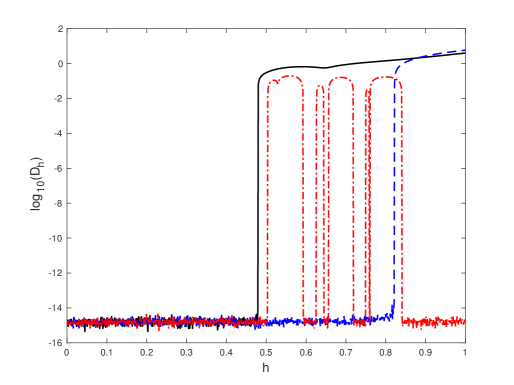
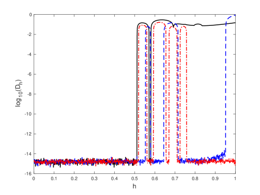
Figure 1: Absolute value of the largest eigenvalue of the approximations $S_{h}^{[3,1]}$ (black solid line), $S_{h}^{[3,2]}$ (red dash-dotted line) and $S_{h}^{[4]}$ (blue dashed line) for different values of $h$ when $H=A+B$ is a real symmetric matrix with simple eigenvalues. Left: $A$ and $B$ are also real symmetric. Right: $A$ and $B$ are real, but not symmetric.

Our next simulation concerns a real (but not symmetric) matrix $H$ with all its eigenvalues real and simple. Again, there exists a threshold $h^{*}>0$ such that for $h<h^{*}$ the schemes render unitary approximations. This is clearly visible in Figure 2 (left panel). If we consider instead a completely arbitrary real matrix $H$, then the outcome is rather different: $D_{h}>0$ for any $h>0$ (right panel; for this example $D_{h}=9.79\cdot 10^{-4}$ already for $h=0.001$).

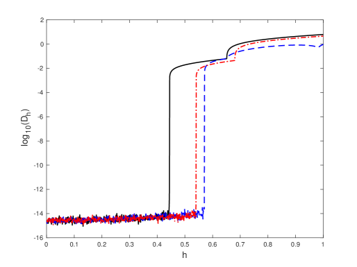
Figure 2: Same as Figure 1 when $H=A+B$ is a real (but not symmetric) matrix. Left: the eigenvalues of $H$ are real and simple. Right: the eigenvalues of $H$ are arbitrary.

Next we illustrate the situation when the real matrix $H$ has multiple eigenvalues but is still diagonalizable. As before, we consider first the analogue of Figure 1, namely: $H$ is symmetric, with $A$ and $B$ symmetric matrices (Figure 3, left panel) and $A$ and $B$ are real, but not symmetric (right panel). In the first case we notice that, whereas all the eigenvalues of the approximations rendered by $S_{h}^{[3,1]}$ and $S_{h}^{[4]}$ still have absolute value 1 for some interval $0<h<h^{*}$, this is clearly not the case of $S_{h}^{[3,2]}$. If, on the other hand, the splitting is done is such a way that $A$ and $B$ are not symmetric (but still real), then $D_{h}>0$ even for very small values of $h$. The same behavior is observed when $H$ is taken as a real (but not symmetric), diagonalizable matrix with multiple real eigenvalues.

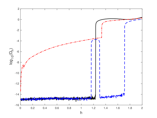
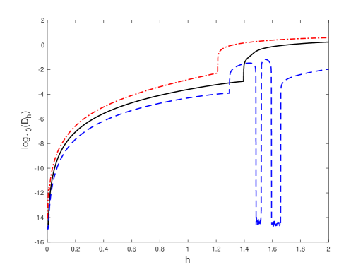
Figure 3: Same as Figure 1 when $H=A+B$ is a real symmetric matrix with multiple eigenvalues. Left: $A$ and $B$ are real symmetric matrices. Right: $A$ and $B$ are real, but not symmetric.

The different phenomena exhibited by these examples require then a detailed numerical analysis of the class of schemes involved, trying to explain in particular the role played by the eigenvalues of the matrix $H$ in the final outcome, as well as the different behavior of $S_{h}^{[3,1]}$ and $S_{h}^{[3,2]}$. This will be the subject of the next section.

3 Numerical analysis of reversible integration schemes

3.1 Main results

We next state two theorems and two additional corollaries that, generally speaking, justify the previous experiments and explain the good behavior exhibited by reversible methods.

Theorem 3.1

Let $H\in\mathbb{R}^{N\times N}$ be a real matrix and let $S_{h}\in\mathbb{C}^{N\times N}$ be a family of complex matrices depending smoothly on $h\in\mathbb{R}$ such that

• $S_{h}$ is a reversible map in the previous sense, so that

  $$\overline{S}_{h}=S_{h}^{-1};$$

• $S_{h}$ is consistent with $\exp(ihH)$, i.e. there exists $p\geq 1$ such that

  $$S_{h}\mathop{=}_{h\to 0}\mathrm{e}^{ihH}+\mathcal{O}(h^{p+1});$$ (3.1)

• the eigenvalues of $H$ are real and simple.

Then there exist

• $D_{h}$, a family of real diagonal matrices depending smoothly on $h$,

• $P_{h}$, a family of real invertible matrices depending smoothly on $h$,

such that $P_{h}=P_{0}+\mathcal{O}(h^{p})$, $D_{h}=D_{0}+\mathcal{O}(h^{p})$ and, provided that $|h|$ is small enough,

$$S_{h}=P_{h}\,\mathrm{e}^{ihD_{h}}\,P_{h}^{-1}.$$ (3.2)

Corollary 3.2

In the setting of Theorem 3.1, there exists a constant $C>0$ such that, provided that $|h|$ is small enough, for all $u\in\mathbb{C}^{N}$ and all eigenvalues $\omega\in\sigma(H)$, one has

$$\sup_{n\geq 0}\,\Big{|}|\Pi_{\omega}S_{h}^{n}u|-|\Pi_{\omega}u|\Big{|}\leq C|h|^{p}|u|,$$ (3.3)

where $\Pi_{\omega}$ denotes the spectral projector onto $\mathrm{Ker}(H-\omega I_{N})$. Moreover, if $H$ is symmetric, the norm and the energy are almost conserved, in the sense that, for all $u\in\mathbb{C}^{N}$, it holds that

$$\sup_{n\in\mathbb{Z}}\,\big{|}\mathcal{M}(S_{h}^{n}u)-\mathcal{M}(u)\big{|}\leq C|h|^{p}|u|^{2}\qquad\mathrm{and}\qquad\sup_{n\in\mathbb{Z}}\,\big{|}\mathcal{H}(S_{h}^{n}u)-\mathcal{H}(u)\big{|}\leq C|h|^{p}|u|^{2},$$ (3.4)

where $\mathcal{M}(u)=|u|^{2}$ and $\mathcal{H}(u)=\overline{u}^{T}Hu$.

Proof:[Proof of Corollary 3.2] First, we focus on (3.3). We note that by consistency, we have

$$D_{0}=P_{0}^{-1}HP_{0}.$$

Since the eigenvalues of $H$ are simple, it follows that the spectral projectors are all of the form

$$\Pi^{(j)}=P_{0}(e_{j}\otimes e_{j})P_{0}^{-1},$$ (3.5)

where $e_{1},\ldots,e_{N}$ denotes the canonical basis of $\mathbb{R}^{N}$. Then, we note that for all $n\in\mathbb{Z}$, we have

$$S_{h}^{n}=P_{h}\,\mathrm{e}^{inhD_{h}}\,P_{h}^{-1}.$$

Therefore, since $\mathrm{e}^{inhD_{h}}$ is uniformly bounded with respect to $h$ and $n$ (because $D_{h}$ is a real diagonal matrix) and $P_{h}=P_{0}+\mathcal{O}(h^{p})$, it follows that

$$S_{h}^{n}=P_{0}\,\mathrm{e}^{inhD_{h}}\,P_{0}^{-1}+\mathcal{O}(h^{p}),$$

where the implicit constant in $\mathcal{O}$ term does not depend on $n$ (here and later). Therefore, it is enough to use the explicit formula (3.5) to prove that

$$\Pi^{(j)}S_{h}^{n}=P_{0}(e_{j}\otimes e_{j})P_{0}^{-1}P_{0}\,\mathrm{e}^{inhD_{h}}P_{0}^{-1}+\mathcal{O}(h^{p})=\mathrm{e}^{inh(D_{h})_{j,j}}\Pi^{(j)}+\mathcal{O}(h^{p}).$$

As a consequence, the estimate (3.3) follows directly by the triangular inequality :

$$|\Pi^{(j)}S_{h}^{n}u|=|\mathrm{e}^{inh(D_{h})_{j,j}}\Pi^{(j)}u+\mathcal{O}(h^{p})(u)|\leq|\mathrm{e}^{inh(D_{h})_{j,j}}\Pi^{(j)}u|+|u|\mathcal{O}(h^{p})=|\Pi^{(j)}u|+|u|\mathcal{O}(h^{p}).$$

Now, we focus on (3.4). Here, since $H$ is assumed to be symmetric, its eigenspaces are orthogonal. Therefore by the Pythagorean theorem, we have

$$\mathcal{M}(u)=\sum_{\omega\in\sigma(H)}|\Pi_{\omega}(u)|^{2}\quad\mathrm{and}\quad\mathcal{H}(u)=\sum_{\omega\in\sigma(H)}\omega|\Pi_{\omega}(u)|^{2}.$$

As a consequence, (3.4) follows directly of (3.3). $\Box$

The main limitation of Theorem 3.1 is the assumption on the simplicity of the eigenvalues of $H$. Indeed, even if this assumption is typically satisfied, it depends only on the equation we aim at solving and not of the numerical method one uses. The following theorem, which is a refinement of Theorem 3.1, remedies this point by making an assumption on the leading term of the consistency error (which is typically satisfied for generic choices of numerical integrators).

Theorem 3.3

Let $H\in\mathbb{R}^{N\times N}$ be a real matrix and let $S_{h}\in\mathbb{C}^{N\times N}$ be a family of complex matrices depending smoothly on $h$ such that

• $S_{h}$ is a reversible map, i.e.

  $$\overline{S}_{h}=S_{h}^{-1};$$

• $S_{h}$ is consistent with $\exp(ihH)$, i.e.

  $$S_{h}\mathop{=}_{h\to 0}\mathrm{e}^{ihH}+ih^{p+1}R+\mathcal{O}(h^{p+2}),$$ (3.6)

  where $p\geq 1$ is the order of consistency and $R$ is a real matrix;

• $H$ is diagonalizable and its eigenvalues are real;

• for all $\omega\in\sigma(H)$, the eigenvalues of $\Pi_{\omega}R_{|E_{\omega}(H)}$ are real and simple, where $\Pi_{\omega}$ denotes the spectral projector on $E_{\omega}(H):=\mathrm{Ker}(H-\omega I_{N})$.

Then there exist

• $D_{h}$, a family of real diagonal matrices depending smoothly on $h$,

• $P_{h}$, a family of real invertible matrices depending smoothly on $h$,

such that, both $P_{0}^{-1}BP_{0}$ and $P_{0}^{-1}HP_{0}$ are diagonal, where $B:=\sum_{\omega\in\sigma(H)}\Pi_{\omega}\,R\,\Pi_{\omega}$, and provided that $|h|$ is small enough, it holds that

$$S_{h}=P_{h}\,\mathrm{e}^{ihD_{h}}\,P_{h}^{-1}.$$ (3.7)

Corollary 3.4

In the setting of Theorem 3.3, there exists a constant $C>0$ such that, provided that $|h|$ is small enough, for all $u\in\mathbb{C}^{N}$, all $\omega\in\sigma(H)$ and all $\lambda\in\sigma(\Pi_{\omega}R_{|E_{\omega}(H)})$, we have

$$\sup_{n\geq 0}\,\Big{|}|\mathcal{P}_{\lambda,\omega}S_{h}^{n}u|-|\mathcal{P}_{\lambda,\omega}u|\Big{|}\leq C|h||u|,$$

where $\mathcal{P}_{\lambda,\omega}$ denotes the projector along $\bigoplus_{(\eta,\mu)\neq(\lambda,\omega)}E_{\eta}(\Pi_{\mu}R_{|E_{\mu}(H)})$ onto $E_{\lambda}(\Pi_{\omega}R_{|E_{\omega}(H)})$.

Moreover, if $H$ and $R$ are symmetric, for all $\omega\in\sigma(H)$, one gets

$$\sup_{n\geq 0}\,\Big{|}|\Pi_{\omega}S_{h}^{n}u|^{2}-|\Pi_{\omega}u|^{2}\Big{|}\leq C|h||u|^{2},$$

and the mass and the energy are almost conserved, i.e. for all $u\in\mathbb{C}^{N}$, it holds that

$$\sup_{n\in\mathbb{Z}}\,\big{|}\mathcal{M}(S_{h}^{n}u)-\mathcal{M}(u)\big{|}\leq C|h||u|^{2}\qquad\mathrm{and}\qquad\sup_{n\in\mathbb{Z}}\,\big{|}\mathcal{H}(S_{h}^{n}u)-\mathcal{H}(u)\big{|}\leq C|h||u|^{2},$$

where, as before, $\mathcal{M}(u)=|u|^{2}$ and $\mathcal{H}(u)=\overline{u}^{T}Hu$.

Proof:[Proof of Corollary 3.4] The proof is almost identical to the one of Corollary 3.2. The key point is that, since both $P_{0}^{-1}BP_{0}$ and $P_{0}^{-1}HP_{0}$ are diagonal, then the projectors $\mathcal{P}_{\lambda,\omega}$ are exactly the projectors $\Pi^{(j)}$, $1\leq j\leq N$ (given by (3.5)). Note that, contrary to Theorem 3.1, in Theorem 3.3 one does not claim that $P_{h}=P_{0}+\mathcal{O}(h^{p})$. A priori, here, in general, the best estimate we expect is $P_{h}=P_{0}+\mathcal{O}(h)$ (which follows directly from the smoothness of $P_{h}$ with respect to $h$). It is this loss which explains why, in Corollary 3.4, the error terms are of order $\mathcal{O}(h)$ whereas they are of order $\mathcal{O}(h^{p})$ in Corollary 3.2. $\Box$

Remark.

Before starting the proof of these theorems, let us provide some comments about the context and the ideas involved.

• In Theorem 3.1 and its proof, we are just putting $S_{h}$ in Birkhoff normal form. The fact that $S_{h}$ can be diagonalized is due to the simplicity of the eigenvalues of $H$ while the fact that its eigenvalues are complex numbers of modulus $1$ is due the reversibility of $S_{h}$. This approach is robust and well known, in particular it can be extended to the nonlinear setting (see e.g. [12, section V.1]). Note that here, we reach convergence of the Birkhoff normal form because the system is linear.

• Theorem 3.3 is a refinement of Theorem 3.1. To prove the absence of resonances due to the multiplicity of the eigenvalues of $H$, we use the first correction to the frequencies generated by the perturbation of $H$ (i.e., the projections of $R$ in Theorem 3.3). This approach is typical of what one does in the proof of Nekhoroshev theorems or KAM theorems (see also [12]).

• In order to give some intuition about the proof and the assumptions of Theorem 3.1, let us prove simply that, provided $h$ is small enough, $S_{h}$ is conjugated to a unitary matrix. Indeed, since $S_{h}$ is reversible it writes as

  $$S_{h}=e^{ihH_{h}},$$

  where $H_{h}=H+\mathcal{O}(h^{p})$ is a real matrix (provided that $h$ is small enough). Now, since the set of the real matrices whose eigenvalues are simple and real is open in the space of the real matrices (by continuity of the eigenvalues) and $H_{h}$ is a real perturbation of such a matrix ($H$ by assumption), we deduce that, provided $h$ is small enough, its eigenvalues are simple and real. This implies that $H_{h}$ is conjugated to a real diagonal matrix and so that $S_{h}$ is conjugated to a unitary matrix.

3.2 Technical lemmas

In the proof of the previous theorems we will make use of the following three lemmas.

Lemma 3.5

Let $M$ be a complex matrix and let $P$ be a complex invertible matrix. Then $\mathrm{ad}_{P^{-1}MP}$ and $\mathrm{ad}_{M}$ are similar. More precisely,

$$\mathrm{ad}_{\mathrm{int}_{P}\,M}=(\mathrm{int}_{P})\mathrm{ad}_{M}(\mathrm{int}_{P})^{-1},$$

where $\mathrm{int}_{P}M:=P^{-1}MP$. Here $\mathrm{ad}_{M}$ stands for the adjoint operator: $\mathrm{ad}_{M}X:=[M,X]=MX-XM$, for any matrix $X$.

Proof: A straightforward calculation shows that, for any $X$,

$$(\mathrm{int}_{P})\mathrm{ad}_{M}X=P^{-1}[M,X]P=[P^{-1}MP,P^{-1}XP]=\mathrm{ad}_{\mathrm{int}_{P}\,M}(P^{-1}XP)=\mathrm{ad}_{\mathrm{int}_{P}\,M}(\mathrm{int}_{P})X.$$

$\Box$

Lemma 3.6

Let $M$ be a complex matrix. Then $M$ is diagonalizable if and only if the kernel and the image of $\mathrm{ad}_{M}$ are supplementary, i.e.

$$\mathrm{Ker}_{\mathbb{C}}\ \mathrm{ad}_{M}\cap\mathrm{Im}_{\mathbb{C}}\ \mathrm{ad}_{M}=\{0\}.$$ (3.8)

Proof: We can assume, in virtue of Lemma 3.5 and without loss of generality, that $M$ is in Jordan normal form. On the one hand, if $M$ is diagonal, we have $\mathrm{ad}_{M}A=((m_{i,i}-m_{j,j})A)_{i,j}$ and so the support of the matrices in $\mathrm{Ker}_{\mathbb{C}}\ \mathrm{ad}_{M}$ and $\mathrm{Im}_{\mathbb{C}}\ \mathrm{ad}_{M}$ are clearly disjoint (which implies (3.8)). Conversely, doing calculations by blocks it is enough to consider the case where $M=\lambda I_{N}+\mathcal{N}$ is a Jordan matrix (i.e. $\lambda\in\mathbb{C}$ and $\mathcal{N}$ nilpotent). Then we just have to note that $\mathrm{ad}_{\lambda I_{N}+\mathcal{N}}=\mathrm{ad}_{\mathcal{N}}$ and that since $\mathrm{ad}_{\mathcal{N}}$ is nilpotent necessarily we have $\mathrm{Ker}_{\mathbb{C}}\ \mathrm{ad}_{\mathcal{N}}\cap\mathrm{Im}_{\mathbb{C}}\ \mathrm{ad}_{\mathcal{N}}\neq\{0\}$. $\Box$

Lemma 3.7

Let $M_{h}$ be a family of real matrices depending smoothly on $h$ and of the form

$$M_{h}=M_{0}+\mathcal{O}(h^{p}),\quad\mbox{ where }\quad p\geq 1.$$

If $M_{0}$ is diagonalizable on $\mathbb{C}$, then there exists a family of real matrices $\chi_{h}$, depending smoothly on $h$, such that if $|h|$ is small enough, $\mathrm{e}^{-h^{p}\chi_{h}}M_{h}\,\mathrm{e}^{h^{p}\chi_{h}}$ commutes with $M_{0}$, i.e.

$$[\mathrm{e}^{h^{p}\chi_{h}}M_{h}\,\mathrm{e}^{-h^{p}\chi_{h}},M_{0}]=0.$$

Proof: We aim at designing the family $\chi_{h}$ as solution of the equation

$$\mathrm{ad}_{M_{0}}\left(\mathrm{e}^{h^{p}\chi_{h}}M_{h}\,\mathrm{e}^{-h^{p}\chi_{h}}\right)=0.$$

Thanks to the well known identity $\mathrm{e}^{A}B\,\mathrm{e}^{-A}=\mathrm{e}^{\mathrm{ad}_{A}}B$, this equation rewrites as

$$\mathrm{ad}_{M_{0}}\left(\mathrm{e}^{h^{p}\mathrm{ad}_{\chi_{h}}}M_{h}\right)=0.$$ (3.9)

Next we write the Taylor expansion of $M_{h}$ at order $p$ as

$$M_{h}=M_{0}+h^{p}R_{h},$$

where $R_{h}$ is a family of real matrices depending smoothly on $h$. Then, isolating the terms of order $0$ (and dividing by $h^{p}$), the equation (3.9) leads to

$$f(h,\chi_{h}):=\mathrm{ad}_{M_{0}}\left(\mathrm{e}^{h^{p}\mathrm{ad}_{\chi_{h}}}R_{h}-\varphi_{1}(h^{p}\mathrm{ad}_{\chi_{t}})\,\mathrm{ad}_{M_{0}}\chi_{h}\right)=0,$$

where $\varphi_{1}(z):=\frac{e^{z}-1}{z}$. We restrict ourselves to $\chi_{h}$ in $\mathrm{Im}_{\mathbb{R}}\,\mathrm{ad}_{M_{0}}$ and consider $f$ as a smooth map from $\mathbb{R}\times\mathrm{Im}_{\mathbb{R}}\,\mathrm{ad}_{M_{0}}$ to $\mathrm{Im}_{\mathbb{R}}\,\mathrm{ad}_{M_{0}}$. To solve the equation $f(h,\chi_{h})=0$ using the implicit function theorem, we just have to design $\chi_{0}$ so that

$$f(0,\chi_{0})=\mathrm{ad}_{M_{0}}R_{0}-\mathrm{ad}_{M_{0}}\chi_{0}=0$$

and prove that $\mathrm{d}_{\chi}f(0,\chi_{0})=-\mathrm{ad}_{M_{0}}:\mathrm{Im}_{\mathbb{R}}\,\mathrm{ad}_{M_{0}}\to\mathrm{Im}_{\mathbb{R}}\,\mathrm{ad}_{M_{0}}$ is invertible. Actually, these properties are clear because the first one is a consequence of the second one, whereas the second follows directly from Lemma 3.6. $\Box$

3.3 Proofs of the theorems

We are now in a position to prove Theorems 3.1 and 3.3. Without loss of generality, and to simplify notations, we assume that $H$ is diagonal

$$H=\begin{pmatrix}\omega_{1}I_{n_{1}}\\ &\ddots\\ &&\omega_{d}I_{n_{d}}\end{pmatrix},$$

where $\omega_{1}<\cdots<\omega_{d}$ denote the eigenvalues of $H$ and $n_{1},\cdots,n_{d}$ are positive integers satisfying $n_{1}+\cdots+n_{d}=N$.

Thanks to the consistency assumption (3.6) (which is equivalent to (3.1)), provided that $|h|$ is small enough, $S_{h}$ rewrites as

$$S_{h}=\mathrm{e}^{ihH_{h}},\quad\mbox{ where }\quad H_{h}=H+h^{p}R+\mathcal{O}(h^{p+1}).$$

Moreover, the reversibility assumption $S_{h}^{-1}=\overline{S}_{h}$ implies that $H_{h}$ is a real matrix (provided that $|h|$ is small enough). Note that, hence, we deduce that $R$ is also a real matrix. Then, applying Lemma 3.7 to $H_{h}$, we get a family of real matrices $\chi_{h}$ such that, provided that $|h|$ is small enough,

$$[W_{h},H]=0,\qquad\mbox{ where }\qquad W_{h}=\mathrm{e}^{h^{p}\chi_{h}}H_{h}\,\mathrm{e}^{-h^{p}\chi_{h}}.$$

We conclude that $W_{h}$ is block-diagonal (with the same structure of blocks as $H$), i.e. there exists some $n_{j}\times n_{j}$ real matrices $W_{h}^{(j)}$ such that

$$W_{h}=\begin{pmatrix}W_{h}^{(1)}\\ &\ddots\\ &&W_{h}^{(d)}\end{pmatrix}.$$ (3.10)

As a consequence, if the eigenvalues of $H$ are simple (i.e. $d=N$ and $n_{j}=1$ for all $j$) then $W_{h}$ is diagonal. Therefore, in this case, it is enough to set $P_{h}=\mathrm{e}^{-h^{p}\chi_{h}}$ and $W_{h}=D_{h}$ to conclude the proof of Theorem 3.1.

So, from now on, we only focus on the proof of Theorem 3.3. First, we aim at identifying the matrices on the blocks in (3.10). The Taylor expansion of $W_{h}$ is clearly

$$W_{h}=H+h^{p}B+\mathcal{O}(h^{p+1}),\qquad\mbox{ with }\qquad B:=R+[\chi_{0},H].$$

However, since $[W_{h},H]=0$, we deduce that $[B,H]=0$ and so that $B$ is block-diagonal. Moreover, since the matrix $[\chi_{0},H]$ is identically equal to zero on the diagonal blocks, the diagonal blocks of $B$ are exactly those of $R$. As a consequence, with a slight abuse of notations, we may write

$$W_{h}^{(j)}=\omega I_{n_{j}}+h^{p}B^{(j)}+h^{p+1}Y_{h}^{(j)},\qquad\mbox{ where }\qquad B^{(j)}:=\Pi_{\omega_{j}}R_{|E_{\omega_{j}}(H)}$$

and $Y_{h}^{(j)}$ is a family of real matrices depending smoothly on $h$.

Next we aim at diagonalizing these blocks. By assumption, the eigenvalues of each matrix $B^{(j)}$ are real and simple. Therefore, all $B^{(j)}$ are diagonalizable. As a consequence, and again by applying Lemma 3.7, we get a family of real matrices $\Upsilon^{(j)}_{h}$ such that if $|h|$ is small enough, for all $j\in\llbracket 1,d\rrbracket$ we have

$$\Big{[}\mathrm{e}^{h\Upsilon^{(j)}_{h}}(B^{(j)}+hY_{h}^{(j)})\mathrm{e}^{-h\Upsilon^{(j)}_{h}},B^{(j)}\Big{]}=0.$$

This means that the eigenspaces of $B^{(j)}$ are stable by the action of $\mathrm{e}^{h\Upsilon^{(j)}_{h}}(B^{(j)}+hY_{h}^{(j)})\mathrm{e}^{-h\Upsilon^{(j)}_{h}}$. However, by assumption, these spaces are lines. Therefore, if $Q^{(j)}$ is a real invertible matrix such that $Q^{(j)}B^{(j)}(Q^{(j)})^{-1}$ is diagonal then $Q^{(j)}\mathrm{e}^{h\Upsilon^{(j)}_{h}}(B^{(j)}+hY_{h}^{(j)})\mathrm{e}^{-h\Upsilon^{(j)}_{h}}(Q^{(j)})^{-1}$ is also diagonal.

Finally, as a consequence, setting

$$P_{h}:=\mathrm{e}^{-h^{p}\chi_{h}}\begin{pmatrix}\mathrm{e}^{-h\Upsilon^{(1)}_{h}}Q^{(1)}\\ &\ddots\\ &&\mathrm{e}^{-h\Upsilon^{(d)}_{h}}Q^{(d)}\end{pmatrix}$$

we have proven that $D_{h}:=P_{h}^{-1}H_{h}P_{h}$ is real diagonal, which concludes the proof of Theorem 3.3.

3.4 Applications to reversible splitting and composition methods

Theorems 3.1 and 3.3 shed light on the behavior observed in the examples collected in Section 2. Thus, suppose $H=A+B$ is a real symmetric matrix, with $A$, $B$ also real. Furthermore, consider a splitting scheme $S_{h}$ of the form (1.2) with coefficients satisfying the symmetry conditions (1.3) and consistency,

$$a_{0}+\cdots+a_{2n}=1,\qquad\qquad b_{0}+\cdots+b_{2n-1}=1.$$

Clearly, $S_{h}$ is a reversible map and moreover, it is consistent with $\mathrm{e}^{ihH}$ at least at order $1$, so that (3.1) holds with $p\geq 1$. Since $H$ is real symmetric, it is diagonalizable. Therefore, if the eigenvalues of $H$ are simple, the dynamics of $(S_{h}^{n})_{n\in\mathbb{Z}}$ is given by Theorem 3.1: for sufficiently small $h$, there exist real matrices $D_{h}$ (diagonal) and $P_{h}$ (invertible) so that $S_{h}^{n}=P_{h}\,\mathrm{e}^{inD_{h}}P_{h}^{-1}$, all the eigenvalues of $S_{h}$ verify $|\omega_{j}|=1$ and $\mathcal{M}(u)$ and $\mathcal{H}(u)$ are almost preserved for long times. This corresponds to the examples of Figure 1. The same conclusions apply as long as $H$ is a real matrix with all its eigenvalues real and simple (Figure 2, left), whereas the general case of complex eigenvalues is not covered by the theorem, and no preservation is ensured (Figure 2, right).

Suppose now that the real matrix $H$ has multiple real eigenvalues, but is still diagonalizable, and that $A$ and $B$ are real and symmetric. In that case, a symmetric-conjugate splitting method satisfy both conditions (1.4) and (1.5), so that it can be written as

$$S_{h}=e^{ihH_{h}},$$

where $H_{h}$ is a family of real matrices whose even terms in $h$ are symmetric and odd terms are skew-symmetric. Suppose in addition that $S_{h}$ is of even order (i.e., $p$ is even in (3.6)). In that case the matrix $R$ in Theorem 3.3 is symmetric, and so its eigenvalues are real. Moreover, since $R$ strongly depends on the coefficients $a_{j},b_{j}$ and the decomposition $H=A+B$, it is very likely that typically the eigenvalues of the operators $\Pi_{\omega}R_{|E_{\omega}(H)}$ are simple and so that the dynamics of $(S_{h}^{n})_{n\in\mathbb{Z}}$ is given by Theorem 3.3 and is therefore similar to the one of $(\mathrm{e}^{inhH})_{n\in\mathbb{Z}}$. Notice that this does not necessarily hold if the scheme is of odd order and/or $A$ and $B$ are not symmetric. This phenomenon is clearly illustrated in the examples of Figure 3 by methods $S_{h}^{[3,2]}$ and $S_{h}^{[4]}$.

Notice, however, that method $S_{h}^{[3,1]}$, although of odd order, works in fact better than expected from the previous considerations. The reason for this behavior resides in the following

Proposition 3.8

The 3th-order symmetric-conjugate splitting method

$$S_{h}^{[3,1]}=\mathrm{e}^{ih\overline{b}_{0}B}\,\mathrm{e}^{ih\overline{a}_{1}A}\,\mathrm{e}^{ihb_{1}B}\,\mathrm{e}^{iha_{1}A}\,\mathrm{e}^{ihb_{0}B},$$

with $a_{1}=\frac{1}{2}+i\frac{\sqrt{3}}{6}$, $b_{0}=\frac{a_{1}}{2}$, $b_{1}=\frac{1}{2}$, is indeed conjugate to a reversible integrator $V_{h}$ of order 4, i.e., there exists a real near-identity transformation $F_{h}$ such that $F_{h}\,S_{h}^{[3,1]}\,F_{h}^{-1}=V_{h}=\mathrm{e}^{ihH}+\mathcal{O}(h^{5})$ and $\overline{V}_{h}=V_{h}^{-1}$.

Proof: Method $S_{h}^{[3,1]}$ constitutes in fact a particular case of a composition $\psi_{h}=\mathcal{S}_{\bar{\alpha}h}^{[2]}\,\mathcal{S}_{\alpha h}^{[2]}$, where $\mathcal{S}_{h}^{[2]}$ is a time-symmetric 2nd-order method and $\alpha=a_{1}$. Specifically, $S_{h}^{[3,1]}$ is recovered when $\mathcal{S}_{h}^{[2]}=\mathrm{e}^{\frac{h}{2}B}\,\mathrm{e}^{hA}\,\mathrm{e}^{\frac{h}{2}B}$. Therefore, it can be written as

$$\mathcal{S}_{h}^{[2]}=\exp(ihH-ih^{3}F_{3}+ih^{5}F_{5}+\cdots)$$

for certain real matrices $F_{2j+1}$. In consequence, by applying the BCH formula, one gets $\psi_{h}=\mathrm{e}^{W(h)}$, with

$$W(h)=ihH+\frac{1}{2}h^{4}|\alpha|^{2}(\alpha^{2}-\bar{\alpha}^{2})[H,F_{3}]+ih^{5}\big{(}w_{5,1}F_{5}+w_{5,2}[H,[H,F_{3}]]\big{)}+\mathcal{O}(h^{6}).$$

Here $w_{5,j}$ are polynomials in $\alpha$. Now let us consider

$$V_{h}=\mathrm{e}^{V(h)}=\mathrm{e}^{\lambda h^{3}F_{3}}\,\mathrm{e}^{W(h)}\,\mathrm{e}^{-\lambda h^{3}F_{3}}$$

for a given parameter $\lambda$. Then, clearly,

$$V(h)=\mathrm{e}^{\lambda h^{3}\mathrm{ad}_{F_{3}}}W(h)=ihH+h^{4}\left(\frac{1}{2}\alpha^{3}-i\lambda\right)[H,F_{3}]+\mathcal{O}(h^{5}),$$

so that by choosing $\lambda=-\frac{i}{2}\alpha^{3}=-\frac{\sqrt{3}}{18}$, we have $V(h)=ihH+\mathcal{O}(h^{5})$ and the stated result is obtained, with $F_{h}=\mathrm{e}^{\lambda h^{3}F_{3}}$. $\Box$

This result can be generalized as follows: given a time-symmetric method $\mathcal{S}_{h}^{[2k]}$ of order $2k$, if $\alpha$ is chosen so that the composition $\psi_{h}=\mathcal{S}_{\bar{\alpha}h}^{[2k]}\,\mathcal{S}_{\alpha h}^{[2k]}$ is of order $2k+1$, then $\psi_{h}$ is conjugate to a reversible method of order $2k+2$.

Theorems 3.1 and 3.3 also allow one to explain the good behavior shown by symmetric-conjugate composition methods for this type of problems. In fact, suppose $H$ is a real symmetric matrix and $\Phi_{H}^{z}$ is a family of linear maps which are consistent with $\mathrm{e}^{izH}$ at least at order $1$ and satisfy

$$(\Phi_{H}^{z})^{-1}=\overline{\Phi_{H}^{\overline{z}}}.$$

If we define $S_{h}$ as the symmetric-conjugate composition

$$S_{h}=\Phi_{H}^{\alpha_{0}h}\cdots\Phi_{H}^{\alpha_{n}h},$$

where $\alpha_{j}$ are some complex coefficients satisfying the symmetry condition

$$\alpha_{n-j}=\overline{\alpha}_{j},\qquad j=1,2,\ldots$$

and the consistency condition

$$\alpha_{0}+\cdots+\alpha_{n}=1,$$

then $S_{h}$ is a reversible map. Moreover, it is consistent with $\mathrm{e}^{ihH}$ at least at order $1$. Therefore, one can apply Theorem 3.1 and Theorem 3.3 also in this case. Notice, in particular, that even if the maps $\mathrm{e}^{iha_{j}A}$ and/or $\mathrm{e}^{ihb_{j}B}$ in the symmetric-conjugate splitting method (1.2) are not computed exactly, but only conveniently approximated (for instance, by the midpoint rule), the previous theorems still apply, so that one can expect good long term behavior from the resulting approximation.

4 Symmetric-conjugate splitting methods for the Schrödinger equation

An important application of the previous results corresponds to the numerical integration of the time dependent Schrödinger equation ($\hbar=m=1$)

$$i\frac{\partial}{\partial t}\psi(x,t)=\hat{H}\psi(x,t),\qquad\quad\psi(x,0)=\psi_{0}(x),$$ (4.1)

where $\psi:\mathbb{R}^{3}\times\mathbb{R}\longrightarrow\mathbb{C}$. The Hamiltonian operator $\hat{H}$ is the sum $\hat{H}=\hat{T}+\hat{V}$ of the kinetic energy operator $\hat{T}$ and the potential $\hat{V}$. Specifically,

$$(\hat{T}\psi)(x)=-\frac{1}{2}\Delta\psi(x,t),\qquad\quad(\hat{V}\psi)(x)=\hat{V}(x)\psi(x,t).$$

In addition, a simple computation shows that $[\hat{V},[\hat{T},\hat{V}]]\ \psi=|\nabla\hat{V}|^{2}\psi$, and therefore

$$[\hat{V},[\hat{V},[\hat{V},\hat{T}]]]\ \psi=0.$$ (4.2)

Assuming $d=1$ and periodic boundary conditions, the application of a pseudo-spectral method in space (with $N$ points) leads to the $N$-dimensional system (1.1), where $u(0)=u_{0}\in\mathbb{C}^{N}$ and $H$ represents the (real symmetric) $N\times N$ matrix associated with the operator $-\hat{H}$ [16]. Now

$$H=A+B,$$

where $A$ is the (minus) differentiation matrix corresponding to the discretization of $\hat{T}$ (a real and symmetric matrix) and $B$ is the diagonal matrix associated to $-\hat{V}$ at the grid points. Since $\exp(tA)$ can be efficiently computed with the fast Fourier transform (FFT) algorithm, it is a common practice to use splitting methods of the form (1.2) to integrate this problem. In this respect, notice that property (4.2) will be inherited by the matrices $A$ and $B$ only if the number of discretization points $N$ is sufficiently large to achieve spectral accuracy, i.e.,

$$[B,[B,[B,A]]]u=0\qquad\mbox{ if $N$ is large enough. }$$ (4.3)

Assuming this is satisfied, then there is a reduction in the number of conditions necessary to construct a method (1.2) of a given order $p$ [12, 2]. Integrators of this class are sometimes called Runge–Kutta–Nyström (RKN) splitting methods [5].

Two further points are worth remarking. First, the computational cost of evaluating (1.2) is not significantly increased by incorporating complex coefficients into the scheme, since one has to use complex arithmetic anyway. Second, since $\sum_{j}a_{j}=1$ for a consistent method, if $a_{j}\in\mathbb{C}$, then both positive and negative imaginary parts are present, and this can lead to severe instabilities due to the unboundedness of the Laplace operator [8, 14]. On the other hand, the spurious effects introduced by complex $b_{j}$ can be eliminated (at least for sufficiently small values of $h$) by introducing an artificial cut-off bound in the potential when necessary.

In view of these considerations, we next limit our exploration to symmetric-conjugate splitting methods of the form (1.2) with $0<a_{j}<1$ and $b_{j}\in\mathbb{C}$ with $\Re(b_{j})>0$ to try to reduce the size of the error terms appearing in the asymptotic expansion of the modified Hamiltonian $H_{h}$ associated with the integrator.

For simplicity, we denote the symmetric-conjugate splitting schemes $S_{h}$ by their sequence of coefficients as

$$(a_{0},b_{0},a_{1},b_{1},\ldots,a_{r},b_{r},a_{r},\ldots,\overline{b}_{1},a_{1},\overline{b}_{0},a_{0}).$$ (4.4)

As a matter of fact, since $A$ and $B$ are sought to verify (4.3), sequences starting with $B$ may lead to schemes with a different efficiency, so that we also analyze methods of the form

$$(b_{0},a_{0},b_{1},a_{1},\ldots,b_{r},a_{r},\overline{b}_{r},\ldots,a_{1},\overline{b}_{1},a_{0},\overline{b}_{0}).$$ (4.5)

Schemes (4.4) and (4.5) include integrators where the central exponential corresponds to $A$ (when $b_{r}=0$) and $B$ (when $a_{r}=0$), respectively. The method has $s$ stages if the number of exponentials of $A$ is precisely $s$ for the scheme (4.5) or $s+1$ for the scheme (4.4).

The construction process of methods within this class is detailed elsewhere (e.g. [7, 5] and references therein), so that it is only summarized here. First, we get the order conditions a symmetric-conjugate scheme has to satisfy to achieve a given order $p=4,5$ and 6. These are polynomial equations depending on the coefficients $a_{j}$, $b_{j}$, and can be obtained by identifying a basis in the Lie algebra generated by $\{A,B\}$ and using repeatedly the BCH formula to express the splitting method as $S_{h}=\exp(hH_{h})$, with $H_{h}$ in terms of $A$, $B$ and their nested commutators. The order conditions up to order $p$ are obtained by requiring that $H_{h}=H+\mathcal{O}(h)^{p+1}$, and the number is 7, 11 and 16 for orders 4, 5 and 6, respectively.

Second, we take compositions (4.4) and (4.5) involving the minimum number of stages required to solve the order conditions and get eventually all possible solutions with the appropriate symmetry. Sometimes, one has to add parameters, because there are no such solutions. In particular, there are no 4th-order schemes with 4 stages with both $a_{j}>0$ and $\Re(b_{j})>0$.

Even when there are appropriate solutions, it may be convenient to explore compositions with additional stages to have free parameters for optimization. This strategy usually pays off when purely real coefficients are involved, and so it is worth to be explored also in this context. Of course, some optimization criterion related with the error terms and the computational effort has to be adopted. In our study we look at the error terms in the expansion of $H_{h}$ at successive orders and the size of the $b_{j}$ coefficients. Specifically, we compute for each method of order, say, $p$, the quantities

$$\Delta_{b}:=\sum_{j}|b_{j}|\qquad\mbox{ and }\qquad E_{f}^{(r+1)}:=s\,\big{(}\mathcal{E}_{r+1}\big{)}^{1/r},\qquad r=p,p+1,\ldots$$ (4.6)

Here $s$ is the number of stages and $\mathcal{E}_{r+1}$ is the Euclidean norm of the vector of error coefficients in $H_{h}$ at higher orders than the method itself. In particular, for a method of order $6$, $E_{f}^{(7)}$ gives an estimate of the efficiency of the scheme by considering only the error at order 7. By computing $E_{f}^{(8)}$ and $E_{f}^{(9)}$ for this method we get an idea of how the higher order error terms behave. It will be of interest, of course, to reduce these quantities as much as possible to get efficient schemes.

Solving the polynomial equations required to construct splitting methods with additional stages is not a trivial task, especially for orders 5 and 6. In these cases we have used the Python function fsolve of the SciPy library, with a large number of initial points in the space of parameters to start the procedure. From the total number of valid solutions thus obtained, we have selected those leading to reasonably small values of all quantities (4.6) and checked them on numerical examples.

The corresponding values for the most efficient methods we have found by following this approach have been collected in Table 1, where $\mathcal{NA}_{s}^{*[p]}$ refers to a symmetric-conjugate method of type (4.4) of order $p$ involving $s$ stages, and $\mathcal{NB}_{s}^{*[p]}$ is a similar scheme of type (4.5). For completeness, we have also included the most efficient integrators of order 4, 6 and 8 with real coefficients for systems satisfying the condition (4.3) (same notation without $*$) and also the symmetric-conjugate splitting schemes presented in [10, 11] (denoted by $\mathcal{GB}_{s}^{*[p]}$). They do not take into account the property (4.3) for their formulation.

In Table 1 we also write the value of $\Delta_{a}:=\sum_{j}|a_{j}|$ and $\Delta_{b}:=\sum_{j}|b_{j}|$ for each method. Of course, by construction, $\Delta_{a}=1$ for all symmetric-conjugate integrators. The coefficients of the most efficient schemes we have found (in boldface) are collected in Table 2.

	$\Delta_{a}$	$\Delta_{b}$	$E_{f}^{(5)}$	$E_{f}^{(6)}$	$E_{f}^{(7)}$	$E_{f}^{(8)}$	$E_{f}^{(9)}$
$\mathcal{NA}_{6}^{*[4]}$	1.000	1.267	0.400	0.821	0.704	1.082	1.012
$\boldsymbol{\mathcal{NB}_{5}^{*[4]}}$	1.000	1.141	0.352	0.698	0.559	0.913	0.789
$\boldsymbol{\mathcal{NB}_{6}^{*[4]}}$	1.000	1.416	0.322	0.766	0.666	1.025	0.866
$\mathcal{NA}_{7}^{*[5]}$	1.000	1.662	–	0.695	0.817	1.013	1.132
$\mathcal{NA}_{8}^{*[5]}$	1.000	1.393	–	0.546	0.947	0.953	1.339
$\mathcal{NA}_{9}^{*[5]}$	1.000	1.456	–	0.498	0.970	1.157	1.357
$\mathcal{NB}_{7}^{*[5]}$	1.000	3.196	–	0.833	0.970	1.143	1.300
$\boldsymbol{\mathcal{NB}_{8}^{*[5]}}$	1.000	1.482	–	0.478	0.670	1.046	1.031
$\boldsymbol{\mathcal{NB}_{9}^{*[5]}}$	1.000	1.618	–	0.403	0.966	1.331	1.499
$\mathcal{NA}_{10}^{*[6]}$	1.000	1.528	–	–	0.906	1.204	1.298
$\boldsymbol{\mathcal{NA}_{11}^{*[6]}}$	1.000	2.092	–	–	0.656	1.418	1.643
$\mathcal{NB}_{10}^{*[6]}$	1.000	1.516	–	–	1.000	1.212	1.557
$\boldsymbol{\mathcal{NB}_{11}^{*[6]}}$	1.000	1.595	–	–	0.646	1.387	1.394
$\mathcal{GB}_{5}^{*[4]}$	1.000	1.133	0.477	0.662	0.662	0.885	0.807
$\mathcal{GB}_{9}^{*[5]}$	1.000	1.463	–	0.603	0.786	1.036	1.278
$\mathcal{GB}_{15}^{*[6]}$	1.000	1.692	–	–	1.515	1.434	2.169
$\mathcal{NB}_{6}^{[4]}$	2.401	1.156	0.291	–	0.809	–	1.307
$\mathcal{NB}_{11}^{[6]}$	2.494	1.206	–	–	0.784	–	1.664
$\mathcal{NA}_{14}^{[6]}$	1.659	2.012	–	–	0.627	–	2.238

Table 1: 1-norm and effective errors for several splitting methods of order 4, 5 and 6 designed for problems satisfying the condition (4.3).

	$a_{i}$	$b_{i}$
$\mathcal{NB}_{5}^{*[4]}$	$a_{0}=0.17354158169943656$	$b_{0}=0.06421454120274125+0.0245540186592381\,i$
	$a_{1}=0.19379086394173623$	$b_{1}=0.20166370500451958-0.0982277975564409\,i$
	$a_{2}=1-2\sum_{i=0}^{1}a_{i}$	$b_{2}=\frac{1}{2}-\sum_{i=0}^{1}\Re(b_{i})+0.1491719824749133\,i$
$\mathcal{NB}_{6}^{*[4]}$	$a_{0}=\frac{1}{5}$	$b_{0}=\frac{7}{100}+0.019444288930263294\,i$
	$a_{1}=0.054855282174763084$	$b_{1}=0.16-0.20579973912385285\,i$
	$a_{2}=\frac{1}{2}-\sum_{i=0}^{1}a_{i}$	$b_{2}=0.16251793145097668+0.21219211957584155\,i$
		$b_{3}=1-2\sum_{i=0}^{1}\Re(b_{i})$
$\mathcal{NB}_{8}^{*[5]}$	$a_{0}=0.13556579817637690$	$b_{0}=0.048-0.0045117121645322032\,i$
	$a_{1}=0.12110548685533656$	$b_{1}=0.159+0.039915395925895825\,i$
	$a_{2}=0.040926280383255811$	$b_{2}=0.08808186616153123-0.19475521098317861\,i$
	$a_{3}=\frac{1}{2}-\sum_{i=0}^{2}\Re(a_{i})$	$b_{3}=0.08139005735125036+0.17341123352295854\,i$
		$b_{4}=1-2\sum_{i=0}^{3}b_{i}$
$\mathcal{NB}_{9}^{*[5]}$	$a_{0}=0.066$	$b_{0}=0.03-0.026088775868557137\,i$
	$a_{1}=0.066$	$b_{1}=0.065+0.0871906864166141\,i$
	$a_{2}=0.15406042184345631$	$b_{2}=0.087791471011534450-0.07869869176637824\,i$
	$a_{3}=0.20434260458660722$	$b_{3}=0.21903826707051549+0.005649631789653575\,i$
	$a_{4}=1-2\sum_{i=0}^{3}a_{i}$	$b_{4}=\frac{1}{2}-\sum_{i=0}^{3}\Re(b_{i})+0.3080209334852549\,i$
$\mathcal{NA}_{11}^{*[6]}$	$a_{0}=0.062770091$	$b_{0}=0.10891717046144-0.16165289456182\,i$
	$a_{1}=0.011912916558090$	$b_{1}=0.05673774365156+0.19084324113721\,i$
	$a_{2}=0.20435669618321$	$b_{2}=0.00000000664446-0.2132590752834\,i$
	$a_{3}=0.019233264988143$	$b_{3}=0.2404799796837+0.10112304441789\,i$
	$a_{4}=0.06593857714457$	$b_{4}=0.04313692053520+0.11954730647763\,i$
	$a_{5}=\frac{1}{2}-\sum_{i=0}^{4}a_{i}$	$b_{5}=1-2\sum_{i=0}^{4}\Re(b_{i})$
$\mathcal{NB}_{11}^{*[6]}$	$a_{0}=\frac{213}{2500}$	$b_{0}=\frac{7}{250}-0.009532915454170\,i$
	$a_{1}=0.047358568390005$	$b_{1}=0.08562523731685+0.0718344013568\,i$
	$a_{2}=0.1553620075936$	$b_{2}=0.09331583397900-0.09161071812994\,i$
	$a_{3}=0.10012117440925$	$b_{3}=0.11799012127542+0.0702739287203\,i$
	$a_{4}=0.10547836949919$	$b_{4}=0.16176918420712-0.04327349898459\,i$
	$a_{5}=1-2\sum_{i=0}^{4}a_{i}$	$\Re(b_{5})=\frac{1}{2}-\sum_{i=0}^{4}\Re(b_{i})-0.2203293328195\,i$

Table 2: Coefficients of the most efficient symmetric-conjugate RKN splitting methods of order 4, 5 and 6.

In the Appendix we provide analogous information for general schemes of orders 3, 4, 5 and 6, i.e., of splitting methods for general problems of the form $H=A+B$, with $a_{j}>0$ and $b_{j}\in\mathbb{C}$ with $\Re(b_{j})>0$. They typically involve more stages, but can be applied in more general contexts.

One should take into account, however, that all these symmetric-conjugate methods have been obtained by considering the ordinary differential equation (1.1) in finite dimension, whereas the time dependent Schrödinger equation is a prototypical example of an evolutionary PDE involving unbounded operators (the Laplacian and possibly the potential). In consequence, one might arguably question the viability of using the above schemes in this setting. That this is indeed possible comes as a consequence of some previous results obtained in the context of PDEs defined in analytic semigroups.

Specifically, equation (4.1) can be written in the generic form

$$u^{\prime}=\hat{L}u=(\hat{A}+\hat{B})u,\qquad u(0)=u_{0},$$ (4.7)

with $\hat{A}=\frac{i}{2}\Delta$ and $\hat{B}=-i\hat{V}$. It has been shown in [13] (see also [15, 18]) that, under the two assumptions stated below, a splitting method of the form

$$S_{h}=\mathrm{e}^{ha_{0}\hat{A}}\,\mathrm{e}^{hb_{0}\hat{B}}\,\cdots\,\mathrm{e}^{hb_{2n-1}\hat{B}}\,\mathrm{e}^{ha_{2n}\hat{A}}$$ (4.8)

is of order $p$ for problem (4.7) if and only if it is of classical order $p$ in the finite dimensional case. The assumptions are as follows:

1. Semi-group property: $\hat{A}$, $\hat{B}$ and $\hat{L}$ generate $C^{0}$-semigroups on a Banach space $X$ with norm $\|\cdot\|$ and, in addition, they satisfy the bounds

   $$\|\mathrm{e}^{t\hat{A}}\|\leq\mathrm{e}^{\omega t},\qquad\|\mathrm{e}^{t\hat{B}}\|\leq\mathrm{e}^{\omega t}$$

   for some positive constant $\omega$ and all $t\geq 0$.

2. Smoothness property: For any pair of multi-indices $(i_{1},\ldots,i_{m})$ and $(j_{1},\ldots,j_{m})$ with $i_{1}+\cdots+i_{m}+j_{1}+\cdots+j_{m}=p+1$, and for all $t\in[0,T]$,

   $$\|\hat{A}^{i_{1}}\hat{B}^{j_{1}}\ldots\hat{A}^{i_{m}}\hat{B}^{j_{m}}\,\mathrm{e}^{t\hat{L}}u_{0}\|\leq C$$

   for a positive constant $C$.

These conditions restrict the coefficients $a_{j}$, $b_{j}$ in (4.8) to be positive, however, and thus the method to be of second order at most. Nevertheless, it has been shown in [14, 8] that, if in addition $\hat{L}$, $\hat{A}$ and $\hat{B}$ generate analytic semigroups on $X$ defined in the sector $\Sigma_{\phi}=\{z\in\mathbb{C}:|\arg z|<\phi\}$, for a given angle $\phi\in(0,\pi/2]$ and the operators $\hat{A}$ and $\hat{B}$ verify

$$\|\mathrm{e}^{z\hat{A}}\|\leq\mathrm{e}^{\omega|z|},\qquad\|\mathrm{e}^{z\hat{B}}\|\leq\mathrm{e}^{\omega|z|}$$

for some $\omega\geq 0$ and all $z\in\Sigma_{\phi}$, then a splitting method of the form (4.8) of classical order $p$ with all its coefficients $a_{j}$, $b_{j}$ in the sector $\Sigma_{\phi}\subset\mathbb{C}$, then

$$\|(S_{h}^{n}-\mathrm{e}^{nh\hat{L}})u_{0}\|\leq Ch^{p},\qquad 0\leq nh\leq T$$

where $C$ is a constant independent of $n$ and $h$.

5 Numerical illustration: Modified Pöschl–Teller potential

The so-called modified Pöschl–Teller potential takes the form

$$V(x)=-\frac{\alpha^{2}}{2}\frac{\lambda(\lambda-1)}{\cosh^{2}\alpha x},$$ (5.1)

with $\lambda>1$, and admits an analytic treatment to compute explicitly the eigenvalues for negative energies [9]. For the simulations we take $\alpha=1$, $\lambda(\lambda-1)=10$ and the initial condition $\psi_{0}(x)=\sigma\,\mathrm{e}^{-x^{2}/2}$, with $\sigma$ a normalizing constant. We discretize the interval $x\in[-8,8]$ with $N=256$ equispaced points and apply Fourier spectral methods. With this value of $N$ it turns out that $\|([B,[B,[A,B]]])u_{0}\|$ is sufficiently close to zero to be negligible, so that we can safely apply the schemes of Table 2. If $N$ is not sufficiently large, then the corresponding matrices $A$ and $B$ do not satisfy (4.3), and as a consequence, the schemes are only of order three. This can be indeed observed in practice.

We first check how the errors in the norm $\mathcal{M}(u)$ and in the energy $\mathcal{H}(u)$ evolve with time according with each type of integrator. To this end we integrate numerically until the final time $t_{f}=10^{4}$ with three 6th-order compositions involving complex coefficients: (i) the new symmetric-conjugate scheme $\mathcal{NB}_{11}^{*[6]}$ collected in Table 2 $(h=100/909\approx 0.11)$, (ii) the palindromic scheme denoted by $\mathcal{B}_{16}^{[6]}$ with all $a_{j}$ taking the same value $a_{j}=1/16$, $j=1,\ldots,8$ and complex $b_{j}$ with positive real part $(h=0.16)$, and (iii) the method obtained by composing $\mathcal{B}_{16}^{[6]}$ with its complex conjugate $(\mathcal{B}_{16}^{[6]})^{*}$, resulting in a symmetric-conjugate integrator $(h=0.32)$. The step size is chosen in such a way that all the methods require the same number of FFTs. The results are depicted in Figure 4. We see that, according with the previous analysis, the error in both unitarity and energy furnished by the new scheme $\mathcal{NB}_{11}^{*[6]}$ does not grow with time, in contrast with palindromic compositions involving complex coefficients. Notice also that the composition of the palindromic scheme $\mathcal{B}_{16}^{[6]}$ with its complex conjugate leads to a new (symmetric-conjugate) integrator with good preservation properties. On the other hand, composing a symmetric-conjugate method with its complex conjugate results in a palindromic scheme showing a drift in the error of both the norm and the energy [4].

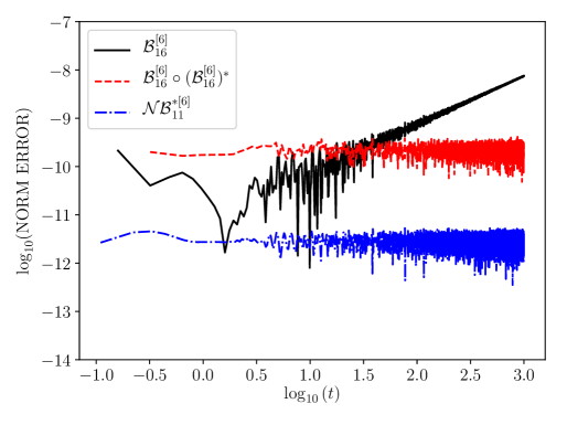
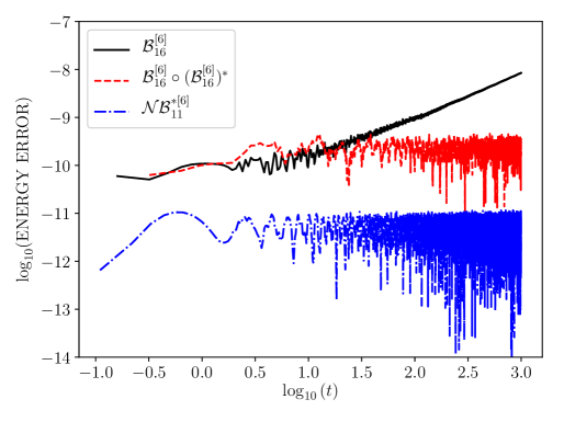
Figure 4: Error in norm $\mathcal{M}(u)$ (left) and in energy $\mathcal{H}(u)$ (right) as a function of time for complex-conjugate and palindromic methods involving complex coefficients.

In our second experiment, we test the efficiency of the different schemes. To this end we integrate until the final time $t_{f}=100$, compute the expectation value of the energy,$\mathcal{H}(u_{\mathrm{app}}(t))$, and measure the error as the maximum of the difference with respect to the exact value along the integration:

$$\max_{0\leq t\leq t_{f}}\quad|\mathcal{H}(u_{\mathrm{app}}(t))-\mathcal{H}(u_{0})|.$$ (5.2)

The corresponding results are displayed as a function of the computational cost measured by the number of FFTs necessary to carry out the calculations (in log-log plots) in Figure 5. Notice how the new symmetric-conjugate schemes offer a better efficiency than standard splitting methods for this problem. The improvement is particularly significant in the 6th-order case.

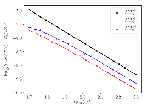
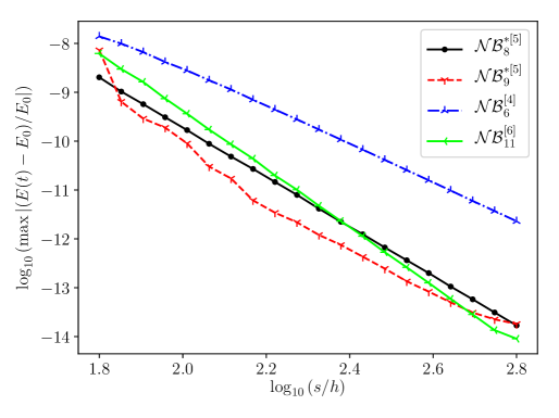
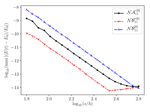
Figure 5: Maximum error in the expectation value of the energy along the integration for several 4th-, 5th- and 6th-order symmetric-conjugate splitting methods for the modified Pöschl–Teller potential.

Acknowledgements

The work of JB is supported by ANR-22-CE40-0016 “KEN” of the Agence Nationale de la Recherche (France) and by the region Pays de la Loire (France) through the project “MasCan”. SB, FC and AE-T acknowledge financial support by Ministerio de Ciencia e Innovación (Spain) through project PID2019-104927GB-C21, MCIN/AEI/10.13039/501100011033, ERDF (“A way of making Europe”). The authors would also like to thank Prof. C. Lubich for his very useful remarks.

Compliance with Ethical Standards

All authors declare that they have no conflicts of interest.

Appendix A Appendix

We collect in this Appendix the most efficient symmetric-conjugate splitting methods with $a_{j}>0$ and $b_{j}\in\mathbb{C}$ with $\Re(b_{j})>0$ we have found for a general problem of the form $H=A+B$. The coefficients of the schemes in boldface in Table 3 are listed in Table 4. Methods of type (4.4) of order $p$ involving $s$ stages are denoted as $\mathcal{A}_{s}^{*[p]}$, whereas $\mathcal{B}_{s}^{*[p]}$ refers to a similar scheme of type (4.5). As in Table 1, we also collect for reference the methods proposed in [10] (denoted by $\mathcal{GB}_{s}^{*[p]}$) and two efficient palindromic compositions of time-symmetric schemes of order 2 with real coefficients, $\mathcal{S}_{s}^{[p]}$. At order 5, the most efficient scheme turns out to be $\mathcal{GB}_{9}^{*[5]}$.

We also include a numerical illustration on the modified Pöschl–Teller potential with the same data as before. Notice in particular the improvement with respect to the 6th-order scheme $\mathcal{S}_{10}^{[6]}$.

	$\Delta_{a}$	$\Delta_{b}$	$E_{f}^{(4)}$	$E_{f}^{(5)}$	$E_{f}^{(6)}$	$E_{f}^{(7)}$	$E_{f}^{(8)}$	$E_{f}^{(9)}$
$\boldsymbol{\mathcal{B}_{3}^{*[3]}}$	1.000	1.766	0.522	0.509	0.682	0.664	0.812	0.875
$\mathcal{A}_{6}^{*[4]}$	1.000	1.125	–	0.410	0.827	0.608	1.090	0.988
$\boldsymbol{\mathcal{B}_{5}^{*[4]}}$	1.000	1.146	–	0.399	0.764	0.569	0.972	0.772
$\mathcal{B}_{6}^{*[4]}$	1.000	1.136	–	0.445	0.911	0.626	1.158	0.881
$\mathcal{A}_{9}^{*[5]}$	1.000	1.704	–	–	1.141	1.173	1.521	1.744
$\mathcal{B}_{9}^{*[5]}$	1.000	1.480	–	–	0.885	0.826	1.198	1.493
$\mathcal{A}_{15}^{*[6]}$	1.000	1.355	–	–	–	1.544	1.335	2.348
$\boldsymbol{\mathcal{B}_{15}^{*[6]}}$	1.000	1.327	–	–	–	1.150	1.274	2.116
$\mathcal{GB}_{3}^{*[3]}$	1.000	1.155	0.586	0.445	0.722	0.642	0.777	0.772
$\mathcal{GB}_{5}^{*[4]}$	1.000	1.133	–	0.480	0.698	0.676	0.918	0.830
$\boldsymbol{\mathcal{GB}_{9}^{*[5]}}$	1.000	1.463	–	–	0.681	0.819	1.126	1.439
$\mathcal{GB}_{15}^{*[6]}$	1.000	1.692	–	–	–	1.583	1.445	2.361
$\mathcal{S}_{6}^{[4]}(aba)$	1.168	1.575	–	0.559	–	0.792	–	1.239
$\mathcal{S}_{10}^{[6]}(aba)$	3.203	1.595	–	–	–	1.144	–	1.606

Table 3: 1-norm and effective errors for symmetric-conjugate splitting methods for $H=A+B$.

	$a_{i}$	$b_{i}$
$\mathcal{B}_{3}^{*[3]}$	$a_{0}=0.4706$	$b_{0}=0.1655101882118+0.03704896872215\,i$
	$a_{1}=1-2a_{0}$	$\Re(b_{1})=\frac{1}{2}-\Re(b_{0})-0.6300845020773\,i$
$\mathcal{B}_{5}^{*[4]}$	$a_{0}=\frac{37}{250}$	$b_{0}=0.05338438633498185-0.03218942894140047\,i$
	$a_{1}=0.22446218092466344$	$b_{1}=0.19561815336463223+0.0992879758243923\,i$
	$a_{2}=1-2\sum_{i=0}^{1}a_{i}$	$b_{2}=\frac{1}{2}-\sum_{i=0}^{1}\Re(b_{i})-0.14783578044680548\,i$
$\mathcal{B}_{15}^{*[6]}$	$a_{0}=0.08092666015955027$	$b_{0}=\frac{3}{100}-0.0028985018717006387\,i$
	$a_{1}=0.06736427978832901$	$b_{1}=0.08826477458499815+0.019065371639195743\,i$
	$a_{2}=0.057276240999706116$	$b_{2}=0.07026507350715319-0.05226928459003309\,i$
	$a_{3}=0.06428730473896961$	$b_{3}=0.051044248093469226+0.07580262639617709\,i$
	$a_{4}=0.05528732144478408$	$b_{4}=0.040506044227148555-0.07981221177569087\,i$
	$a_{5}=0.02566179136566552$	$b_{5}=0.03061653536468681+0.07254698089135206\,i$
	$a_{6}=0.10559039215618958$	$b_{6}=0.10349890449629792-0.03539199012223482\,i$
	$a_{7}=1-2\sum_{i=0}^{6}a_{i}$	$b_{7}=\frac{1}{2}-\sum_{i=0}^{6}\Re(b_{i})+0.0111821298374971054\,i$

Table 4: Coefficients of the most efficient splitting methods collected in Table 3.

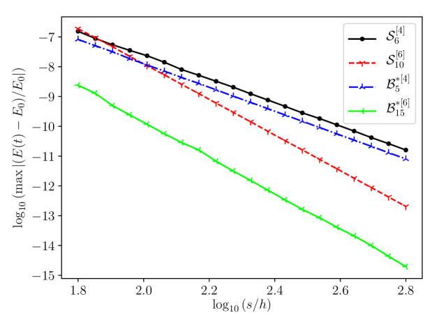
Figure 6: Maximum error in the expectation value of the energy along the integration as a function of the computational cost for the new symmetric-conjugate splitting methods intended for general problems of the form $H=A+B$ (modified Pöschl–Teller potential).

References

- [1] A. Bandrauk and H. Shen, Improved exponential split operator method for solving the time-dependent Schrödinger equation, Chem. Phys. Lett., 176 (1991), pp. 428–432.
- [2] S. Blanes and F. Casas, A Concise Introduction to Geometric Numerical Integration, CRC Press, 2016.
- [3] S. Blanes, F. Casas, P. Chartier, and A. Escorihuela-Tomàs, On symmetric-conjugate composition methods in the numerical integration of differential equations, Math. Comput., 91 (2022), pp. 1739–1761.
- [4] S. Blanes, F. Casas, and A. Escorihuela-Tomàs, Applying splitting methods with complex coefficients to the numerical integration of unitary problems, J. Comput. Dyn., 9 (2022), pp. 85–101.
- [5] S. Blanes, F. Casas, and A. Escorihuela-Tomàs, Runge–Kutta–Nyström symplectic splitting methods of order 8, Appl. Numer. Math., 182 (2022), pp. 14–27.
- [6] S. Blanes, F. Casas, and A. Murua, On the linear stability of splitting methods, Found. Comp. Math., 8 (2008), pp. 357–393.
- [7] S. Blanes, F. Casas, and A. Murua, Splitting and composition methods in the numerical integration of differential equations, Bol. Soc. Esp. Mat. Apl., 45 (2008), pp. 89–145.
- [8] F. Castella, P. Chartier, S. Descombes, and G. Vilmart, Splitting methods with complex times for parabolic equations, BIT Numer. Math., 49 (2009), pp. 487–508.
- [9] S. Flügge, Practical Quantum Mechanics, Springer, 1971.
- [10] F. Goth, Higher order auxiliary field quantum Monte Carlo methods, Tech. Rep. 2009.0449, arXiv, 2020.
- [11] F. Goth, Higher order auxiliary field quantum Monte Carlo methods, J. Phys.: Conf. Ser., 2207 (2022), p. 012029.
- [12] E. Hairer, C. Lubich, and G. Wanner, Geometric Numerical Integration. Structure-Preserving Algorithms for Ordinary Differential Equations, Springer-Verlag, Second ed., 2006.
- [13] E. Hansen and A. Ostermann, Exponential splitting for unbounded operators, Math. Comput., 78 (2009), pp. 1485–1496.
- [14] E. Hansen and A. Ostermann, High order splitting methods for analytic semigroups exist, BIT Numer. Math., 49 (2009), pp. 527–542.
- [15] T. Jahnke and C. Lubich, Error bounds for exponential operator splittings, BIT, 40 (2000), pp. 735–744.
- [16] C. Lubich, From Quantum to Classical Molecular Dynamics: Reduced Models and Numerical Analysis, European Mathematical Society, 2008.
- [17] R. McLachlan and R. Quispel, Splitting methods, Acta Numerica, 11 (2002), pp. 341–434.
- [18] M. Thalhammer, Convergence analysis of high-order time-splitting pseudo-spectral methods for nonlinear Schrödinger equations, SIAM J. Numer. Anal., 50 (2012), pp. 3231–3258.