[2303.10937] Boosting Weakly Supervised Object Detection using Fusion and Priors from Hallucinated Depth (Supplementary File)

Appendix S.1 Alternative approach for depth priors

	Avg. Precision, IoU			Avg. Precision, Area
Methods on COCO	0.5:0.95	0.5	0.75	S	M	L
MIST [ren2020instance] w/ EM	8.5	17.9	7.3	3.0	9.4	14.9
+ Siamese-Only	8.8	18.7	7.3	2.9	9.6	15.4
+ Depth-Oicr-Alt	8.9	19.0	7.3	3.0	9.6	15.6
+ Depth-Oicr	9.0	19.4	7.3	3.1	9.6	15.9
+ Depth-Attention-Alt	9.0	18.8	7.7	3.0	9.5	16.0
+ Depth-Attention	9.1	19.0	7.9	3.0	9.5	16.2

Table S.1: This table introduces the comparison of the proposed and alternate approaches (Depth-Oicr-Alt and Depth-Attention-Alt) for modeling depth priors. All proposed methods that outperform the Siamese-Only are underlined.

In Sec. 3.3, we described our method to obtain depth priors leveraging generated bounding box predictions and associated captions to extract knowledge about the relative depths of objects. As an alternative, we use only bounding box predictions (without captions) to obtain depth priors.

Similar to Sec. 3.3, let $C$ be the set of object categories, and $B$ be the set of predicted bounding boxes. Let $d_{c,b}\in[0,1]$ denote the depth value for object $c\in C$ and box $b\in B$ . Further, $d_{c}$ represents a set of depth values for each $c$ . The depth range $r_{c}=[mean-std,mean+std]$ is obtained by utilizing the mean and standard deviation (std) of this set of depth values in $d_{c}$ .

Table S.1 demonstrates that the Depth-Oicr-Alt and Depth-Attention-Alt techniques, employed from the alternate approach, yield superior results compared to Siamese-Only. Nevertheless, the Depth-Oicr and Depth-Attention methods, derived from the proposed approach, outperform both Depth-Oicr-Alt and Depth-Attention-Alt. Note that the depth range $r_{c}$ remains consistent across all images in this alternative method. Conversely, in the proposed approach, the depth range $dr_{c}$ is computed individually for each image by taking into account the corresponding caption, as visualized in Figure 3 of the paper. As a result, the proposed approach demonstrates enhanced capacity in modeling depth priors through the utilization of captions.

Appendix S.2 Depth modality in inference

As detailed in Section 3.2, fusion scores ( $f^{det}$ and $f^{cls}$ ) are calculated by adding together RGB scores ( $v^{det}$ and $v^{cls}$ ) and depth scores ( $d^{det}$ and $d^{cls}$ ) in Eq. 5. Then, fusion scores are used to compute multiple instance learning loss $\mathcal{L}_{mil}$ in Eq. 9 to derive region-level scores during training. However, our proposed method uses only RGB detection $v^{det}$ and classification $v^{cls}$ scores during inference.

	Avg. Precision, IoU			Avg. Precision, Area
Methods on COCO	0.5:0.95	0.5	0.75	S	M	L
MIST [ren2020instance]	11.8	24.3	10.7	3.6	13.2	18.9
+ Wsod-Amplifier (Ours)	13.8	27.8	12.5	4.6	14.8	22.6
+ Wsod-Amplifier-Depth	4.4	8.7	3.8	0.6	3.5	8.8
+ Wsod-Amplifier-Fusion	13.1	27.5	11.9	4.3	14.3	22.2

Table S.2: This table compares the different variations of our Wsod-Amplifier method during inference. The best performer per column is in bold.

The performance of Wsod-Amplifier-Depth, which relies solely on depth scores during inference, is poorer due to the relatively lower informativeness of depth images compared to RGB images for detection in Table S.2. On the other hand, Wsod-Amplifier-Fusion, which employs fusion scores, exhibits lower performance than our proposed approach, Wsod-Amplifier, which solely employs RGB scores during inference. The rationale behind the enhancement of results through fusion during training, while not during inference, stems from the nature of the MIL loss $\mathcal{L}_{mil}$ . This loss function is formulated to guide the model in the classification of objects in an image, indirectly yielding region-level detection scores. While training, inaccuracies in depth for certain regions can be compensated by other regions to classify objects in MIL loss. However, during inference, each region operates independently, and errors on a per-region basis more directly impact detection results. Further, [meyer2020improving] demonstrates that integrating the depth modality with RGB aids in enhancing the model’s performance in classification tasks. The improved classification capacity of our model consequently leads to enhanced benefits from the MIL loss, contributing to improved representation learning. This improvement is highlighted by the enhanced performance of RGB scores during inference.

Objects	# of Instances	STD	MIST [ren2020instance] w/ EM	+ Wsod-Amplifier
Bear	902	15	19.9	36.6 (+16.7)
Toilet	2860	17	4.7	20.3 (+15.6)
Train	3157	15	14.3	26.3 (+12.0)
TV	4031	18	11.3	19.2 (+7.9)
Giraffe	3593	14	8.0	13.6 (+5.6)
Zebra	3653	16	22.4	27.9 (+5.5)
Airplane	3823	15	28.7	33.9 (+5.2)
Elephant	3876	14	26.4	31.1 (+4.7)
Refrigerator	1872	16	8.8	13.5 (+4.7)
Cat	3298	17	7.8	11.8 (+4.0)
Pizza	3993	17	32.2	35.9 (+3.7)
Horse	4645	15	21.5	25.1 (+3.6)
Fire hydrant	1313	15	24.8	28.4 (+3.6)
Sheep	6442	16	11.3	14.5 (+3.2)
Cow	5588	16	19.7	22.8 (+3.1)
Dog	3764	16	8.7	11.7 (+3)
Truck	7043	17	9.7	12.6 (+2.9)
Cake	4508	15	6.2	9.0 (+2.8)
Parking meter	833	14	23.7	26.4 (+2.7)
Sandwich	3069	15	8.0	10.6 (+2.6)
Bird	7100	19	8.8	11.3 (+2.5)
Kite	6333	17	11.2	13.6 (+2.4)
Carrot	5463	18	1.7	4.0 (+2.3)
Broccoli	4894	18	5.3	7.6 (+2.3)
Clock	4310	18	13.0	15.3 (+2.3)
Motorcycle	5971	15	15.4	17.5 (+2.1)
Tennis racket	3397	16	1.7	3.7 (+2.0)
Keyboard	1978	18	1.4	3.3 (+1.9)
Donut	4854	17	12.3	14.0 (+1.7)
Cell phone	4449	17	11.5	13.1 (+1.6)
Apple	4244	17	5.0	6.5 (+1.5)
Car	30530	18	6.1	7.6 (+1.5)
Banana	6698	17	5.6	7.1 (+1.5)
Chair	26825	16	1.5	2.8 (+1.3)
Hot dog	1997	14	7.8	9.0 (+1.2)
Umbrella	7729	17	6.9	8.1 (+1.2)
Wine glass	5559	18	0.4	1.5 (+1.1)
Sink	3929	17	0.1	1.2 (+1.1)
Bench	6739	18	6.1	7.0 (+0.9)
Microwave	1188	18	0.8	1.6 (+0.8)
Bed	2903	12	27.6	28.4 (+0.8)
Vase	4593	17	0.7	1.4 (+0.7)
Bowl	10020	19	11.7	12.4 (+0.7)
Bus	4317	16	35.5	36.2 (+0.7)
Laptop	3406	17	30.2	30.8 (+0.6)
Bottle	16782	21	4.6	5.2 (+0.6)
Boat	7449	17	4.2	4.7 (+0.5)
Bicycle	4912	18	9.8	10.3 (+0.5)
Teddy bear	3397	17	17.6	17.9 (+0.3)
Cup	14454	20	3.8	4.0 (+0.2)
Snowboard	1956	16	0.0	0.2 (+0.2)
Surfboard	4133	15	0.2	0.4 (+0.2)
Stop sign	1372	16	48.0	48.2 (+0.2)
Couch	4111	16	1.2	1.3 (+0.1)
Book	16826	21	0.1	0.2 (+0.1)
Scissors	1059	19	0.1	0.1
Skis	4683	14	0.1	0.0 (-0.1)
Suitcase	4188	15	3.8	3.6 (-0.2)
Person	181524	19	1.4	1.0 (-0.4)
Traffic light	9115	17	5.9	4.7 (-1.2)
Frisbee	1861	17	6.8	4.8 (-2.0)
Orange	4525	18	13.1	10.6 (-2.5)
Oven	2302	19	9.7	5.7 (-4.0)
Total	597245	15	8.5	10.2 (+1.7)

Table S.3: The table provides class-wise

mAP_{50:95}

results for both MIST [ren2020instance] with EM and our Wsod-Amplifier. The objects are sorted according to the change in performance. Additionally, the table provides information about the standard deviation (STD) and the number of instances within the training set. Note that 17 object categories from the COCO dataset have been excluded from this table due to both methods yielding a

mAP

of zero.

Appendix S.3 Class-wise comparison on COCO

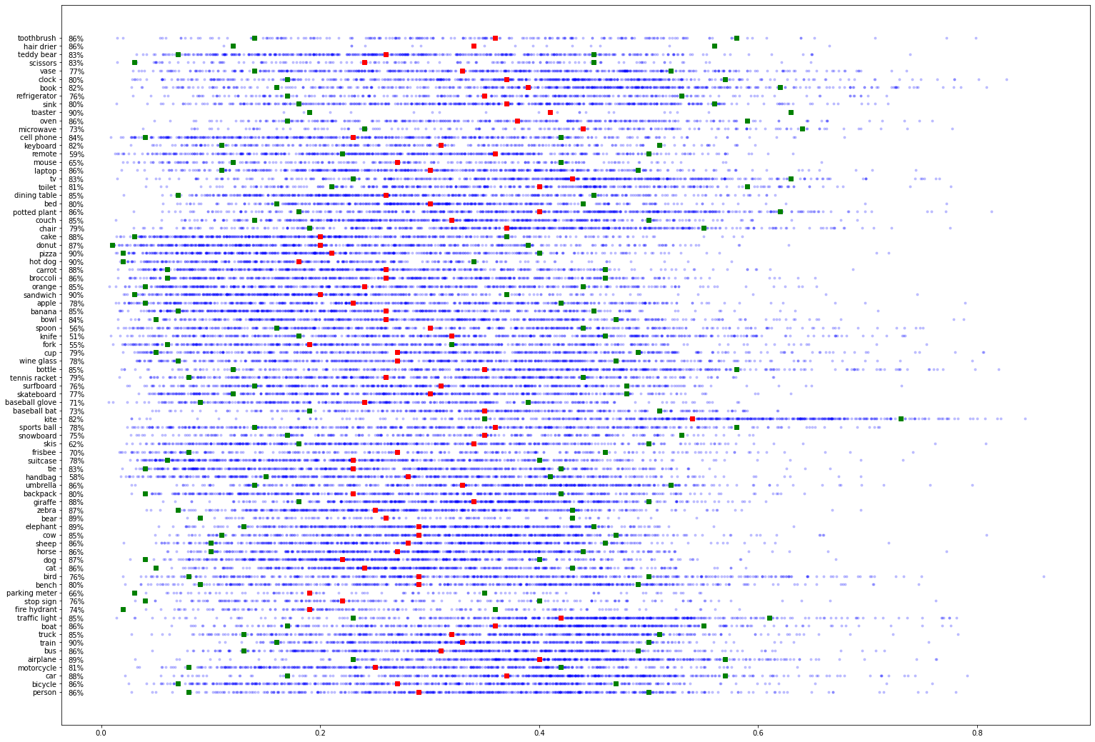
Figure S.2 demonstrates the effectiveness of depth priors in capturing the depth characteristics of different object classes in the COCO dataset. On average across classes, a substantial portion of the training data (80.75%), resides within the constant ranges $r_{c}$ in the figure. Note the depth ranges $dr_{c}$ in our proposed approach for depth priors are computed separately for each image according to the corresponding caption. This image-specific calculation achieves more comprehensive coverage of depth variations within the training data compared to constant ranges $r_{c}$ . Diverse object classes exhibit distinct depth ranges. The ”fire hydrant” object displays the smallest average depth mean at 19%, whereas the ”kite” object displays the highest (54%).

Appendix S.4 Scalability and generalization

Our demonstration reveals that a substantial amount of data is not necessary for estimating depth. The depth priors calculated from the least frequent classes contribute even more to performance improvement than those from the most frequent classes. Referring to the data presented in Table S.3, the average increase in $mAP_{50:95}$ for the least frequent 20% classes is 3.4, while the increase for the most frequent 20% classes is 0.8.

To understand the impact of diverse depth ranges on performance, Table S.3 includes per-class standard deviations (STD). Notably, the depth priors computed from classes with smaller STDs make a more significant contribution to performance enhancement compared to those with larger STDs. On average, the $mAP_{50:95}$ increase for the 20% of classes with the smallest STD is 4.8, whereas the increase for the 20% of classes with larger STDs is 1.2. The observation suggests that a narrower depth distribution of an object corresponds to more informative depth information. Certainly, objects like ”bear,” ”train,” and ”giraffe” exhibit smaller STDs, thereby leading to a more significant improvement in detection performance. Additionally, respective percentages of objects in Figure S.2, which depict the proportion of training data within the specified depth range, are notably higher at 89%, 90%, and 88%, respectively.

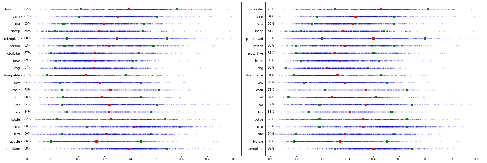
Our analysis demonstrates that depth priors calculated using COCO exhibit similarities to those computed using PASCAL, as evident from Figure S.3. On an average basis across various classes, approximately 84.4% of data aligns within the constant ranges derived from PASCAL, whereas 82.3% aligns within the ranges from COCO. The minimal differences in percentage and the visual resemblance of depth ranges in Figure S.3 underscore the generalizability of our depth priors. Furthermore, we mention in Sec. 4.3 that applying the depth priors calculated from COCO to Conceptual Captions (CC) results in a more significant performance improvement on the noisy CC compared to COCO, even though priors are computed from COCO.

Methods	Clipart	Watercolor	Comic
MIST [ren2020instance] w/ GT	9.4	13.3	9.2
+ Wsod-Amplifier	10.2	14.7	9.6

Table S.4: This table introduces the improvement of our Wsod-Amplifier over MIST on domain shift datasets. The results are in

mAP_{50}

metric. The best performer per column is in bold.

Refer to caption — Figure S.1: This figure provides an intuitive understanding of how the utilization of captions enhances the estimation of the depth range $dr_{c}$ of class c for a specific image. Here, $r_{c,w}$ signifies the depth range of class c when it is associated with the word w.

Appendix S.5 Generalization to appearance changes

By relying on depth information, our method builds some robustness to overfitting to appearance, which may not be the same across datasets. To test this hypothesis, we conduct experiments with domain shift datasets [inoue2018cross]. Table S.4 shows that our Wsod-Amplifier boosts the performance of MIST baseline in $mAP_{50}$ by $4-10\%$ , even though no training is performed on these datasets.

Appendix S.6 Illustration to depth ranges with caption

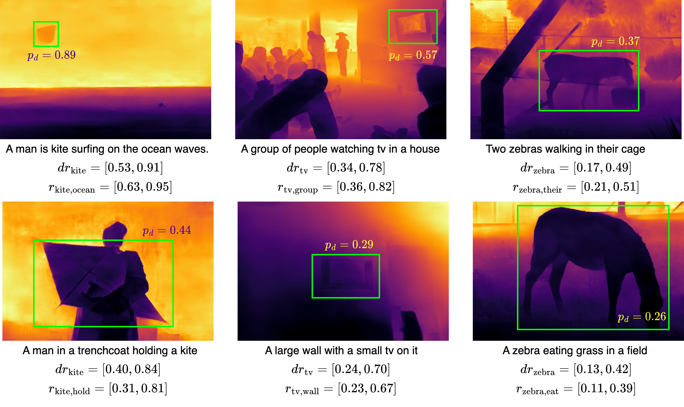
The depth range $dr_{c}$ for class $c$ is individually computed for each image by leveraging the corresponding caption. In this context, $r_{c,w}$ denotes the depth range of class $c$ when linked to the word $w$ . In Eq. 10, the calculation of $dr_{c}$ involves deriving the average of depth ranges $r_{c,w}$ across each word present within the caption. Figure S.1 illustrates three object examples: ”kite”, ”TV”, and ”zebra”. The top row of images depicts instances where objects are situated farther away from the camera, while the bottom row showcases examples where objects are positioned closer to the camera. As an illustration, consider the ”kite” object in the upper image, where the caption features the word ”ocean.” Due to the influence of $r_{kite,ocean}$ , the depth range $dr_{kite}$ becomes larger. It’s reasonable to expect that a kite would be positioned at a greater distance from the camera if it’s flying over an ocean. Worth noting is that while $dr_{kite}$ is enlarged, it remains smaller than $r_{kite,ocean}$ due to the averaging effect with less descriptive words like “is.” In a similar scenario, the depth range $dr_{kite}$ in the lower image becomes smaller due to the impact of $r_{kite,holding}$ . When a person holds a kite, the likelihood is that the kite is positioned closer to the camera.

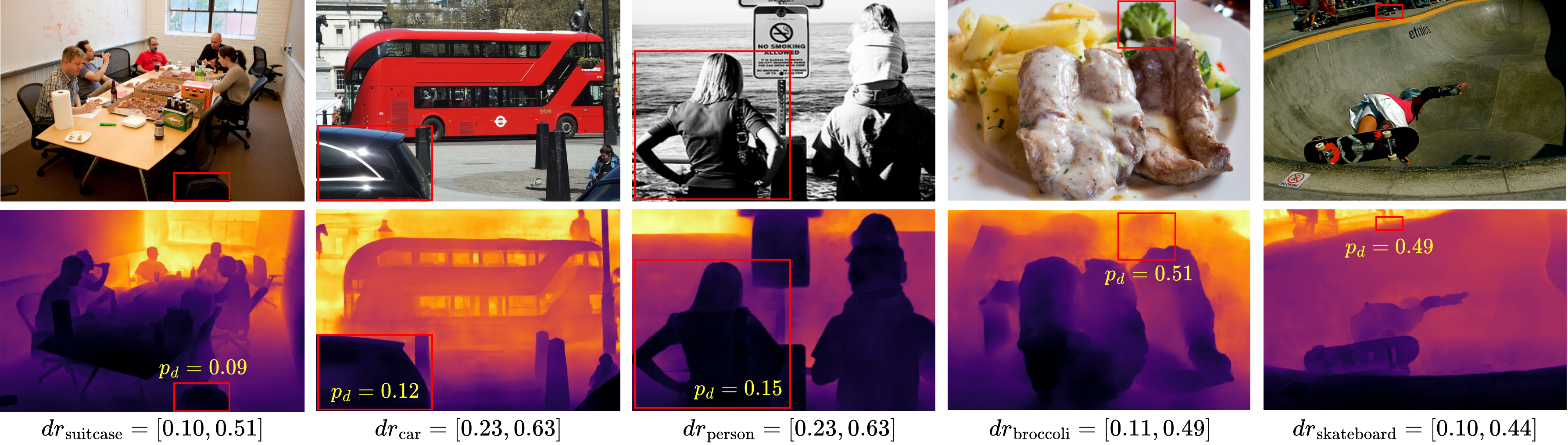
Appendix S.7 Failure cases

In Figure S.4, the initial three cases depict objects with smaller depth values lying outside the depth range, while the last two cases feature objects with larger depth values. In the second scenario, the car is positioned closer to the camera, causing it to exceed the depth range limits. In contrast, in the fourth scenario, the broccoli is situated in the background with a larger depth value.