Strong lensing and shadow of Ayon-Beato-Garcia (ABG) nonsingular black hole

Abstract

We study nonsingular black holes viewed from the point of view of Ayon-Beato-Garcia (ABG) nonlinear electrodynamics (NLED) and present a complete study of their corresponding strong gravitational lensing. The NLED modifies the the photon’s geodesic, and our calculations show that such effect increases the corresponding photon sphere radius and image separation, but decreases the magnification. We also show that the ABG’s shadow radius is not compatible with bound estimates of Sgr A* from Keck and VLTI (Very Large Telescope Interferometer). Thus, the possibility of Sgr A* being a nonsingular ABG black hole is ruled out.

I Introduction

Black hole (BH) is one of the most straightforward yet profound prediction of General Relativity (GR). Its extreme gravity distorts its surrounding spacetime and bends light, creating (among many things) the gravitational lensing phenomenon. The recent observation by Event Horizon Telescope (EHT) that successfully captured the visual images of the superheavy BHs M87* EventHorizonTelescope:2019dse and Sgr A* EventHorizonTelescope:2022wkp has established a triumph for the gravitational lensing as a means to empirically prove black hole’s existence. By “image” here is the corresponding shadow Falcke:1999pj surrounded by accreting materials that emits and lenses light from the nearby background source.

Theoretically, the study of gravitational lensing is as old as GR itself (see, for example, schneider:1992 ; Perlick:2004tq and the references therein), but it was Darwin who first applied it for Schwarzschild BH Darwin_gravity_1959 . His exact calculation on the deflection angle shows that at small impact parameters there exists a critical value (close to the corresponding photon sphere) where the deflection angle suffers from logarithmic divergence Bozza:2010xqn , beyond which photons fall into the horizon. His results were later rediscovered and developed by other authors, for example in Luminet:1979nyg ; AbhishekChowdhuri:2023ekr ; Ghosh:2022mka ; Chandrasekhar:1985kt . In the last two decades the study of gravitational lensing in the strong deflection limit received revival and extensive elaboration Frittelli:1999yf ; Bozza:2001xd ; Bozza:2002zj ; Virbhadra:1999nm . In particular, Bozza shows in Bozza:2002zj that the analytical expansion of the strong deflection angle in the limit of $r\rightarrow r_{ps}$ ($r_{ps}$ being the photon sphere radius) is given by

$$\alpha(b)=-\tilde{a}_{1}\log\left(\frac{b}{b_{c}}-1\right)+\tilde{a}_{2}+O(b-b_{c}).$$ (1)

with $\tilde{a}_{1}$ and $\tilde{a}_{2}$ some constants. Upon closer inspection, Tsukamoto gave correction to the higher order expansion Tsukamoto:2016qro ; Tsukamoto:2016jzh . The result on Schwarszchild was extended to the case of Reissner-Nordstrom by Eiroa et al Eiroa:2002mk , while the strong lensing in Kerr BH was studied in Bozza:2002af ; Vazquez:2003zm ; Bozza:2006nm .

Probably the most intriguing property of black holes is the existence of singularity due to the gravitational collapse Oppenheimer:1939ue . It was believed that such singularity is an inherent solution of general relativity, but the stable ones (like all observable black holes) are disconnected from the observers by event horizon Penrose:1964wq . Nevertheless, Bardeen in 1968 constructed a metric function that produced nonsingular spacetime bardeenNonsingularGeneralrelativisticGravitational1968 . The metric and all invariants are devoid of singularity everywhere, including at $r=0$. Instead, we have regular de Sitter space at the core. (For an excellent review on regular BH see, for example, Ansoldi:2008jw .) The strong lensing phenomenon around Bardeen BH has been studied in Eiroa:2010wm ; Wei:2015qca .

At first nobody knows what kind of matter that sources the Bardeen geometry, but later Ayon-Beato and Garcia (ABG) realized that this nonsingular metric can be obtained as solutions of Einstein’s equations coupled to some nonlinear electrodynamics (NLED) source Ayon-Beato:1998hmi ; Ayon-Beato:2000mjt . Invoking NLED turns out to have profound impact on the geodesic of test photon. Novello et al showed that in nonlinear electrodynamics background, photon moves in an effective modified geometry Novello:1999pg , and this radically modifies the corresponding optical observables. In Allahyari:2019jqz the authors model the M87* as (singular) NLED-charged black hole and studied its shadow.

In this work, we discuss the effect of effective geometry to the lensing phenomenon in the Bardeen BH using one of the ABG’s NLED model. In particular, we calculate the image separation and magnification. We use it as a model for the supermassive black hole at the center of our galaxy, the Sgr A*, and calculate the astrophysical observables. Lastly, we investigate its shadow radius and compare it to the astrophysical data from Keck and VLTI. This paper is organized as follows. In Sec. II we briefly review the regular Bardeen solution and its corresponding ABG models. In Sec. III we present the effective metric of ABG and the corresponding photon sphere. Sec. IV is devoted to applying the Bozza’s and Tsukamoto’s strong lensing formalism to our model. Sec. V is devoted to calculating the strong lensing observables using the Sgr A* data. In Sec. VI we calculate the shadow radius and plot it against the Keck-VLTI constraints. Finally, we summarize our findings in Sec. VII.

II Bardeen Spacetime

The Bardeen metric is given by bardeenNonsingularGeneralrelativisticGravitational1968 :

$$ds^{2}=-f(r)dt^{2}+f(r)^{-1}dr^{2}+r^{2}d\Omega^{2},$$ (2)

with

$$f(r)\equiv 1-\frac{2mr^{2}}{(r^{2}+q^{2})^{\frac{3}{2}}},$$ (3)

and $q$ is the charge. This spacetime is regular at $r=0$, as can easily be seen from the Kretschmann scalar:

$$\lim_{r\rightarrow 0}R^{\alpha\beta\gamma\delta}R_{\alpha\beta\gamma\delta}=\frac{96m^{2}}{q^{8/3}},$$ (4)

while the metric behaves de Sitter-like

$$f(r)\approx 1-\frac{2m}{q^{3}}r^{2}.$$ (5)

The horizons $r_{h}$ are given by the roots of

$$\left(r_{h}^{2}+q^{2}\right)^{3}-4m^{2}r_{h}^{4}=0.$$ (6)

Bardeen black hole can, in general, possess up to two horizons. The extremal condition is achieved when Ayon-Beato:2000mjt

$$q^{2}=\frac{16}{27}m^{2}\ \rightarrow r_{extr}=\sqrt{\frac{32}{27}}m.$$ (7)

Ayon-Beato and Garcia proposed the NLED matter to source the Bardeen spacetime, given in Ayon-Beato:1998hmi . This model, however, produces a slightly different metric function than the original Bardeen,

$$f(r)=1-\frac{2mr^{2}}{(r^{2}+q^{2})^{\frac{3}{2}}}+\frac{q^{2}r^{2}}{\left(r+2+q^{2}\right)^{2}}.$$ (8)

Strong lensing of this particular model has been discussed in Ghaffarnejad:2016dlw . Later ABG considered a simpler NLED sourced by magnetic monopole as follows Ayon-Beato:2000mjt ,

$$\mathcal{L}=\frac{3}{2sq^{2}}\left(\frac{\sqrt{2q^{2}F}}{1+\sqrt{2q^{2}F}}\right)^{5/2},$$ (9)

where $F\equiv\frac{1}{4}F^{\mu\nu}F_{\mu\nu}$ and $s\equiv q/2m$. By inserting the monopole ansatz $A_{\mu}=\delta^{\varphi}_{\mu}q\left(1-\cos\theta\right)$, the field strength becomes $F=q^{2}/2r^{4}$ and the Lagrangian produces the metric solution Eq. (3).

III Effective Geometry

The NLED Lagrangian above induces the effective metric tensor Novello:1999pg

$$g^{\mu\nu}_{eff}=g^{\mu\nu}-\frac{4\mathcal{L}_{FF}}{\mathcal{L}_{F}}F^{\mu}_{\alpha}F^{\alpha\nu},$$ (10)

where $\mathcal{L}_{A}\equiv\partial\mathcal{L}/\partial A$. This, in turn, yields the effective length element

$$ds^{2}_{eff}=-f(r)dt^{2}+f(r)^{-1}dr^{2}+h_{m}(r)r^{2}d^{2}\Omega,$$ (11)

where

$$h_{m}(r)=\left(1+\frac{4\mathcal{L}_{FF}}{\mathcal{L}_{F}}\frac{q^{2}}{r^{4}}\right)^{-1}.$$ (12)

Inserting the Lagrangian (9) we obtain

$$h_{ABG}(r)=\left(1-\frac{2(6q^{2}-r^{2})}{(q^{2}+r^{2})}\right)^{-1}.$$ (13)

From the corresponding geodesic equation it is not difficult to see that the radial equation satisfies

$$\frac{1}{2}\dot{r}^{2}+V_{eff}=0,$$ (14)

where we define the effective potential $V_{eff}$ as

$$V_{eff}\equiv\frac{f(r)}{h(r)}\frac{\mathbb{L}^{2}}{r^{2}}.$$ (15)

The corresponding photon sphere radius is given by the largest positive root of the following condition, Bozza:2002zj

$$\frac{f^{\prime}(r_{ps})}{f(r_{ps})}-\frac{2}{r_{ps}}-\frac{h^{\prime}(r_{ps})}{h(r_{ps})}=0.$$ (16)

This yields,

$$\frac{2}{r_{ps}}+\frac{28q^{2}r_{ps}}{11q^{4}+8q^{2}r_{ps}^{2}-3r_{ps}^{4}}+\frac{m\left(4q^{2}r_{ps}-2r_{ps}^{3}\right)}{\left(q^{2}+r_{ps}^{2}\right)\left[\left(q^{2}+r_{ps}^{2}\right)^{3/2}-2mr_{ps}^{2}\right]}=0.$$ (17)

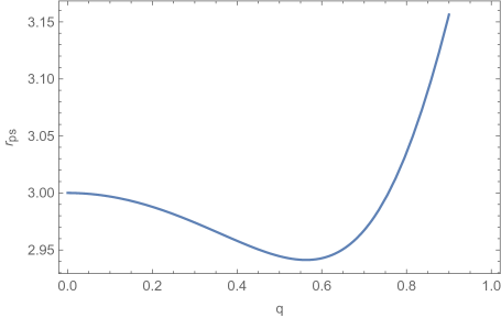
Figure 1: Photon Sphere of Bardeen with ABG source as function of charge ($q$) for $m=1$.

By solving the roots numerically, the behavior of $r_{ps}$ as a function of q, $r_{ps}=r_{ps}(m=1,q)$, is shown in Fig.1. It is shown that the photon sphere decreases as the charge increases until some critical value $q_{crit}$ where $r_{ps}(m=1,q=q_{crit})$ is minimum, beyond which $r_{ps}$ starts increasing without bound. Interestingly, the critical value $q_{crit}$ is not given by the extremal charge $q=\sqrt{16/27}m$, as in the Bardeen case. Rather, $q_{crit}=16/27\ m=0.592$.

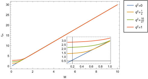
Figure 2: $r_{ps}$ as function of $m$ for a variation of charge $q$.

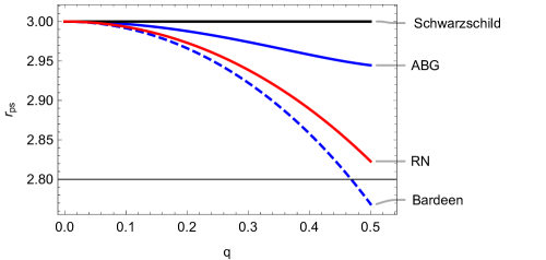
Figure 3: $r_{ps}$ as function of $q$ for different models.

In Fig. 2 we show how $r_{ps}$ varies with $m$ for several values of $q$. They differ only at small $m$. When the mass is large, $r_{ps}$ for different $q$ asymptote to a single gradient. In Fig. 3 we show the deviation of $r_{ps}$ as a function of $q$ from the Schwarzschild (charge-less condition). The ABG model we consider here falls between the Schwarzschild and the RN at large $q$, unlike the original Bardeen which falls the fastest.

IV Deflection Angle in the Strong Field Limit

From the spherical symmetry and staticity conditions, Noether’s theorem dictates that this spacetime has constants of motion, the total test particle’s energy $E$ and angular momentum $\mathbb{L}$, related to the $\partial_{t}$ and $\partial_{\varphi}$ Killing vectors, respectively. We define the impact parameter for photon as

$$b(r_{0})\equiv\frac{\mathbb{L}}{E}=\sqrt{\frac{h_{m}(r_{0})r_{0}^{2}}{f(r_{0})}}.$$ (18)

Solving the null geodesic equation, the general expression for bending angle of light rays can be expressed as (see, for example, in Weinberg:1972kfs )

$$\alpha(r_{0})=2\int_{r_{0}}^{\infty}\sqrt{\frac{1}{r^{2}f(r)h(r)R(r)}}dr-\pi,$$ (19)

where

$$R(r)=\frac{r^{2}h(r)}{b^{2}f(r)}-1.$$ (20)

The integral is divergent at $r_{0}\rightarrow r_{ps}$. To circumvent this problem we define $z\equiv 1-r_{0}/r$ Tsukamoto:2016jzh and write Eq. (19) as

$$\alpha(r_{0})=\int^{1}_{0}\mathcal{H}(z,r_{0})dz-\pi,$$ (21)

with

$$\mathcal{H}(z,r_{0})\equiv\frac{2\left(1-z\right)^{2}}{\sqrt{f\left(\frac{r_{0}}{1-z}\right)h\left(\frac{r_{0}}{1-z}\right)R\left(\frac{r_{0}}{1-z}\right)}}.$$ (22)

The singular part can be isolated by defining

$$\mathcal{H}(z,r_{0})\equiv\mathcal{H}_{R}(z,r_{0})+\mathcal{H}_{D}(z,r_{0}),$$ (23)

where the subscript R(D) refers to the regular (divergent) part, respectively.

To handle the divergent part:

$$\mathcal{I}_{D}(r_{0})\equiv\int^{1}_{0}\mathcal{H}_{D}(z,r_{0})dz,$$ (24)

we define $\mathcal{H}(z,r_{0})\equiv 2r_{0}/\sqrt{\mathcal{G}(z,r_{)}}$ and, by expanding it around $z\rightarrow 0$, obtain the expression for $\mathcal{G}(z,r_{0})$ up to second-order:

$$\mathcal{G}_{0}(z,r_{0})=c_{1}(r_{0})z+c_{2}(r_{0})z^{2},$$ (25)

where

$$c_{1}(r_{0}) = C_{0}\mathcal{D}_{0}r_{0}f(r_{0}),$$

$$c_{2}(r_{0}) = C_{0}r_{0}f_{0}\bigg{\{}\mathcal{D}_{0}\left[\mathcal{D}_{0}\left(\mathcal{D}_{0}+\frac{f^{\prime}_{0}}{f_{0}^{3}}\right)r_{0}-3\right]+\frac{\mathcal{D}_{0}r_{0}}{2}\bigg{\}},$$ (26)

with $X_{0}\equiv X(r=r_{0})$, $C(r)\equiv h(r)r^{2}$, and

$$\mathcal{D}(r)\equiv\frac{C^{\prime\prime}(r)}{C(r)}-\frac{f^{\prime\prime}(r)}{f(r)}.$$ (27)

For the ABG model, the values of $c_{1}$ and $c_{2}$ are

$$c_{1}(r_{0}) = -\frac{2(r_{0}^{2}(11q^{4}+22q^{2}r_{0}^{2}-3r_{0}^{4})\tilde{j}_{1}^{3/2}+m(9r_{0}^{8}-61q^{2}r_{0}^{6})))}{(11q^{2}-3r^{2})^{2}\tilde{j}_{1}^{3/2}},$$

$$c_{2}(r_{0}) = \frac{mr_{0}^{6}\tilde{j}_{2}+r_{0}^{2}(\tilde{j}_{3}\tilde{j}_{1}^{5/2}-\tilde{j}_{3})}{(11q^{2}-3r_{0}^{2})^{3}\tilde{j}_{1}^{5/2}},$$

with

$$\tilde{j}_{1} \equiv q^{2}+r_{0}^{2},$$

$$\tilde{j}_{2} \equiv 2013q^{6}+3104q^{4}r_{0}^{2}+57q^{2}r_{0}^{4}-54r_{0}^{6},$$

$$\tilde{j}_{3} \equiv 121q^{6}+825q^{4}r_{0}^{2}-99Q^{2}r_{0}^{4}+9r_{0}^{6}.$$ (29)

Following Bozza Bozza:2002zj and Tsukamoto Tsukamoto:2016jzh it can be shown that the divergent integral in the strong field limit $r\rightarrow r_{ps}$ (or equivalently $b\rightarrow b_{ps}$) is expressed as

$$\mathcal{I}_{D}(b) = -\sqrt{\frac{2}{f_{ps}C_{ps}^{\prime\prime}-f^{\prime\prime}_{ps}C_{ps}}}$$

$$\times\bigg{\{}\log\left(\frac{b}{b_{c}}-1\right)+\log\left[r_{ps}^{2}\left(\frac{C_{ps}^{\prime\prime}}{C_{ps}}-\frac{f_{ps}^{\prime\prime}}{f_{ps}}\right)\right]\bigg{\}}.$$

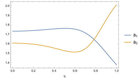
Figure 4: The values of $\tilde{a}_{1}$ and $\tilde{a}_{2}$ for Bardeen with ABG source

The regular part is

$$\mathcal{I}_{R}\equiv\int^{1}_{0}\mathcal{H}_{R}(z,r_{0})dz.$$ (31)

Likewise, by expanding around $r\rightarrow r_{ps}$ the integral can be expressed as

$$\frac{\mathcal{I}_{R}(r_{ps})}{2r_{ps}} = \int^{1}_{0}\frac{dz}{F(r_{ps},z)}-\int^{1}_{0}\sqrt{\frac{2}{C_{ps}r_{ps}f_{ps}\mathcal{D}_{ps}z^{2}}}dz,$$

with

$$F(r_{ps},z)\equiv\sqrt{C\left(\frac{r_{ps}}{1-z}\right)R\left(\frac{r_{ps}}{1-z}\right)f\left(\frac{r_{ps}}{1-z}\right)\left(1-z\right)^{4}}.$$ (33)

For the ABG model, the integral can be evaluated numerically. Putting (IV) and (IV) into (21), we can express it as Eq. (1) by identifying

$$\tilde{a}_{1} \equiv \sqrt{\frac{2A_{ps}B_{ps}}{A_{ps}C^{\prime\prime}_{ps}-A^{\prime\prime}_{ps}C_{ps}}},$$

$$\tilde{a}_{2} \equiv \tilde{a_{1}}\log\tilde{b}+I_{R}(r_{ps})-\pi,$$ (34)

with

$$\tilde{b}\equiv r_{ps}^{2}\left(\frac{C^{\prime\prime}_{ps}}{C_{ps}}-\frac{A^{\prime\prime}_{ps}}{A_{ps}}\right).$$ (35)

In terms of the ABG model we consider, their expressions are

$$\tilde{a}_{1} = \sqrt{\frac{(11q^{2}-3r_{ps}^{2})^{3}\tilde{k}_{1}^{5/2}}{\tilde{k}_{2}-\tilde{k}_{3}\tilde{k}_{1}^{5/2}}},$$

$$\tilde{a}_{2} = -\pi+\mathcal{I}_{R}(r_{ps})+\sqrt{\frac{(11q^{2}-3r_{ps}^{2})^{3}\tilde{k}_{1}^{5/2}}{\tilde{k}_{2}-\tilde{k}_{3}\tilde{k}_{1}^{5/2}}}\log\left[\frac{2\tilde{k}_{1}^{5/2}\tilde{k}_{3}-2\tilde{k}_{2}}{(11q^{2}-3r_{ps}^{2})^{2}(\tilde{k}_{1}^{3/2}-2mr_{ps}^{2})\tilde{k}_{1}^{2}}\right],$$

with

$$\tilde{k}_{1} = q^{2}+r_{ps}^{2},$$

$$\tilde{k}_{2} = m(3355q^{6}r_{ps}^{4}+466q^{4}r_{ps}^{6}+51q^{2}r_{ps}^{8}),$$

$$\tilde{k}_{3} = (121q^{6}+825q^{4}r_{ps}^{2}-99q^{2}r_{ps}^{4}+9r_{ps}^{6}).$$ (37)

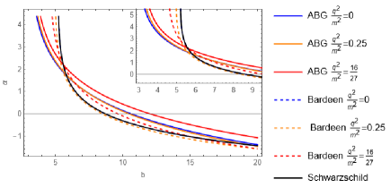
Figure 5: Comparison of light deflection for Regular Bardeen and Bardeen with ABG source

The calculated $\tilde{a}_{1}$ and $\tilde{a}_{2}$ are shown in Fig. 4. The $\tilde{a}_{1}$ slowly increases until $q=q_{crit}$ and then decreases linearly. The $\tilde{a}_{2}$, on the other hand, decreases as $q$ goes up until $q=q_{crit}$, then it starts increasing. The deflection angles are depicted in Fig. 5. It is shown that the critical impact parameters for the NLED models are smaller than for the pure Bardeen. This critical value increases with increasing charge.

V Lensing of Sgr A* as an ABG Black Hole

The most straightforward effect of light deflection due to gravitational field is the notion of “gravitational lensing”. The lensing mechanism can be inferred from Fig. 6. The straight segment $\overline{SO}$ is the path the light would have taken had it not been deflected due to the lens (BH) at $L$. The angle $\beta$ denotes the angular position of the source $S$ from the observer $O$ if there were no lensing. What the $O$ observes is the “image” of $S$ located at $I$ whose angular position is given by $\theta$. The deflection angle is given by $\alpha$. From simple geometry the relation between $\beta$ and $\theta$ can be expressed as Virbhadra:1999nm ; Bozza:2008ev

$$\tan\beta=\tan\theta-\frac{D_{LS}}{D_{OL}}\left[\tan\theta+\tan(\alpha-\theta)\right],$$ (38)

known as the lens equation.

In the strong field limit ($r_{0}\rightarrow r_{ps}$) $\beta$ and $\theta$ are small, $\alpha$ can exceed $2\pi$ and light can loop around the black hole several ($n$) times before escaping out to the observer.

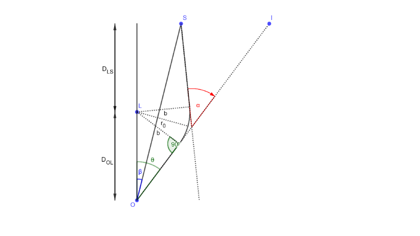
Figure 6: Gravitational lensing diagram. S, L, and O are the source, the lens, and the observer, respectively.

In this sense, $\alpha=2n\pi+\Delta\alpha_{n}$. We can then expand $\tan(\alpha-\theta)\sim\Delta\alpha_{n}-\theta$ Bozza:2001xd . The lens equation thus becomes

$$\beta=\theta-\frac{D_{LS}}{D_{OL}}\Delta\alpha_{n}.$$ (39)

We also have the relation

$$b=D_{OL}\theta.$$ (40)

Substituting it into (1) and inverting it results in Bozza:2002zj

$$\theta(\alpha)\simeq\frac{b_{c}}{D_{OL}}\left(1+e^{\frac{\tilde{a}_{2}-\alpha}{\tilde{a}_{1}}}\right).$$ (41)

From Fig. 6, the innermost image is given by

$$\theta_{\infty}=\frac{b_{c}}{D_{OL}}.$$ (42)

Expanding around $\alpha$ yields

$$\theta_{n}=\theta_{n}^{0}-\gamma_{n}\Delta\alpha_{n},$$ (43)

with

$$\theta_{n}^{0} = \frac{b_{c}}{D_{OL}}\left(1+e_{n}\right),$$ (44)

$$\gamma_{n} = \frac{b_{c}}{\tilde{a}_{2}D_{OL}}e_{n},$$ (45)

$$e_{n} = e^{\frac{\tilde{a}_{2}-2n\pi}{\tilde{a}_{1}}}.$$ (46)

We can eliminate $\Delta\alpha_{n}$ using the Eq. (39). This results in the equation for the n-th shadow position Bozza:2001xd ; Bozza:2002zj ; Tsukamoto:2016qro

$$\theta_{n}=\theta_{n}^{0}+\frac{D_{LS}}{D_{OS}}\gamma_{n}(\beta-\theta_{n}^{0}),$$ (47)

where the second term on the right-hand side is small compared to the first one. For the Einstein ring case, $\beta=0$ and

$$\theta_{nE}=\left(1-\frac{D_{LS}}{D_{OS}}\gamma_{n}\right)\theta_{n}^{0}.$$ (48)

The observables we wish to calculate are the image separation and the magnification. The separation $s$ is the difference between the outermost and innermost images,

$$s=\theta_{1}-\theta_{\infty}=\theta_{\infty}e^{\frac{\tilde{a}_{2}-2\pi}{\tilde{a}_{1}}}.$$ (49)

The magnification $\mu$ is the inverse of the corresponding Jacobian determinant for the critical curve schneider:1992 ; Bozza:2001xd . The $n^{th}$ image magnification is defined to be

$$\mu_{n}=\frac{1}{|\det J_{\theta_{n}^{0}}|}=\frac{1}{\frac{\beta}{\theta_{n}^{0}}\left.\frac{\partial\beta}{\partial\theta}\right|_{\theta_{n}^{0}}},$$ (50)

from which the (relativistic) flux ratio is expressed as

$$r=\frac{\mu_{1}}{\sum\limits_{n=2}^{\infty}\mu_{n}}=e^{\frac{2\pi}{\tilde{a}_{1}}}.$$ (51)

In this paper we calculate the strong lensing from the Sgr A* black hole modeled as the Bardeen with ABG source. We use data from GRAVITY collaboration where the black hole mass and its distance from the Earth (observer) are $m=4.154\times 10^{6}M_{\odot}$ and $D_{OL}=8.178\ kpc$, respectively abuterGeometricDistanceMeasurement2019 . These values are consistent with the EHT results EventHorizonTelescope:2022wkp . In Table 1 we show the observables. Here the value the magnification is converted to magnitudes $r_{m}=2.5\log_{10}r$ Bozza:2002zj . From the Table it can be seen that the observable values for the Bardeen does not differ much from that of RN. However, the observables for the ABG are significantly different from both Bardeen and RN; i.e., the ABG’s are smaller. This shows that the NLED effect is quite significant here.

Model	$Q/m$	$\theta_{\infty}$ ($\mu$ as)	$s$($\mu$ as)	$r_{m}$
Schwarzschild	-	26.0592	0.0327	6.8184
Bardeen	0	26.0592	0.0327	6.8184
	0.1	26.0156	0.0332351	6.79937
	0.2	25.8833	0.0349143	6.74083
	0.3	25.6569	0.0381989	6.63828
	0.4	25.3266	0.044135	6.48266
	0.5	24.8751	0.0552564	6.25695
	0.6	24.2718	0.0788401	5.92697
	0.7	23.4566	0.144124	5.41046
RN	0	26.0592	0.0327	6.8184
	0.1	26.0157	0.0330446	6.81081
	0.2	25.8841	0.0340718	6.7875
	0.3	25.6612	0.0359467	6.74699
	0.4	25.3412	0.0389696	6.68646
	0.5	24.9146	0.043696	6.60104
	0.6	24.3668	0.0511167	6.48246
	0.7	23.6747	0.0628463	6.31574
ABG	0	15.0453	1.01295	3.93662
	0.1	15.0593	1.015	3.93252
	0.2	15.1029	1.02079	3.92061
	0.3	15.1806	1.02911	3.90248
	0.4	15.3007	1.03751	3.88228
	0.5	15.4768	1.04185	3.87016
	0.6	15.7286	1.03655	3.8886
	0.7	16.0813	1.01629	3.9788

Table 1: Observables for the Sgr A* Schwarzschild, Bardeen, RN, and ABG. The $\theta$ and its corresponding separation are expressed in $\mu$ arc-second (as) unit.

From Table 1 it can be inferred that the ABG has $1.5\times$ smaller values of $\theta_{\infty}$ compared to Bardeen. This means that photon can orbit ABG with smaller radius. While the separation $s$ for the ABG is surprisingly $30\times$ larger, its magnification $r_{m}$ is smaller than for Bardeen. The NLED thus strengthens the gravitational field by decreasing the innermost distance while at the same time increasing its corresponding separation with the outermost image. Interestingly, the observables in the ABG behave in such opposite ways with the the ones in the Bardeen. In Figs. 7 it is shown that while the $\theta_{\infty}$ in Bardeen decreases monotonically, in the ABG case it increases.

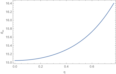
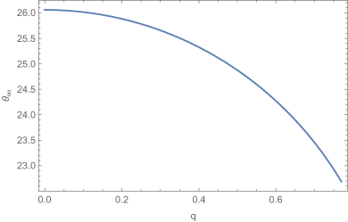
Figure 7: $\theta_{\infty}$ as function of $q$ for: [top] The ABG model and, [down] the original Bardeen.

From Figs. 8 the separation in the Bardeen model increases monotonically, while in the ABG there exists some maximum value $s=s_{max}$ before which it initially increases and after which it starts decreasing.

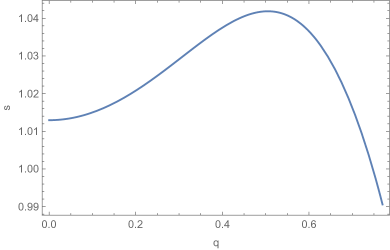
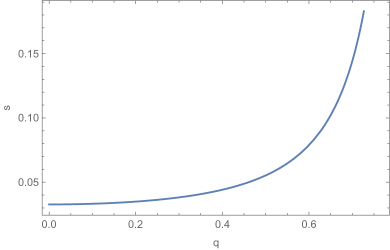
Figure 8: $s$ as function of $q$ for: [top] the ABG model, [down] the Bardeen model.

Similarly, in Figs. 9 we see that the $r_{m}$ decreases unboundedly for the Bardeen as $q$ increases, whereas it decreases to its minimum value before increasing monotonically for the ABG.

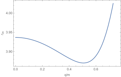
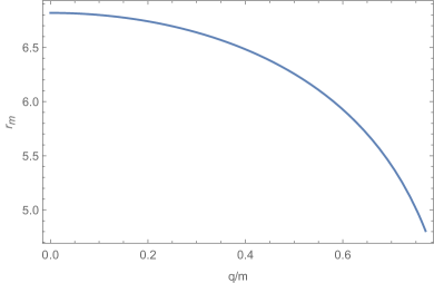
Figure 9: $r_{m}$ as function of $q$ for: [top] the ABG model, [down] the Bardeen model.

VI Is Sgr A* a nonsingular black hole?

Having calculated the lensing observables for the Sgr A* if its modeled as the ABG black hole, a tempting question would be: how realistic is Sgr A* as a nonsingular black hole? While to the best of our knowledge we have not found any strong lensing data of Sgr A* to compare with, we do have data for its shadow radius bound. The black hole shadow is the dark region surrounding it due to the inability of the photon from the background light source to escape the gravitational potential around the black hole. The size of the shadow corresponds to the critical impact parameter of the photon orbit Stuchlik:2019uvf ; Bisnovatyi-Kogan:2017kii ; Lu:2019zxb . The idea that the Sgr A* shadow can be observed was suggested in Falcke:1999pj ; Melia:2001dy ; Kruglov:2020tes . The shadow radius $R_{sh}$ is represented by the critical impact parameter, i.e., the impact parameter evaluated at the photon sphere radius $r_{ps}$ Cunha:2018acu ; Perlick:2021aok ,

$$R_{sh}=b_{c}=r_{ps}\sqrt{\frac{h(r_{ps})}{f(r_{ps})}}.$$ (52)

For Bardeen with ABG source we will have

$$R_{shABG}=r_{ps}\sqrt{\frac{\left(1-\frac{2(6q^{2}-r_{ps}^{2})}{(q^{2}+r_{ps}^{2})}\right)^{-1}}{\left(1-\frac{2mr_{ps}^{2}}{(r_{ps}^{2}+q^{2})^{3/2}}\right)}}.$$ (53)

Recently, Vagnozzi et al Vagnozzi:2022moj did a comprehensive horizon-scale test using the EHT data from the Sgr A* to constraint a wide range of classical black hole solutions. They calculate $\delta$, the fractional deviation between the inferred and and the Schwarzschild shadow radii, and compared them with the observational estimates by Keck and VLTI (Very Large Telescope Interferometer) EventHorizonTelescope:2022xqj :

$$\delta\simeq-0.060\pm 0.065.$$ (54)

Converting this bound into the shadow radius, and assuming Gaussian uncertainties, the constraint reads

$$4.54\lesssim R_{sh}/M\lesssim 5.22,$$ (55)

and

$$4.20\lesssim R_{sh}/M\lesssim 5.56,$$ (56)

for $1\sigma$ and $2\sigma$ levels, respectively.

Among the many BH solutions the authors of Ref. Vagnozzi:2022moj scrutinize, they left out the ABG BH unchecked. We plotted the shadow radius as a function of magnetic charge for the ABG BH in Eq. (53), , $R_{shABG}=R_{shABG}(q)$. The result is shown in Fig. 10. Interestingly, while the original Bardeen metric passes the horizon-scale test, Fig. (4) of Vagnozzi:2022moj , the effective metric of ABG does not, as can be seen from the figure. The radius shadow of ABG BH is way below the ETH constraint for Sgr A*. Thus, we conclude that the possibility of Sgr A* being an ABG black hole is ruled out.

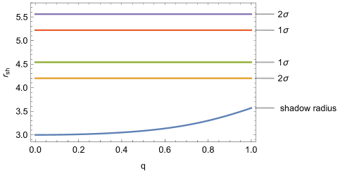
Figure 10: Shadow radius $r_{sh}$ of the ABG black hole as a function of magnetic charge $q$.

VII Conclusion

In this work, we study both the strong lensing and shadow phenomenology of nonsingular ABG black hole. Our approach is different either from Eiroa:2010wm ; Wei:2015qca in that we regard the nonsingularity coming from the NLED charge, or from Ghaffarnejad:2016dlw where we used simpler ABG NLED model.

The NLED reduces photon sphere radius with increasing $q$ until it reaches $q=q_{crit}$, after which it starts to increase monotonically. It also reduces the radius of the photon orbit, and also increases the gravitational field by pulling the innermost distance closer but at the same time stretching its separation distance from the outermost image. Our observable quantities behave differently from the ordinary Bardeen Eiroa:2010wm ; Wei:2015qca in terms of the innermost image (Figs. 7), the separation between innermost and outermost images (Figs. 8), and the magnification (Figs. 9). Interestingly, the NLED type that we particularly choose to model Bardeen in this paper gives distinct observable results compared to other types. While the model Ghaffarnejad:2016dlw predicts that the angular separation $s$ decreases while the magnification $r_{m}$ increases with increasing $q$, our results show the opposite. From Table 1 we can observe that as the charge increases, the angular separation does increase while the magnification does decrease.

Lastly, and more importantly, in this work we try to answer a tempting question of whether the Sgr A* at the center of our Milky Way is a nonsingular supermassive BH or not. Based on our shadow radius analysis, we show that Sgr A* cannot be the ABG black hole. Its shadow radius is way below the constraints imposed by EHT observational data. This is, however, is by no means saying that the Sgr A* cannot be nonsingular BH. In Ref. Vagnozzi:2022moj it is shown that the EHT observations are consistent with Sgr A* being a Hayward BH Hayward:2005gi . The static ABG model itself is non-realistic from astrophysical point of view for Sgr A*, since all black holes are supposed to be rotating. It would be interesting if we can put the rotating nonsingular black holes (for example, see Ghosh:2014pba ; Amir:2016cen ; Abdujabbarov:2016hnw ) to this horizon-scale test to see whether they are suitable to model the Sgr A*. Recently, Walia, Ghosh, and Maharaj tested the three rotating regular BHs (Hayward, Bardeen, and Simpson-Visser) using the EHT observations for Sgr A* KumarWalia:2022aop . They concluded that those three metrics can be still within the EHT bounds and thus the possibility of Sgr A* being one of them cannot be ruled out. However, their black hole metrics are not sourced by the NLED charge. Due to the rotating nature, it is not known whether such exact solutions exist for coupled Einstein-NLED equations.

Data Availability Statement

Data sharing is not applicable to this article as no data sets were generated or analyzed during the current study.

References

- (1) K. Akiyama et al. [Event Horizon Telescope], “First M87 Event Horizon Telescope Results. I. The Shadow of the Supermassive Black Hole,” Astrophys. J. Lett. 875 (2019), L1 [arXiv:1906.11238 [astro-ph.GA]].
- (2) K. Akiyama et al. [Event Horizon Telescope], “First Sagittarius A* Event Horizon Telescope Results. I. The Shadow of the Supermassive Black Hole in the Center of the Milky Way,” Astrophys. J. Lett. 930 (2022) no.2, L12
- (3) H. Falcke, F. Melia and E. Agol, “Viewing the shadow of the black hole at the galactic center,” Astrophys. J. Lett. 528 (2000), L13 [arXiv:astro-ph/9912263 [astro-ph]].
- (4) Schneider, P., Ehlers, J. & Falco, E. Gravitational Lenses. “Gravitational Lenses.” (1992)
- (5) V. Perlick, “Gravitational lensing from a spacetime perspective,” Living Rev. Rel. 7 (2004), 9
- (6) C. Darwin, “The gravity field of a particle,” Proceedings Of The Royal Society Of London. Series A. Mathematical And Physical Sciences. 249.
- (7) V. Bozza, “Gravitational Lensing by Black Holes,” Gen. Rel. Grav. 42 (2010), 2269-2300 [arXiv:0911.2187 [gr-qc]].
- (8) J. P. Luminet, “Image of a spherical black hole with thin accretion disk,” Astron. Astrophys. 75 (1979), 228-235
- (9) A. Chowdhuri, S. Ghosh and A. Bhattacharyya, “A review on analytical studies in Gravitational Lensing,” Front. Phys. 11 (2023), 1113909 [arXiv:2303.02069 [gr-qc]].
- (10) S. Ghosh and A. Bhattacharyya, “Analytical study of gravitational lensing in Kerr-Newman black-bounce spacetime,” JCAP 11 (2022), 006 [arXiv:2206.09954 [gr-qc]].
- (11) S. Chandrasekhar, “The mathematical theory of black holes,”
- (12) S. Frittelli, T. P. Kling and E. T. Newman, Phys. Rev. D 61 (2000), 064021 [arXiv:gr-qc/0001037 [gr-qc]].
- (13) K. S. Virbhadra and G. F. R. Ellis, “Schwarzschild black hole lensing,” Phys. Rev. D 62 (2000), 084003 [arXiv:astro-ph/9904193 [astro-ph]].
- (14) V. Bozza, S. Capozziello, G. Iovane and G. Scarpetta, “Strong field limit of black hole gravitational lensing,” Gen. Rel. Grav. 33 (2001), 1535-1548 [arXiv:gr-qc/0102068 [gr-qc]].
- (15) V. Bozza, “Gravitational lensing in the strong field limit,” Phys. Rev. D 66 (2002), 103001 [arXiv:gr-qc/0208075 [gr-qc]].
- (16) K. S. Virbhadra, “Distortions of images of Schwarzschild lensing,” Phys. Rev. D 106 (2022) no.6, 064038 [arXiv:2204.01879 [gr-qc]].
- (17) N. Tsukamoto, “Strong deflection limit analysis and gravitational lensing of an Ellis wormhole,” Phys. Rev. D 94 (2016) no.12, 124001 [arXiv:1607.07022 [gr-qc]].
- (18) N. Tsukamoto, “Deflection angle in the strong deflection limit in a general asymptotically flat, static, spherically symmetric spacetime,” Phys. Rev. D 95 (2017) no.6, 064035 [arXiv:1612.08251 [gr-qc]].
- (19) E. F. Eiroa, G. E. Romero and D. F. Torres, “Reissner-Nordstrom black hole lensing,” Phys. Rev. D 66 (2002), 024010 [arXiv:gr-qc/0203049 [gr-qc]].
- (20) V. Bozza, “Quasiequatorial gravitational lensing by spinning black holes in the strong field limit,” Phys. Rev. D 67 (2003), 103006 [arXiv:gr-qc/0210109 [gr-qc]].
- (21) S. E. Vazquez and E. P. Esteban, “Strong field gravitational lensing by a Kerr black hole,” Nuovo Cim. B 119 (2004), 489-519 [arXiv:gr-qc/0308023 [gr-qc]].
- (22) V. Bozza, F. De Luca and G. Scarpetta, “Kerr black hole lensing for generic observers in the strong deflection limit,” Phys. Rev. D 74 (2006), 063001 [arXiv:gr-qc/0604093 [gr-qc]].
- (23) J. R. Oppenheimer and H. Snyder, “On Continued gravitational contraction,” Phys. Rev. 56 (1939), 455-459
- (24) R. Penrose, “Gravitational collapse and space-time singularities,” Phys. Rev. Lett. 14 (1965), 57-59
- (25) J. Bardeen, “Non-Singular General-Relativistic Gravitational Collapse,” Proc. Int. Conf. GR5, Tbilisi 174 (1968).
- (26) S. Ansoldi, “Spherical black holes with regular center: A Review of existing models including a recent realization with Gaussian sources,” [arXiv:0802.0330 [gr-qc]].
- (27) E. F. Eiroa and C. M. Sendra, “Gravitational lensing by a regular black hole,” Class. Quant. Grav. 28 (2011), 085008 [arXiv:1011.2455 [gr-qc]].
- (28) S. W. Wei, Y. X. Liu and C. E. Fu, “Null Geodesics and Gravitational Lensing in a Nonsingular Spacetime,” Adv. High Energy Phys. 2015 (2015), 454217 [arXiv:1510.02560 [gr-qc]].
- (29) E. Ayon-Beato and A. Garcia, “Regular black hole in general relativity coupled to nonlinear electrodynamics,” Phys. Rev. Lett. 80 (1998), 5056-5059 [arXiv:gr-qc/9911046 [gr-qc]].
- (30) E. Ayon-Beato and A. Garcia, “The Bardeen model as a nonlinear magnetic monopole,” Phys. Lett. B 493 (2000), 149-152 [arXiv:gr-qc/0009077 [gr-qc]].
- (31) Novello, M., De Lorenci, V., Salim, J. & Klippert, R. Geometrical aspects of light propagation in nonlinear electrodynamics. Phys. Rev. D. 61 pp. 045001 (2000)
- (32) A. Allahyari, M. Khodadi, S. Vagnozzi and D. F. Mota, “Magnetically charged black holes from non-linear electrodynamics and the Event Horizon Telescope,” JCAP 02 (2020), 003
- (33) H. Ghaffarnejad, M. Amirmojahedi and H. Niad, “Gravitational Lensing of Charged Ayon-Beato-Garcia Black Holes and Nonlinear Effects of Maxwell Fields,” Adv. High Energy Phys. 2018 (2018), 3067272 doi:10.1155/2018/3067272 [arXiv:1601.05749 [physics.gen-ph]].
- (34) S. Weinberg, “Gravitation and Cosmology: Principles and Applications of the General Theory of Relativity,” John Wiley and Sons, 1972, ISBN 978-0-471-92567-5, 978-0-471-92567-5
- (35) V. Bozza, “A Comparison of approximate gravitational lens equations and a proposal for an improved new one,” Phys. Rev. D 78 (2008), 103005 [arXiv:0807.3872 [gr-qc]].
- (36) The GRAVITY Collaboration, “A geometric distance measurement to the galactic center black hole with 0.3% uncertainty,” Astron. Astrophys. 625 (2019), L 10.
- (37) Z. Stuchlík and J. Schee, “Shadow of the regular Bardeen black holes and comparison of the motion of photons and neutrinos,” Eur. Phys. J. C 79 (2019) no.1, 44
- (38) G. S. Bisnovatyi-Kogan and O. Y. Tsupko, “Gravitational Lensing in Presence of Plasma: Strong Lens Systems, Black Hole Lensing and Shadow,” Universe 3 (2017) no.3, 57 [arXiv:1905.06615 [gr-qc]].
- (39) H. Lu and H. D. Lyu, “Schwarzschild black holes have the largest size,” Phys. Rev. D 101 (2020) no.4, 044059 [arXiv:1911.02019 [gr-qc]].
- (40) F. Melia and H. Falcke, “The supermassive black hole at the galactic center,” Ann. Rev. Astron. Astrophys. 39 (2001), 309-352 [arXiv:astro-ph/0106162 [astro-ph]].
- (41) S. I. Kruglov, “The shadow of M87* black hole within rational nonlinear electrodynamics,” Mod. Phys. Lett. A 35 (2020) no.35, 2050291 [arXiv:2009.07657 [gr-qc]].
- (42) P. V. P. Cunha and C. A. R. Herdeiro, “Shadows and strong gravitational lensing: a brief review,” Gen. Rel. Grav. 50 (2018) no.4, 42.
- (43) V. Perlick and O. Y. Tsupko, “Calculating black hole shadows: Review of analytical studies,” Phys. Rept. 947 (2022), 1-39.
- (44) S. Vagnozzi, R. Roy, Y. D. Tsai, L. Visinelli, M. Afrin, A. Allahyari, P. Bambhaniya, D. Dey, S. G. Ghosh and P. S. Joshi, et al. “Horizon-scale tests of gravity theories and fundamental physics from the Event Horizon Telescope image of Sagittarius A∗,” [arXiv:2205.07787 [gr-qc]].
- (45) K. Akiyama et al. [Event Horizon Telescope], “First Sagittarius A* Event Horizon Telescope Results. VI. Testing the Black Hole Metric,” Astrophys. J. Lett. 930 (2022) no.2, L17
- (46) S. A. Hayward, “Formation and evaporation of regular black holes,” Phys. Rev. Lett. 96 (2006), 031103 [arXiv:gr-qc/0506126 [gr-qc]].
- (47) S. G. Ghosh, “A nonsingular rotating black hole,” Eur. Phys. J. C 75 (2015) no.11, 532 [arXiv:1408.5668 [gr-qc]].
- (48) M. Amir and S. G. Ghosh, “Shapes of rotating nonsingular black hole shadows,” Phys. Rev. D 94 (2016) no.2, 024054 [arXiv:1603.06382 [gr-qc]].
- (49) A. Abdujabbarov, M. Amir, B. Ahmedov and S. G. Ghosh, “Shadow of rotating regular black holes,” Phys. Rev. D 93 (2016) no.10, 104004 [arXiv:1604.03809 [gr-qc]].
- (50) R. Kumar Walia, S. G. Ghosh and S. D. Maharaj, “Testing Rotating Regular Metrics with EHT Results of Sgr A*,” Astrophys. J. 939 (2022) no.2, 77 [arXiv:2207.00078 [gr-qc]].