M²SNet: Multi-scale in Multi-scale Subtraction Network for Medical Image Segmentation

Abstract

Accurate medical image segmentation is critical for early medical diagnosis. Most existing methods are based on U-shape structure and use element-wise addition or concatenation to fuse different level features progressively in decoder. However, both the two operations easily generate plenty of redundant information, which will weaken the complementarity between different level features, resulting in inaccurate localization and blurred edges of lesions. To address this challenge, we propose a general multi-scale in multi-scale subtraction network (M²SNet) to finish diverse segmentation from medical image. Specifically, we first design a basic subtraction unit (SU) to produce the difference features between adjacent levels in encoder. Next, we expand the single-scale SU to the intra-layer multi-scale SU, which can provide the decoder with both pixel-level and structure-level difference information. Then, we pyramidally equip the multi-scale SUs at different levels with varying receptive fields, thereby achieving the inter-layer multi-scale feature aggregation and obtaining rich multi-scale difference information. In addition, we build a training-free network “LossNet” to comprehensively supervise the task-aware features from bottom layer to top layer, which drives our multi-scale subtraction network to capture the detailed and structural cues simultaneously. Without bells and whistles, our method performs favorably against most state-of-the-art methods under different evaluation metrics on eleven datasets of four different medical image segmentation tasks of diverse image modalities, including color colonoscopy imaging, ultrasound imaging, computed tomography (CT), and optical coherence tomography (OCT). The source code can be available at https://github.com/Xiaoqi-Zhao-DLUT/MSNet.

Medical Image Segmentation, Subtraction Unit, Multi-scale in Multi-scale, Difference Information, LossNet.

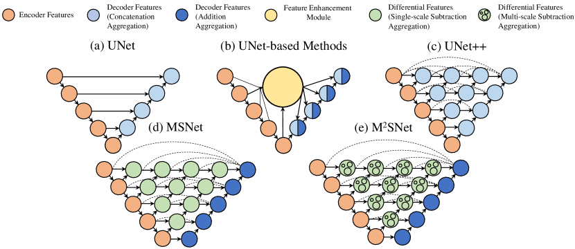
Figure 1: Illustration of different medical image segmentation architectures.

1 Introduction

As the important role in computer-aided diagnosis system, accurate medical image segmentation technique can provide the doctors with great guidance for making clinical decisions. There are three general challenges in accurate segmentation: Firstly, U-shape structures [1, 2] have received considerable attention due to their abilities of utilizing multi-level information to reconstruct high-resolution feature maps. In UNet [2], the up-sampled feature maps are concatenated with feature maps skipped from the encoder and convolutions and non-linearities are added between up-sampling steps, as shown in Fig. 1 (a). Subsequent UNet-based methods design diverse feature enhancement modules via attention mechanism [3, 4], gate mechanism [5, 6], transformer technique [7, 8], as shown in Fig. 1 (b). UNet++ [9] uses nested and dense skip connections to reduce the semantic gap between the feature maps of encoder and decoder, as shown in Fig. 1 (c). Generally speaking, different level features in encoder have different characteristics. High-level ones have more semantic information which helps localize the objects, while low-level ones have more detailed information which can capture the subtle boundaries of objects. The decoder leverages the level-specific and cross-level characteristics to generate the final high-resolution prediction. Nevertheless, the aforementioned methods directly use an element-wise addition or concatenation to fuse any two level features from the encoder and transmit them to the decoder. These simple operations do not pay more attention to differential information between different levels. This drawback not only generates redundant information to dilute the really useful features but also weakens the characteristics of level-specific features, which results in that the network can not balance accurate localization and subtle boundary refinement. Secondly, due to the limited receptive field, a single-scale convolutional kernel is difficult to capture context information of size-varying objects. Some methods [1, 2, 9, 10, 11] rely on the inter-layer multi-scale features and progressively integrate the semantic context and texture details from diverse scale representations. Others [6, 12, 13, 14, 15] focus on extracting the intra-layer multi-scale information based on the atrous spatial pyramid pooling module [16] (ASPP) or DenseASPP [17] in their networks. However, the ASPP-like multi-scale convolution modules will produce many extra parameters and computations. Many methods [5, 18, 19, 20, 21] usually equip several ASPP modules into the encoder/decoder blocks of different levels, while some ones [13, 22, 14, 23] install it on the highest-level encoder block. Thirdly, the form of the loss function directly provides the direction for the gradient optimization of the network. In segmentation field, there are many loss functions are proposed to supervise the prediction at the different levels, such as the L1 loss, cross-entropy loss and weighted cross-entropy loss [24] in the pixel level, the SSIM [25] loss and uncertainty-aware loss [26] in the region level, the IoU loss, Dice loss and consistency-enhanced loss [11] in the global level. Although these basic loss functions and their variants have different optimization characteristics, the designs of complex manual math forms are really time-consuming for many researches. In order to obtain comprehensive performance, models usually integrate a variety of loss functions, which places great demands on the training skills of the researchers. Therefore, we think that it is necessary to introduce an intelligent loss function without complex manual designs to comprehensively supervise the segmentation prediction.

In this paper, we propose a novel multi-scale in multi-scale subtraction network (M²SNet) for general medical image segmentation. Firstly, we design a subtraction unit (SU) and apply it to each pair of adjacent level features. The SU highlights the useful difference information between the features and eliminates the interference from the redundant parts. Secondly, we collect the extreme multi-scale information with the help of the proposed multi-scale in multi-scale subtraction module. For the inter-layer multi-scale information, we pyramidally concatenate multiple subtraction units to capture the large-span cross-level information. Then, we aggregate level-specific features and multi-path cross-level differential features and then generate the final prediction in decoder. For the intra-layer multi-scale information, we improve the single-scale subtraction unit to the multi-scale subtraction unit through a group of full one filters with different kernel sizes, which can achieve naturally multi-scale subtraction aggregation without introducing extra parameters. As shown in Fig. 1, MSNet equips the inter-layer multi-scale subtraction module and M²SNet has both the inter-layer and intra-layer multi-scale subtraction structures. Thirdly, we propose a LossNet to automatically supervise the extracted feature maps from bottom layer to top layer, which can optimize the segmentation from detail to structure with a simple L2-loss function.

Our main contributions are summarized as follows:

• We present a new segmentation framework by replacing traditional addition or concatenation feature fusion with an efficient subtraction aggregation.

• We propose a simple yet general multi-scale in multi-scale subtraction network (M²SNet) for diverse medical image segmentation. With multi-scale in multi-scale module, the multi-scale complementary information from lower order to higher order among different levels can be effectively obtained, thereby comprehensively enhancing the perception of organs or lesion areas.

• We design an efficient intra-layer multi-scale subtraction unit (MSU). Due to the low parameters and computation of MSU, it can be equipped for all cross-layer aggregations in our M²SNet.

• We build a general training-free loss network to implement the detail-to-structure supervision in the feature levels, which provides the important supplement to the loss design based on the prediction itself.

• We verify the effectiveness of the M²SNet on four challenge medical segmentation tasks: polyp segmentation, breast cancer segmentation, COVID-19 lung infection and OCT layer segmentation corresponding to the color colonoscopy imaging, ultrasound imaging, computed tomography (CT), and optical coherence tomography (OCT) image input modality, respectively. In addition, M²SNet won the second place in the MICCAI2022 GOALS International Ophthalmology Challenge.

Compared with the MICCAI version [27] of this work, the following extensions are made. I) Based on the structure of the original single-scale subtraction unit, we develop the stronger intra-layer multi-subtraction unit and construct the multi-scale in multi-scale subtraction network (M²SNet). Meanwhile, M²SNet carries forward the low FLOPs spirit of the previous MSNet. II) We re-organize the introduction and add more thorough related works in Sec. 2. III) We report much more extensive experimental results that demonstrate the superiority of M²SNet in $4$ popular medical segmentation tasks. IV) We verify the performance of the M²SNet for multi-class segmentation in the MICCAI 2022 Challenge: Glaucoma Oct Analysis and Layer Segmentation (GOALS). We won the second place (2/100). V) We further provide more implementation details and thorough ablation studies at qualitative and quantitative aspects. VI) We perform in-depth analyses and discussions for our multi-scale subtraction unit.

2 Related Work

2.1 Medical Image Segmentation Network

According to the characteristics of different organs or lesions, we classify existing medical image segmentation methods into two types: medical-general and medical-specific one.
Medicine-general Methods. With the U-Net [2] achieving stable performance in the medical image segmentation field, the U-shape structure with encoder-decoder has become the basic segmentation baseline. U-Net++ [9] integrates both the long connection and short connection, which can reduce the semantic gap between the feature maps of the encoder and decoder sub-networks. For attention U-Net [28], an attention gate is embedded in each transition layer between the encoder and decoder block, which can automatically learn to focus on target structures of varying shapes and sizes. Recently, the Transformer [29] architecture has achieved success in many natural language processing tasks. Some works [7, 8] explore its effectiveness for the medical vision tasks. UTNet [7] is a simple but powerful hybrid transformer architecture, which applies the self-attention module in both the encoder and decoder to capture remote dependencies of different scales with minimal overhead. Another representative transformer-based model is the TransUNet [8], which encodes strong global context by treating the image features as sequences and utilizes the low-level CNN features via a u-shaped hybrid architectural design.
Medicine-specific Methods. In the polyp segmentation task, SFA [30] and PraNet [4], focus on recovering the sharp boundary between a polyp and its surrounding mucosa. The former proposes a selective feature aggregation structure and a boundary-sensitive loss function under a shared encoder and two mutually constrained decoders. The latter utilizes a reverse attention module to establish the relationship between the region and boundary cues. In addition, Ji et al. [31] utilize spatio-temporal information to build the video polyp segmentation model. In the COVID-19 lung infection task, Paluru et al. [32] propose an anamorphic depth embedding-based lightweight CNN to segment anomalies in COVID-19 chest CT images. Inf-Net [33] builds the implicit reverse attention and explicit edge attention to model the boundaries. BCS-Net [34] has three progressive boundary context-semantic reconstruction blocks, which can help the decoder to capture the piecemeal region for lung infection. In the breast segmentation task, Byra et al. [35] develop a selective kernel via an attention mechanism to adjust the receptive fields of the U-Net, which can further improve the segmentation accuracy of breast tumors. Chen et al. [36] propose a nested U-net to achieve robust representation of breast tumors by exploiting different depths and sharing weights.

We can see that the medicine-general methods are usually towards general challenges (i.e., rich feature representation, multi-scale information extraction and cross-level feature aggregation). And, the medicine-specific methods propose targeted solutions based on the characteristics of the current organ or lesion, such as designing a series of attention mechanisms, edge enhancement modules, uncertainty estimation, etc. However, both general medicine-general and medicine-specific models rely on a large number of addition or concatenation operations to achieve feature fusion, which weakens the specificity parts among complementary features. Our proposed multi-scale subtraction module naturally focuses on extracting difference information, thus providing the decoder with efficient targeted features.

2.2 Multi-scale Feature Extraction

Scale cues play an important role in capturing contextual information of objects. Inspired by the scale-space theory that has been widely validated as an effective and theoretically sound framework, more and more multi-scale methods are proposed. Compared with single-scale features, multi-scale features are beneficial to address naturally occurring scale variations. This characteristic can help the medical segmentation models perceive lesions with different scales. According to the form, current multi-scale based methods can be roughly divided into two categories, namely, the inter-layer multi-scale structure and the intra-layer multi-scale structure. The former is based on features with different scales extracted by the feature encoder and progressively aggregates them in decoder, such as the U-shape [2, 9, 1, 37, 4, 10, 38, 11] architecture. The latter usually equips the multi-scale pluggable modules, such as ASPP [16], DenseASPP [17], FoldASPP [6], and PAFEM [12] to construct the parallel multi-branch convolution layers with different dilated rates to obtain a rich combination of receptive fields. Different from them, we propose the multi-scale in multi-scale subtraction module with the extreme multi-scale information through introducing both inter-layer and intra-layer multi-scale at once. And, the intra-layer multi-scale subtraction unit focuses on mining the self-difference properties of the pairs of features from pixel-pixel to region-region. The whole process is very efficient without extra parameters compared to single-scale operations.

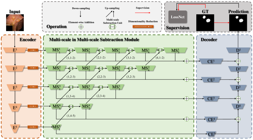
Figure 2: Overview of the proposed multi-scale subtraction network.

2.3 Loss Method

Most loss functions in image segmentation are based on cross-entropy or coincidence measures. The traditional cross-entropy loss treats the categories information equally. Long et al. [24] propose a weighted cross-entropy loss (WCE) for each class to offset the class imbalance in the data. Lin et al. [39] introduce the weights of difficult and easy samples to propose the Focal loss. Dice loss [40] is proposed as the loss function of coincidence measurement in V-Net, which can effectively suppress problems caused by category imbalance. Tversky loss [41] is a regularized version of Dice loss to control the contribution of accuracy and recall to the loss function. Wong et al. [42] propose exponential logarithmic loss (EL Loss) through the weighted summation of Dice loss and WCE loss to improve the segmentation accuracy of small structure objects. Taghanaki et al. [43] find that there is a risk in using the loss function based on overlap alone, and propose the como-loss to combine Dice loss as a regularization term with WCE loss to deal with the problem of input and output imbalance. Although these various loss functions have different effects at different levels, it is indeed time-consuming and laborious to manually design these complex functions. To this end, we propose the automatic and comprehensive segmentation loss structure, coined as the LossNet.

3 Method

The M²SNet architecture is shown in Fig. 2, in which there are five encoder blocks ($\mathbf{E}^{i}$, $i\in\left\{1,2,3,4,5\right\}$), a multi-scale in multi-scale subtraction module (MMSM) and four decoder blocks ($\mathbf{D}^{i}$, $i\in\left\{1,2,3,4\right\}$). We adopt the Res2Net-50 as the backbone to extract five levels of features. First, we separately adopt a $3\times 3$ convolution for feature maps of each encoder block to reduce the channel to $64$, which can decrease the number of parameters for subsequent operations. Next, these different level features are fed into the MMSM and output five complementarity enhanced features (${CE}^{i}$, $i\in\left\{1,2,3,4,5\right\}$). Finally, each ${CE}^{i}$ progressively participates in the decoder and generates the final prediction. In the training phase, both the prediction and ground truth are input into the LossNet to achieve supervision. We describe the multi-scale in multi-scale subtraction module in Sec. 3.1 and give the details of LossNet in Sec. 3.2.

3.1 Multi-scale in Multi-scale Subtraction Module

We use $F_{A}$ and $F_{B}$ to represent adjacent level feature maps. They all have been activated by the ReLU operation. We define a basic subtraction unit (SU):

$$\begin{split}SU=Conv(|F_{A}\ominus F_{B}|),\end{split}$$ (1)

where $\ominus$ is the element-wise subtraction operation, $|\cdot|$ calculates the absolute value and $Conv(\cdot)$ denotes the convolution layer. Directly performing single-scale subtraction on the features of element positions is only to establish the difference relationship on the isolated pixel level, without considering that the lesion may have the characteristics of regional clustering. Compared to the MICCAI version [27] of MSNet with the single-scale subtraction unit, we design a powerful intra-layer multi-scale subtraction unit (MSU) and improve MSNet to M²SNet. As shown in Fig. 3, we utilize the multi-scale convolution filters with fixed full one weights of size $1\times 1$, $3\times 3$ and $5\times 5$ to calculate the detail and structure difference values according to the pixel-pixel and region-region pattern. Using multi-scale filters with fixed parameters not only can directly capture the multi-scale difference clues between initial feature pairs at matched spatial locations, but also achieve efficient training without introducing additional parameter burdens. Therefore, M²SNet can maintain the same low computation as MSNet and achieve higher precision performance. The entire multi-scale subtraction process can be formulated as:

$$\begin{split}MSU=Conv(\quad\quad\quad\quad\quad\quad\\ |Filter(F_{A})_{1\times 1}\ominus Filter(F_{B})_{1\times 1}|+\\ |Filter(F_{A})_{3\times 3}\ominus Filter(F_{B})_{3\times 3}|+\\ |Filter(F_{A})_{5\times 5}\ominus Filter(F_{B})_{5\times 5}|),\end{split}$$ (2)

where $Filter(\cdot)_{n\times n}$ represents the full one filter of size $n\times n$. The MSU can capture the complementary information of $F_{A}$ and $F_{B}$ and highlight their differences from texture to structure, thereby providing richer information for the decoder.

To obtain higher-order complementary information across multiple feature levels, we horizontally and vertically concatenate multiple MSUs to calculate a series of differential features with different orders and receptive fields. The detail of the multi-scale in multi-scale subtraction module can be found in Fig. 2. We aggregate the scale-specific feature ($MS^{i}_{1}$) and cross-scale differential features ($MS^{i}_{n\neq 1}$) between the corresponding level and any other levels to generate complementarity enhanced feature ($CE^{i}$). This process can be formulated as follows:

$$\begin{split}CE^{i}=Conv(\sum_{n=1}^{6-i}MS^{i}_{n})\quad i=1,2,3,4,5.\end{split}$$ (3)

Finally, all $CE^{i}$ participate in decoding and then the polyp region is segmented.

3.2 LossNet

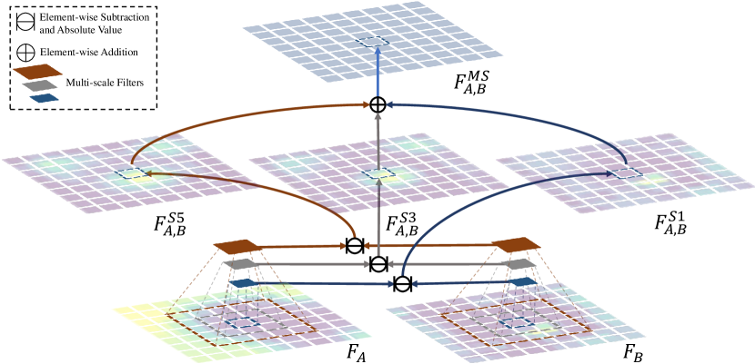
Figure 3: Detailed diagram of multi-scale subtraction unit.

In the proposed model, the total training loss can be written as:

$$\begin{split}\mathcal{L}_{total}=\mathcal{L}_{IoU}^{w}+\mathcal{L}_{BCE}^{w}+\mathcal{L}_{f},\end{split}$$ (4)

where $\mathcal{L}_{IoU}^{w}$ and $\mathcal{L}_{BCE}^{w}$ represent the weighted IoU loss and binary cross-entropy (BCE) loss which have been widely adopted in segmentation tasks. We use the same definitions as in  [4, 44, 45] and their effectiveness has been validated in these works. Different from them, we extra use a LossNet to further optimize the segmentation from detail to structure. Specifically, we use an ImageNet pre-trained classification network, such as VGG-16, to extract the multi-scale features of the prediction and ground truth, respectively. Then, their feature difference is computed as loss $\mathcal{L}_{f}$:

$$\begin{split}\mathcal{L}_{f}={l}_{f}^{1}+{l}_{f}^{2}+{l}_{f}^{3}+{l}_{f}^{4}.\end{split}$$ (5)

Let ${F}_{P}^{i}$ and ${F}_{G}^{i}$ separately represent the $i$-th level feature maps extracted from the prediction and ground truth. The ${l}_{f}^{i}$ is calculated as their Euclidean distance (L2-Loss), which is supervised at the pixel level:

$$\begin{split}{l}_{f}^{i}=||{F}_{P}^{i}-{F}_{G}^{i}||_{2},\quad i=1,2,3,4.\end{split}$$ (6)

As can be seen from Fig 4, the low-level feature maps contain rich boundary information and the high-level ones depict location information. Thus, the LossNet can generate comprehensive supervision at the feature levels.

Figure 4: Illustration of LossNet.

4 Experiments

4.1 Datasets

Extensive experiments are conducted to verify the effectiveness of the proposed framework on four different types of medical segmentation tasks with data from varied image modalities, including color colonoscopy imaging, ultrasound imaging, computed tomography (CT), and optical coherence tomography (OCT).

Polyp Segmentation. According to GLOBOCAN 2020 data, colorectal cancer is the third most common cancer worldwide and the second most common cause of death. It usually begins as small, noncancerous (benign) clumps of cells called polyps that form on the inside of the colon. We evaluate the proposed model on five benchmark datasets: CVC-ColonDB [46], ETIS [47], Kvasir [48], CVC-T [49] and CVC-ClinicDB [50]. We adopt the same training set as the latest image polyp segmentation method [4], that is, $900$ samples from the Kvasir and $550$ samples from the CVC-ClinicDB [50] are used for training. The remaining images and the other three datasets are used for testing. Besides, there are some video-based polyp datasets, including the CVC-300[51] and CVC-612[50]. We follow the latest video polyp segmentation method to split the videos from CVC-300 (12 clips) and CVC-612 (29 clips) into 60% for training, 20% for validation, and 20% for testing.

COVID-19 Lung Infection. Coronavirus Disease 2019 (COVID-19) spread globally in early 2020, causing the world to face an existential health crisis. At present, there are few public COVID-19 lung CT datasets for infection segmentation. To have relatively sufficient samples for training, we slice the public dataset [52] and merge with the public datasets [53] to obtain $1,277$ high-quality CT images by uniform sampling. And then, we further divide them into $894$ training images and $383$ testing images.

Breast Ultrasound Segmentation. Breast cancer is one of the most dreaded cancers in women [54]. Segmenting the lesion region from breast ultrasound images is essential for tumor diagnosis. BUSI [55] dataset contains $780$ images of $600$ female patients. Among them, there are $133$ normal cases, $437$ benign tumors, and $210$ malignant tumors. We follow the popular breast ultrasound segmentation methods [35, 36] to perform four-fold cross-validation on BUSI.

OCT Layer Segmentation. The OCT images are often used to diagnose and monitor retinal diseases more accurately based on abnormality quantification and retinal layer thickness computation both in research centers and clinic routines. At present, many scholars have been studying the segmentation of fundus structure in macular OCT scans, but few focus on parapapillary circular scans. To fully show the generalization of M²SNet in different medical tasks, we take our M²SNet to participate in MICCAI 2022 Challenge: Glaucoma Oct Analysis and Layer Segmentation (GOALS). It requests participants to segment three layers, which has positive significance for the diagnosis of glaucoma, including retinal nerve fiber layer (RNFL), ganglion cell-inner plexiform layer (GCIPL), and choroid layer, as shown in Fig. 5. The GOALS2022 [56] dataset contains $300$ circumpapillary OCT. There are three equal groups with $100$ OCT images for the training process, the preliminary competition process and the final process, respectively. The GOALS2022 challenge attracts $100$ teams from all over the world to participate, and we finally won the second place (2/100).

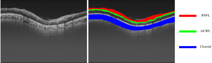
Figure 5: Visualization of the fundus OCT layer segmentation.

Table 1: Quantitative comparisons on image polyp segmentation datasets. Top $2$ scores are highlighted in red and blue, respectively. “$\dagger$” represents the medicine-specific method.

	Methods	Backbone	mDice $\uparrow$	mIoU $\uparrow$	$F_{\beta}^{w}$ $\uparrow$	$S_{\alpha}$ $\uparrow$	$E_{\phi}^{max}$ $\uparrow$	MAE $\downarrow$
ColonDB	U-Net [2]	R2-50	0.519	0.449	0.498	0.711	0.763	0.061
	U-Net++ [9]	R2-50	0.490	0.413	0.467	0.691	0.762	0.064
	Atten-UNet [28]	R2-50	0.466	0.385	0.431	0.670	0.724	0.071
	UTNet [7]	R-50 + ViT-B16	0.676	0.600	0.656	0.799	0.855	0.041
	TransUnet [8]	R-50 + ViT-B16	0.717	0.645	0.685	0.824	0.841	0.044
	SFA† [30]	R2-50	0.467	0.351	0.379	0.634	0.648	0.094
	PraNet† [4]	R2-50	0.716	0.645	0.699	0.820	0.847	0.043
	MSNet [27]	R2-50	0.755	0.678	0.737	0.836	0.883	0.041
	M2SNet	R2-50	0.758	0.685	0.737	0.842	0.869	0.038
ETIS	U-Net [2]	R2-50	0.406	0.343	0.366	0.682	0.645	0.036
	U-Net++ [9]	R2-50	0.413	0.342	0.390	0.681	0.704	0.035
	Atten-UNet [28]	R2-50	0.382	0.308	0.372	0.641	0.670	0.050
	UTNet [7]	R-50 + ViT-B16	0.556	0.489	0.522	0.749	0.772	0.022
	TransUNet [8]	R-50 + ViT-B16	0.573	0.512	0.517	0.765	0.707	0.029
	SFA† [30]	R2-50	0.297	0.219	0.231	0.557	0.515	0.109
	PraNet† [4]	R2-50	0.630	0.576	0.600	0.791	0.792	0.031
	MSNet [27]	R2-50	0.719	0.664	0.678	0.840	0.830	0.020
	M2SNet	R2-50	0.749	0.678	0.712	0.846	0.872	0.017
Kvasir	U-Net [2]	R2-50	0.821	0.756	0.794	0.858	0.901	0.055
	U-Net++ [9]	R2-50	0.824	0.753	0.808	0.862	0.907	0.048
	Atten-UNet [28]	R2-50	0.769	0.683	0.730	0.828	0.859	0.062
	UTNet [7]	R-50 + ViT-B16	0.862	0.803	0.843	0.886	0.911	0.042
	TransUNet [8]	R-50 + ViT-B16	0.869	0.816	0.847	0.899	0.920	0.040
	SFA† [30]	R2-50	0.725	0.619	0.670	0.782	0.828	0.075
	PraNet† [4]	R2-50	0.901	0.848	0.885	0.915	0.943	0.030
	MSNet [27]	R2-50	0.907	0.862	0.893	0.922	0.944	0.028
	M2SNet	R2-50	0.912	0.861	0.901	0.922	0.953	0.025
CVC-T	U-Net [2]	R2-50	0.717	0.639	0.684	0.842	0.867	0.022
	U-Net++ [9]	R2-50	0.714	0.636	0.687	0.838	0.884	0.018
	Atten-UNet [28]	R2-50	0.603	0.511	0.554	0.760	0.819	0.024
	UTNet [7]	R-50 + ViT-B16	0.806	0.733	0.778	0.882	0.924	0.016
	TransUNet [8]	R-50 + ViT-B16	0.828	0.757	0.785	0.906	0.901	0.015
	SFA† [30]	R2-50	0.465	0.332	0.341	0.640	0.604	0.065
	PraNet† [4]	R2-50	0.873	0.804	0.843	0.924	0.938	0.010
	MSNet [27]	R2-50	0.869	0.807	0.849	0.925	0.943	0.010
	M2SNet	R2-50	0.903	0.842	0.881	0.939	0.965	0.009
ClinicDB	U-Net [2]	R2-50	0.824	0.767	0.811	0.889	0.917	0.019
	U-Net++ [9]	R2-50	0.797	0.741	0.785	0.872	0.898	0.022
	Atten-UNet [28]	R2-50	0.866	0.809	0.856	0.908	0.960	0.015
	UTNet [7]	R-50 + ViT-B16	0.860	0.818	0.856	0.910	0.963	0.017
	TransUNet [8]	R-50 + ViT-B16	0.847	0.798	0.831	0.907	0.920	0.020
	SFA† [30]	R2-50	0.698	0.615	0.647	0.793	0.816	0.042
	PraNet† [4]	R2-50	0.902	0.858	0.896	0.935	0.958	0.009
	MSNet [27]	R2-50	0.921	0.879	0.914	0.941	0.972	0.008
	M2SNet	R2-50	0.922	0.880	0.917	0.942	0.970	0.009

Table 2: Quantitative comparisons on video polyp segmentation datasets. Top $2$ scores are highlighted in red and blue, respectively. “$\dagger$” and “$\bigstar$” represent the medicine-specific method and the video polyp method, respectively.

	Methods	Backbone	mDice $\uparrow$	mIoU $\uparrow$	$S_{\alpha}$ $\uparrow$	$E_{\phi}^{max}$ $\uparrow$	MAE $\downarrow$
CVC-300-TV	U-Net [2]	R2-50	0.639	0.525	0.793	0.826	0.027
	U-Net++ [9]	R2-50	0.649	0.539	0.796	0.831	0.024
	ResUNet++† [3]	R2-50	0.535	0.412	0.703	0.718	0.052
	ACSNet† [37]	R2-50	0.738	0.632	0.837	0.871	0.016
	PraNet† [4]	R2-50	0.739	0.645	0.833	0.852	0.016
	PNS-Net†★ [31]	R2-50	0.863	0.805	0.909	0.921	0.013
	MSNet [27]	R2-50	0.837	0.755	0.895	0.942	0.014
	M2SNet	R2-50	0.876	0.805	0.918	0.963	0.010
CVC-612-V	U-Net [2]	R2-50	0.725	0.610	0.826	0.855	0.023
	U-Net++ [9]	R2-50	0.684	0.570	0.805	0.830	0.025
	ResUNet++† [3]	R2-50	0.752	0.648	0.829	0.877	0.023
	ACSNet† [37]	R2-50	0.804	0.712	0.847	0.887	0.054
	PraNet† [4]	R2-50	0.869	0.799	0.915	0.936	0.013
	PNS-Net†★ [31]	R2-50	0.859	0.804	0.923	0.944	0.012
	MSNet [27]	R2-50	0.889	0.834	0.931	0.959	0.009
	M2SNet	R2-50	0.897	0.838	0.936	0.966	0.010
CVC-612-T	U-Net [2]	R2-50	0.729	0.635	0.810	0.836	0.058
	U-Net++ [9]	R2-50	0.740	0.635	0.800	0.817	0.059
	ResUNet++† [3]	R2-50	0.617	0.514	0.727	0.758	0.084
	ACSNet† [37]	R2-50	0.782	0.700	0.838	0.864	0.053
	PraNet† [4]	R2-50	0.852	0.786	0.886	0.904	0.038
	PNS-Net†★ [31]	R2-50	0.841	0.788	0.903	0.903	0.038
	MSNet [27]	R2-50	0.824	0.761	0.879	0.904	0.040
	M2SNet	R2-50	0.846	0.782	0.894	0.921	0.037

4.2 Evaluation Metrics

There are many popular metrics used in different medical segmentation branches. mean Dice (mDice), mean IoU (mIoU), the weighted F-measure ($F_{\beta}^{w}$) [57], S-measure ($S_{\alpha}$) [58], E-measure ($E_{\phi}^{max}$) [59] and mean absolute error (MAE) are widely used in polyp segmentation. Following [33], five metrics are employed for quantitative evaluation, including Precision, Recall, Dice Similarity Coefficient (DSC) [60], S-measure and MAE. Jaccard, Precision, Recall, Dice and Specificity [61, 36] are more commonly used for breast tumor segmentation. For OCT layer segmentation, GOALS2022 adopts the Dice coefficient and mean Euclidean distance (MED) to evaluate segmentation bodies and edges, respectively. The lower value is better for the MAE and MED, and higher is better for others.

Table 3: Quantitative comparisons on the COVID-19 lung CT dataset. Top $2$ scores are highlighted in red and blue, respectively. “$\dagger$” represents the medicine-specific method.

Methods	Backbone	DSC $\uparrow$	Precision $\uparrow$	Recall $\uparrow$	$S_{\alpha}$ $\uparrow$	MAE $\downarrow$
U-Net [2]	R2-50	0.736	0.782	0.793	0.834	0.007
U-Net++ [9]	R2-50	0.592	0.637	0.748	0.806	0.010
Atten-UNet [28]	R2-50	0.650	0.755	0.715	0.801	0.010
UTNet [7]	R-50 + ViT-B16	0.735	0.782	0.786	0.836	0.007
TransUNet [8]	R-50 + ViT-B16	0.710	0.770	0.776	0.831	0.007
Inf-Net† [33]	R2-50	0.783	0.774	0.852	0.853	0.007
BCS-Net† [34]	R2-50	0.763	0.775	0.763	0.840	0.007
MSNet [27]	R2-50	0.779	0.815	0.802	0.846	0.007
M2SNet	R2-50	0.795	0.825	0.813	0.855	0.006

Table 4: Quantitative comparisons on the breast ultrasound dataset. Top $2$ scores are highlighted in red and blue, respectively. “$\dagger$” represents the medicine-specific method.

Methods	Backbone	Jaccard $\uparrow$	Precision $\uparrow$	Recall $\uparrow$	Specificity $\uparrow$	Dice $\uparrow$
U-Net [2]	R2-50	51.54$\pm$1.17	56.84$\pm$1.85	71.18$\pm$2.87	95.20$\pm$0.83	57.61$\pm$1.26
U-Net++ [9]	R2-50	50.17$\pm$1.71	57.34$\pm$2.29	70.81$\pm$1.43	95.85$\pm$0.36	58.54$\pm$1.84
Atten-UNet [28]	R2-50	46.91$\pm$4.40	55.84$\pm$3.81	70.77$\pm$2.41	95.56$\pm$0.62	57.39$\pm$2.78
UTNet [7]	R-50 + ViT-B16	67.46$\pm$1.78	79.88$\pm$1.22	74.82$\pm$1.95	98.37$\pm$0.36	74.41$\pm$1.39
TransUNet [8]	R-50 + ViT-B16	71.47$\pm$0.98	81.66$\pm$1.52	80.78$\pm$1.63	98.05$\pm$0.25	79.00$\pm$0.79
SKU-Net† [35]	SKs	64.48$\pm$2.37	75.37$\pm$3.22	78.56$\pm$3.27	97.21$\pm$1.02	74.03$\pm$2.21
NU-Net† [36]	Deeper U-Net	68.86$\pm$1.99	78.90$\pm$2.26	82.48$\pm$2.14	97.79$\pm$0.87	77.79$\pm$1.88
MSNet [27]	R2-50	70.57$\pm$3.38	82.73$\pm$2.72	78.50$\pm$4.56	98.29$\pm$0.44	78.18$\pm$3.75
M2SNet	R2-50	71.52$\pm$1.19	84.00$\pm$0.55	79.97$\pm$1.65	98.35$\pm$0.20	79.21$\pm$1.28

Table 5: The leaderboard of MICCAI2022 Challenge: Glaucoma Oct Analysis and Layer Segmentation (GOALS). Top $2$ scores are highlighted in red and blue, respectively.

	RNFL		GCIPL		Choroid
Teams	Dice $\uparrow$	MED $\downarrow$	Dice $\uparrow$	MED $\downarrow$	Dice $\uparrow$	MED $\downarrow$
LaTIM	0.9547	1.1554	0.8950	1.3804	0.9557	1.7120
OPTIMA-MUW	0.9559	1.1084	0.8955	1.2838	0.9550	1.7599
WRMT	0.9560	1.1020	0.8980	1.2719	0.9567	1.6769
Miracle-boyi	0.9562	1.1065	0.8904	1.3346	0.9542	1.7904
SZUMed	0.9555	1.1289	0.8921	1.3565	0.9553	1.7628
MedicalExplorer	0.9565	1.0888	0.8941	1.2972	0.9563	1.7452
AUTOMATE	0.9561	1.1014	0.8966	1.2848	0.9569	1.6767
SJMED	0.9565	1.0899	0.8970	1.2801	0.9578	1.6456
IIAU-Segmentors (Ours)	0.9576	1.0827	0.8953	1.2322	0.9578	1.6468
Vision Wise	0.9569	1.0833	0.8992	1.2566	0.9576	1.6295

Table 6: The FLOPs and parameters of different methods. The best and worst results are shown in red and blue, respectively.

Metrics	U-Net	U-Net++	Atten_UNet	UTNet	TransUNet	M2SNet
FLOPs (GB) $\downarrow$	$\sim$12.2	$\sim$39.3	$\sim$9.7	$\sim$27.1	$\sim$24.7	$\sim$9.0
Params (MB) $\downarrow$	$\sim$7.2	$\sim$19.2	$\sim$12.6	$\sim$34.0	$\sim$93.2	$\sim$27.7

4.3 Implementation Details

Our model is implemented based on the PyTorch framework and trained on a single 2080Ti GPU with mini-batch size $16$. We resize the inputs to $352\times 352$ and employ a general multi-scale training strategy as most methods [44, 62, 23, 63, 4, 27]. Random horizontally flipping and random rotate data augmentation are used to avoid overfitting. For the optimizer, we adopt the stochastic gradient descent (SGD). The momentum and weight decay are set as $0.9$ and $0.0005$, respectively. Maximum learning rate is set to $0.005$ for backbone and $0.05$ for other parts. Warm-up and linear decay strategies are used to adjust the learning rate. For any medical image sub-tasks, the above training strategy is used for all the multi-scale subtraction models involved in this paper. The difference among these models is only in the number of training epochs due to different convergence speeds. Specifically, the number of training epochs settings in the polyp segmentation, COVID-19 Lung Infection, breast tumor segmentation and OCT layer segmentation are $50$, $200$, $100$ and $100$, respectively.

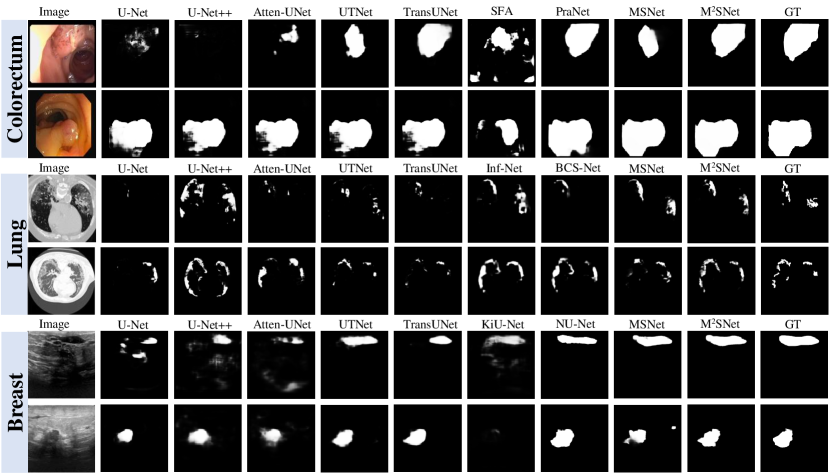
Figure 6: Visual comparison of different medicine-general and medicine-specific methods.

Table 7: Ablation experiments of the subtraction unit, inter-layer multi-scale aggregation and LossNet.

	ColonDB				ETIS
Methods	mDice $\uparrow$	mIoU $\uparrow$	$F_{\beta}^{w}$ $\uparrow$	$E_{\phi}^{max}$ $\uparrow$	mDice $\uparrow$	mIoU $\uparrow$	$F_{\beta}^{w}$ $\uparrow$	$E_{\phi}^{max}$ $\uparrow$
baseline ($SU_{1}^{i}$)	0.678	0.607	0.659	0.825	0.588	0.549	0.532	0.707
+ $SU_{2}^{i}$	0.731	0.652	0.703	0.861	0.642	0.579	0.586	0.745
+ $SU_{3}^{i}$	0.733	0.659	0.712	0.861	0.642	0.580	0.581	0.745
+ $SU_{4}^{i}$	0.750	0.676	0.729	0.872	0.643	0.580	0.585	0.757
+ $SU_{5}^{i}$	0.749	0.676	0.729	0.878	0.643	0.582	0.600	0.787
+ $\mathcal{L}_{f}$	0.755	0.678	0.737	0.883	0.719	0.664	0.678	0.830
$SU$ $\rightarrow$ $AU$	0.697	0.630	0.676	0.839	0.680	0.621	0.636	0.820

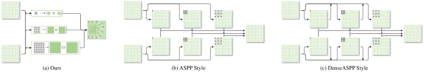
Figure 7: Illustration of different multi-scale modules applied in the subtraction unit.

Table 8: Ablation experiments of the intra-layer multi-scale subtraction design. Positive and negative gains are highlighted in red and blue, respectively.

	Efficiency		ETIS				CVC-300-TV				CVOID			BUSI
Methods	FLOPs $\downarrow$	Params $\downarrow$	mDice $\uparrow$	mIoU $\uparrow$	$F_{\beta}^{w}$ $\uparrow$	$E_{\phi}^{max}$ $\uparrow$	mDice $\uparrow$	mIoU $\uparrow$	$S_{\alpha}$ $\uparrow$	MAE$\downarrow$	DSC $\uparrow$	$S_{\alpha}$ $\uparrow$	MAE$\downarrow$	Jaccard $\uparrow$	Specificity $\uparrow$	Dice $\uparrow$
MSNet	9.0 G	27.7 M	0.719	0.664	0.678	0.830	0.837	0.755	0.895	0.014	0.779	0.846	0.007	70.57$\pm$3.38	98.29$\pm$0.44	78.18$\pm$3.75
M2SNet (ASPP)	13.8 G	29.2 M	0.711	0.644	0.671	0.838	0.827	0.752	0.890	0.014	0.809	0.855	0.006	60.23$\pm$1.94	98.14$\pm$0.42	68.52$\pm$1.82
$\Delta$ gains	- 53.3%	- 5.4%	-1.1%	- 3.0%	- 1.0%	- 1.0%	- 1.2%	- 0.4%	- 0.6%	0.0%	+ 3.9%	+ 1.1%	+ 14.3%	- 14.7%	- 0.2%	- 12.4%
M2SNet (DenseASPP)	17.5 G	29.6 M	0.709	0.645	0.668	0.833	0.869	0.798	0.916	0.010	0.798	0.853	0.006	63.11$\pm$4.63	98.42$\pm$0.59	71.71$\pm$4.33
$\Delta$ gains	- 94.4%	- 6.9%	-1.4%	- 2.9%	- 1.5%	- 0.4%	+ 3.8%	+ 5.7%	+ 2.3%	+ 28.6%	+ 2.4%	+ 0.8%	+ 14.3%	- 10.6%	+ 0.1%	- 8.3%
M2SNet (Ours)	9.0 G	27.7 M	0.749	0.678	0.712	0.872	0.876	0.805	0.918	0.010	0.795	0.855	0.006	71.52$\pm$1.19	98.35$\pm$0.20	79.21$\pm$1.38
$\Delta$ gains	0.0%	0.0%	+ 4.2%	+ 2.1%	+ 5.0%	+ 5.1%	+ 4.7%	+ 6.6%	+ 2.6%	+ 28.6%	+ 2.1%	+ 1.1%	+ 14.3%	+ 1.3%	+ 0.1%	+ 1.3%

4.4 Comparisons with State-of-the-art Methods

For a fair comparison, we compare not only with medicine-specific methods but also with representative medicine-general methods, including UNet [2], UNet++ [9], Attention U-Net [28], UTNet [7] and TransUNet [8]. Based on the open-source codes, we retrain these medicine-general methods on the same training sets as our models.
$\bullet$ In Tab. 1, among $30$ scores of all image polyp datasets, our multi-scale subtraction models (MSNet + M²SNet) achieve the best performance in terms of all six metrics. The M²SNet even outperforms the video-based polyp segmentation method PNS-Net [31] on the video polyp datasets, as shown in Tab. 2.
$\bullet$ Tab. 3 shows performance comparisons on the COVID-19 datasets. Compared to the second best method (Inf-Net [33]), M²SNet achieves an important improvement of $1.5\%$, $6.6\%$ and $14.3\%$ in terms of DSC, Precision and MAE, respectively.
$\bullet$ Tab. 4 shows performance comparisons with breast tumor segmentation methods. Following most methods [35, 36] in this field, we adopt the four-fold cross-validation strategy. M²SNet achieves the best performance in terms of the Jaccard, Precision and Dice metrics, which outperforms representative transformer-based methods, UTNet and TransUNet. Moreover, M²SNet has the smallest mean standard deviation ($0.97$) under the five metrics, which indicates its performance stability.
$\bullet$ In Tab. 5, we list the top $10$ OCT layer segmentation results in MICCAI2022 GOALS Challenge. More details please see the leaderboard. Based on the M²SNet, we won the second place (2/100) according to the weighted score of six results in three different layers. It is worth noting that our method ranks the top $1$ in four out of six metrics.
$\bullet$ As can be seen from Tab. 1 - Tab. 4, our M²SNet consistently surpasses other medicine-general methods in all medical segmentation sub-branches. In Tab. 6, we list the FLOPs and parameters of different medicine-general methods. It can be seen that our method has only 9GB in FLOPs, which has obvious advantages in terms of computational efficiency.
$\bullet$ Fig. 6 depicts a qualitative comparison with other methods. It can be seen that the results of M²SNet have greater advantages in terms of detection accuracy, completeness, and sharpness across different image modalities.

4.5 Ablation Study

We take the common FPN network as the baseline to analyze the contribution of each component.

4.5.1 Effectiveness of the subtraction unit, inter-layer multi-scale subtraction aggregation and LossNet

The results are shown in Tab 7. These defined feature subscripts are the same as those in Fig 2. First, we apply the basic subtraction unit (SU) to the baseline to get a series of $SU_{2}^{i}$ features to participate in the feature aggregation calculated by Equ. 1. The gap between the “ + $SU_{2}^{i}$ ” and the baseline demonstrates the effectiveness of the SU. It can be seen that the usage of SU has a significant improvement on the ColonDB dataset compared to the baseline, with the gain of 7.8%, 7.4%, 6.7% and 4.4% in terms of mDice, mIoU, $F_{\beta}^{w}$, and $E_{\phi}^{max}$, respectively. Next, we gradually add $SU_{3}^{i}$, $SU_{4}^{i}$ and $MS_{5}^{i}$ to achieve inter-layer multi-scale aggregation. The gap between the “ + $SU_{5}^{i}$ ” and the “ + $SU_{2}^{i}$ ” quantitatively demonstrates the effectiveness of inter-layer multi-scale subtraction strategy. Next, we evaluate the benefit of $\mathcal{L}_{f}$. Compared to the “ + $SU_{5}^{i}$ ” model, the “ + $\mathcal{L}_{f}$ ” achieves significant performance improvement on the ETIS dataset, with the gain of 11.8%, 14.1%, 13.0% and 5.5% in terms of mDice, mIoU, $F_{\beta}^{w}$, and $E_{\phi}^{max}$, respectively. Besides, we replace all subtraction units with the element-wise addition units (AU) and compare their performance. It can be seen that our subtraction units have significant advantage and no additional parameters are introduced.

4.5.2 Effectiveness of the intra-layer multi-scale subtraction design

Compared to the previous MSNet, the M²SNet replace all the original single-scale subtraction unit with the stronger multi-scale subtraction unit. As can be seen from Tab. 1 - Tab. 4, M²SNet shows significant improvement over MSNet on ten datasets of three tasks. To further show the advantages of our intra-layer multi-scale design, we apply other popular multi-scale modules (i.e., ASPP [16] and DenseASPP [17]) to the subtraction unit and these architectures are shown in Fig. 7. In Tab. 8, we thoroughly compare both the efficiency and accuracy of these three structures. It can be seen that “M²SNet (Ours)” has a significant performance gain in terms of fourteen metrics on four challenges datasets under different tasks. However, the other two models not only increase the computational burden by more than 50%, but also produce negative gains in multiple datasets. Therefore, the proposed intra-layer multi-scale subtraction design can be taken as a new baseline for future research in subtraction family.

To more intuitively show the differential information from different scales, we visualize all the features of the multi-scale in multi-scale subtraction module, as shown in Fig 8. We can see that the multi-scale in multi-scale subtraction module can clearly highlight the difference between high-level features and other level features and propagate its localization effect to the low-level ones. At the same level, the intra-layer multi-scale aggregation design can comprehensively capture both the subtle and regional difference features. Thus, both the global structural information and local boundary information is well depicted in the enhanced features of different levels.

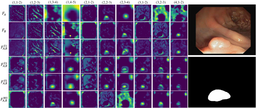
Figure 8: Visualization of the feature maps in the multi-scale in multi-scale subtraction module.

5 Discussion

Multi-scale Subtraction Unit: Different from previous addition and concatenation operations, using subtraction in multi-level structure make resulted features input to the decoder have much less redundancy among different levels and their level-specific properties are significantly enhanced. In this work, we further explore the potential of the subtraction unit in intra-layer multi-scale fusion. How to improve the accuracy while maintaining the same efficiency as the single-scale one is the key challenge. We provide the solution of using multi-scale convolution filters with fixed parameters. Compared to the single-scale design, multi-scale subtraction unit can enable the network to collect more complementary information both in pixel-pixel and neighbor-neighbor levels. The advantages of multi-scale subtraction unit in terms of efficiency and accuracy can be seen in Tab. 8. Multi-scale information extraction and feature aggregation are two general problems in the field of computer vision. Our multi-scale subtraction unit can solve both of them at once. We think this new paradigm can drive more researches on the subtraction operation in the future.
LossNet: LossNet is similar in form to perception loss [64] that has been applied in many tasks, such as style transfer and inpainting. While in those vision tasks, the perception-like loss is mainly used to speed the convergence of GAN and obtain high frequency information and ease checkerboard artifacts, but it does not bring obvious accuracy improvement. In our paper, the inputs are binary segmentation masks, LossNet can directly target the geometric features of the lesion and perform joint supervisions from the contour to the body, thereby improving the overall segmentation accuracy.

6 Conclusion

In this paper, we rethink previous addition-based or concatenation-based methods and present a simple yet general multi-scale in multi-scale subtraction network (M²SNet) for more efficient medical image segmentation. Based on the proposed intra-layer multi-scale subtraction unit, we pyramidally aggregate adjacent levels to extract lower-order and higher-order cross-level complementary information and combine with level-specific information to enhance multi-scale feature representation. Besides, we design a loss function based on a training-free network to supervise the prediction from different feature levels, which can optimize the segmentation on both structure and details during the backward phase. Experimental results on $11$ benchmark datasets towards $4$ medical segmentation tasks demonstrate that the proposed model outperforms various state-of-the-art methods.

References

- [1] T.-Y. Lin, P. Dollár, R. Girshick, K. He, B. Hariharan, and S. Belongie, “Feature pyramid networks for object detection,” in CVPR, 2017, pp. 2117–2125.
- [2] O. Ronneberger, P. Fischer, and T. Brox, “U-Net: Convolutional networks for biomedical image segmentation,” in MICCAI, 2015, pp. 234–241.
- [3] D. Jha, P. H. Smedsrud, M. A. Riegler, D. Johansen, T. De Lange, P. Halvorsen, and H. D. Johansen, “Resunet++: An advanced architecture for medical image segmentation,” in IEEE ISM, 2019, pp. 225–2255.
- [4] D.-P. Fan, G.-P. Ji, T. Zhou, G. Chen, H. Fu, J. Shen, and L. Shao, “Pranet: Parallel reverse attention network for polyp segmentation,” in MICCAI, 2020, pp. 263–273.
- [5] L. Zhang, J. Dai, H. Lu, Y. He, and G. Wang, “A bi-directional message passing model for salient object detection,” in CVPR, 2018, pp. 1741–1750.
- [6] X. Zhao, Y. Pang, L. Zhang, H. Lu, and L. Zhang, “Suppress and balance: A simple gated network for salient object detection,” in ECCV, 2020, pp. 35–51.
- [7] Y. Gao, M. Zhou, and D. N. Metaxas, “Utnet: a hybrid transformer architecture for medical image segmentation,” in MICCAI, 2021, pp. 61–71.
- [8] J. Chen, Y. Lu, Q. Yu, X. Luo, E. Adeli, Y. Wang, L. Lu, A. L. Yuille, and Y. Zhou, “Transunet: Transformers make strong encoders for medical image segmentation,” arXiv preprint arXiv:2102.04306, 2021.
- [9] Z. Zhou, M. M. R. Siddiquee, N. Tajbakhsh, and J. Liang, “Unet++: Redesigning skip connections to exploit multiscale features in image segmentation,” IEEE TMI, vol. 39, no. 6, pp. 1856–1867, 2019.
- [10] X. Qin, Z. Zhang, C. Huang, M. Dehghan, O. R. Zaiane, and M. Jagersand, “U2-net: Going deeper with nested u-structure for salient object detection,” Pattern Recognition, vol. 106, p. 107404, 2020.
- [11] Y. Pang, X. Zhao, L. Zhang, and H. Lu, “Multi-scale interactive network for salient object detection,” in CVPR, 2020, pp. 9413–9422.
- [12] X. Zhao, L. Zhang, Y. Pang, H. Lu, and L. Zhang, “A single stream network for robust and real-time rgb-d salient object detection,” in ECCV, 2020, pp. 646–662.
- [13] Z. Deng, X. Hu, L. Zhu, X. Xu, J. Qin, G. Han, and P.-A. Heng, “R3net: Recurrent residual refinement network for saliency detection,” in IJCAI, 2018, pp. 684–690.
- [14] W. Ji, J. Li, M. Zhang, Y. Piao, and H. Lu, “Accurate rgb-d salient object detection via collaborative learning,” in ECCV, 2020, pp. 52–69.
- [15] K. Fu, D.-P. Fan, G.-P. Ji, and Q. Zhao, “Jl-dcf: Joint learning and densely-cooperative fusion framework for rgb-d salient object detection,” in CVPR, 2020, pp. 3052–3062.
- [16] L.-C. Chen, G. Papandreou, I. Kokkinos, K. Murphy, and A. L. Yuille, “Deeplab: Semantic image segmentation with deep convolutional nets, atrous convolution, and fully connected crfs,” IEEE TPAMI, vol. 40, pp. 834–848, 2017.
- [17] M. Yang, K. Yu, C. Zhang, Z. Li, and K. Yang, “Denseaspp for semantic segmentation in street scenes,” in CVPR, 2018, pp. 3684–3692.
- [18] J. Zhang, D.-P. Fan, Y. Dai, S. Anwar, F. S. Saleh, T. Zhang, and N. Barnes, “Uc-net: Uncertainty inspired rgb-d saliency detection via conditional variational autoencoders,” in CVPR, 2020, pp. 8582–8591.
- [19] H. Mei, G.-P. Ji, Z. Wei, X. Yang, X. Wei, and D.-P. Fan, “Camouflaged object segmentation with distraction mining,” in CVPR, 2021, pp. 8772–8781.
- [20] L. Zhu, Z. Deng, X. Hu, C.-W. Fu, X. Xu, J. Qin, and P.-A. Heng, “Bidirectional feature pyramid network with recurrent attention residual modules for shadow detection,” in ECCV, 2018, pp. 121–136.
- [21] J. Kim and W. Kim, “Attentive feedback feature pyramid network for shadow detection,” IEEE SPL, vol. 27, pp. 1964–1968, 2020.
- [22] Y. Piao, W. Ji, J. Li, M. Zhang, and H. Lu, “Depth-induced multi-scale recurrent attention network for saliency detection,” in ICCV, 2019, pp. 7254–7263.
- [23] Y. Lv, J. Zhang, Y. Dai, A. Li, B. Liu, N. Barnes, and D.-P. Fan, “Simultaneously localize, segment and rank the camouflaged objects,” in CVPR, 2021, pp. 11 591–11 601.
- [24] J. Long, E. Shelhamer, and T. Darrell, “Fully convolutional networks for semantic segmentation,” in CVPR, 2015, pp. 3431–3440.
- [25] Z. Wang, E. P. Simoncelli, and A. C. Bovik, “Multiscale structural similarity for image quality assessment,” in The Thrity-Seventh Asilomar Conference on Signals, Systems & Computers, vol. 2, 2003, pp. 1398–1402.
- [26] Y. Pang, X. Zhao, T.-Z. Xiang, L. Zhang, and H. Lu, “Zoom in and out: A mixed-scale triplet network for camouflaged object detection,” in CVPR, 2022, pp. 2160–2170.
- [27] X. Zhao, L. Zhang, and H. Lu, “Automatic polyp segmentation via multi-scale subtraction network,” in MICCAI, 2021, pp. 120–130.
- [28] O. Oktay, J. Schlemper, L. L. Folgoc, M. Lee, M. Heinrich, K. Misawa, K. Mori, S. McDonagh, N. Y. Hammerla, B. Kainz et al., “Attention u-net: Learning where to look for the pancreas,” arXiv preprint arXiv:1804.03999, 2018.
- [29] A. Vaswani, N. Shazeer, N. Parmar, J. Uszkoreit, L. Jones, A. N. Gomez, L. Kaiser, and I. Polosukhin, “Attention is all you need,” in NeurIPS, 2017, p. 5998–6008.
- [30] Y. Fang, C. Chen, Y. Yuan, and K.-y. Tong, “Selective feature aggregation network with area-boundary constraints for polyp segmentation,” in MICCAI, 2019, pp. 302–310.
- [31] G.-P. Ji, Y.-C. Chou, D.-P. Fan, G. Chen, H. Fu, D. Jha, and L. Shao, “Progressively normalized self-attention network for video polyp segmentation,” in MICCAI, 2021, pp. 142–152.
- [32] N. Paluru, A. Dayal, H. B. Jenssen, T. Sakinis, L. R. Cenkeramaddi, J. Prakash, and P. K. Yalavarthy, “Anam-net: Anamorphic depth embedding-based lightweight cnn for segmentation of anomalies in covid-19 chest ct images,” IEEE TNNLS, vol. 32, no. 3, pp. 932–946, 2021.
- [33] D.-P. Fan, T. Zhou, G.-P. Ji, Y. Zhou, G. Chen, H. Fu, J. Shen, and L. Shao, “Inf-net: Automatic covid-19 lung infection segmentation from ct images,” IEEE TMI, vol. 39, no. 8, pp. 2626–2637, 2020.
- [34] R. Cong, H. Yang, Q. Jiang, W. Gao, H. Li, C. Wang, Y. Zhao, and S. Kwong, “Bcs-net: Boundary, context, and semantic for automatic covid-19 lung infection segmentation from ct images,” IEEE TIM, vol. 71, pp. 1–11, 2022.
- [35] M. Byra, P. Jarosik, A. Szubert, M. Galperin, H. Ojeda-Fournier, L. Olson, M. O’Boyle, C. Comstock, and M. Andre, “Breast mass segmentation in ultrasound with selective kernel u-net convolutional neural network,” BSPC, vol. 61, p. 102027, 2020.
- [36] G.-P. Chen, L. Li, Y. Dai, and J.-X. Zhang, “Nu-net: An unpretentious nested u-net for breast tumor segmentation,” arXiv preprint arXiv:2209.07193, 2022.
- [37] R. Zhang, G. Li, Z. Li, S. Cui, D. Qian, and Y. Yu, “Adaptive context selection for polyp segmentation,” in MICCAI, 2020, pp. 253–262.
- [38] Q. Hou, M.-M. Cheng, X. Hu, A. Borji, Z. Tu, and P. H. Torr, “Deeply supervised salient object detection with short connections,” in CVPR, 2017, pp. 3203–3212.
- [39] T.-Y. Lin, P. Goyal, R. Girshick, K. He, and P. Dollár, “Focal loss for dense object detection,” in ICCV, 2017, pp. 2980–2988.
- [40] F. Milletari, N. Navab, and S.-A. Ahmadi, “V-net: Fully convolutional neural networks for volumetric medical image segmentation,” in 2016 fourth international conference on 3D vision (3DV). IEEE, 2016, pp. 565–571.
- [41] S. S. M. Salehi, D. Erdogmus, and A. Gholipour, “Tversky loss function for image segmentation using 3d fully convolutional deep networks,” in International workshop on machine learning in medical imaging, 2017, pp. 379–387.
- [42] K. C. Wong, M. Moradi, H. Tang, and T. Syeda-Mahmood, “3d segmentation with exponential logarithmic loss for highly unbalanced object sizes,” in MICCAI, 2018, pp. 612–619.
- [43] S. A. Taghanaki, Y. Zheng, S. K. Zhou, B. Georgescu, P. Sharma, D. Xu, D. Comaniciu, and G. Hamarneh, “Combo loss: Handling input and output imbalance in multi-organ segmentation,” CMIG, vol. 75, pp. 24–33, 2019.
- [44] J. Wei, S. Wang, and Q. Huang, “F3net: Fusion, feedback and focus for salient object detection,” in AAAI, 2020, pp. 12 321–12 328.
- [45] X. Qin, Z. Zhang, C. Huang, C. Gao, M. Dehghan, and M. Jagersand, “Basnet: Boundary-aware salient object detection,” in CVPR, 2019, pp. 7479–7489.
- [46] N. Tajbakhsh, S. R. Gurudu, and J. Liang, “Automated polyp detection in colonoscopy videos using shape and context information,” IEEE TMI, vol. 35, no. 2, pp. 630–644, 2015.
- [47] J. Silva, A. Histace, O. Romain, X. Dray, and B. Granado, “Toward embedded detection of polyps in wce images for early diagnosis of colorectal cancer,” IJCARS, vol. 9, no. 2, pp. 283–293, 2014.
- [48] D. Jha, P. H. Smedsrud, M. A. Riegler, P. Halvorsen, T. de Lange, D. Johansen, and H. D. Johansen, “Kvasir-seg: A segmented polyp dataset,” in MMM, 2020, pp. 451–462.
- [49] D. Vázquez, J. Bernal, F. J. Sánchez, G. Fernández-Esparrach, A. M. López, A. Romero, M. Drozdzal, and A. Courville, “A benchmark for endoluminal scene segmentation of colonoscopy images,” JHE, vol. 2017, 2017.
- [50] J. Bernal, F. J. Sánchez, G. Fernández-Esparrach, D. Gil, C. Rodríguez, and F. Vilariño, “Wm-dova maps for accurate polyp highlighting in colonoscopy: Validation vs. saliency maps from physicians,” CMIG, vol. 43, pp. 99–111, 2015.
- [51] J. Bernal, J. Sánchez, and F. Vilarino, “Towards automatic polyp detection with a polyp appearance model,” Pattern Recognition, vol. 45, no. 9, pp. 3166–3182, 2012.
- [52] “Covid-19 ct segmentation dataset,” in https://medicalsegmentation.com/COVID19/, accessed April, 2020.
- [53] “Covid-19 ct lung and infection segmentation dataset,” in https://zenodo.org/record/3757476, accessed April 20, 2020.
- [54] S. Y. Shin, S. Lee, I. D. Yun, S. M. Kim, and K. M. Lee, “Joint weakly and semi-supervised deep learning for localization and classification of masses in breast ultrasound images,” IEEE TMI, vol. 38, no. 3, pp. 762–774, 2018.
- [55] W. Al-Dhabyani, M. Gomaa, H. Khaled, and A. Fahmy, “Dataset of breast ultrasound images,” Data in brief, vol. 28, p. 104863, 2020.
- [56] H. Fang, F. Li, H. Fu, J. Wu, X. Zhang, and Y. Xu, “Dataset and evaluation algorithm design for goals challenge,” arXiv preprint arXiv:2207.14447, 2022.
- [57] R. Margolin, L. Zelnik-Manor, and A. Tal, “How to evaluate foreground maps?” in CVPR, 2014, pp. 248–255.
- [58] D.-P. Fan, M.-M. Cheng, Y. Liu, T. Li, and A. Borji, “Structure-measure: A new way to evaluate foreground maps,” in ICCV, 2017, pp. 4548–4557.
- [59] D.-P. Fan, C. Gong, Y. Cao, B. Ren, M.-M. Cheng, and A. Borji, “Enhanced-alignment Measure for Binary Foreground Map Evaluation,” in IJCAI, 2018.
- [60] F. Shan, Y. Gao, J. Wang, W. Shi, N. Shi, M. Han, Z. Xue, D. Shen, and Y. Shi, “Lung infection quantification of covid-19 in ct images with deep learning,” arXiv preprint arXiv:2003.04655, 2020.
- [61] G. Chen, L. Li, Y. Dai, J. Zhang, and M. H. Yap, “Aau-net: An adaptive attention u-net for breast lesions segmentation in ultrasound images,” IEEE TMI, 2022.
- [62] Z. Chen, Q. Xu, R. Cong, and Q. Huang, “Global context-aware progressive aggregation network for salient object detection,” in AAAI, 2020, pp. 10 599–10 606.
- [63] T. Zhou, H. Fu, G. Chen, Y. Zhou, D.-P. Fan, and L. Shao, “Specificity-preserving rgb-d saliency detection,” in ICCV, 2021, pp. 4681–4691.
- [64] J. Johnson, A. Alahi, and L. Fei-Fei, “Perceptual losses for real-time style transfer and super-resolution,” in ECCV, 2016, pp. 694–711.