Explicit Visual Prompting for Low-Level Structure Segmentations

Abstract

We consider the generic problem of detecting low-level structures in images, which includes segmenting the manipulated parts, identifying out-of-focus pixels, separating shadow regions, and detecting concealed objects. Whereas each such topic has been typically addressed with a domain-specific solution, we show that a unified approach performs well across all of them. We take inspiration from the widely-used pre-training and then prompt tuning protocols in NLP and propose a new visual prompting model, named Explicit Visual Prompting (EVP). Different from the previous visual prompting which is typically a dataset-level implicit embedding, our key insight is to enforce the tunable parameters focusing on the explicit visual content from each individual image, i.e., the features from frozen patch embeddings and the input’s high-frequency components. The proposed EVP significantly outperforms other parameter-efficient tuning protocols under the same amount of tunable parameters (5.7$\%$ extra trainable parameters of each task). EVP also achieves state-of-the-art performances on diverse low-level structure segmentation tasks compared to task-specific solutions. Our code is available at: https://github.com/NiFangBaAGe/Explicit-Visual-Prompt.

1 Introduction

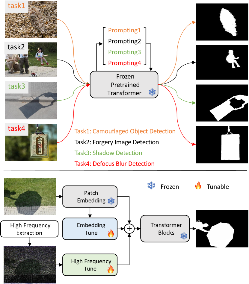
Figure 1: We propose a unified method for four low-level structure segmentation tasks: camouflaged object, forgery, shadow and defocus blur detection (Top). Our approach relies on a pre-trained frozen transformer backbone that leverages explicit extracted features, e.g., the frozen embedded features and high-frequency components, to prompt knowledge.

Advances in image editing and manipulation algorithms have made it easy to create photo-realistic but fake pictures [31, 63, 39]. Detecting such manipulated regions becomes an important problem due to its potential negative impact related to surveillance and crime [31]. Low-level structures are known to be beneficial to tampered region detection, i.e., resizing and copy-pasting will destroy the JPEG compression levels between the temper region and the host image [50, 28, 62], the noise level of the tempered region and the background is also different [87, 76]. Interesting, to segment the blurred pixels [67], shadowed regions [59], and concealed objects [15], low-level clues also play important roles. These detection tasks are shown to be beneficial to numerous computer vision tasks, including auto-refocus [1], image retargeting [37], object tracking [55], etc.

Although all these tasks belong to low-level structure segmentation, they are typically addressed by domain-specific solutions with carefully designed network architectures [87, 8, 90]. Moreover, the lack of large-scale datasets is often considered a major factor, which limits the performances [31].

In this work, we propose a solution to address the four tasks in a unified fashion. We take inspiration from recent advances of prompting [33, 4, 2], which is a concept that initially emerged in natural language processing (NLP) [3]. The basic idea is to efficiently adapt a frozen large foundation model to many downstream tasks with the minimum extra trainable parameters. As the foundation model has already been trained on a large-scale dataset, prompting often leads to better model generalization on the downstream tasks [3], especially in the case of the limited annotated data. Prompting also significantly saves the storage of models since it only needs to save a shared basic model and task-aware promptings.

Our main insight is to tune the task-specific knowledge only from the features of each individual image itself because the pre-trained base model contains sufficient knowledge for semantic understanding. This is also inspired by the effectiveness of hand-crafted image features, such as SIFT [29], JPEG noise [50], resampling artifacts [62] in these tasks [46, 50, 29, 28, 62, 87].

Based on this observation, we propose explicit visual prompting (EVP), where the tuning performance can be hugely improved via the re-modulation of image features. Specifically, we consider two kinds of features for our task. The first is the features from the frozen patch embedding, which is critical since we need to shift the distribution of the original model. Another is high-frequency components of the input image since the pre-trained visual recognition model is learned to be invariant to these features via data augmentation. As shown in Figure 1, we take a model pre-trained on a large-scale dataset and freeze its parameters. Then, to adapt to each task, we tune the embedded features and learn an extra embedding for high-frequency components of each individual image.

In terms of experiments, we validate our approach on nine datasets of four tasks: forgery detection, shadow detection, defocus blur detection as well as camouflaged object detection. Our simple and unified network achieves very competitive performance with the whole model fine-tuning and outperforms task-specific solutions without modification.

In summary, our main contributions are as follows:

• We design a unified approach that produces state-of-the-art performances for a number of tasks, including forgery detection, defocus blur detection, shadow detection, and camouflaged object detection.

• We propose explicit visual prompting (EVP), which takes the features from the frozen patch embedding and the input’s high-frequency components as prompting. It is demonstrated to be effective across different tasks and outperforms other parameter-efficient tuning methods.

• Our method greatly simplifies the low-level structure segmentation models as well as achieves comparable performance with well-designed SOTA methods.

2 Related Work

Visual Prompting Tuning.

Prompting is initially proposed in NLP [3, 45]. [3] demonstrates strong generalization to downstream transfer learning tasks even in the few-shot or zero-shot settings with manually chosen prompts in GPT-3. Recently, prompting [65, 33] has been adapted to vision tasks. [65] proposes memory tokens which is a set of learnable embedding vectors for each transformer layer. VPT [33] proposes similar ideas and investigates the generality and feasibility of visual prompting via extensive experiments spanning multiple kinds of recognition tasks across multiple domains and backbone architectures. Unlike VPT, whose main focus is on recognition tasks, our work aims at exploring optimal visual content for low-level structure segmentation.

Forgery Detection.

The goal of forgery detection is to detect pixels that are manually manipulated, such as pixels that are removed, replaced, or edited. Early approaches [53, 52, 20, 7] detect region splicing through inconsistencies in local noise levels, based on the fact that images of different origins might contain different noise characteristics introduced by the sensors or post-processing steps. Other clues are found to be helpful, such as SIFT [29], JPEG compression artifacts [50] and re-sampling artifacts [16, 62]. Recently, approaches have moved towards end-to-end deep learning methods for solving specific forensics tasks using labeled training data [32, 75, 86, 64, 26]. Salloum et al. [64] learn to detect splicing by training a fully convolutional network on labeled training data. [75, 86, 76, 26, 47] propose improved architectures. Islam et al. [32] incorporate Generative Adversarial Network (GAN) to detect copy-move forgeries. Huh et al. [31] propose to take photographic metadata as a free and plentiful supervisory signal for learning self-consistency and apply the trained model to detect splices. Recently, TransForensic [22] leverages vision transformers [13] to tackle the problem. High-frequency components still served as useful prior in this field. RGB-N [87] designs an additional noise stream. ObjectFormer [74] extracts high-frequency features as complementary signals to visual content. But unlike ObjectFormer, our main focus is to leverage high-frequency components as a prompting design to efficiently and effectively adapt to different low-level segmentation tasks.

Defocus Blur Detection.

Given an image, defocus blur detection aims at separating in-focus and out-of-focus regions, which could be potentially useful for auto-refocus [1], salient object detection [34] and image retargeting [37]. Traditional approaches mainly focus on designing hand-crafted features based on gradient [67, 78, 21] or edge [38, 68]. In the deep era, most methods delve into CNN architectures [60, 82, 70, 83]. [60] proposes the first CNN-based method using both hand-crafted and deep features. BTBNet [82] develops a fully convolutional network to integrate low-level clues and high-level semantic information. DeFusionNet [70] recurrently fuses and refines multi-scale deep features for defocus blur detection. CENet [83] learns multiple smaller defocus blur detectors and ensembles them to enhance diversity. [8] further employs the depth information as additional supervision and proposes a joint learning framework inspired by knowledge distillation. [79] explores deep ensemble networks for defocus blur detection. [80] proposes to learn generator to generate mask in an adversarial manner.

Shadow Detection.

Shadows occur frequently in natural scenes, and have hints for scene geometry [58], light conditions [58] and camera location  [36] and lead to challenging cases in many vision tasks including image segmentation [14] and object tracking [6, 56]. Early attempts explore illumination  [19, 18] and hand-crafted features [30, 41, 88]. In the deep era, some methods mainly focus on the design of CNN architectures [89, 9] or involving the attention modules (e.g., the direction-aware attention [27], distraction-aware module [84]). Recent works [42, 90] utilize the lighting as additional prior, for example, ADNet [42] generates the adversarial training samples for better detection and FDRNet [90] arguments the training samples by additionally adjusted brightness. MTMT [5] leverages the mean teacher model to explore unlabeled data for semi-supervised shadow detection.

Camouflaged Object Detection.

Detecting camouflaged objects is a challenging task as foreground objects are often with visual similar patterns to the background. Early works distinguish the foreground and background through low-level clues such as texture [66, 17], brightness [61], and color [25]. Recently, deep learning-based methods [15, 54, 44, 51, 35] show their strong ability in detecting complex camouflage objects. Le et al. [43] propose the first end-to-end network for camouflaged object detection, which is composed of a classification branch and a segmentation branch. Fan et al. [15] develops a search-identification network and the largest camouflaged object detection dataset. PFNet [54] is a bio-inspired framework that mimics the process of positioning and identification in predation. FBNet [35] suggests disentangling frequency modeling and enhancing the important frequency component.

3 Method

In this section, we propose Explicit Visual Prompting (EVP) for adapting recent Vision Transformers (SegFormer [77] as the example) pre-trained on ImageNet [10] to low-level structure segmentations. EVP keeps the backbone frozen and only contains a small number of tunable parameters to learn task-specific knowledge from the features of frozen image embeddings and high-frequency components. Below, we first present SegFormer[77] and the extraction of high-frequency components in Section 3.1, then the architecture design in Section 3.2.

3.1 Preliminaries

SegFormer [77].

SegFormer is a hierarchical transformer-based structure with a much simpler decoder for semantic segmentation. Similar to traditional CNN backbone [23], SegFormer captures multi-stale features via several stages. Differently, each stage is built via the feature embedding layers and vision transformer blocks [71, 13]. As for the decoder, it leverages the multi-scale features from the encoder and MLP layers for decoding to the specific classes. Notice that, the proposed prompt strategy is not limited to SegFormer and can be easily adapted to other network structures, e.g., ViT [13] and Swin [49].

Figure 2: The procedure to generate high-frequency components.

High-frequency Components (HFC).

As shown in Figure 2, for an image $I$ of dimension $H\times W$, we can decompose it into low-frequency components $I_{l}$ (LFC) and high-frequency components $I_{h}$ (HFC), i.e. $I=\{I_{l},I_{h}\}$. Denoting $\mathtt{fft}$ and $\mathtt{ifft}$ as the Fast Fourier Transform and its inverse respectively, we use $z$ to represent the frequency component of $I$. Therefore we have $z=\mathtt{fft}(I)$ and $I=\mathtt{ifft}(z)$. We shift low frequency coefficients to the center $(\frac{H}{2},\frac{W}{2})$. To obtain HFC, a binary mask $\mathbf{M}_{h}\in\{0,1\}^{H\times W}$ is generated and applied on $z$ depending on a mask ratio $\tau$:

$$\mathbf{M}^{i,j}_{h}(\tau)=\begin{cases}0,&\frac{4|(i-\frac{H}{2})(j-\frac{W}{2})|}{HW}\leq\tau\\ 1,&\text{otherwise}\end{cases}$$ (1)

$\tau$ indicates the surface ratio of the masked regions. HFC can be computed:

$$I_{hfc}=\mathtt{ifft}(z\mathbf{M}_{h}(\tau))$$ (2)

Similarly, a binary mask $\mathbf{M}_{l}\in\{0,1\}^{H\times W}$ can be properly defined to compute LFC:

$$\mathbf{M}^{i,j}_{l}(\tau)=\begin{cases}0,&\frac{HW-4|(i-\frac{H}{2})(j-\frac{W}{2})|}{HW}\leq\tau\\ 1,&\text{otherwise}\end{cases}$$ (3)

and LFC can be calculated as:

$$I_{lfc}=\mathtt{ifft}(z\mathbf{M}_{l}(\tau))$$ (4)

Note that for RGB images, we compute the above process on every channel of pixels independently.

Figure 3: The architecture of the proposed explicit visual prompting. We use the Embedding Tune and the HFC Tune to tune the extracted features. The Adaptor is designed to merge these features.

3.2 Explicit Visual Prompting

In this section, we present the proposed Explicit Visual Prompting (EVP). Our key insight is to learn explicit prompts from image embeddings and high-frequency components. We learn the former to shift the distribution from the pre-train dataset to the target dataset. And the main motivation to learn the latter is that the pre-trained model is learned to be invariant to these features through data augmentation. Note that this is different from VPT [33], which learns implicit prompts. Our approach is illustrated in Figure 3, which is composed of three basic modules: patch embedding tune, high-frequency components tune as well as Adaptor.

Patch embedding tune.

This module aims at tuning pre-trained patch embedding. In pre-trained SegFormer [77], a patch $I^{p}$ is projected to a $C_{seg}$-dimension feature. We freeze this projection and add a tunable linear layer $\mathtt{L_{pe}}$ to project the original embedding into a $c$-dimension feature $F_{pe}\in\mathbb{R}^{c}$.

$$F_{pe}=\mathtt{L_{pe}}(I^{p})\text{, with }c=\frac{C_{seg}}{r}$$ (5)

where we introduce the scale factor $r$ to control the tunable parameters.

High-frequency components tune.

For the high frequency components $I_{hfc}$, we learn an overlapped patch embedding similar to SegFormer [77]. Formally, $I_{hfc}$ is divided into small patches with the same patch size as SegFormer [77]. Denoting patch $I^{p}_{hfc}\in\mathbb{R}^{C}$ and $C=h\times w\times 3$, we learn a linear layer $\mathtt{L_{hfc}}$ to project the patch into a $c$-dimension feature $F_{hfc}\in\mathbb{R}^{c}$.

$$F_{hfc}=\mathtt{L_{hfc}}(I^{p}_{hfc})$$ (6)

Adaptor.

The goal of Adaptor is to efficiently and effectively perform adaptation in all the layers by considering features from the image embeddings and high-frequency components. For the $i$-th Adaptor, we take $F_{pe}$ and $F_{hfc}$ as input and obtain the prompting $P^{i}$:

$$P^{i} =\mathtt{MLP_{up}({GELU(\mathtt{MLP^{i}_{tune}}(F_{pe}+F_{hfc}))})}$$ (7)

where $\mathtt{GELU}$ is GELU [24] activation. $\mathtt{MLP^{i}_{tune}}$ is a linear layer for producing different prompts in each Adaptor. $\mathtt{MLP_{up}}$ is an up-projection layer shared across all the Adaptors for matching the dimension of transformer features. $P^{i}$ is the output prompting that attaches to each transformer layer.

4 Experiment

Task	Dataset Name	# Train	# Test
Forgery Detection	CAISA [12]	5,123	921
	IMD20 [57]	-	2,010
Shadow Detection	ISTD [73]	1,330	540
	SBU [72]	4,089	638
Defocus Blur Detection	CUHK [67]	604	100
	DUT [81]	-	500
Camouflaged Object Detection	COD10K [15]	3,040	2,026
	CAMO [43]	1,000	250
	CHAMELEON  [69]	-	76

Table 1: Summary of datasets considered in this work. We show the number of images in training (# Train) and testing set (# Test) for different datasets.

Method	DUT [81]		CUHK [67]
	$F_{\beta}\uparrow$	MAE$\downarrow$	$F_{\beta}\uparrow$	MAE$\downarrow$
DeFusionNet [70]	.823	.118	.818	.117
BTBNet [82]	.827	.138	.889	.082
CENet [83]	.817	.135	.906	.059
DAD [80]	.794	.153	.884	.079
EFENet [79]	.854	.094	.914	.053
Ours	.890	.068	.928	.045

Table 2: Comparison with state-of-the-art approaches on defocus blur detection.

Method	ISTD [73]	SBU [72]
	BER$\downarrow$	BER$\downarrow$
BDRAR [89]	2.69	3.89
DSC [27]	3.42	5.59
DSD [84]	2.17	3.45
MTMT [5]	1.72	3.15
FDRNet [90]	1.55	3.04
Ours	1.35	4.31

Table 3: Comparison with state-of-the-art approaches on shadow detection.

Method	IMD20 [57]		CAISA [12]
	F1$\uparrow$	AUC$\uparrow$	F1$\uparrow$	AUC$\uparrow$
ManTra [76]	-	.748	-	.817
SPAN [26]	-	.750	.382	.838
PSCCNet [48]	-	.806	.554	.875
TransForensics [22]	-	.848	.627	.837
ObjectFormer [74]	-	.821	.579	.882
Ours	.443	.807	.636	.862

Table 4: Comparison with state-of-the-art approaches on forgery detection.

Method	CHAMELEON [69]				CAMO [43]				COD10K [15]
	$S_{\alpha}\uparrow$	$E_{\phi}$ $\uparrow$	$F_{\beta}^{w}$ $\uparrow$	MAE $\downarrow$	$S_{\alpha}\uparrow$	$E_{\phi}$ $\uparrow$	$F_{\beta}^{w}$ $\uparrow$	MAE $\downarrow$	$S_{\alpha}\uparrow$	$E_{\phi}$ $\uparrow$	$F_{\beta}^{w}$ $\uparrow$	MAE $\downarrow$
SINet [15]	.869	.891	.740	.044	.751	.771	.606	.100	.771	.806	.551	.051
RankNet [51]	.846	.913	.767	.045	.712	.791	.583	.104	.767	.861	.611	.045
JCOD [44]	.870	.924	-	.039	.792	.839	-	.082	.800	.872	-	.041
PFNet [54]	.882	.942	.810	.033	.782	.852	.695	.085	.800	.868	.660	.040
FBNet [35]	.888	.939	.828	.032	.783	.839	.702	.081	.809	.889	.684	.035
Ours	.871	.917	.795	.036	.846	.895	.777	.059	.843	.907	.742	.029

Table 5: Comparison with state-of-the-art approaches on camouflaged object detection.

Method	Trainable	Defocus Blur		Shadow	Forgery		Camouflaged
	Param.	CUHK [67]		ISTD [73]	CASIA [12]		CAMO [43]
	(M)	$F_{\beta}\uparrow$	MAE $\downarrow$	BER $\downarrow$	$F_{1}\uparrow$	AUC $\uparrow$	$S_{\alpha}\uparrow$	$E_{\phi}$ $\uparrow$	$F_{\beta}^{w}$ $\uparrow$	MAE $\downarrow$
Full-tuning	64.00	.935	.039	2.42	.465	.754	.837	.887	.778	.060
Only Decoder	3.15	.891	.080	4.36	.396	.722	.783	.827	.671	.088
VPT-Deep [33]	3.27	.913	.058	1.73	.588	.847	.833	.884	.751	.068
AdaptFormer [4]	3.21	.912	.057	1.85	.602	.855	.830	.877	.750	.068
Ours (r=16)	3.22	.924	.051	1.67	.602	.857	.838	.888	.761	.065
Ours (r=4)	3.70	.928	.045	1.35	.636	.862	.846	.895	.777	.059

Table 6: Comparison with state-of-the-art efficient tuning approaches. We conduct evaluations on four datasets for four different tasks. The efficient tuning method which achieves better performance than full-tuning is marked as orange. The best performance among all methods is shown as blod.

4.1 Datasets

We evaluate our model on a variety of datasets for four tasks: forgery detection, shadow detection, defocus blur detection, and camouflaged object detection. A summary of the basic information of these datasets is illustrated in Table 1.

Forgery Detection.

CASIA [12] is a large dataset for forgery detection, which is composed of 5,123 training and 921 testing spliced and copy-moved images. IMD20 [57] is a real-life forgery image dataset that consists of 2, 010 samples for testing. We follow the protocol of previous works [48, 22, 74] to conduct the training and evaluation at the resolution of $256\times 256$. We use pixel-level Area Under the Receiver Operating Characteristic Curve (AUC) and $F_{1}$ score to evaluate the performance.

Shadow Detection.

SBU [72] is the largest annotated shadow dataset which contains 4,089 training and 638 testing samples, respectively. ISTD [73] contains triple samples for shadow detection and removal, we only use the shadowed image and shadow mask to train our method. Following [5, 89, 90], we train and test both datasets with the size of $400\times 400$. As for the evaluation metrics, We report the balance error rate (BER).

Defocus Blur Detection.

Following previous work [81, 8], we train the defocus blur detection model in the CUHK dataset [67], which contains a total of 704 partial defocus samples. We train the network on the 604 images split from the CUHK dataset and test in DUT [81] and the rest of the CUHK dataset. The images are resized into $320\times 320$, following [8]. We report performances with commonly used metrics: F-measure ($F_{\beta}$) and mean absolute error (MAE).

Camouflaged Object Detection.

COD10K [15] is the largest dataset for camouflaged object detection, which contains 3,040 training and 2,026 testing samples. CHAMELEON [69] includes 76 images collected from the Internet for testing. CAMO [43] provides diverse images with naturally camouflaged objects and artificially camouflaged objects. Following [15, 54], we train on the combined dataset and test on the three datasets. We employ commonly used metrics: S-measure ($S_{m}$), mean E-measure ($E_{\phi}$), weighted F-measure ($F_{\beta}^{w}$), and MAE for evaluation.

4.2 Implementation Details

All the experiments are performed on a single NVIDIA Titan V GPU with 12G memory. AdamW [40] optimizer is used for all the experiments. The initial learning rate is set to $2e^{-4}$ for defocus blur detection and camouflaged object detection, and $5e^{-4}$ for others. Cosine decay is applied to the learning rate. The models are trained for 20 epochs for the SBU [72] dataset and camouflaged combined dataset [15, 69], and 50 epochs for others. Random horizontal flipping is applied during training for data augmentation. The mini-batch is equal to 4. Binary cross-entropy (BCE) loss is used for defocus blur detection and forgery detection, balanced BCE loss is used for shadow detection, and BCE loss and IOU loss are used for camouflaged object detection. All the experiments are conducted with SegFormer-B4 [77] pre-trained on the ImageNet-1k [11] dataset.

Figure 4: Comparisons with other task-specific methods. We show the results of: SINet [15] and PFNet [54] on CAMO [43] dataset for camouflaged object detection (Top-left), ManTra [76] and SPAN [26] on CAISA [12] dataset for forgery detection (Top-right), MTMT [5] and FDRNet [90] on ISTD [73] dataset for shadow detection (Bottom-left), CENet [83] and EFENet [79] on CUHK [67] dataset for defocus blur detection (Bottom-right).

Method	Trainable	Defocus Blur		Shadow	Forgery		Camouflaged
	Param.	CUHK [67]		ISTD [73]	CASIA [12]		CAMO [43]
	(M)	$F_{\beta}\uparrow$	MAE $\downarrow$	BER $\downarrow$	$F_{1}\uparrow$	AUC $\uparrow$	$S_{\alpha}\uparrow$	$E_{\phi}$ $\uparrow$	$F_{\beta}^{w}$ $\uparrow$	MAE $\downarrow$
Decoder (No prompting)	3.15	.891	.080	4.36	.396	.722	.783	.827	.671	.088
Ours w/o $F_{pe}$	3.61	.924	.049	1.68	.540	.833	.840	.887	.759	.065
Ours w/o $F_{hfc}$	3.58	.926	.046	1.61	.619	.846	.844	.893	.773	.063
Ours w/ Shared $\mathtt{MLP^{i}_{tune}}$	3.49	.928	.048	1.77	.619	.860	.837	.889	.763	.064
Ours w/ Unshared $\mathtt{MLP_{up}}$	4.54	.927	.045	1.33	.647	.875	.844	.893	.774	.060
Ours	3.70	.928	.045	1.35	.636	.862	.846	.895	.777	.059

Table 7: Ablation on the architecture designs described in Figure 3. We conduct evaluations on four datasets for four different tasks. The proposed prompting strategy (Decoder + $F_{hfc}$ + $F_{pe}$ + Adaptor) performs more effectively.

Tuning	Trainable	Defocus Blur		Shadow	Forgery		Camouflaged
Stage	Param.	CUHK [67]		ISTD [73]	CASIA [12]		CAMO [43]
	(M)	$F_{\beta}\uparrow$	MAE $\downarrow$	BER $\downarrow$	$F_{1}\uparrow$	AUC $\uparrow$	$S_{\alpha}\uparrow$	$E_{\phi}$ $\uparrow$	$F_{\beta}^{w}$ $\uparrow$	MAE $\downarrow$
Stage1	3.16	.895	.072	3.64	.408	.725	.793	.834	.681	.088
Stage1,2	3.18	.917	.058	2.45	.457	.765	.806	.853	.706	.081
Stage1,2,3	3.43	.927	.047	1.46	.627	.858	.841	.888	.768	.062
Stage1,2,3,4	3.70	.928	.045	1.35	.636	.862	.846	.895	.777	.059

Table 8: Ablation on the tuning stages in SegFormer. We conduct evaluations on four datasets for four different tasks. The performance of EVP becomes better as the tuning stages increase.

$r$	Trainable	Defocus Blur		Shadow	Forgery		Camouflaged
	Param.	CUHK [67]		ISTD [73]	CASIA [12]		CAMO [43]
	(M)	$F_{\beta}\uparrow$	MAE $\downarrow$	BER $\downarrow$	$F_{1}\uparrow$	AUC $\uparrow$	$S_{\alpha}\uparrow$	$E_{\phi}$ $\uparrow$	$F_{\beta}^{w}$ $\uparrow$	MAE $\downarrow$
64	3.17	.910	.055	2.09	.547	.830	.829	.875	.743	.070
32	3.18	.919	.054	1.84	.574	.844	.832	.877	.749	.067
16	3.22	.924	.051	1.67	.602	.857	.838	.888	.761	.065
8	3.34	.923	.049	1.46	.619	.856	.841	.890	.767	.062
4	3.70	.928	.045	1.35	.636	.862	.846	.895	.777	.059
2	4.95	.929	.042	1.31	.642	.859	.842	.896	.776	.059
1	9.56	.931	.040	1.48	.621	.847	.843	.894	.778	.059

Table 9: Ablation on the parameter scale factor $r$. We conduct evaluations on four datasets for four different tasks. EVP gets the balance between the number of tunable parameters and performances when $r=4$.

Method	Trainable	Defocus Blur		Shadow	Forgery		Camouflaged
	Param.	CUHK [67]		ISTD [73]	CASIA [12]		CAMO [43]
	(M)	$F_{\beta}\uparrow$	MAE $\downarrow$	BER $\downarrow$	$F_{1}\uparrow$	AUC $\uparrow$	$S_{\alpha}\uparrow$	$E_{\phi}$ $\uparrow$	$F_{\beta}^{w}$ $\uparrow$	MAE $\downarrow$
Full-tuning	98.98	.862	.077	4.39	.290	.650	.593	.677	.382	.157
Only Decoder	13.00	.836	.097	4.77	.318	.662	.615	.659	.385	.162
VPT [33]	13.09	.843	.092	4.56	.315	.666	.615	.660	.387	.161
AdaptFormer [4]	13.08	.845	.092	4.60	.319	.662	.614	.662	.387	.161
EVP	13.06	.850	087	4.36	.324	.675	.622	.674	.402	.156

Table 10: Comparison with other tuning methods with SETR [85] on four different tasks. We conduct an evaluation on four datasets for four different tasks. The best performance is shown as bold. The prompt-tuning method which achieves better performance than full-tuning is marked as orange.

4.3 Main Results

Comparison with the task-specific methods.

EVP performs well when compared with task-specific methods. We report the comparison of our methods and other task-specific methods in Table 5, Table 5, Table 5, and Table 5. Thanks to our stronger backbone and prompting strategy, EVP achieves the best performance in 5 datasets across 4 different tasks. However, compared with other well-designed domain-specific methods, EVP only introduces a small number of tunable parameters with the frozen backbone and obtains non-trivial performance. We also show some visual comparisons with other methods for each task individually in Figure 4. We can see the proposed method predicts more accurate masks compared to other approaches.

Comparison with the efficient tuning methods.

We evaluate our method with full finetuning and only tuning the decoder, which are the widely-used strategies for down-streaming task adaption. And similar methods from image classification, i.e., VPT [33] and AdaptFormer [4]. The number of prompt tokens is set to 10 for VPT and the middle dimension of AdaptMLP is set to 2 for a fair comparison in terms of the tunable parameters. It can be seen from Table 6 that when only tuning the decoder, the performance drops largely. Compared with similar methods, introducing extra learnable tokens [33] or MLPs in Transformer block [4] also benefits the performance. We introduce a hyper-parameter ($r$) which is used to control the number of parameters of the Adaptor as described in equation 5. We first compare EVP ($r$=16) with similar parameters as other methods. From the table, our method achieves much better performance. We also report EVP ($r$=4), with more parameters, the performance can be further improved and outperforms full-tuning on 3 of 4 datasets.

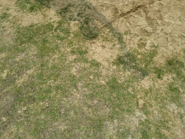
(a)

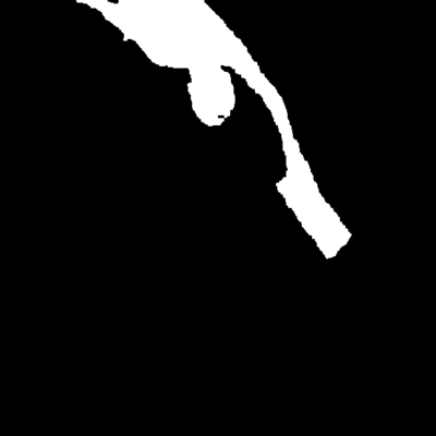
(b)

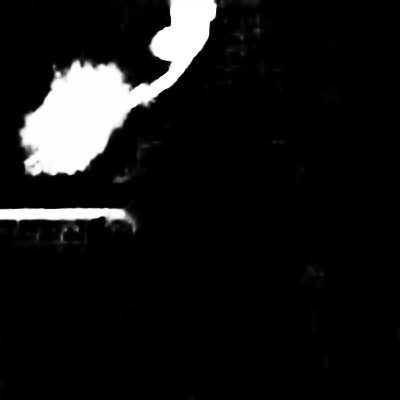
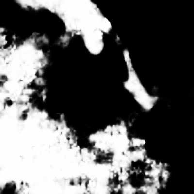
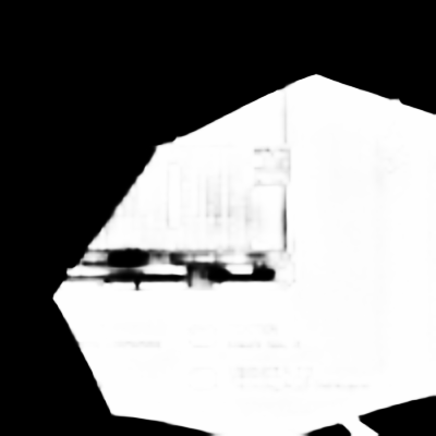
(c)

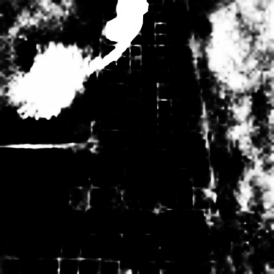
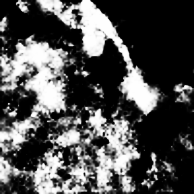
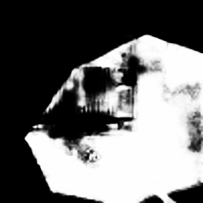
(d)

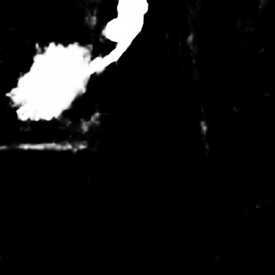
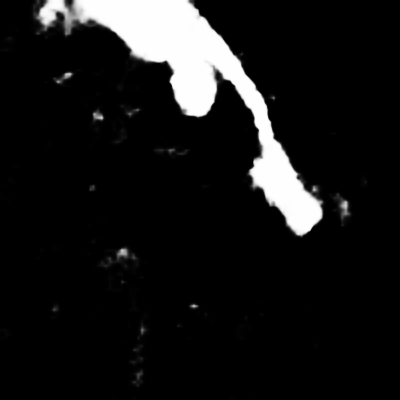
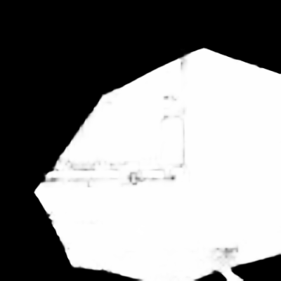
(e)

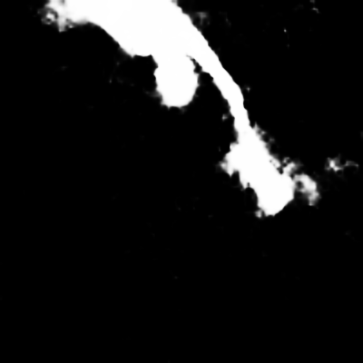
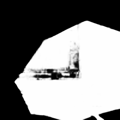
(f)

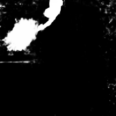
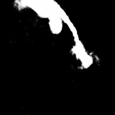
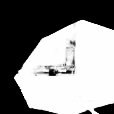
(g)

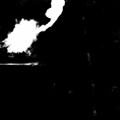
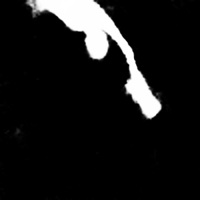
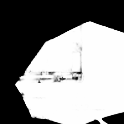
(h)

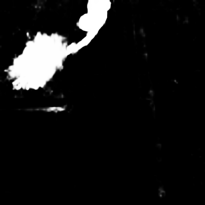
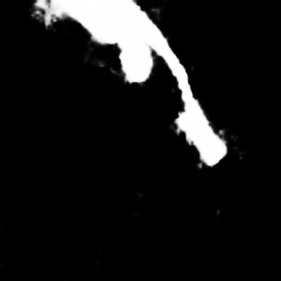
(i)

Figure 5: Quantitative comparison using full-tuning and different prompting designs on ISTD [73] dataset for shadow detection. From the left to right is: (a) Input, (b) GT, (c) Full-tuning, (d) Decoder (No prompting), (e) Ours w/o $F_{pe}$, (f) Ours w/o $F_{hfc}$, (g) Ours w/ Shared $\mathtt{MLP^{i}_{tune}}$, (h) Ours w/ Unshared $\mathtt{MLP_{up}}$, (i) Ours Full.

4.4 Ablation Study

We conduct the ablation to show the effectiveness of each component. The experiments are performed with the scaling factor $r=4$ except specified.

Architecture Design.

To verify the effectiveness of the proposed visual prompting architecture, we modify it into different variants. As shown in Table 7 and Figure 5, sharing $\mathtt{MLP^{i}_{tune}}$ in different Adaptors only saves a small number of parameters (0.55M v.s. 0.34M) but leads to a significant performance drop. It cannot obtain consistent performance improvement when using different $\mathtt{MLP_{up}}$ in different Adaptors, moreover introducing a large number of parameters (0.55M v.s. 1.39M). On the other hand, the performance will drop when we remove $F_{pe}$ or $F_{hfc}$, which means that they are both effective visual prompts.

Tuning Stage.

We try to answer the question: which stage contributes mostly to prompting tuning? Thus, we show the variants of our tuning method by changing the tunable stages in the SegFormer backbone. SegFormer contains 4 stages for multi-scale feature extraction. We mark the Stage_x where the tunable prompting is added in Stage $x$. Table 8 shows that better performance can be obtained via the tunable stages increasing. Besides, the maximum improvement occurs in Stage_1,2 to Stage_1,2,3. Note that the number of transformer blocks of each stage in SegFormer-B4 is 3, 8, 27, and 3, respectively. Thus, the effect of EVP is positively correlated to the number of the prompted transformer blocks.

Scale Factor $r$ (equation 5).

We introduce $r$ in Sec 3.2 of the main paper to control the number of learnable parameters. A larger $r$ will use fewer parameters for tuning. As shown in Table 9, the performance improves on several tasks when $r$ decreases from 64 to 4; when $r$ continues to decrease to 2 or 1, it can not gain better performance consistently even if the model becomes larger. It indicates that $r=4$ is a reasonable choice to make a trade-off between the performance and model size.

EVP in Plain ViT.

We experiment on SETR [85] to confirm the generalizability of EVP. SETR employs plain ViT as the backbone and a progressive upsampling ConvNet as the decoder, while SegFormer has a hierarchical backbone with 4 stages. Therefore, the only distinction between the experiments using SegFormer is that all modifications are limited to the single stage in plain ViT. The experiments are conducted with ViT-Base [13] pretrained on the ImageNet-21k [11] dataset. The number of prompt tokens is set to 10 for VPT, the middle dimension of AdaptMLP is set to 4 for AdaptFormer, and $r$ is set to 32 for our EVP. As shown in Table 10, EVP also outperforms other tuning methods when using plain ViT as the backbone.

5 Conclusion

In this paper, we present explicit visual prompting to unify the solutions of low-level structure segmentations. We mainly focus on two kinds of features: the frozen features from patch embedding and the high-frequency components from the original image. Equipped with our method, we find that a frozen vision transformer backbone from the ImageNet with limited tunable parameters can achieve similar performance as the full-tuned network structures, also the state-of-the-art performance compared with the other task-specific methods. For future works, we will extend our approach to other related problems and hope it can promote further exploration of visual prompting.

Acknowledgments.

This work was supported in part by the University of Macau under Grant MYRG2022-00190-FST and in part by the Science and Technology Development Fund, Macau SAR, under Grants: 0034/2019/AMJ, 0087/2020/A2, and 0049/2021/A.

Appendix A Implementation Details

We give more implementation details in the main paper of the ”comparison with the task-specific methods” and ”comparison with the efficient tuning methods”.

Basic Setting.

Our method contains a backbone for feature extraction and a decoder for segmentation prediction. We initialize the weight of the backbone via ImageNet classification pre-training, and the weight of the decoder is randomly initialized. Below, we give the details of each variant.

Full-tuning.

We follow the basic setting above, and then, fine-tune all the parameters of the encoder and decoder.

Only Decoder.

We follow the basic setting above, and then, fine-tune the parameters in the decoder only.

VPT [33].

We first initialize the model following the basic setting. Then, we concatenate the prompt embeddings in each transformer block of the backbone only. Notice that, their prompt embeddings are implicitly shared across the whole dataset. We follow their original paper and optimize the parameters in the prompt embeddings and the decoder.

AdaptFormer [4].

We first initialize the model following the basic setting above. Then, the AdaptMLP is added to each transformer block of the backbone for feature adaptation. We fine-tune the parameters in the decoder and the newly introduced AdaptMLP.

EVP (Ours).

We also initialize the weight following the basic setting. Then, we add the explicit prompting as described in the main paper of Figure 3.

Metric.

AUC calculates the area of the ROC curve. ROC curve is a function of true positive rate ($\frac{tp}{tp+fn}$) in terms of false positive rate ($\frac{fp}{fp+tn}$), where $tp$, $tn$, $fp$, $fn$ represent the number of pixels which are classified as true positive, true negative, false positive, and false negative, respectively. $F_{1}$ score is defined as $F_{1}=\frac{2\times precision\times recall}{precision+recall}$, where $precision=\frac{tp}{tp+fp}$ and $recall=\frac{tp}{tp+fn}$. The balance error rate (BER) $=\left(1-\frac{1}{2}\left(\frac{tp}{tp+fn}+\frac{tn}{tn+fp}\right)\right)\times 100$. F-measure is calculated as $F_{\beta}=\frac{\left(1+\beta^{2}\right)\times precision\times recall}{\beta^{2}\times precision+recall}$, where $\beta^{2}=0.3$. MAE computes pixel-wise average distance. Weighted F-measure ($F_{\beta}^{w}$) weighting the quantities TP, TN, FP, and FN according to the errors at their location and their neighborhood information: $F_{\beta}^{w}=\frac{\left(1+\beta^{2}\right)\times precision^{w}\times recall^{w}}{\beta^{2}\times precision^{w}+recall^{w}}$. E-measure ($E_{\phi}$) jointly considers image statistics and local pixel matching: $E_{\phi}=\frac{1}{W\times H}\sum_{i=1}^{W}\sum_{j=1}^{H}\phi_{S}(i,j)$, where $\phi_{S}$ is the alignment matrix depending on the similarity of the prediction and ground truth.

Training Data.

Note that most forgery detection methods (ManTraNet [76], SPAN [26], PSCCNet [48], and ObjectFormer [74] in Table 5) and one shadow detection method (MTMT [5] in Table 5) use extra training data to get better performance. We only use the training data from the standard datasets and obtain SOTA performance.

Appendix B More Results

We provide more experimental results in addition to the main paper.

B.1 High-Frequency Prompting

Our method gets the knowledge from the explicit content of the image itself, hence we also discuss other similar explicit clues of images as the prompts. Specifically, we choose the common-used Gaussian filter, the noise-filter [20], the all-zero image, and the original image as experiments. From Table B11, we find the Gaussian filter shows a better performance in defocus blur since it is also a kind of blur. Also, the noise filter [20] from forgery detection also boosts the performance. Interestingly, we find that simply replacing the original image with an all-zero image also boosts the performance, since it can also be considered as a kind of implicitly learned embeddings across the full dataset as in VPT [33]. Differently, the high-frequency components of the image achieve consistent performance improvement to other methods on these several benchmarks.

B.2 HFC v.s. LFC

We conduct the ablation study on choosing of high-frequency features or the low-frequency features in Table B12. From the table, using the low-frequency components as the prompting just show some trivial improvement on these datasets. Differently, the high-frequency components are more general solutions and show a much better performance in shadow detection, forgery detection, and camouflaged detection. Similar to the Gaussian filter as we discussed above, the LFC is also a kind of blur, which makes the advantage of LFC in the defocus blur detection.

B.3 Mask Ratio $\tau$

We further evaluate the hyper-parameter mask ratio $\tau$ introduced in Section 3.1. From Table B12, when we mask out 25% of the central pixels in the spectrum, it achieves consistently better performance in all the tasks. We also find that the performance may drop when the increasing of mask ratio (all 0 images), especially in shadow detection, forgery detection, and camouflaged object detection.

Method	Defocus Blur		Shadow	Forgery		Camouflaged
	CUHK [67]		ISTD [73]	CASIA [12]		CAMO [43]
	$F_{\beta}\uparrow$	MAE $\downarrow$	BER $\downarrow$	$F_{1}\uparrow$	AUC $\uparrow$	$S_{\alpha}\uparrow$	$E_{\phi}$ $\uparrow$
Gaussian Blur	.928	.046	1.52	.631	.860	.842	.893
Noise Filter	.923	.046	1.47	.637	.866	.843	.894
All 0 Image	.922	.047	1.45	.630	.862	.844	.895
Original	.922	.047	1.59	.630	.860	.840	.891
HFC	.928	.045	1.35	.636	.862	.846	.895

Table B11: Ablation on the explicit visual prompting with other relatives. We compare with the widely-used image filter as prompting to verify the effectiveness of the proposed HFC.

Method	Mask	Defocus Blur		Shadow	Forgery		Camouflaged
	Ratio	CUHK [67]		ISTD [73]	CASIA [12]		CAMO [43]
	$\tau$ (%)	$F_{\beta}\uparrow$	MAE $\downarrow$	BER $\downarrow$	$F_{1}\uparrow$	AUC $\uparrow$	$S_{\alpha}\uparrow$	$E_{\phi}$ $\uparrow$
Low Frequency Components (LFC) with FFT
LFC*	0	.922	.047	1.45	.630	.862	.844	.895
LFC	10	.927	.046	1.58	.631	.862	.845	.895
LFC	25	.924	.047	1.49	.630	.860	.842	.891
LFC	50	.923	.048	1.48	.630	.860	.841	.893
LFC	75	.924	048	1.56	.627	.859	.840	.894
LFC	90	.925	.046	1.47	.626	.859	.841	.894
LFC**	100	.922	.047	1.59	.630	.860	.840	.891
High Frequency Components (HFC) with FFT
HFC	10	.926	.046	1.60	.631	.854	.843	.894
HFC	25	.928	.045	1.35	.636	.862	.846	.895
HFC	50	.925	.047	1.51	.631	.862	.843	.894
HFC	75	.923	.048	1.52	.629	.858	.842	.892
HFC	90	.924	.047	1.49	.630	.861	.842	.893

Table B12: Ablation on HFC, LFC, and mask ratio $\tau$. Leveraging FFT to extract high-frequency components consistently outperforms LFC. *LFC ($\tau$=0) equals to a full zero image for prompting. **LFC ($\tau$=100) means we learn an embedding from the original input image directly.

Appendix C Additional Visual Results

We give more visual results of EVP and other task-specific methods on the four tasks in Figure C6, C7, C8, and C9 as supplementary to the visual results in the main paper.

(a) Input

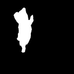
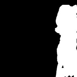
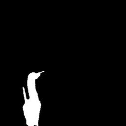
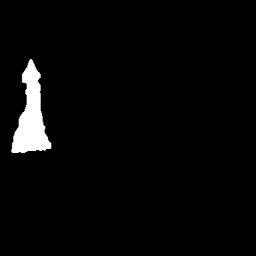
(b) GT

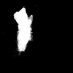
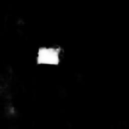
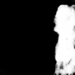
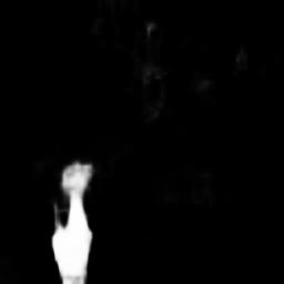
(c) Ours

(d) ManTraNet

(e) SPAN

Figure C6: More results on CAISA [12] dataset for forgery detection. We compare to ManTraNet [76] and SPAN [26].

(a) Input

(b) GT

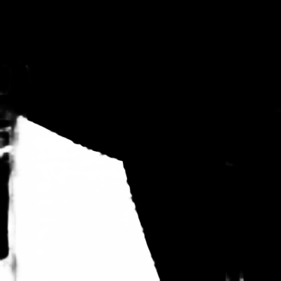
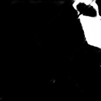
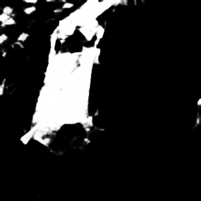
(c) Ours

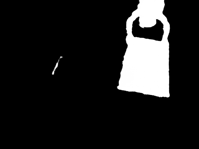
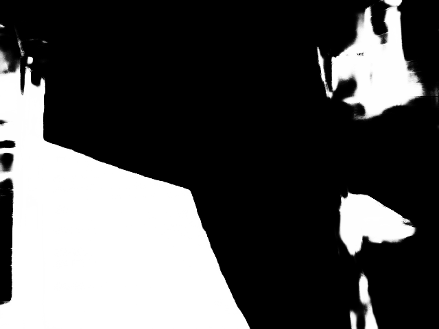
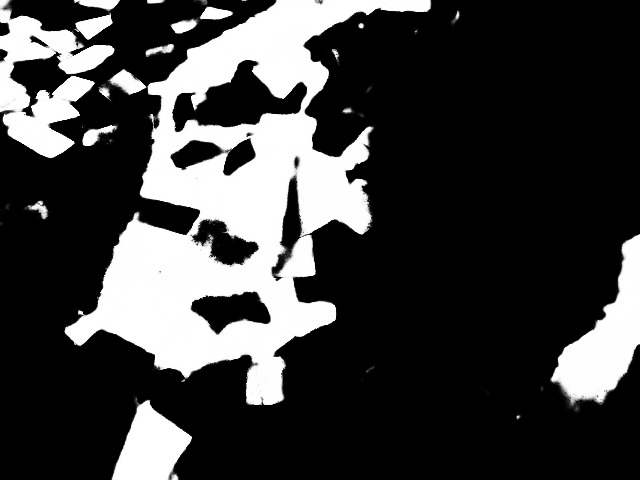
(d) DSD

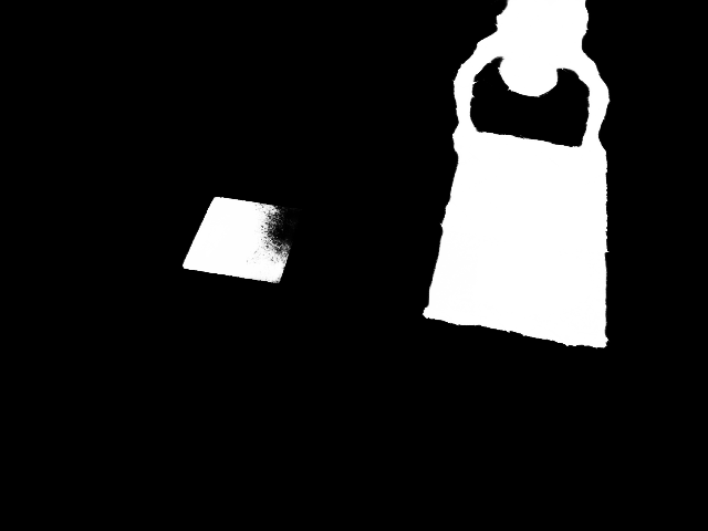
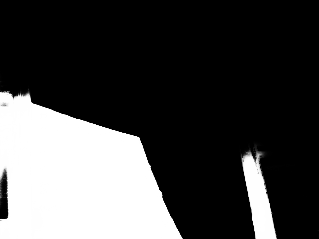
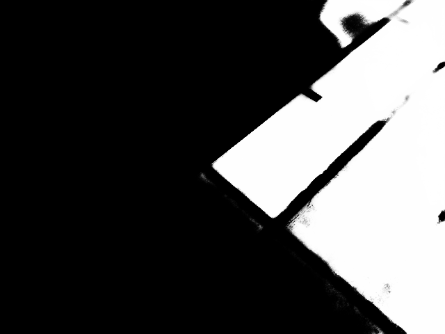
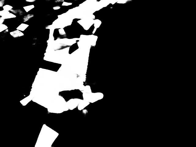
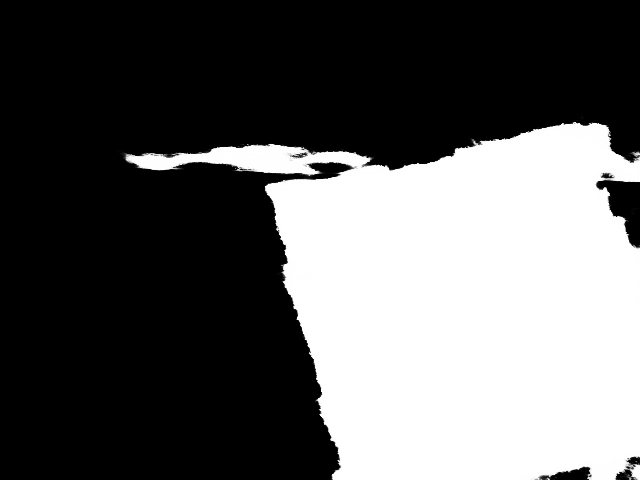
(e) MTMT

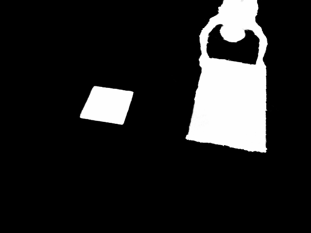
(f) FDRNet

Figure C7: More results on ISTD [73] dataset for shadow detection. We compare to DSD [80], MTMT [5], FDRNet [90].

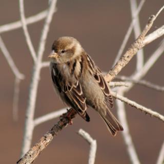
(a) Input

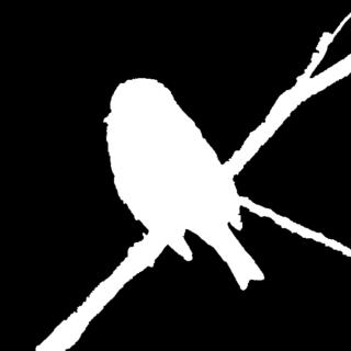
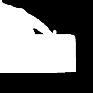
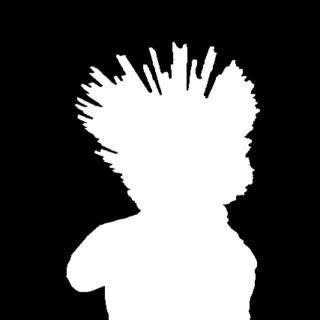
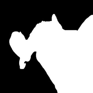
(b) GT

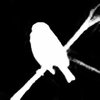
(c) Ours

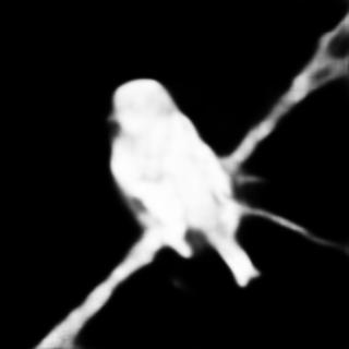
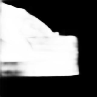
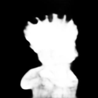
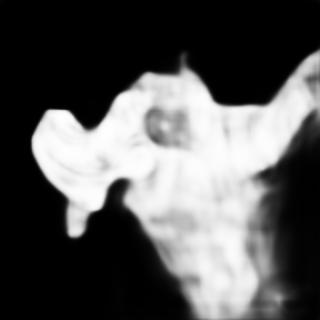
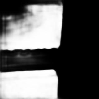
(d) BTBNet

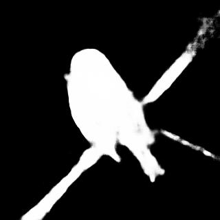
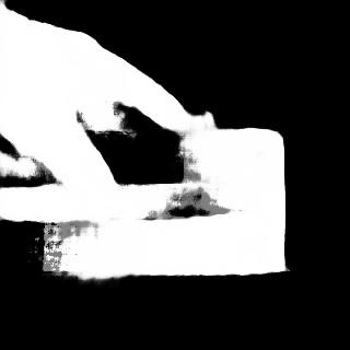
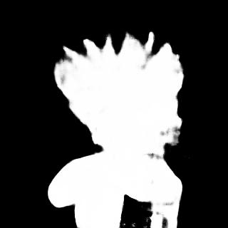
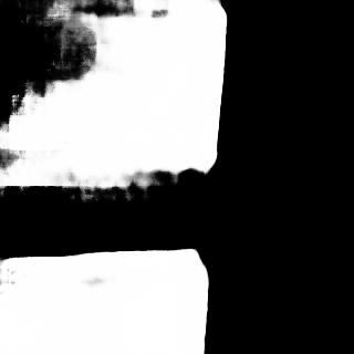
(e) CENet

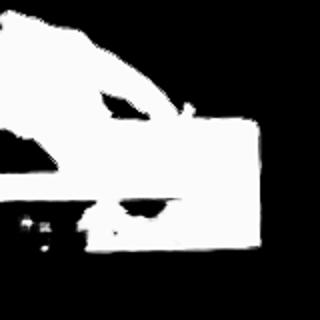
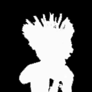
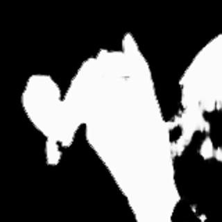
(f) EFENet

Figure C8: More results on CUHK [67] dataset for defocus blur detection.We compare to BTBNet [82], CENet [83] and EFENet [79].

(a) Input

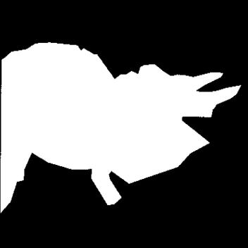
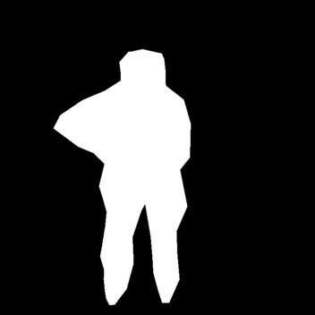
(b) GT

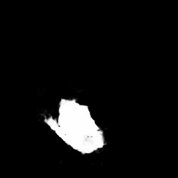
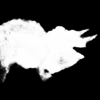
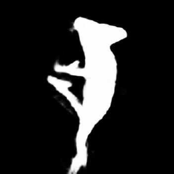
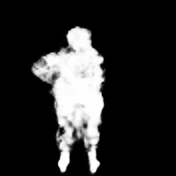
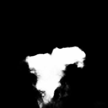
(c) Ours

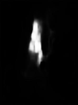
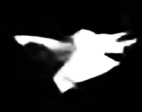
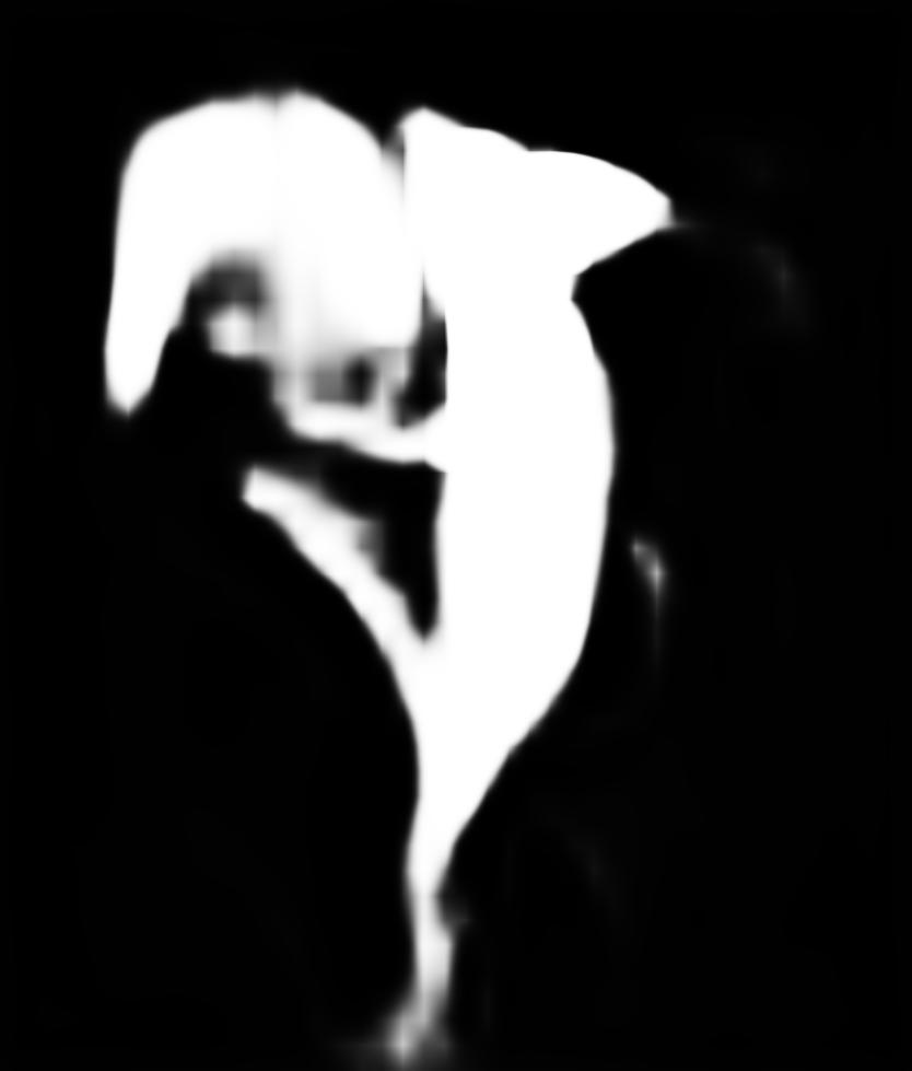
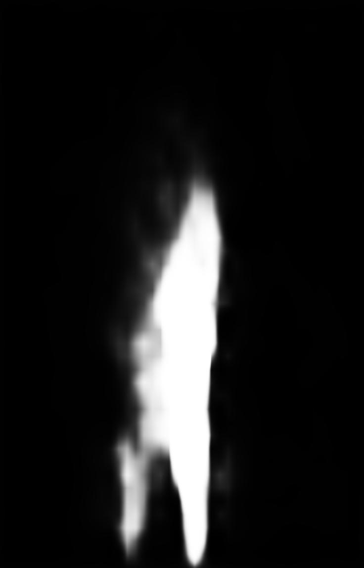
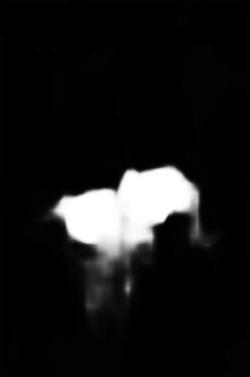
(d) SINet

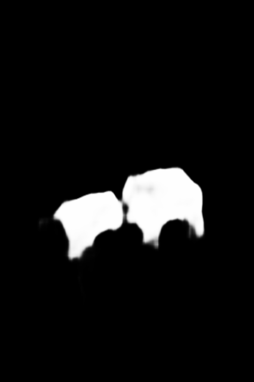
(e) PFNet

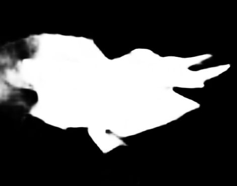
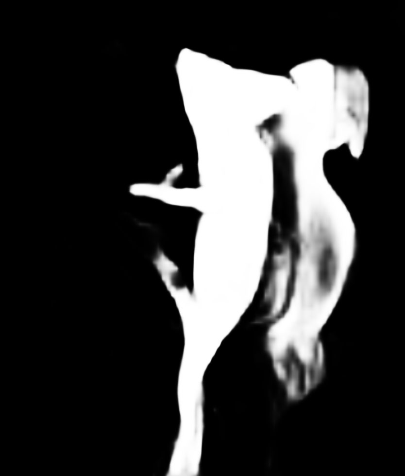
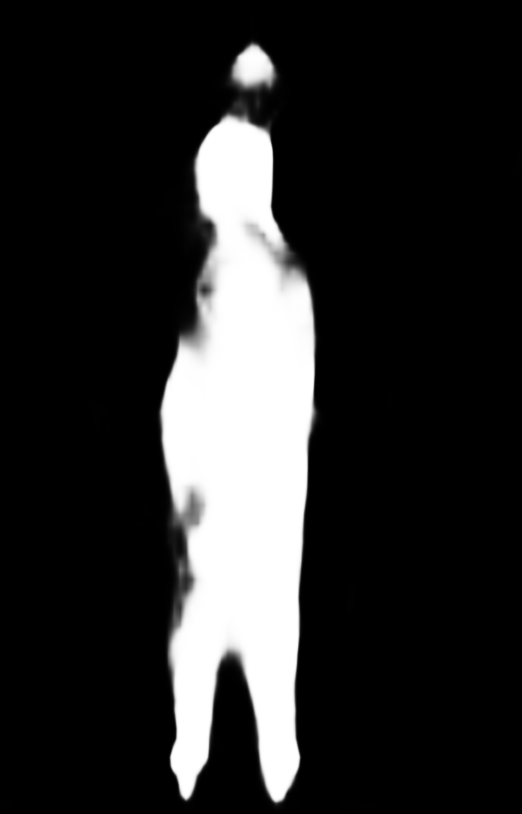
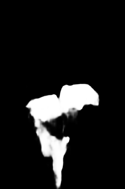
(f) JCOD

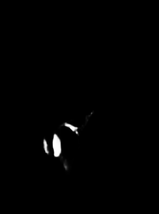
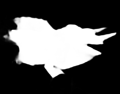
(g) RankNet

Figure C9: More results on CAMO [43] dataset for camouflaged object detection. We compare to SINet [15], PFNEt [54], JCOD [44] and RankNet [51].

References

- [1] Soonmin Bae and Frédo Durand. Defocus magnification. In Computer Graphics Forum, 2007.
- [2] Amir Bar, Yossi Gandelsman, Trevor Darrell, Amir Globerson, and Alexei A Efros. Visual prompting via image inpainting. In Advances in Neural Information Processing Systems (NeurIPS), 2022.
- [3] Tom Brown, Benjamin Mann, Nick Ryder, Melanie Subbiah, Jared D Kaplan, Prafulla Dhariwal, Arvind Neelakantan, Pranav Shyam, Girish Sastry, Amanda Askell, et al. Language models are few-shot learners. In Advances in Neural Information Processing Systems (NeurIPS), 2020.
- [4] Shoufa Chen, Chongjian Ge, Zhan Tong, Jiangliu Wang, Yibing Song, Jue Wang, and Ping Luo. Adaptformer: Adapting vision transformers for scalable visual recognition. In Advances in Neural Information Processing Systems (NeurIPS), 2022.
- [5] Zhihao Chen, Lei Zhu, Liang Wan, Song Wang, Wei Feng, and Pheng-Ann Heng. A multi-task mean teacher for semi-supervised shadow detection. In Proceedings of the Conference on Computer Vision and Pattern Recognition (CVPR), 2020.
- [6] Rita Cucchiara, Costantino Grana, Massimo Piccardi, and Andrea Prati. Detecting moving objects, ghosts, and shadows in video streams. Transactions on Pattern Analysis and Machine Intelligence (TPAMI), 2003.
- [7] Xiaodong Cun and Chi-Man Pun. Image splicing localization via semi-global network and fully connected conditional random fields. In Proceedings of the European Conference on Computer Vision Workshop (ECCVW), 2018.
- [8] Xiaodong Cun and Chi-Man Pun. Defocus blur detection via depth distillation. In Proceedings of the European Conference on Computer Vision (ECCV), 2020.
- [9] Xiaodong Cun, Chi-Man Pun, and Cheng Shi. Towards ghost-free shadow removal via dual hierarchical aggregation network and shadow matting gan. In Proceedings of the AAAI Conference on Artificial Intelligence (AAAI), 2020.
- [10] Jia Deng, Wei Dong, Richard Socher, Li-Jia Li, Kai Li, and Li Fei-Fei. Imagenet: A large-scale hierarchical image database. In Proceedings of the Conference on Computer Vision and Pattern Recognition (CVPR), 2009.
- [11] Jia Deng, Wei Dong, Richard Socher, Li-Jia Li, Kai Li, and Li Fei-Fei. Imagenet: A large-scale hierarchical image database. In Proceedings of the Conference on Computer Vision and Pattern Recognition (CVPR), 2009.
- [12] Jing Dong, Wei Wang, and Tieniu Tan. Casia image tampering detection evaluation database. In China Summit and International Conference on Signal and Information Processing, 2013.
- [13] Alexey Dosovitskiy, Lucas Beyer, Alexander Kolesnikov, Dirk Weissenborn, Xiaohua Zhai, Thomas Unterthiner, Mostafa Dehghani, Matthias Minderer, Georg Heigold, Sylvain Gelly, et al. An image is worth 16x16 words: Transformers for image recognition at scale. In ICLR, 2021.
- [14] Aleksandrs Ecins, Cornelia Fermüller, and Yiannis Aloimonos. Shadow free segmentation in still images using local density measure. In International Conference on Computational Photography (ICCP), 2014.
- [15] Deng-Ping Fan, Ge-Peng Ji, Guolei Sun, Ming-Ming Cheng, Jianbing Shen, and Ling Shao. Camouflaged object detection. In Proceedings of the IEEE/CVF conference on computer vision and pattern recognition, pages 2777–2787, 2020.
- [16] Xiaoying Feng, Ingemar J Cox, and Gwenael Doerr. Normalized energy density-based forensic detection of resampled images. Transactions on Multimedia, 2012.
- [17] Xue Feng, Cui Guoying, and Song Wei. Camouflage texture evaluation using saliency map. In Proceedings of the Fifth International Conference on Internet Multimedia Computing and Service, pages 93–96, 2013.
- [18] Graham D Finlayson, Mark S Drew, and Cheng Lu. Entropy minimization for shadow removal. 2009.
- [19] Graham D Finlayson, Steven D Hordley, Cheng Lu, and Mark S Drew. On the removal of shadows from images. IEEE transactions on pattern analysis and machine intelligence, 28(1):59–68, 2005.
- [20] Jessica Fridrich and Jan Kodovsky. Rich models for steganalysis of digital images. Transactions on information Forensics and Security, 2012.
- [21] S Alireza Golestaneh and Lina J Karam. Spatially-varying blur detection based on multiscale fused and sorted transform coefficients of gradient magnitudes. In Proceedings of the Conference on Computer Vision and Pattern Recognition (CVPR), 2017.
- [22] Jing Hao, Zhixin Zhang, Shicai Yang, Di Xie, and Shiliang Pu. Transforensics: image forgery localization with dense self-attention. In Proceedings of the IEEE/CVF International Conference on Computer Vision, pages 15055–15064, 2021.
- [23] Kaiming He, Xiangyu Zhang, Shaoqing Ren, and Jian Sun. Deep residual learning for image recognition. In CVPR, 2016.
- [24] Dan Hendrycks and Kevin Gimpel. Gaussian error linear units (gelus). arXiv, 2016.
- [25] Jianqin Yin Yanbin Han Wendi Hou and Jinping Li. Detection of the mobile object with camouflage color under dynamic background based on optical flow. Procedia Engineering, 15:2201–2205, 2011.
- [26] Xuefeng Hu, Zhihan Zhang, Zhenye Jiang, Syomantak Chaudhuri, Zhenheng Yang, and Ram Nevatia. Span: Spatial pyramid attention network for image manipulation localization. In Proceedings of the European Conference on Computer Vision (ECCV), 2020.
- [27] Xiaowei Hu, Lei Zhu, Chi-Wing Fu, Jing Qin, and Pheng-Ann Heng. Direction-aware spatial context features for shadow detection. In Proceedings of the Conference on Computer Vision and Pattern Recognition (CVPR), 2018.
- [28] Fangjun Huang, Jiwu Huang, and Yun Qing Shi. Detecting double jpeg compression with the same quantization matrix. Transactions on Information Forensics and Security, 2010.
- [29] Hailing Huang, Weiqiang Guo, and Yu Zhang. Detection of copy-move forgery in digital images using sift algorithm. In Pacific-Asia Workshop on Computational Intelligence and Industrial Application, 2008.
- [30] Xiang Huang, Gang Hua, Jack Tumblin, and Lance Williams. What characterizes a shadow boundary under the sun and sky? In 2011 international conference on computer vision, pages 898–905. IEEE, 2011.
- [31] Minyoung Huh, Andrew Liu, Andrew Owens, and Alexei A Efros. Fighting fake news: Image splice detection via learned self-consistency. In Proceedings of the European Conference on Computer Vision (ECCV), 2018.
- [32] Ashraful Islam, Chengjiang Long, Arslan Basharat, and Anthony Hoogs. Doa-gan: Dual-order attentive generative adversarial network for image copy-move forgery detection and localization. In Proceedings of the Conference on Computer Vision and Pattern Recognition (CVPR), 2020.
- [33] Menglin Jia, Luming Tang, Bor-Chun Chen, Claire Cardie, Serge Belongie, Bharath Hariharan, and Ser-Nam Lim. Visual prompt tuning. arXiv preprint arXiv:2203.12119, 2022.
- [34] Peng Jiang, Haibin Ling, Jingyi Yu, and Jingliang Peng. Salient region detection by ufo: Uniqueness, focusness and objectness. In Proceedings of the International Conference on Computer Vision (ICCV), 2013.
- [35] LIN Jiaying, TAN Xin, XU Ke, MA Lizhuang, and WH Rynson. Frequency-aware camouflaged object detection. ACM Transactions on Multimedia Computing, Communications and Applications, 2022.
- [36] Imran N Junejo and Hassan Foroosh. Estimating geo-temporal location of stationary cameras using shadow trajectories. In Proceedings of the European Conference on Computer Vision (ECCV), 2008.
- [37] Ali Karaali and Claudio Rosito Jung. Image retargeting based on spatially varying defocus blur map. In International Conference on Image Processing (ICIP), 2016.
- [38] Ali Karaali and Claudio Rosito Jung. Edge-based defocus blur estimation with adaptive scale selection. Transactions on Image Processing (TIP), 2017.
- [39] Bahjat Kawar, Shiran Zada, Oran Lang, Omer Tov, Huiwen Chang, Tali Dekel, Inbar Mosseri, and Michal Irani. Imagic: Text-based real image editing with diffusion models. arXiv, 2022.
- [40] Diederik P Kingma and Jimmy Ba. Adam: A method for stochastic optimization. arXiv preprint arXiv:1412.6980, 2014.
- [41] Jean-François Lalonde, Alexei A Efros, and Srinivasa G Narasimhan. Detecting ground shadows in outdoor consumer photographs. In European conference on computer vision, pages 322–335. Springer, 2010.
- [42] Hieu Le, Tomas F Yago Vicente, Vu Nguyen, Minh Hoai, and Dimitris Samaras. A+ d net: Training a shadow detector with adversarial shadow attenuation. In Proceedings of the European Conference on Computer Vision (ECCV), 2018.
- [43] Trung-Nghia Le, Tam V Nguyen, Zhongliang Nie, Minh-Triet Tran, and Akihiro Sugimoto. Anabranch network for camouflaged object segmentation. Computer Vision and Image Understanding, 184:45–56, 2019.
- [44] Aixuan Li, Jing Zhang, Yunqiu Lv, Bowen Liu, Tong Zhang, and Yuchao Dai. Uncertainty-aware joint salient object and camouflaged object detection. In Proceedings of the IEEE/CVF Conference on Computer Vision and Pattern Recognition, pages 10071–10081, 2021.
- [45] Pengfei Liu, Weizhe Yuan, Jinlan Fu, Zhengbao Jiang, Hiroaki Hayashi, and Graham Neubig. Pre-train, prompt, and predict: A systematic survey of prompting methods in natural language processing. arXiv, 2021.
- [46] Qingzhong Liu. Detection of misaligned cropping and recompression with the same quantization matrix and relevant forgery. In ACM workshop on Multimedia in forensics and intelligence, 2011.
- [47] Xiaohong Liu, Yaojie Liu, Jun Chen, and Xiaoming Liu. Pscc-net: Progressive spatio-channel correlation network for image manipulation detection and localization. arXiv preprint arXiv:2103.10596, 2021.
- [48] Xiaohong Liu, Yaojie Liu, Jun Chen, and Xiaoming Liu. Pscc-net: Progressive spatio-channel correlation network for image manipulation detection and localization. IEEE Transactions on Circuits and Systems for Video Technology, 2022.
- [49] Ze Liu, Yutong Lin, Yue Cao, Han Hu, Yixuan Wei, Zheng Zhang, Stephen Lin, and Baining Guo. Swin transformer: Hierarchical vision transformer using shifted windows. In Proceedings of the IEEE/CVF International Conference on Computer Vision, pages 10012–10022, 2021.
- [50] Weiqi Luo, Jiwu Huang, and Guoping Qiu. Jpeg error analysis and its applications to digital image forensics. Transactions on Information Forensics and Security, 2010.
- [51] Yunqiu Lv, Jing Zhang, Yuchao Dai, Aixuan Li, Bowen Liu, Nick Barnes, and Deng-Ping Fan. Simultaneously localize, segment and rank the camouflaged objects. In Proceedings of the IEEE/CVF Conference on Computer Vision and Pattern Recognition, pages 11591–11601, 2021.
- [52] Siwei Lyu, Xunyu Pan, and Xing Zhang. Exposing region splicing forgeries with blind local noise estimation. 2014.
- [53] Babak Mahdian and Stanislav Saic. Using noise inconsistencies for blind image forensics. Image and Vision Computing, 2009.
- [54] Haiyang Mei, Ge-Peng Ji, Ziqi Wei, Xin Yang, Xiaopeng Wei, and Deng-Ping Fan. Camouflaged object segmentation with distraction mining. In Proceedings of the IEEE/CVF Conference on Computer Vision and Pattern Recognition, pages 8772–8781, 2021.
- [55] Ivana Mikic, Pamela C Cosman, Greg T Kogut, and Mohan M Trivedi. Moving shadow and object detection in traffic scenes. 2000.
- [56] Sohail Nadimi and Bir Bhanu. Physical models for moving shadow and object detection in video. Transactions on Pattern Analysis and Machine Intelligence (TPAMI), 2004.
- [57] Adam Novozamsky, Babak Mahdian, and Stanislav Saic. Imd2020: a large-scale annotated dataset tailored for detecting manipulated images. In Proceedings of the IEEE/CVF Winter Conference on Applications of Computer Vision Workshops, pages 71–80, 2020.
- [58] Takahiro Okabe, Imari Sato, and Yoichi Sato. Attached shadow coding: Estimating surface normals from shadows under unknown reflectance and lighting conditions. In Proceedings of the International Conference on Computer Vision (ICCV), 2009.
- [59] Alexandros Panagopoulos, Chaohui Wang, Dimitris Samaras, and Nikos Paragios. Illumination estimation and cast shadow detection through a higher-order graphical model. In Proceedings of the Conference on Computer Vision and Pattern Recognition (CVPR), 2011.
- [60] Jinsun Park, Yu-Wing Tai, Donghyeon Cho, and In So Kweon. A unified approach of multi-scale deep and hand-crafted features for defocus estimation. In Proceedings of the Conference on Computer Vision and Pattern Recognition (CVPR), 2017.
- [61] Thomas W Pike. Quantifying camouflage and conspicuousness using visual salience. Methods in Ecology and Evolution, 9(8):1883–1895, 2018.
- [62] Alin C Popescu and Hany Farid. Exposing digital forgeries by detecting traces of resampling. Transactions on signal processing, 2005.
- [63] Robin Rombach, Andreas Blattmann, Dominik Lorenz, Patrick Esser, and Björn Ommer. High-resolution image synthesis with latent diffusion models. In Proceedings of the Conference on Computer Vision and Pattern Recognition (CVPR), 2022.
- [64] Ronald Salloum, Yuzhuo Ren, and C-C Jay Kuo. Image splicing localization using a multi-task fully convolutional network (mfcn). Journal of Visual Communication and Image Representation, 2018.
- [65] Mark Sandler, Andrey Zhmoginov, Max Vladymyrov, and Andrew Jackson. Fine-tuning image transformers using learnable memory. In Proceedings of the Conference on Computer Vision and Pattern Recognition (CVPR), 2022.
- [66] P Sengottuvelan, Amitabh Wahi, and A Shanmugam. Performance of decamouflaging through exploratory image analysis. In 2008 First International Conference on Emerging Trends in Engineering and Technology, pages 6–10. IEEE, 2008.
- [67] Jianping Shi, Li Xu, and Jiaya Jia. Discriminative blur detection features. In Proceedings of the Conference on Computer Vision and Pattern Recognition (CVPR), 2014.
- [68] Jianping Shi, Li Xu, and Jiaya Jia. Just noticeable defocus blur detection and estimation. In Proceedings of the Conference on Computer Vision and Pattern Recognition (CVPR), 2015.
- [69] Przemysław Skurowski, Hassan Abdulameer, J Błaszczyk, Tomasz Depta, Adam Kornacki, and P Kozieł. Animal camouflage analysis: Chameleon database. Unpublished manuscript, 2(6):7, 2018.
- [70] Chang Tang, Xinzhong Zhu, Xinwang Liu, Lizhe Wang, and Albert Zomaya. Defusionnet: Defocus blur detection via recurrently fusing and refining multi-scale deep features. In Proceedings of the Conference on Computer Vision and Pattern Recognition (CVPR), 2019.
- [71] Ashish Vaswani, Noam Shazeer, Niki Parmar, Jakob Uszkoreit, Llion Jones, Aidan N Gomez, Łukasz Kaiser, and Illia Polosukhin. Attention is all you need. In Advances in Neural Information Processing Systems (NeurIPS), 2017.
- [72] Tomás F Yago Vicente, Le Hou, Chen-Ping Yu, Minh Hoai, and Dimitris Samaras. Large-scale training of shadow detectors with noisily-annotated shadow examples. In European Conference on Computer Vision, pages 816–832. Springer, 2016.
- [73] Jifeng Wang, Xiang Li, and Jian Yang. Stacked conditional generative adversarial networks for jointly learning shadow detection and shadow removal. In Proceedings of the IEEE Conference on Computer Vision and Pattern Recognition, pages 1788–1797, 2018.
- [74] Junke Wang, Zuxuan Wu, Jingjing Chen, Xintong Han, Abhinav Shrivastava, Ser-Nam Lim, and Yu-Gang Jiang. Objectformer for image manipulation detection and localization. In Proceedings of the IEEE/CVF Conference on Computer Vision and Pattern Recognition, pages 2364–2373, 2022.
- [75] Yue Wu, Wael Abd-Almageed, and Prem Natarajan. Deep matching and validation network: An end-to-end solution to constrained image splicing localization and detection. In ACM Multimedia (ACMMM), 2017.
- [76] Yue Wu, Wael AbdAlmageed, and Premkumar Natarajan. Mantra-net: Manipulation tracing network for detection and localization of image forgeries with anomalous features. In Proceedings of the Conference on Computer Vision and Pattern Recognition (CVPR), 2019.
- [77] Enze Xie, Wenhai Wang, Zhiding Yu, Anima Anandkumar, Jose M Alvarez, and Ping Luo. Segformer: Simple and efficient design for semantic segmentation with transformers. In Advances in Neural Information Processing Systems (NeurIPS), 2021.
- [78] Xin Yi and Mark Eramian. Lbp-based segmentation of defocus blur. Transactions on Image Processing (TIP), 2016.
- [79] Wenda Zhao, Xueqing Hou, You He, and Huchuan Lu. Defocus blur detection via boosting diversity of deep ensemble networks. Transactions on Image Processing (TIP), 2021.
- [80] Wenda Zhao, Cai Shang, and Huchuan Lu. Self-generated defocus blur detection via dual adversarial discriminators. In Proceedings of the Conference on Computer Vision and Pattern Recognition (CVPR), 2021.
- [81] Wenda Zhao, Fan Zhao, Dong Wang, and Huchuan Lu. Defocus blur detection via multi-stream bottom-top-bottom fully convolutional network. In Proceedings of the IEEE conference on computer vision and pattern recognition, pages 3080–3088, 2018.
- [82] Wenda Zhao, Fan Zhao, Dong Wang, and Huchuan Lu. Defocus blur detection via multi-stream bottom-top-bottom network. Transactions on Pattern Analysis and Machine Intelligence (TPAMI), 2019.
- [83] Wenda Zhao, Bowen Zheng, Qiuhua Lin, and Huchuan Lu. Enhancing diversity of defocus blur detectors via cross-ensemble network. In Proceedings of the Conference on Computer Vision and Pattern Recognition (CVPR), 2019.
- [84] Quanlong Zheng, Xiaotian Qiao, Ying Cao, and Rynson WH Lau. Distraction-aware shadow detection. In Proceedings of the Conference on Computer Vision and Pattern Recognition (CVPR), 2019.
- [85] Sixiao Zheng, Jiachen Lu, Hengshuang Zhao, Xiatian Zhu, Zekun Luo, Yabiao Wang, Yanwei Fu, Jianfeng Feng, Tao Xiang, Philip HS Torr, et al. Rethinking semantic segmentation from a sequence-to-sequence perspective with transformers. In Proceedings of the IEEE/CVF conference on computer vision and pattern recognition, pages 6881–6890, 2021.
- [86] Jun-Liu Zhong and Chi-Man Pun. An end-to-end dense-inceptionnet for image copy-move forgery detection. Transactions on Information Forensics and Security, 2019.
- [87] Peng Zhou, Xintong Han, Vlad I Morariu, and Larry S Davis. Learning rich features for image manipulation detection. In Proceedings of the Conference on Computer Vision and Pattern Recognition (CVPR), 2018.
- [88] Jiejie Zhu, Kegan GG Samuel, Syed Z Masood, and Marshall F Tappen. Learning to recognize shadows in monochromatic natural images. In Proceedings of the Conference on Computer Vision and Pattern Recognition (CVPR), 2010.
- [89] Lei Zhu, Zijun Deng, Xiaowei Hu, Chi-Wing Fu, Xuemiao Xu, Jing Qin, and Pheng-Ann Heng. Bidirectional feature pyramid network with recurrent attention residual modules for shadow detection. In Proceedings of the European Conference on Computer Vision (ECCV), 2018.
- [90] Lei Zhu, Ke Xu, Zhanghan Ke, and Rynson WH Lau. Mitigating intensity bias in shadow detection via feature decomposition and reweighting. In Proceedings of the International Conference on Computer Vision (ICCV), 2021.