Decomposed Prototype Learning for Few-Shot Scene Graph Generation

Abstract

Today’s scene graph generation (SGG) models typically require abundant manual annotations to learn new predicate types. Thus, it is difficult to apply them to real-world applications with a long-tailed distribution of predicates. In this paper, we focus on a new promising task of SGG: few-shot SGG (FSSGG). FSSGG encourages models to be able to quickly transfer previous knowledge and recognize novel predicates well with only a few examples. Although many advanced approaches have achieved great success on few-shot learning (FSL) tasks, straightforwardly extending them into FSSGG is not applicable due to two intrinsic characteristics of predicate concepts: 1) Each predicate category commonly has multiple semantic meanings under different contexts. 2) The visual appearance of relation triplets with the same predicate differs greatly under different subject-object pairs. Both issues make it hard to model conventional latent representations for predicate categories with state-of-the-art FSL methods. To this end, we propose a novel Decomposed Prototype Learning (DPL). Specifically, we first construct a decomposable prototype space to capture intrinsic visual patterns of subjects and objects for predicates, and enhance their feature representations with these decomposed prototypes. Then, we devise an intelligent metric learner to assign adaptive weights to each support sample by considering the relevance of their subject-object pairs. We further re-split the VG dataset and compare DPL with various FSL methods to benchmark this task. Extensive results show that DPL achieves excellent performance in both base and novel categories.

1 Introduction

Scene Graph Generation (SGG) is a challenging scene understanding task that aims to detect visual relationships between object pairs in one image and represent them in the form of a triplet: $\left\langle\texttt{sub},\texttt{pred},\texttt{obj}\right\rangle$. Recently, increasing works have been committed to this task and achieved great success. However, current SGG models typically rely on abundant manual annotations. Compared to other scene understanding tasks (e.g., object detection), labeling a high-quality SGG dataset is much more difficult due to the expensive annotation form ($N^{2}$ annotation cost) [22] and the notorious multi-label noisy annotation issue [18]. Therefore, it is difficult to apply these models to real-world scenarios involving vast amounts of rare predicates (or relationships) whose annotations are hard to collect.

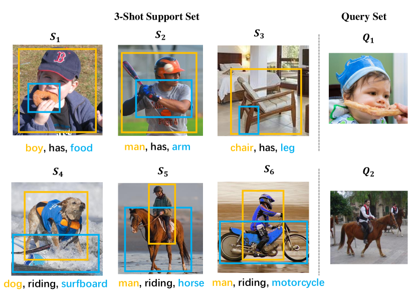
Figure 1: The illustration of FSSGG with 3-shots. For each predicate category, 3 support samples are provided with annotations (i.e. the bounding boxes and categories of subjects and objects, and predicate category). The target of FSSGG models is to detect the relation triplets in the query images.

In contrast, we humans are able to generalize the previous knowledge on new visual relationships quickly with only a few examples, and recognize them well. In this paper, we aim to imitate this human ability and equip SGG models with the transfer ability. Inspired by few-shot object detection [29, 30] and segmentation [36, 17], we propose a promising and important task: few-shot SGG (FSSGG). As shown in Figure 1, referring to a few annotated examples (i.e., support samples) of a novel predicate category, an ideal FSSGG model is expected to quickly capture the crucial clue for this predicate, recognize the relation triplets of it, and localize them in the target image (i.e., query image).

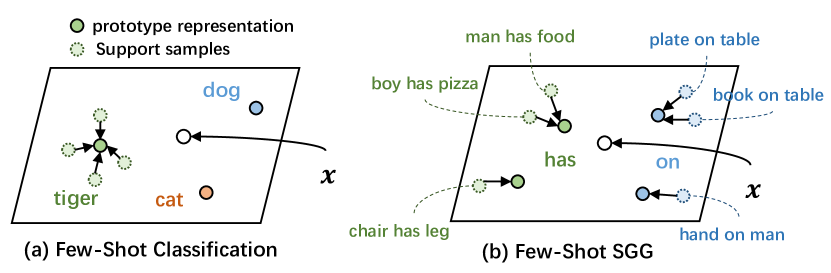
Figure 2: (a) The traditional metric-based method learns one prototype representation for each class in few-shot image classification. (b) Due to the multiple semantics of predicates in FSSGG, the predicate may have multiple prototypes in the latent space.

Currently, many approaches have been proposed to solve few-shot learning (FSL) tasks, such as object detection [6] and image classification [41]. And one of the most popular solutions is metric-based methods [12, 29, 30]. As shown in Figure 2(a), its basic idea is to project visual samples (e.g., $\boldsymbol{x}$) as points in a latent semantic space and devise a metric to calculate their distances to different category prototype representations, which are always assumed to be the centers of corresponding support points (i.e., one prototype for each category [29, 30, 24]). Although metric-based methods have achieved great success, naively applying them to FSSGG is non-trivial due to the intrinsic characteristics of visual relation concepts in SGG:

Firstly, polysemy is very common in the predicate categories, and each predicate category may have diverse semantics under different contexts. For example, as shown in Figure 1, the predicate has may not only mean possession relation between main body and individuals (e.g., $\left\langle\texttt{chair},\texttt{has},\texttt{leg}\right\rangle$) but also mean eating relation between human and food (e.g., $\left\langle\texttt{boy},\texttt{has},\texttt{food}\right\rangle$). This will lead to multiple semantic centers when all samples of one predicate are projected on the latent space (c.f., Figure 2(b)). Therefore, it is inadequate to represent each predicate category with only one prototype representation. Secondly, the relation triplets of the same predicate sometimes have totally distinct visual appearance under different subject-object pairs. For instance, the relation triplets of $\left\langle\texttt{man},\texttt{has},\texttt{arm}\right\rangle$ in $S_{2}$ and $\left\langle\texttt{chair},\texttt{has},\texttt{leg}\right\rangle$ in $S_{3}$ look irrelevant visually. This great variance of input signals increases the difficulty to build the projection of support samples into a concentrated point on the latent space, resulting in considerable confusion during inference as their distances from the query point may vary greatly.

In this paper, we propose a novel Decomposed Prototype Learning (DPL) for FSSGG, which can mitigate the mentioned issues. Specifically, for the first issue, in order to model multiple semantics of predicates, we construct a decomposable semantic space and represent each predicate as multiple semantic prototypes in this space. As the semantic meaning of each predicate is highly relevant to the subject-object pairs, we exploit the subject-object pair context of support samples to help us construct the semantic space for each predicate. However, due to the small number of support samples, it is difficult to catch enough information to build high-quality semantic representations. Inspired by recent prompt-tuning works, we devise learnable prompts to help us induce the knowledge of powerful pretrained VL models for deeper exploration of the predicate semantic space. Besides, in order to explore more novel compositions of subject-object context, we decompose the subject-object pairs and generate prototypes for subjects and objects separately (e.g., boy-has and has- food are regarded as two prototypes to be composable with other subject or object prototypes). We assign soft scores to each prototype for the input sample, and then exploit the attended prototype representations to enhance the final latent embedding of the sample. For the second issue, we devise an intelligent metric learner to estimate the confidence of each support sample for each query sample. Since each composition looks different, the metric learner will assign adaptive weights to each support sample by considering the relevance of their subject-object pairs to make more reliable predictions.

To better benchmark the new proposed Few-Shot SGG, we re-split the prevalent Visual Genome (VG) dataset [13] into 80 base predicate categories and 60 novel predicate categories to evaluate the transfer ability of the model on novel predicate categories. Meanwhile, the object categories are shared in both base and novel relation triplets.

We summarize our contributions as follows:

• We propose a new promising research task: FSSGG, which requires SGG models to transfer the knowledge quickly to novel predicates with only a few examples.

• We devise a decomposable prototype space to model multiple semantics of predicates, and equip it with the knowledge of powerful VL models. Besides, we propose an intelligent metric learner to adaptively assign confidence to each support for different query samples.

• To better benchmark FSSGG, we re-split VG dataset and evaluate several state-of-the-art FSL methods on the dataset for future research.

2 Related Work

Scene Graph Generation (SGG). SGG aims to predict visual relationship triplets between object pairs in an image. Recent SGG works mainly focus on three directions: 1) Model Architectures: Current mainstream SGG methods are mostly based on two-stage: they first detect all localized objects and subsequently predict their entity categories and pair-wise relationships. Usually, they focus on modeling global context information [38, 32, 37, 4], language priors [25, 38] and so on. Recently, several one-stage SGG works [19, 33] based on Transformer [35] have been proposed and achieved impressive performance. They generate the pairs of localized objects and their relationships simultaneously. 2) Unbiased SGG: Due to the long-tailed predicate distribution in the prevalent SGG datasets, unbiased SGG which aims to improve the performance of tail informative predicates has attracted considerable attention [31, 18]. 3) Weakly-supervised SGG: To overcome the limitation of expensive annotations, researchers proposed to solve SGG under weakly-supervised setting, i.e., using image-level annotations as supervision [39, 22]. In this work, we focus on transferring previous knowledge for novel predicate categories and propose a new promising task: FSSGG.

Few-Shot Learning (FSL). FSL has been widely explored in various scene understanding tasks to get rid of costly manual labeling efforts. It aims to learn valid knowledge about novel categories quickly with only a few reference samples. To achieve this goal, lots of creative solutions have been proposed. One of the most well-known paradigm of FSL is meta-learning, which can be further categorized into three groups: 1) Metric-based: Learning a projection function and measuring the similarity between query and support samples on the learned space [29, 30, 21, 20], which always assumes that each class has a prototype representation at the center of support points. 2) Memory-based: Designing models capable of quick adaptation to novel tasks with an external memory [2, 28]. 3) Optimization-based: Learning a good model initialization that enables the model to be adapted to novel tasks using a few optimization steps [16, 7]. Recently, some works begin to focus on prompt learning methods that design proper prompts for few-shot or zero-shot learning using large pretrained models [34, 1, 11, 10]. We share the core idea of metric-based meta-learning algorithms while focusing on SGG, i.e., the proposed learnable prototype space for learning compositional patterns across different predicate categories.

Prompt Learning. Prompt learning is an emerging technique to allow the large pre-trained models to be able to perform few-shot or even zero-shot learning on new scenarios by defining a new prompting function. With the emergence of large VL models like CLIP [27], prompt learning has been widely used in various tasks in the vision community, such as zero-shot image classification [27], object detection [5], and captioning [3]. Early works [26] just exploit fixed prompts to exploit the knowledge of VL models, and researchers found that model performance is highly related to the input prompts. However, the engineering of designing hand-crafted prompts is extremely time-consuming. To make it more efficient, recent works [41] attempt to model the prompts with a set of learnable vectors in continuous space and achieved great success. Currently, many excellent works [23, 41, 40, 8] based on task-specific prompt learning have been proposed. In this work, we devise learnable prompts to help us generate semantic prototypes (for both subject and object) of predicates.

3 Method

3.1 Problem Formulation

Given an image, SGG aims to not only detect the objects in the target image but also predict the predicate between them. In this paper, we focus on few-shot learning of SGG. Given a set of object category $\mathcal{C}$ and a set of predicate category $\mathcal{R}$, the predicate categories are split into the novel set $\mathcal{R}^{N}$ and the base set $\mathcal{R}^{B}$ (i.e., $\mathcal{R}=\mathcal{R}^{B}\cup\mathcal{R}^{N}$). The training set only includes samples of base categories. During evaluation, each predicate category $r\in\mathcal{R}$ is provided an annotated support example set $\mathcal{S}_{r}$ with $K$ shots (i.e., $K$ support images with only 1 annotated triplet for each predicate). And for each support triplet $\left\langle s,r,o\right\rangle\in\mathcal{S}_{r}$, it is provided with category annotations of subject and object $c_{s},c_{o}\in\mathcal{C}$, as well as the bounding boxes $b_{s},b_{o}$ of the object pairs. Given a query image $I$ and the support set of one category $r$, FSSGG aims to detect all the target relationship triplets belonging to the support category $r$ in the query image. Following the two-stage SGG pipeline, we first detect a set of proposals $\mathcal{B}$ with a pretrained object detector, and for each pair of proposal $b_{s},b_{o}\in\mathcal{B}$, we encode its embedding and compute similarity with each support triplet of $r$. To mimic the evaluation setting, the support set and query set is usually randomly sampled in one batch during training.

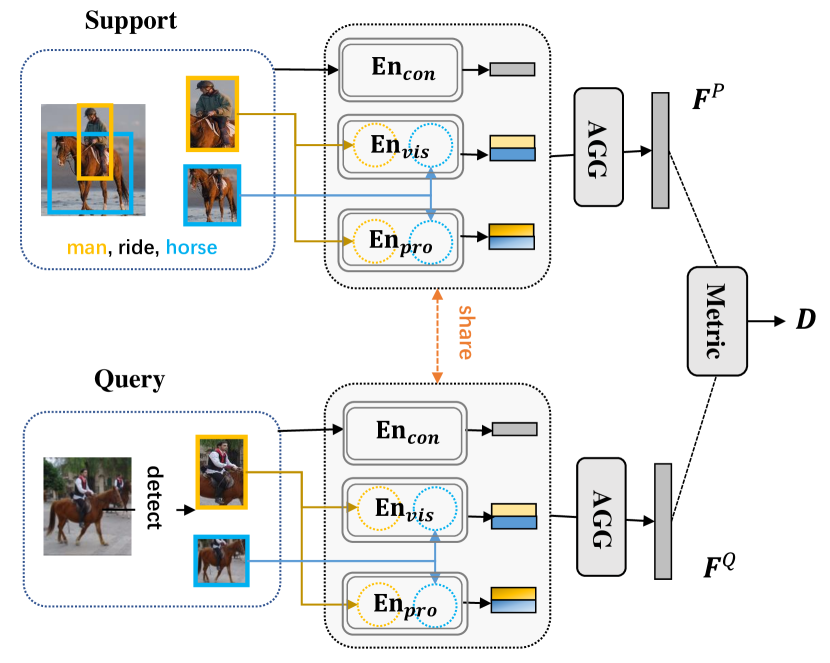
Figure 3: The pipeline of our method. We generate the representations for both query and support samples with a projection network and then estimate the distance between them by a metric learner.

3.2 Pipeline Overview

Following previous metric-based FSL works [29, 41, 6], we aim to construct a projection network to learn effective latent representations of visual relationships, as shown in Figure 3. Then, we measure the distance between the representations of the query and support samples with a metric learner to estimate whether they belong to the same category. To model useful information from multiple cues, our projection network contains a visual encoder, a context encoder, and a proposed prototype encoder.

Visual Encoder. Given a pair of proposals $b_{s}$ and $b_{o}$ in an image $I$, we extract the visual feature of each proposal with a visual encoder $\text{Enc}_{vis}$:

$$\mathbf{f}^{v}_{s}=\text{Enc}_{vis}\left(b_{s}\right),\quad\mathbf{f}^{v}_{o}=\text{Enc}_{vis}\left(b_{o}\right),$$ (1)

Context Encoder. As the predicate prediction for a pair of objects is highly relevant to the scene context information (e.g., spatial positions of objects and global information about other detected objects in the image), we follow previous SGG works and exploit a context encoder to extract contextual information in the image. Given an arbitrary context encoder $\text{Enc}_{con}$ (e.g., Motifs [38], VCTree [32]), we can obtain the context feature of one object pair $s$ and $o$:

$$\mathbf{f}^{con}_{s\rightarrow o}=\text{Enc}_{con}\left(I,b_{s},b_{o},\mathcal{B}_{/so}\right),$$ (2)

where $\mathcal{B}_{/so}$ is the set of other detected objects in image $I$.

Prototype Representation. To model multiple semantics of predicates, we devise a decomposed prototype encoder $\text{Enc}_{pro}$ to generate decomposed prototype representations for the input object pair $s$ and $o$:

$$\mathbf{f}^{pro}_{s\rightarrow o}=\text{Enc}_{pro}\left(b_{s},b_{o}\right),$$ (3)

and more details about $\text{Enc}_{pro}$ are explained in Sec 3.3.

Feature Aggregation. After obtaining these encoded features, we integrate them with an aggregator AGG:

$$\mathbf{F}_{s\rightarrow o}=\text{AGG}\left(\mathbf{f}^{v}_{s},\mathbf{f}^{v}_{o},\mathbf{f}^{con}_{s\rightarrow o},\mathbf{f}^{pro}_{s\rightarrow o}\right).$$ (4)

Here, we simply exploit a two-layer MLP as our aggregator, leaving other fancy operations as future work.

Metric Learning. After obtaining the representations of query sample $i$ (with object pair $\left\langle s,o\right\rangle$) and support triplet1 $j$, we compute their Euclidean distance following [29]:

$$d_{i,j}=\left\|\mathbf{F}^{Q}_{i}-\mathbf{F}^{P}_{j}\right\|^{2},$$ (5)

where $\mathbf{F}^{Q}_{i}$ and $\mathbf{F}^{P}_{j}$ are the final representations of sample $i$ and $j$ computed by Eq. (4). After that, the common policy is to average the distances between the query sample $i$ and all the support samples of category $r$ to get the final scores between $i$ and the category $r$. And the distance is:

$$d(i,r)=\frac{1}{|S_{r}|}\sum_{j\in S_{r}}d_{i,j}.$$ (6)

While in our method DPL, we will exploit an adaptive metric learner to compute the scores of query sample $i$ and the support category $r$. More details are in Sec 3.3.

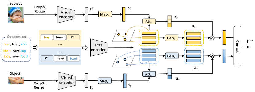
Figure 4: The overview of the construction process of our decomposed prototype representation. We first decompose the target predicate category into a set of prototype representations based on its support set. Given a query sample, we recombine the prototypes with adaptive weights by considering the subject-object pairs. The recombined feature is used to enhance the final representation of the query sample. The representation construction of support samples follows the same pipeline which is omitted in this figure.

3.3 Decomposed Prototype Learning

In this subsection, we will introduce the details of our proposed DRL paradigm. We first construct the decomposed semantic space for each predicate with the help of pretrained VL models. Then, we generate attended semantic prototype representations for each triplet sample to enhance its latent embedding. Lastly, we devise a metric learner to intelligently estimate the distance between query and support samples by assigning adaptive weights.

3.3.1 Prototype Generation

Prompt Tokens. Prompt tuning is an efficient way to transfer the knowledge of the large pretrained VL models into downstream tasks. In this paper, we introduce learnable prompts as indicators to help us construct the semantic space for each predicate with the power of VL models. As the semantics of one predicate are highly related to the subject-object context, we combine the subject and object category with the prompts to induce the semantic knowledge of predicates. To explore more compositions of subject-object context, we exploit the subjects and objects to generate prototypes separately.

Specifically, we first define the contextual prompt tokens $\mathbf{T}^{s}=[\mathbf{t}^{s}_{1},\cdots,\mathbf{t}^{s}_{L}]$ and $\mathbf{T}^{o}=[\mathbf{t}^{o}_{1},\cdots,\mathbf{t}^{o}_{L}]$ for the subject and object separately, and $L$ is the length of prompt tokens. Given a predicate category $r$ and its one support triplet $k$ with subject-object pairs $\left\langle s,o\right\rangle$, we exploit their annotated label words with our prompt tokens to construct our prompts:

$$\mathbf{p}^{s}_{k}=\left[\mathbf{W}[s];\mathbf{W}[r];\mathbf{T}^{s}\right],\quad\mathbf{p}^{o}_{k}=\left[\mathbf{T}^{o};\mathbf{W}[r];\mathbf{W}[o]\right],$$ (7)

where $\mathbf{W}[s]$ and $\mathbf{W}[o]$ are the category word embeddings for $s$ and $o$, respectively, and the $\mathbf{W}[r]$ is the category word embeddings for predicate $r$.

Prototype Generation. After obtaining all the composed prompts $\mathcal{P}$, we feed them into the text encoder of the VL model to extract the text embedding for each prompt:

$$\mathbf{h}^{s}_{k}=\text{Enc}_{txt}\left(\mathbf{p}^{s}_{k}\right),\quad\mathbf{h}^{o}_{k}=\text{Enc}_{txt}\left(\mathbf{p}^{o}_{k}\right),$$ (8)

where $\mathbf{p}^{s}_{k}\in\mathcal{P}^{s}$ and $\mathbf{p}^{o}_{k}\in\mathcal{P}^{o}$ are the generated prompt embeddings for the subject and object, respectively. The obtained text embeddings $\mathbf{h}^{s}_{k}\in\mathcal{H}^{s}$ and $\mathbf{h}^{o}_{k}\in\mathcal{H}^{o}$can be regarded as the extracted semantic knowledge from the VL model. Then, we generate the prototypes from the text embedding $\mathbf{h}_{k}$:

$$\mathbf{u}^{s}_{k}=\text{Gen}_{s}\left(\mathbf{h}^{s}_{k}\right),\quad\mathbf{u}^{o}_{k}=\text{Gen}_{o}\left(\mathbf{h}^{o}_{k}\right),$$ (9)

where $\text{Gen}_{s}$ and $\text{Gen}_{o}$ are two-layer MLPs for subject and object, respectively. And $\mathbf{u}_{k}^{s}\in\mathcal{U}^{s}$ and $\mathbf{u}_{k}^{o}\in\mathcal{U}^{o}$ are the generated prototypes.

3.3.2 Decomposed Prototype Representation

Each triplet sample of the predicate may have different semantics due to different subject-object pairs. Thus, we assign adaptive weights to each prototype for each sample. Given a query sample $i$ with subject $s$ and object $o$, we first project the encoded visual feature $\mathbf{f}^{v}_{s}$ and $\mathbf{f}^{v}_{o}$ (computed from Eq. (1)) into the prototype space:

$$\mathbf{v}_{s}=\text{Map}_{s}\left(\mathbf{f}^{v}_{s}\right),\quad\mathbf{v}_{o}=\text{Map}_{o}\left(\mathbf{f}^{v}_{o}\right),$$ (10)

where $\text{Map}_{s}$ and $\text{Map}_{o}$ are both two-layer MLPs.

Then, we compute the similarity score of each text embedding of the prototype $k$ and visual embedding of query sample $i$ for both subject and object:

$$a_{k}=\text{Att}\left(\mathbf{v}\odot\mathbf{h}_{k}\right),$$ (11)

where Att is a two-layer MLP, $\odot$ is element-wise production, and $N$ is the number of prototypes, we omit the subscripts for subject and object here. We normalize the scores $a_{*}$ with softmax to get the attention score $\tilde{a}_{*}$.

Later, we aggregate the generated prototype $\tilde{\mathbf{u}}$ for subject and object with normalized attention scores $\tilde{a}$:

$$\tilde{\mathbf{u}}^{s}={\sum_{k=1}^{|\mathcal{P}|}}\tilde{a}^{s}_{k}\mathbf{u}^{s}_{k},\quad\tilde{\mathbf{u}}^{o}={\sum_{k=1}^{|\mathcal{P}|}}\tilde{a}^{o}_{k}\mathbf{u}^{o}_{k},$$ (12)

where $|\mathcal{P}|$ is the number of prototypes. After that, we concatenate the prototype features for each sample:

$$\mathbf{f}^{pro}=[\tilde{\mathbf{u}}^{s};\tilde{\mathbf{u}}^{o}],$$ (13)

and we will enhance the final representation of query sample $i$ with generated $\mathbf{f}^{pro}$.

3.3.3 Metric Learner

After obtaining the distance between the query sample and each support sample, a naturally exploited approach in previous works is to average these distances. However, as the visual appearance of the relationship triplets differs greatly under different subject-object pairs, the predictions computed by averaging the distance in Eq. (6) will be disturbed by samples with large differences, resulting in wrong predictions. Therefore, given a query sample $i$, we propose to pay higher attention to the support samples with more similar subject-object pairs with $i$ when making predictions. Here, we model the similarity between subjects and objects with the text embeddings of pretrained VL models.

We first send the predicted category of the subject and object with a pre-defined prompt into the text encoder of the VL model and get text features. Then, we compute the similarity of subject and object text embeddings between the query sample and each support sample. Last, we multiply the scores to get the final weights:

$$\hat{e}_{i,j}=e^{s}_{i,j}*e^{o}_{i,j},$$ (14)

where $e^{s}_{i,j}$ and $e^{o}_{i,j}$ are the similarity scores for the subject and object between query sample $i$ and support sample $j$. And we normalize $\hat{e}_{i,*}$ with softmax to get $\tilde{e}_{i,*}$.

The final distance between query sample $i$ and support samples of predicate $r$ is combined as:

$$\tilde{d}(i,r)=\sum_{j\in\mathcal{S}_{r}}\tilde{e}_{i,j}d_{i,j},$$ (15)

where $\mathcal{S}_{r}$ is the support set of predicate category $r$.

3.4 Model Training

During training, we randomly sample the categories $R_{b}$ in one batch, and for each category $r$, we randomly select a part of its positive samples as the support set, while the rest positives are regarded as query samples. For each query sample $i$ in batch $\mathcal{D}_{b}$, we compute the loss by its distance with the positive $r$ and negative categories:

$$\mathcal{L}_{rel}=-\sum_{i\in\mathcal{D}_{b}}\left(\text{log}\frac{\text{exp}(-\tilde{d}(i,r))}{{\textstyle\sum_{j\in\mathcal{R}_{b}}}\text{exp}(-\tilde{d}(i,j))}\right).$$ (16)

To train the prototype space, we expect the predictions only with the prototype features can work as well as the final aggregated features. Therefore, we exploit Kullback Leibler (KL) divergence loss to make the output distribution of prototype features close to the final output:

$$\mathcal{L}_{kl}=\sum_{i\in\mathcal{D}_{b}}\text{KL}(\hat{\mathbf{y}}_{i}||\mathbf{y}^{pro}_{i}),$$ (17)

where $\mathbf{y}^{pro}$ is the output distribution calculated only by prototype features $\mathbf{f}^{pro}$, and $\hat{\mathbf{y}}_{i}$ is the output distribution with final aggregated representations $\mathbf{F}$.

The total training loss of our method is as follows:

$$\mathcal{L}=\mathcal{L}_{rel}+\mathcal{L}_{kl}+\mathcal{L}_{obj},$$ (18)

where $\mathcal{L}_{obj}$ is cross entropy loss for object classification.

Method Encoder 1-shot (mR) 5-shot (mR) 10-shot (mR) Base Novel Base Novel Base Novel @20 / 50 / 100 @20 / 50 / 100 @20 / 50 / 100 @20 / 50 / 100 @20 / 50 / 100 @20 / 50 / 100 Predcls Baseline^† Motifs 4.7 / 8.9 / 12.0 0.0 / 0.1 / 0.2 4.2 / 7.7 / 11.3 0.4 / 0.7 / 1.1 4.3 / 7.8 / 11.4 1.6 / 2.4 / 2.9 ProtoNet [29] 4.5 / 7.0 / 9.1 1.7 / 2.7 / 3.3 8.6 / 12.1 / 15.0 3.0 / 3.9 / 4.4 8.6 / 12.2 / 15.3 3.6 / 4.6 / 5.3 RelationNet [30] 2.8 / 5.6 / 8.4 1.4 / 2.0 / 2.4 6.3 / 10.7 / 14.4 2.0 / 2.8 / 3.6 7.8 / 11.8 / 14.9 2.3 / 3.3 / 4.3 CoOp [41] 0.2 / 0.5 / 1.0 0.8 / 1.3 / 1.8 0.2 / 0.5 / 1.0 1.6 / 2.6 / 3.8 0.3 / 0.7 / 1.3 2.3 / 3.8 / 4.9 CSC [41] 0.2 / 0.6 / 1.1 1.8 / 2.7 / 3.4 0.2 / 0.6 / 1.2 2.9 / 4.7 / 6.0 0.3 / 0.7 / 1.3 3.4 / 5.1 / 6.3 DPL (Ours) 6.9 / 10.2 / 12.8 2.6 / 3.2 / 3.9 10.2 / 15.4 / 18.6 4.8 / 5.9 / 6.6 10.9 / 15.9 / 19.5 5.1 / 6.3 / 6.9 Baseline^† VCTree 4.4 / 8.1 / 12.1 0.1 / 0.2 / 0.3 4.4 / 8.1 / 12.1 0.5 / 0.8 / 1.2 4.4 / 8.3 / 12.4 1.4 / 2.1 / 2.6 ProtoNet [29] 4.1 / 6.4 / 9.0 1.5 / 2.2 / 2.8 9.3 / 12.6 / 15.4 3.2 / 4.4 / 5.1 8.9 / 12.6 / 15.6 3.5 / 4.8 / 5.6 RelationNet [30] 4.6 / 7.9 / 11.1 2.0 / 2.7 / 3.0 7.6 / 11.6 / 14.7 2.1 / 2.7 / 3.1 7.3 / 10.4 / 13.1 2.2 / 3.3 / 4.1 CoOp [41] 0.2 / 0.5 / 1.1 0.6 / 1.1 / 1.6 0.4 / 0.7 / 1.5 1.5 / 2.9 / 3.9 0.2 / 0.6 / 1.5 2.4 / 3.7 / 5.0 CSC [41] 0.2 / 0.6 / 1.2 2.4 / 3.3 / 4.2 0.3 / 0.6 / 1.1 3.3 / 4.6 / 5.9 0.2 / 0.6 / 1.7 4.8 / 6.3 / 7.5 DPL (Ours) 7.5 / 10.3 / 12.2 3.0 / 3.8 / 4.3  11.2 / 16.6 / 20.0  5.4 / 6.6 / 7.2  10.8 / 16.3 / 20.0 5.2 / 6.4 / 7.1 SGCls Baseline^† Motifs 3.0 / 4.4 / 5.8 0.0 / 0.0 / 0.1 2.9 / 4.4 / 5.7 0.1 / 0.2 / 0.3 3.0 / 4.5 / 5.7 0.6 / 0.8 / 1.0 ProtoNet [29] 2.1 / 3.1 / 3.8 0.5 / 0.8 / 1.0 4.1 / 5.2 / 5.9 1.1 / 1.3 / 1.5 3.9 / 5.2 / 6.1 1.4 / 1.7 / 1.9 RelationNet [30] 1.9 / 2.9 / 3.5 0.7 / 0.9 / 1.1 3.4 / 4.5 / 5.3 1.0 / 1.2 / 1.3 3.7 / 5.0 / 5.7 1.1 / 1.4 / 1.5 CoOp [41] 0.2 / 0.4 / 0.6 0.2 / 0.2 / 0.3 0.3 / 0.6 / 1.0 0.5 / 0.8 / 0.9 0.4 / 0.7 / 1.3 0.9 / 1.2 / 1.6 CSC [41] 0.1 / 0.2 / 0.3 0.2 / 0.2 / 0.3 0.3 / 0.7 / 1.0 0.8 / 1.2 / 1.5 0.4 / 0.8 / 1.3 1.1 / 1.6 / 1.9 DPL (Ours) 2.8 / 3.7 / 4.4 0.9 / 1.2 / 1.3 4.5 / 5.9 / 7.0 1.6 / 1.9 / 2.1 4.8 / 6.5 / 7.4 1.6 / 1.9 / 2.2 SGDet Baseline^† Motifs 1.4 / 1.8 / 2.1 0.0 / 0.0 / 0.1 1.5 / 1.9 / 2.1 0.2 / 0.3 / 0.4 1.5 / 1.9 / 2.1 0.2 / 0.4 / 0.4 ProtoNet [29] 0.7 / 0.9 / 1.1 0.4 / 0.4 / 0.5 1.3 / 1.5 / 2.0 0.5 / 0.7 / 0.7 1.5 / 1.9 / 2.2 0.5 / 0.6 / 0.7 RelationNet [30] 0.8 / 1.0 / 1.1 0.4 / 0.5 / 0.5 1.3 / 1.6 / 2.0 0.4 / 0.4 / 0.5 1.3 / 1.6 / 1.9 0.5 / 0.6 / 0.6 CoOp [41] 0.2 / 0.3 / 0.4 0.0 / 0.1 / 0.1 0.3 / 0.5 / 0.7 0.2 / 0.3 / 0.4 0.6 / 0.8 / 1.0 0.4 / 0.4 / 0.5 CSC [41] 0.1 / 0.2 / 0.4 0.2 / 0.3 / 0.4 0.4 / 0.6 / 0.7 0.3 / 0.4 / 0.5 0.7 / 0.9 / 1.1 0.5 / 0.6 / 0.7 DPL (Ours) 0.9 / 1.1 / 1.2 0.4 / 0.5 / 0.6 1.5 / 1.7 / 2.1 0.5 / 0.6 / 0.7 1.6 / 2.1 / 2.3 0.5 / 0.7 / 0.8

Table 1: FSSGG performance (%) comparison on mR@K. We mainly report the mR@K scores of all the methods on both Base and Novel splits. VCTree [32] and Motifs [38] are two popular SGG models exploited as context encoders. ^† For the baseline results, we added the support samples for Novel (unknown in the training stage for all other baselines) and Base categories into training data and train models in a conventional fully-supervised way.

4 Experiments

4.1 Experimental Settings

Datasets. We conducted all experiments on the most prevalent SGG dataset: Visual Genome (VG) [13]. To benchmark FSSGG, we re-split VG, and set $80$ common predicate categories as base categories and $60$ rare predicate categories as novel categories. As for the object categories, we selected the most common $247$ object categories, and they are shared in both training and test sets. For each predicate category, we randomly split $K$-shot from its samples as its support samples in the test set. The triplet samples annotated with novel predicate in the test set are called Novel split, and the triplet samples annotated with base predicate are called Base split. In experiment, we set $K$ as $1$, $5$ and $10$, respectively. In summary, there are 11K test images and 78K training images.

Tasks. Following SGG works, We evaluated FSSGG on three tasks: 1) Predicate Classification (PredCls): Given ground-truth object bboxes and class labels, the model is required to predict the predicate class of pairwise objects. 2) Scene Graph Classification (SGCls): Given ground-truth object bboxes, the model is required to predict both object classes and predicate classes of pairwise objects. 3) Scene Graph Detection (SGDet): Given an image, the model is required to detect object bboxes, and predict object classes and predicate classes of pairwise objects.

Evaluation Metrics. To avoid the major influence of common categories on performance and evaluate each category equally, following recent works [31], we mainly reported the performance on mean Recall@K (mR@K) which is the average of recall scores computed for each category separately. Following previous FSL works [9, 14], we reported mR@K performance on both Novel and Base splits.

Training Details. To mimic the evaluation setting, we randomly generated the support set and query set from training data in a batch. For each batch, we selected $N_{b}$ categories, and split its positive samples into support samples and query samples randomly. The number of sampled categories $N_{b}$, query, and support samples for each predicate are set differently according to the batch data. We set the ratio of foreground samples and background samples as 1:2. In the experiment, we set the number of tokens for each prompt as $24$ for all prompt-based experiments. We exploited pretrained CLIP [27] as our VL model in all our prompt-based experiments. In the SGDet task, we exploited a Faster R-CNN detector pretrained on OpenImage [15] to extract the general proposals in the images as weakly-supervised SGG [22].

4.2 Model Comparison

Baselines. To better evaluate our DPL, we compared it with a set of state-of-the-art FSL methods: 1) Metric-base Methods: ProtoNet [29] and RelationNet [30]. They both generate the latent embeddings of the query sample and support sample with the same network, and estimate their similarity by computing Euclidean distance and a trainable metric net, respectively. 2) Prompt-based Methods: CoOp [41] and CSC [41]. They both introduce learnable prompts and exploit CLIP to extract text embeddings of the target category, and then compute the cosine similarity scores with the visual embeddings of each sample. The difference is that CoOp sets global prompts shared across all categories while CSC set specific prompts for each category. Following [41], we fine-tuned models CoOp and CSC on the $K$-shot support set. For fair comparisons, we also pretrained them on base training data in advance. For ProtoNet and RelationNet, we applied the same sampling strategy with DPL. We exploited SGG models VCTree [32] and Motifs [38] as context encoders and reported results in Table 1.

	1-shot	5-shot	10-shot
	@50 / 100	@50 / 100	@50 / 100
Baseline	2.7 / 3.3	3.9 / 4.4	4.6 / 5.3
+Fixed	1.6 / 2.4	2.6 / 3.5	2.8 / 4.0
+Learnable	3.2 / 3.9	5.9 / 6.6	6.3 / 6.9

Table 2: MR@K performance (%) of decomposed prototype representation with the fixed and learnable prompts on Novel split.

Results Analysis. From Table 1, we can find the following observations: 1) Our method achieves state-of-the-art performance on both Novel and Base splits under almost all the settings. Even in the challenging $1$-shot setting, it performs excellently. 2) The two prompt-based methods perform well on the Novel split but fail on the Base split. That may be due to the fact that the VL models like CLIP are mostly pretrained on image-caption pairs based on contrastive learning paradigm and they mainly focus on more concrete visual concepts (e.g., object) or fine-grained semantic concepts (e.g., action relationships). They are not sensitive to spatial relationships (e.g. on and in), which are mostly split into the Base categories. Compared to CoOp, CSC performs better on novel splits which is consistent with the conclusion in [41] that CSC works better on some fine-grained categories with specific prompts for each category. While different from CSC, our DPL devises a compositional prompt learning paradigm and exploits a small number of prompts shared across categories which can uncover the hidden semantic knowledge of relationship triplets in VL models, providing great improvements on both novel and base splits. 3) The performance of two metric-based methods is excellent on both Base and Novel splits and even exceeds the Base split performance of traditional classification paradigm (i.e. Baseline in Table 1) on $5$-shot and $10$-shot. However, they are still inferior to our DPL method. That is due to that the previous metric-based methods are not tailored to relationship triplets learning and ignore the compositional structure of the relationship triplets. In contrast, our decomposable prototype space and adaptive metric learner explore this compositional knowledge in subjects and objects.

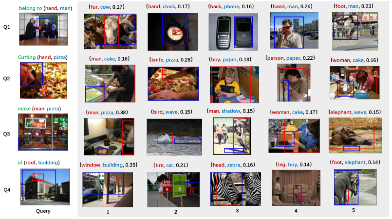
Figure 5: Visualization of assigned weights on $5$-shot of support samples. The first column displays the query triplets and the target predicates (highlighted in green). The other columns display the support triplets and their assigned weights by our metric learner. The subjects and objects are drawn in red and blue boxes respectively.

4.3 Ablation Study

In this section, we conducted a set of ablation studies on the two proposed modules: decomposed prototype representation and adaptive metric learner.

Study of Decomposed Prototype Representation. In this part, we mainly analyze the effectiveness of our decomposed prototype representation. We first removed the decomposed prototype representation to observe the performance (i.e., Baseline in Table 2). We also devised an experiment with fixed prompts (removing the learnable prompt tokens) to extract the semantic embeddings to show the superiority of our learnable prompts. We reported the mR@K performance on Novel split in Table 2 and set $K$ as $1$, $5$, and $10$, respectively. From the table, we can see that our learnable prompts bring great improvement compared to the baseline, which verifies the effectiveness of our DPL module. In contrast, exploiting semantic knowledge with fixed prompts harms the model’s performance. This verifies the difficulty of semantic prototype modeling and directly exploiting hand-crafted prompts is non-trivial. In comparison, our devised learnable prompts are able to induce useful knowledge of the VL model and bring benefits to the model.

	1-shot	5-shot	10-shot
	@50 / 100	@50 / 100	@50 / 100
Baseline	2.7 / 3.3	3.9 / 4.4	4.6 / 5.3
+Average	3.6 / 4.0	4.7 / 5.3	5.3 / 5.9
+Re-weight	3.2 / 3.9	5.9 / 6.6	6.3 / 6.9

Table 3: Ablation study of the metric learner on the Novel split.

Study of Metric Learner. To verify the effectiveness of our metric learner, we removed the re-weighting strategy and averaged the distance from each support sample to make final predictions (i.e., Average in Table 3). Benefiting from our decomposed prototype representation module, the average strategy achieves better performance compared to the baseline, as shown in Table 3. However, its performance drops a lot compared to the re-weighting strategy under the settings of $5$-shot and $10$-shot. This is because that the average strategy ignores the difference among support samples when estimating their distance with query samples.

Case Study. To show how our metric learner works, we randomly selected some query triplets and visualized their weights assigned to the support samples during the inference in Figure 5. We have the following findings: 1) The visual appearances of support samples for one predicate vary greatly under different subject-object compositions. 2) For each query triplet, our metric learner tends to assign higher attention weights to more reliable support samples which have relevant subject-object pairs with the query sample, thus helping our model make more accurate predictions.

5 Conclusion

In this paper, we proposed a promising and important research task: Few-shot Scene Graph Generation (FSSGG), which requires SGG models to be able to recognize novel predicate categories quickly with only a few samples. Different from existing FSL tasks, the multiple semantics and great variance of the visual appearance of predicate categories make FSSGG non-trivial. To this end, we devised a novel Decomposable Prototype Learning (DPL). Specifically, we introduced learnable prompts to model multiple semantics of predicates with the help of pretrained VL models and adaptively assigned weights to each support sample by considering the subject-object compositions. To better benchmark FSSGG, we re-splited the prevalent VG dataset and evaluated several FSL methods on the new split for future research. We hope this work can inspire and attract FSL research on more challenging scene understanding tasks.

References

- [1] Jean-Baptiste Alayrac, Jeff Donahue, Pauline Luc, Antoine Miech, Iain Barr, Yana Hasson, Karel Lenc, Arthur Mensch, Katherine Millican, Malcolm Reynolds, et al. Flamingo: a visual language model for few-shot learning. In NeurIPS, 2022.
- [2] Qi Cai, Yingwei Pan, Ting Yao, Chenggang Yan, and Tao Mei. Memory matching networks for one-shot image recognition. In CVPR, pages 4080–4088, 2018.
- [3] Jun Chen, Han Guo, Kai Yi, Boyang Li, and Mohamed Elhoseiny. Visualgpt: Data-efficient adaptation of pretrained language models for image captioning. In CVPR, pages 18030–18040, 2022.
- [4] Long Chen, Hanwang Zhang, Jun Xiao, Xiangnan He, Shiliang Pu, and Shih-Fu Chang. Counterfactual critic multi-agent training for scene graph generation. In ICCV, pages 4613–4623, 2019.
- [5] Yu Du, Fangyun Wei, Zihe Zhang, Miaojing Shi, Yue Gao, and Guoqi Li. Learning to prompt for open-vocabulary object detection with vision-language model. In CVPR, pages 14084–14093, 2022.
- [6] Qi Fan, Wei Zhuo, Chi-Keung Tang, and Yu-Wing Tai. Few-shot object detection with attention-rpn and multi-relation detector. In CVPR, pages 4013–4022, 2020.
- [7] Chelsea Finn, Pieter Abbeel, and Sergey Levine. Model-agnostic meta-learning for fast adaptation of deep networks. In ICML, pages 1126–1135. PMLR, 2017.
- [8] Kaifeng Gao, Long Chen, Hanwang Zhang, Jun Xiao, and Qianru Sun. Compositional prompt tuning with motion cues for open-vocabulary video relation detection. In ICLR, 2023.
- [9] Spyros Gidaris and Nikos Komodakis. Dynamic few-shot visual learning without forgetting. In CVPR, pages 4367–4375, 2018.
- [10] Yuxian Gu, Xu Han, Zhiyuan Liu, and Minlie Huang. Ppt: Pre-trained prompt tuning for few-shot learning. arXiv, 2021.
- [11] Tao He, Lianli Gao, Jingkuan Song, and Yuan-Fang Li. Towards open-vocabulary scene graph generation with prompt-based finetuning. In ECCV, pages 56–73. Springer, 2022.
- [12] Junsik Kim, Tae-Hyun Oh, Seokju Lee, Fei Pan, and In So Kweon. Variational prototyping-encoder: One-shot learning with prototypical images. In CVPR, pages 9462–9470, 2019.
- [13] Ranjay Krishna, Yuke Zhu, Oliver Groth, Justin Johnson, Kenji Hata, Joshua Kravitz, Stephanie Chen, Yannis Kalantidis, Li-Jia Li, David A Shamma, et al. Visual genome: Connecting language and vision using crowdsourced dense image annotations. IJCV, 123:32–73, 2017.
- [14] Anna Kukleva, Hilde Kuehne, and Bernt Schiele. Generalized and incremental few-shot learning by explicit learning and calibration without forgetting. In ICCV, pages 9020–9029, 2021.
- [15] Alina Kuznetsova, Hassan Rom, Neil Alldrin, Jasper Uijlings, Ivan Krasin, Jordi Pont-Tuset, Shahab Kamali, Stefan Popov, Matteo Malloci, Alexander Kolesnikov, et al. The open images dataset v4: Unified image classification, object detection, and visual relationship detection at scale. IJCV, 128(7):1956–1981, 2020.
- [16] Kwonjoon Lee, Subhransu Maji, Avinash Ravichandran, and Stefano Soatto. Meta-learning with differentiable convex optimization. In CVPR, pages 10657–10665, 2019.
- [17] Gen Li, Varun Jampani, Laura Sevilla-Lara, Deqing Sun, Jonghyun Kim, and Joongkyu Kim. Adaptive prototype learning and allocation for few-shot segmentation. In CVPR, pages 8334–8343, 2021.
- [18] Lin Li, Long Chen, Yifeng Huang, Zhimeng Zhang, Songyang Zhang, and Jun Xiao. The devil is in the labels: Noisy label correction for robust scene graph generation. In CVPR, pages 18869–18878, 2022.
- [19] Rongjie Li, Songyang Zhang, and Xuming He. Sgtr: End-to-end scene graph generation with transformer. In CVPR, pages 19486–19496, 2022.
- [20] Wenbin Li, Lei Wang, Jinglin Xu, Jing Huo, Yang Gao, and Jiebo Luo. Revisiting local descriptor based image-to-class measure for few-shot learning. In CVPR, pages 7260–7268, 2019.
- [21] Wenbin Li, Jinglin Xu, Jing Huo, Lei Wang, Yang Gao, and Jiebo Luo. Distribution consistency based covariance metric networks for few-shot learning. In AAAI, pages 8642–8649, 2019.
- [22] Xingchen Li, Long Chen, Wenbo Ma, Yi Yang, and Jun Xiao. Integrating object-aware and interaction-aware knowledge for weakly supervised scene graph generation. In ACM MM, pages 4204–4213, 2022.
- [23] Xiang Lisa Li and Percy Liang. Prefix-tuning: Optimizing continuous prompts for generation. pages 4582–4597, 2021.
- [24] Jinlu Liu, Liang Song, and Yongqiang Qin. Prototype rectification for few-shot learning. In ECCV, pages 741–756. Springer, 2020.
- [25] Cewu Lu, Ranjay Krishna, Michael Bernstein, and Li Fei-Fei. Visual relationship detection with language priors. In ECCV, pages 852–869. Springer, 2016.
- [26] Sauradip Nag, Xiatian Zhu, Yi-Zhe Song, and Tao Xiang. Zero-shot temporal action detection via vision-language prompting. In ECCV, pages 681–697. Springer, 2022.
- [27] Alec Radford, Jong Wook Kim, Chris Hallacy, Aditya Ramesh, Gabriel Goh, Sandhini Agarwal, Girish Sastry, Amanda Askell, Pamela Mishkin, Jack Clark, et al. Learning transferable visual models from natural language supervision. In ICML, pages 8748–8763. PMLR, 2021.
- [28] Adam Santoro, Sergey Bartunov, Matthew Botvinick, Daan Wierstra, and Timothy Lillicrap. Meta-learning with memory-augmented neural networks. In ICML, pages 1842–1850. PMLR, 2016.
- [29] Jake Snell, Kevin Swersky, and Richard Zemel. Prototypical networks for few-shot learning. In NeurIPS, volume 30, 2017.
- [30] Flood Sung, Yongxin Yang, Li Zhang, Tao Xiang, Philip HS Torr, and Timothy M Hospedales. Learning to compare: Relation network for few-shot learning. In CVPR, pages 1199–1208, 2018.
- [31] Kaihua Tang, Yulei Niu, Jianqiang Huang, Jiaxin Shi, and Hanwang Zhang. Unbiased scene graph generation from biased training. In CVPR, pages 3716–3725, 2020.
- [32] Kaihua Tang, Hanwang Zhang, Baoyuan Wu, Wenhan Luo, and Wei Liu. Learning to compose dynamic tree structures for visual contexts. In CVPR, pages 6619–6628, 2019.
- [33] Yao Teng and Limin Wang. Structured sparse r-cnn for direct scene graph generation. In CVPR, pages 19437–19446, 2022.
- [34] Maria Tsimpoukelli, Jacob L Menick, Serkan Cabi, SM Eslami, Oriol Vinyals, and Felix Hill. Multimodal few-shot learning with frozen language models. In NeurIPS, volume 34, pages 200–212, 2021.
- [35] Ashish Vaswani, Noam Shazeer, Niki Parmar, Jakob Uszkoreit, Llion Jones, Aidan N Gomez, Łukasz Kaiser, and Illia Polosukhin. Attention is all you need. In NeurIPS, volume 30, 2017.
- [36] Kaixin Wang, Jun Hao Liew, Yingtian Zou, Daquan Zhou, and Jiashi Feng. Panet: Few-shot image semantic segmentation with prototype alignment. In ICCV, pages 9197–9206, 2019.
- [37] Jianwei Yang, Jiasen Lu, Stefan Lee, Dhruv Batra, and Devi Parikh. Graph r-cnn for scene graph generation. In ECCV, pages 670–685, 2018.
- [38] Rowan Zellers, Mark Yatskar, Sam Thomson, and Yejin Choi. Neural motifs: Scene graph parsing with global context. In CVPR, pages 5831–5840, 2018.
- [39] Yiwu Zhong, Jing Shi, Jianwei Yang, Chenliang Xu, and Yin Li. Learning to generate scene graph from natural language supervision. In ICCV, pages 1823–1834, 2021.
- [40] Kaiyang Zhou, Jingkang Yang, Chen Change Loy, and Ziwei Liu. Conditional prompt learning for vision-language models. In CVPR, pages 16816–16825, 2022.
- [41] Kaiyang Zhou, Jingkang Yang, Chen Change Loy, and Ziwei Liu. Learning to prompt for vision-language models. IJCV, 130(9):2337–2348, 2022.