Revisiting Realistic Test-Time Training: Sequential Inference and Adaptation by Anchored Clustering Regularized Self-Training

Abstract

Deploying models on target domain data subject to distribution shift requires adaptation. Test-time training (TTT) emerges as a solution to this adaptation under a realistic scenario where access to full source domain data is not available, and instant inference on the target domain is required. Despite many efforts into TTT, there is a confusion over the experimental settings, thus leading to unfair comparisons. In this work, we first revisit TTT assumptions and categorize TTT protocols by two key factors. Among the multiple protocols, we adopt a realistic sequential test-time training (sTTT) protocol, under which we develop a test-time anchored clustering (TTAC) approach to enable stronger test-time feature learning. TTAC discovers clusters in both source and target domains and matches the target clusters to the source ones to improve adaptation. When source domain information is strictly absent (i.e. source-free) we further develop an efficient method to infer source domain distributions for anchored clustering. Finally, self-training (ST) has demonstrated great success in learning from unlabeled data and we empirically figure out that applying ST alone to TTT is prone to confirmation bias. Therefore, a more effective TTT approach is introduced by regularizing self-training with anchored clustering, and the improved model is referred to as TTAC++. We demonstrate that, under all TTT protocols, TTAC++ consistently outperforms the state-of-the-art methods on five TTT datasets, including corrupted target domain, selected hard samples, synthetic-to-real adaptation and adversarially attacked target domain. We hope this work will provide a fair benchmarking of TTT methods, and future research should be compared within respective protocols.

1 Introduction

The recent success in deep learning is attributed to the availability of large labeled data [1, 2, 3] and the assumption of i.i.d. between training and test datasets. Such assumptions could be violated when testing data features a drastic difference from the training data, e.g. training on synthetic images and test on real ones, or training on clean samples and test on corrupted ones. This situation is often referred to as domain shift [4, 5, 6]. To tackle this issue, domain adaptation (DA) [7] emerges and the labeled training data and unlabeled testing data are often referred to as source and target data/domains respectively. The existing DA works either require the access to both source and target domain data during training [8, 9, 10] or training on multiple domains simultaneously [11]. The former approaches render the methods restrictive to limited scenarios where source domain data is always available during adaptation while the latter ones are computationally more expensive.

To alleviate the dependence on source domain data, which may be inaccessible due to privacy issues or storage overhead, source-free domain adaptation (SFDA) emerges which handles DA on target data without access to source data [12, 13, 14, 15, 16]. SFDA is often achieved through self-training [12, 17], self-supervised learning [16, 18] or introducing prior knowledge [12] and it requires multiple training epochs on the full target dataset to allow model convergence. Despite easing the dependence on source data, SFDA has major drawbacks in a more realistic domain adaptation scenario where test data arrives in a stream and inference or prediction must be taken instantly, and this setting is often referred to as test-time training (TTT) or adaptation (TTA) [19, 20, 21, 16, 22, 23]. Despite the attractive feature of adaption at test time, we notice a confusion of what defines a test-time training and as a result comparing apples and oranges happens frequently in the community. In this work, we first categorize TTT by two key factors after summarizing various definitions made in existing works. First, under a realistic TTT setting, test samples are sequentially streamed and predictions should be made instantly upon the arrival of a new test sample. More specifically, the prediction of test sample $x_{T}$, arriving at time stamp $T$, should not be affected by any subsequent samples, $\{x_{t}\}_{t=T+1\cdots\infty}$. The sequential protocol widely exists in many real-world application. For example, in video surveillance, cameras are expected to function instantly after installment and adaptation to target domain must be carried out on-the-fly. Throughout this work, We refer to the sequential streaming setting as the one-pass adaptation protocol and any other protocols violating this assumption are referred to as multi-pass adaptation (model may be updated on all test data for multiple epochs before inference). Second, we notice some recent works must modify source domain training loss, e.g. by introducing additional self-supervised branch, to allow more effective TTT [19, 16]. This will introduce additional overhead in the deployment of TTT because re-training on some source dataset, e.g. ImageNet, is computationally expensive. Thus, we distinguish methods by whether source domain training objective is modified or not.

In this work, we aim to tackle on the most realistic TTT protocol, i.e. one-pass test time training with no modifications to training objective. We refer to this new TTT protocol as sequential test time training (sTTT). The proposed setting is similar to TTA proposed in [20] except for not restricting access to a light-weight distribution information from the source domain. We believe having access to distribution information, e.g. distributions’ mean and covariance, in the source domain is a realistic assumption for two reasons. First, the objective of TTT is efficient adaptation at test time, this assumption only requires storing the means and covariance matrices which are memory efficient. Moreover, feature distribution information will not pose any threat to privacy leakage as inverting backbone network, e.g. CNN, is known to be very challenging [24]. Nevertheless, we are aware that under certain scenarios source domain distribution information is not always available for test-time training, i.e. source-free test-time training. Such a situation could happen when source distribution is not recorded during training, or model is trained through federated learning where access to the whole source data is prohibited [25]. A robust TTT method should therefore be versatile and still function well in the absence of source domain distribution information.

In this work, we propose four techniques to enable efficient and accurate sTTT regardless the availability of source domain distribution information. i) We are inspired by the recent progresses in unsupervised domain adaptation [26] that encourages testing samples to form clusters in the feature space. However, separately learning to cluster in the target domain without regularization from source domain does not guarantee improved adaptation [26]. To overcome this challenge, we identify clusters in both the source and target domains through a mixture of Gaussians with each component Gaussian corresponding to one category. Provided with the category-wise statistics from source domain as anchors, we match the target domain clusters to the anchors by minimizing the KL-Divergence as the training objective for sTTT. Therefore, we name the proposed method through feature clustering alone as test-time anchored clustering (TTAC). Since test samples are sequentially streamed, we develop an exponential moving averaging strategy to update the target domain cluster statistics to allow gradient-based optimization. ii) Each component Gaussian in the target domain is updated by the test sample features that are assigned to the corresponding category. Thus, incorrect assignments (pseudo labels) will harm the estimation of component Gaussian. To tackle this issue, we are inspired by the correlation between network’s stability and confidence and pseudo label accuracy [27, 28], and propose to filter out potential incorrect pseudo labels. Component Gaussians are then updated by the samples that have passed the filterings. To exploit the filtered out samples, we incorporate a global feature alignment [16] objective. iii) Self-training (ST) exploits unlabeled data through predicting pseudo labels with existing model and use the predicted pseudo labels as target to further update the model parameters. ST has demonstrated remarkable success for semi-supervised learning [28] and domain adaptation [29], and we hypothesize that self-training on target domain data could benefit TTT as well. However, as we discovered empirically, direct self-training on target domain yields much inferior results compared to anchored clustering. We attribute this phenomenon to the fact that when there is a significant distribution shift between source and target domains pseudo labels predicted on target domain are more likely to be incorrect. As a result, self-training on incorrect pseudo labels leads to inferior accuracy on target domain. To alleviate the impact of distribution shift on self-training, we use anchored clustering to regularize self-training such that we can simultaneously minimize distribution shift and exploit pseudo labels on target domain to update model parameters. We refer to the combined model as TTAC++ to acknowledge the importance of anchored clustering. Extensive evaluations have demonstrated the effectiveness of combining anchored clustering and self-training. iv) When source domain distribution information is strictly absent, we propose to infer the source domain distribution by backpropagating classification loss through category-wise distribution parameters. We demonstrate through simple derivation that sampling from the distribution is not necessary during the optimization and the distribution parameters can be learned by efficient gradient descent methods.

We summarize the contributions of this work as below.

• In light of the confusions within TTT works, we provide a categorization of TTT protocols by two key factors. Comparison of TTT methods is now fair within each category.

• We adopt a realistic TTT setting, namely sTTT. To improve test-time feature learning, we propose TTAC by matching the statistics of the target clusters to the source ones. The target statistics are updated through moving averaging with filtered pseudo labels.

• To further exploit the unlabeled target domain data, we incorporate a self-training approach to update model w.r.t. classification loss, and we reveal that regularizing self-training with anchored clustering, referred to as TTAC++, consistently outperforms TTAC with minute additional computation overhead.

• To enable strict source-free test-time training, we develop a light-weight method to infer source domain distributions. We demonstrate that TTAC++ outperforms state-of-the-art methods under the strict source-free sTTT protocol.

• The proposed method is demonstrated on five test-time training datasets, among which three datasets (CIFAR10/100-C & ImageNet-C) focus on test-time adaptation to corrupted target domains, one (CIFAR10.1) focuses on selected hard samples and another one (VisDA) focuses on synthetic-to-real adaptation. We also evaluate test-time training on adversarially attacked target dataset. We demonstrate that TTAC++ achieves the state-of-the-art performance on all benchmarks under multiple TTT protocols.

2 Related Work

2.1 Unsupervised Domain Adaptation

Domain adaptation [7] aims to improve model generalization when source and target data are not drawn i.i.d. Unsupervised domain adaptation (UDA) [8, 30, 31] makes an assumption that labeled data is only available in the source domain and target domain data are totally unlabeled. UDA methods often simultaneously learn domain invariant feature representations on both source and target domains to improve generalization. This is achieved by introducing a domain discriminator [8], Follow-up works improve DA by minimizing a divergence [32, 33, 34], adversarial training [10] or discovering cluster structures in the target data [26]. Apart from formulating DA within a task-specific model, re-weighting has been adopted for domain adaptation by selectively up-weighting conducive samples in the source domain [35, 36]. Despite the efforts in UDA, it is inevitable to access the source domain data which may be not accessible due to privacy issues, storage overhead, etc. Deploying DA in more realistic scenarios has inspired research into source-free domain adaptation and test-time training/adaptation.

2.2 Source-Free Domain Adaptation

UDA is often implemented by simultaneously updating model parameters on both source and target domain data [8]. Having access to target domain data during model training may not be practical in real-world applications. For instance, users may buy pretrained model from suppliers and hope to adapt to proprietary data. Access to source domain data could be prohibited due to privacy or data storage issues. Without the access to source data, source-free domain adaptation (SFDA) emerges as a more realistic solution. SFDA is often developed through self-training [12, 13, 17, 21, 37], self-supervised training [16] or clustering in the target domain [14]. It has been demonstrated that SFDA performs well on seminal domain adaptation datasets even compared against UDA methods [26]. SFDA often requires access to all testing data and model adaptation is carried out by iteratively updating on the testing data. Despite the advantage of not requiring source domain data during model adaptation, the iterative model updating strategy restricts the application of SFDA to scenarios where target domain distribution is fixed and training data in target domain is readily available. In a more realistic DA scenario where data arrives in a stream and inference and adaptation must be implemented simultaneously SFDA will no longer be effective.

2.3 Test-Time Training

Collecting enough samples from target domain and adapt models in an offline manner restricts the application to adapting to static target domain. To allow fast and online adaptation, test-time training (TTT) [19, 38, 21, 23, 39, 22, 40] or adaptation (TTA) [20] emerges. TTT tackles a scenario where a distribution shift between source and target domain exists and source model is preferably adapted to target domain in a light-weight fashion. Despite many recent works claiming to be test-time training, we notice a severe confusion over the definition of TTT. In particular, whether training objective must be modified [19, 16] and whether sequential inference on target domain data is possible [20, 21]. Therefore, to reflect the key challenges in TTT, we define a setting called sequential test-time training (sTTT) which neither modifies the training objective nor violates sequential inference. Under the more clear definition, some existing works, e.g. TTT [19] and TTT++ [16] is more likely to be categorized into SFDA. Several existing works [20, 21] can be adapted to the sTTT protocol. Tent [20] proposed to adjust affine parameters in the batchnorm layers to adapt to target domain data. The high TTA efficiency inevitably leads to limited performance gain on the target domain. T3A [21] further proposed to update classifier prototype through pseudo labeling. Despite being efficient, updating classifier prototype alone does not affect feature representation for the target domain. Target feature may not form clusters at all when the distribution mismatch between source and target is large enough. In this work we propose to simultaneously cluster on the target domain and match target clusters to source domain classes, namely anchored clustering. To further constrain feature update, we introduce additional global feature alignment and pseudo label filtering. Through the introduced anchored clustering, we achieve test-time training of more network parameters and achieve the state-of-the-art performance.

2.4 Self-Training

Training models with predictions from their own has been a long-standing paradigm for learning from unlabeled data. In the realm of semi-supervised learning [41], which aims to exploit few labeled data and large unlabeled, self-training has been widely adopted to produce pseudo labels for unlabeled data. Among these works, label-propagation [42] is implemented on the deep representations to provide pseudo labels for unlabeled data and self-training is achieved by training with the pseudo labels [43]. FixMatch [28] utilizes the predictions on weak augmented samples as pseudo label to supervise network training on unlabeled data. MixMatch [44] sharpens model prediction to serve as pseudo label for self-training. Self-training recently emerges as a promising solution to domain adaptation by updating model on target pseudo labels [29, 45, 46]. Some concurrent works also demonstrated that self-training is also effective when source domain data is absent  [47, 48]. In this work, we hypothesize that self-training could benefit test-time training by providing pseudo labels on the target domain samples. More importantly, we discover that self-training alone without any constraint is less effective for TTT under large domain shift due to the high noise in pseudo labels. Through combining anchored clustering and self-training, we demonstrate a significant improvement from the previous state-of-the-art thanks to the improved pseudo label quality.

3 Methodology

In this section we first introduce the anchored clustering objective for test-time training through pseudo labeling and then describe an efficient iterative updating strategy. We then introduce the solution to infer source distribution when source domain data is strictly absent, and self-training for TTT. For simplicity, We denote the source and target domain datasets as $\mathcal{D}_{s}=\{x_{i},y_{i}\}_{i=1\cdots N_{s}}$ and $\mathcal{D}_{t}=\{x_{i}\}_{i=1\cdots N_{t}}$ where a minibatch of target test samples at time stamp $t$ is defined as $\mathcal{B}^{t}=\{x_{i}\}_{i=tN_{B}\cdots(t+1)N_{B}}$. We further denote the posterior prediction for $x_{i}$ at time stamp $t$ as $q^{t}_{i}=\delta(h(z_{i};{w})),\;s.t.\;z_{i}=f(x_{i};{\Theta})$, where $\delta(\cdot)$, $h(\cdot;{w})$ and $f(\cdot;{\Theta})$ denote the a standard softmax function, the classifier head and backbone network, respectively. The $D$ dimensional feature representation is defined as the output of backbone network $z_{i}=f(x_{i};{\Theta})\in\mathcal{R}^{+D}$ due to ReLu activation. An overview of the proposed pipeline is illustrated in Fig. 1.

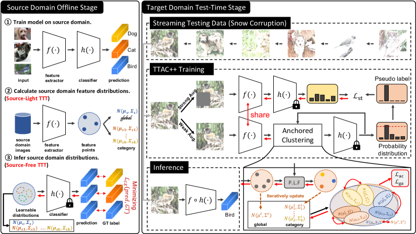
Figure 1: Overview of TTAC++. i) In the source domain offline stage, we calculate or infer category-wise and global distributions in the source domain as anchors. ii) In the test-time stage, testing samples are sequentially streamed and pushed into a fixed-length queue. We apply self-training to testing samples to adapt model weights. Anchored clustering is employed to regularize self-training by aligning source and target domain distributions.

3.1 Anchored Clustering for Test-Time Training

Inspired by the success of discovering cluster structures in the target domain for unsupervised domain adaptation [26], we develop an anchored clustering on the test data alone as the initial module for test-time training. We first use a mixture of Gaussians to model the clusters in the target domain, here each component Gaussian represents one discovered cluster. We further use the distributions of each category in the source domain as anchors for the target distribution to match against. In this way, test data features can simultaneously form clusters and the clusters are associated with source domain categories, resulting in improved generalization to target domain. Formally, we first denote the mixture of Gaussians in the source and target domains as,

$$\begin{split}p_{s}(z)=\sum_{k}\alpha_{k}\mathcal{N}(\mu_{sk},\Sigma_{sk}),\\ p_{t}(z)=\sum_{k}\beta_{k}\mathcal{N}(\mu_{tk},\Sigma_{tk})\end{split}$$ (1)

where $\{\mu_{k}\in\mathbb{R}^{d},\Sigma_{k}\in\mathbb{R}^{d\times d}\}$ represent one cluster in the source/target domain and $d$ is the dimension of feature embedding. Both $\mu_{sk}$ and $\Sigma_{sk}$ can be readily estimated from $\mathcal{D}_{s}$ through MLE. Anchored clustering can be achieved by matching the above two distributions and one may directly minimize the KL-Divergence between the two distribution. Nevertheless, this is non-trivial because the KL-Divergence between two mixture of Gaussians has no closed-form solution which prohibits efficient gradient-based optimization. Despite some approximations exist [49], without knowing the semantic labels for each Gaussian component, even a good match between two mixture of Gaussians does not guarantee target clusters are aligned to the correct source ones and this will severely harm the performance of test-time training. In light of these challenges, we propose a category-wise alignment. Specifically, we allocate the same number of clusters in both source and target domains, each corresponding to one semantic class, and each target cluster is assigned to one source cluster. We can then minimize the KL-Divergence between each pair of clusters as in Eq. 2.

The KL-Divergence can be further decomposed into the entropy $H(\mathcal{N}(\mu_{sk},\Sigma_{sk}))$ and cross-entropy $H(\mathcal{N}(\mu_{sk},\Sigma_{sk}),\mathcal{N}(\mu_{tk},\Sigma_{tk}))$. It is commonly true that the source reference distribution $p_{s}(z)$ is fixed thus the entropy term is a constant $C$ and only the cross-entropy term is to be optimized. Given the closed-form solution to the KL-Divergence between two Gaussian distributions, we now write the anchored clustering objective as,

The source cluster parameters, mean and covariance, can be readily estimated in an offline manner by running through the training samples. These information will not cause any privacy leakage and only introduces a small computation and storage overheads. Nevertheless, one might encounter a more constrained scenario where distributional information on the source domain is prohibited, e.g. downstream user can only have access to model architecture and weights. In the following section, we shall introduce a strict source-free anchored clustering method by inferring source domain clusters. To differentiate the settings, we refer to the former one as source-light TTT, where statistical information on source domain is still available, and the latter one as source-free TTT, where no information on source domain is available.

3.2 Clustering through Pseudo Labeling

In order to test-time train network with anchored clustering loss, one must obtain target cluster parameters $\{\mu_{tk},\Sigma_{tk}\}$. For a minibatch of target test samples $\mathcal{B}^{t}=\{x_{i}\}_{i=tN_{B}\dots(t+1)N_{B}}$ at timestamp $t$, the pseudo labels are obtained via $\hat{y}_{i}=\arg\max_{k}q_{ik}^{t}$. Given the predicted pseudo labels we could estimate the mean and covariance for each component Gaussian with the pseudo labeled testing samples. However, pseudo labels are always subject to model’s discrimination ability. The error rate for pseudo labels is often high when the domain shift between source and target is large, directly updating the component Gaussian is subject to erroneous pseudo labels, a.k.a. confirmation bias [50]. To reduce the impact of incorrect pseudo labels, we first adopt a light-weight temporal consistency (TC) pseudo label filtering approach. Compared to co-teaching [51] or meta-learning [52] based methods, this light-weight method does not introduce additional computation overhead and is therefore more suitable for test-time training. Specifically, to alleviate the impact from the noisy predictions, we calculate the temporal exponential moving averaging posteriors $\tilde{q}^{t}\in[0,1]^{N\times K}$ as below,

$$\tilde{q}^{t}_{i}=(1-\xi)*\tilde{q}^{t-1}_{i}+\xi*q^{t}_{i},\quad s.t.\quad\tilde{q}^{0}_{i}=q^{0}_{i}$$ (4)

The temporal consistency filtering is realized as in Eq. 5 where $\tau_{TC}$ is a threshold determining the maximally allowed difference in the most probable prediction over time. If the posterior deviate from historical value too much, it will be excluded from target domain clustering.

$$F_{i}^{TC}=\mathbbm{1}((q_{i\hat{y}}^{t}-\tilde{q}^{t-1}_{i\hat{y}})>\tau_{TC}),\;s.t.\;\hat{y}=\arg\max_{k}(q_{ik}^{t})$$ (5)

Due to the sequential inference, test samples without enough historical predictions may still pass the TC filtering. So, we further introduce an additional pseudo label filter directly based on the posterior probability as,

$$F_{i}^{PP}=\mathbbm{1}(\tilde{q}^{t}_{i\hat{k}}>\tau_{PP})$$ (6)

By filtering out potential incorrect pseudo labels, we update the component Gaussian only with the leftover target samples as below.

3.3 Global Feature Alignment

As discussed above, test samples that do not pass the filtering will not contribute to the estimation of target clusters. Hence, anchored clustering may not reach its full potential without the filtered test samples. To exploit all available test samples, we propose to align global target data distribution to the source one. We approximate the global feature distribution of the source data as $\hat{p}_{s}(x)=\mathcal{N}(\mu_{s},\Sigma_{s})$ and the target data as $\hat{p}_{t}(x)=\mathcal{N}(\mu_{t},\Sigma_{t})$. To align two distributions, we again minimize the KL-Divergence as,

$$\mathcal{L}_{ga}=D_{KL}(\hat{p}_{s}(x)||\hat{p}_{t}(x))$$ (8)

Similar idea has appeared in [16] which directly matches the moments between source and target domains [34] by minimizing the F-norm for the mean and covariance, i.e. $||\mu_{t}-\mu_{s}||^{2}_{2}+||\Sigma_{t}-\Sigma_{s}||^{2}_{F}$. However, designed for matching complex distributions represented as drawn samples, central moment discrepancy [34] requires summing infinite central moment discrepancies and the ratios between different order moments are hard to estimate. For matching two parameterized Gaussian distributions KL-Divergence is more convenient with good explanation from a probabilistic point of view. Finally, we add a small constant to the diagonal of $\Sigma$ for both source and target domains to increase the condition number for better numerical stability.

3.4 Source-Free TTT by Inferring Source Domain Distributions

In order to enable test-time training under strict source-free setting, we propose to infer the necessary source domain statistical information, i.e. the class-wise mean and covariance matrix, from network weights only. W.o.l.g., we write the classifier head as a linear classifier $h({z}_{i};{w})={w}^{\top}{z}_{i}$ by omitting the bias term, which though can still be preserved in a homogeneous coordinate. Without knowing the true class-wise distribution, we hypothesize that each class $k$ is subject to a uni-modal Gaussian distribution $p_{sk}(z)=\mathcal{N}({\mu}_{sk},{\Sigma}_{sk})$ as given in the previous section. Given a model well trained on the source domain we could expect the following class-wise risk being minimized w.r.t. classifier weights.

$$\begin{split}\mathcal{L}_{sk}({w},{\Theta})=&\mathbbm{E}_{z\sim p_{sk}(z)}[-\log\delta({w}_{k}^{\top}z)]\\ =&\mathbbm{E}_{\tilde{z}\sim\mathcal{N}({0},{I})}[-\log\delta({w}_{k}^{\top}(\mu_{sk}+{A}_{sk}\tilde{z}))]\end{split}$$ (9)

where ${A}_{sk}{A}_{sk}^{\top}={\Sigma}_{sk}$ satisfies a Cholesky decomposition. When source domain feature distribution is unknown while the classifier head ${w}$ is available, we could rewrite the above optimization by substituting the optimization variables to source domain class-wise distribution as below, where the lower bound is derived according to Jensen inequality, as $-\log\delta(\cdot)$ is a convex function. The equality holds when ${A}_{sk}={0}$.

$$\hat{\mathcal{L}}_{sk}(\mu_{sk},{A}_{sk})= \mathbbm{E}_{\tilde{z}\sim\mathcal{N}({0},{I})}[-\log\delta({w}_{k}^{\top}(\mu_{sk}+{A}_{sk}\tilde{z}))]$$ (10)

$$\geq -\log\delta(\mathbbm{E}_{\tilde{z}\sim\mathcal{N}({0},{I})}[{w}_{k}^{\top}(\mu_{sk}+{A}_{sk}\tilde{z})])$$ (11)

$$= -\log\delta({w}_{k}^{\top}{\mu}_{sk})$$ (12)

We interpret this problem as discovering the source domain class-wise distribution such that samples drawn from these distributions can be correctly classified. We argue that directly optimizing Eq. 10 without any constraint on ${A}_{sk}$ is equivalent to optimizing the lower bound, Eq. 12. Because any non-zero ${A}_{sk}$ enables the inequality and without constraining ${A}_{sk}$, a trivial solution with ${A}_{sk}={0}$ exists. Alternatively, one could fix the covariance matrix, ${\Sigma}_{sk}$, and only update class-wise mean, ${\mu}_{sk}$, and this requires Monte Carlo sampling from a standard multi-variate Gaussian distribution should Eq. 10 be the objective to optimize. To get rid of the excessive computation of sampling, we empirically figure out an efficient way to infer source-domain distributions by fixing ${\Sigma}_{sk}=\gamma{I}$ and optimizing the lower bound, Eq. 12, to estimate ${\mu}_{sk}$. Moreover, since all backbone features $z_{i}$ are positive due to ReLu activation, $\mu$ should be all positive so that it may overlap with the true distribution of source domain features. For this purpose, we parameterize $\mu=\hat{\mu}^{2}$ where $\hat{\mu}$ is unconstrained, and add weight decay to $\hat{\mu}$ to limit the norm of $\mu$.

The global feature distribution is approximated by a uni-modal Gaussian distribution. Therefore, to infer the global feature distribution, we use a single Gaussian distribution $\mathcal{N}(\mu_{s},\Sigma_{s})$ to approximate the mixture of per-category Gaussians. Specifically, the following KL-Divergence is minimized with a closed-form solution [49].

3.5 Efficient Iterative Updating

Despite the distribution for source data can be trivially estimated from all available training data in a totally offline manner, estimating the distribution for target domain data is not equally trivial, in particular under the sTTT protocol. In a related research [16], a dynamic queue of test data features are preserved to dynamically estimate the statistics, which will introduce additional memory footprint [16]. To alleviate the memory cost we propose to iteratively update the running statistics for Gaussian distribution. Denoting the running mean and covariance at time stamp $t$ as $\mu^{t}$ and $\Sigma^{t}$, we present the rules to update the mean and covariance in Eq. 14. More detailed derivations and update rules for per cluster statistics are deferred to the Supplementary.

Since $N^{t}$ grows larger overtime, new test samples will have smaller contribution to the update of target domain statistics when $N^{t}$ is large enough. As a result, the gradient calculated from current minibatch will vanish. To alleviate this issue, we impose a clip on the value of $\alpha^{t}$ as below. As such, the gradient can maintain a minimal scale even if $N^{t}$ is very large.

$$a^{t}=\left\{\begin{array}[]{lcl}\frac{1}{N^{t}}&&N^{t}<N_{clip}\\ \frac{1}{N_{clip}}&&others\end{array}\right.$$ (15)

3.6 Self-Training for TTT

Self-training (ST) has been widely adopted in semi-supervised learning where predictions on unlabeled data are admitted as pseudo labels, and model is trained with the pseudo labels [44, 28]. In this work, we explore employing self-training for TTT. Blindly taking all pseudo labels for training has been demonstrated to deteriorate the performance as incorrect pseudo labels act as noisy labels and a high percentage of noisy label is harmful for model training. This phenomenon is also referred to as confirmation bias [50]. As demonstrated in the empirical evaluations in Sect. 4.3, self-training alone is not guaranteed to outperform competing methods. The performance may even degrades after observing enough testing samples as shown in Fig. 4. To reduce the impact of confirmation bias, we first propose to employ anchored clustering as regularization. As anchored clustering allows better alignment between source and target feature distributions, self-training is able to benefit from more accurate pseudo labels and the model is less likely to be harmed by the wrong pseudo labels. This can be achieved by simultaneously optimizing anchored clustering losses and self-training loss. In addition, we further take an approach similar to [28] by filtering out less confident pseudo labels for self-training as in Eq. 16.

where $q(\cdot)=\sigma(h(f(\cdot)))$ denotes the probabilistic posterior, $\hat{y}_{i}=\arg\max_{k}(q(\mathcal{W}(x_{i})))$ denotes the predicted pseudo label, $\mathcal{W}(\cdot)$ denotes a weak augmentation operation consisting of RandomHorizontalFlip and RandomResizedCrop, $\mathcal{A}(\cdot)$ denotes a strong augmentation operation implemented as RandAugment [53], and $\tau_{cr}$ denotes the confidence threshold.

3.7 TTAC++ Training Algorithm

We summarize the training algorithm for the TTAC++ in Algo. 1. For effective clustering in target domain, we allocate a fixed length memory space, denoted as testing time queue $\mathcal{C}\in\mathcal{R}^{N_{C}\times H\times W\times\texttt{3}}$, to store the recent testing samples. In the sTTT protocol, we first make instant prediction on each testing sample, and only update the model when $N_{B}$ testing samples are accumulated. TTAC++ can be efficiently implemented, e.g. with two devices, one is for continuous inference and another is for model updating.

input : A new testing sample batch $\mathcal{B}^{t}=\{x_{i}\}_{i=tN_{B}\dots(t+1)N_{B}}$.

# Update the testing sample queue $\mathcal{C}$.

$\mathcal{C}^{t}=\mathcal{C}^{t-1}\setminus\mathcal{B}^{t-N_{C}/N_{B}}$, $\mathcal{C}^{t}=\mathcal{C}^{t}\bigcup\mathcal{B}^{t}$

for $1$ to $N_{itr}$ do

       for minibatch $\{x^{t}_{i}\}^{N}_{i=1}$ in $\mathcal{C}^{t}$ do

             # Generate weak and strong augmented samples

            $\mathcal{W}(x^{t}_{i}),\quad\mathcal{A}(x^{t}_{i})$

            # Obtain the predicted posterior and pseudo labels

            $q(\mathcal{W}(x_{i}^{t}))=\sigma(h(f(\mathcal{W}(x_{i}^{t}))))$

            $\hat{y}_{i}=\arg\max_{k}(q(\mathcal{W}(x_{i}^{t})))$

            # Update the global and per-cluster running mean and covariance by Eq. 14 with $\mathcal{W}({x_{i}^{t}})$

            $\mu^{t}$, $\Sigma^{t}$, $\{\mu_{k}^{t}\}$, $\{\Sigma_{k}^{t}\}$

            # Calculate the anchored clustering losses according to Eq. 3 and Eq. 8

            $\mathcal{L}_{ac}+\lambda_{1}\mathcal{L}_{ga}$

            # Calculate self-training loss according to Eq. 16

            $\mathcal{L}_{st}$

            # One step gradient descent on the total loss

            $\mathcal{L}_{ac}+\lambda_{1}\mathcal{L}_{ga}+\lambda_{2}\mathcal{L}_{st}$

      

Algorithm 1 TTAC++ Algorithm

4 Experiment

In the experiment section, we first compare against existing methods on different test-time training protocols based on the two key factors. We then ablate the effectiveness of each component in TTAC++. Further analysis on the cumulative performance, qualitative insights, etc. are provided at the end of this section.

4.1 Datasets

We evaluate on five test-time training datasets and report the classification error rate ($\%$) throughout the experiment section. To evaluate the test-time training efficacy on corrupted target images, we use CIFAR10-C/CIFAR100-C [54], each consisting of 10/100 classes with 50,000 training samples of clean data and 10,000 corrupted test samples. We further evaluate test-time training on hard target domain samples with CIFAR10.1 [55], which contains around 2,000 difficult testing images sampled over years of research on the original CIFAR-10 dataset. To demonstrate the ability to do test-time training for synthetic data to real data transfer we further use VisDA-C [56], which is a challenging large-scale synthetic-to-real object classification dataset, consisting of 12 classes, 152,397 synthetic training images and 55,388 real testing images. To evaluate large-scale test-time training, we use ImageNet-C [54] which consists of 1,000 classes and 15 types of corruptions on the 50,000 testing samples. Some qualitative examples of common corruptions on ImageNet-C are illustrated in Fig. 2. Finally, we also evaluate the effectiveness of test-time training against adversarial attacks by implementing TTT on generated adversarial samples on CIFAR-10 dataset, which is referred to as CIFAR-10-adv throughout this work.

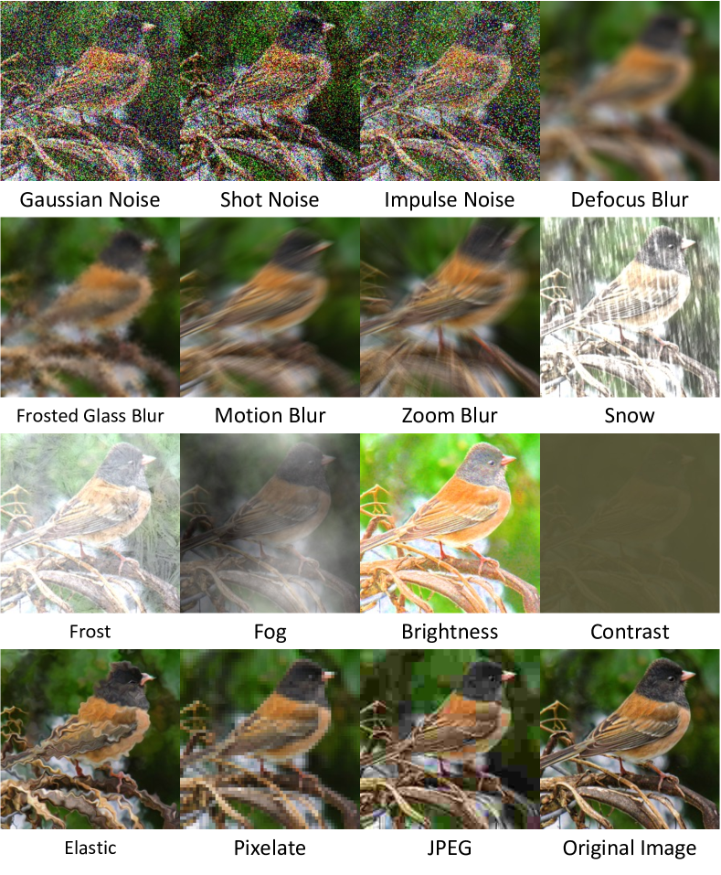
Figure 2: Illustration of corruptions on target domain images. Examples are selected from the ImageNet-C dataset.

4.2 Experiment Settings

4.2.1 Hyperparameters

We use the ResNet-50 [57] as backbone network for fair comparison with existing methods. In addition, ViT [58] was adopted as backbone for evaluation on the compatibility with transformer architectures. We train the backbone network $f(\cdot)$ by SGD optimizer with momentum on all datasets. On CIFAR10-C/CIFAR100-C and CIFAR10.1, we set the batchsize to 256 and the learning rate to 0.01, 0.0001 and 0.01 respectively. On VisDA-C we set the batchsize to 128 and the learning rate to 0.0001. Hyperparameters are shared across multiple TTT protocols except for $N_{C}$ and $N_{itr}$ which are only applicable under one-pass adaptation protocols. $\alpha_{k}$ and $\beta_{k}$ respectively represent the prevalence of each category, here we set them to 1 over the number of categories. $N_{C}$ indicates the length of the testing sample queue $C$ under the sTTT protocol, and $N_{itr}$ controls the update epochs on this queue. $\tau_{TC}$ and $\tau_{PP}$ are the thresholds used for pseudo label filtering. $N_{clip}$ and $N_{clip\_k}$ are the upper bounds of sample counts in the iterative updating of global statistics and target cluster statistics respectively. Finally $\lambda_{1}$ and $\lambda_{2}$ are the coefficients of $\mathcal{L}_{ga}$ and $\mathcal{L}_{cr}$ respectively, which are 1 and 10 respectively. The details of each individual hyperparamter are found in Table. I. When source domain distribution information is not available, we estimate source domain distributions by minimizing Eq. 10 with RMSprop optimizer, learning rate 0.001 and weight decay 0.001. We choose $\gamma=max(svdvals(\Sigma_{\mu sk}))/30.$ for the fixed covariance matrix. Wall-Clock times for competing methods are recorded under PyTorch 1.10.2 framework, CUDA 11.3 and a single NVIDIA RTX 3090 GPU.

TABLE I: Hyper-parameters used on different datasets.

Dataset	$\alpha_{k}$	$\beta_{k}$	$N_{C}$	$N_{itr}$	$\xi$	$\tau_{TC}$	$\tau_{PP}$	$\tau_{cr}$	$N_{clip}$	$N_{clip\_k}$	$\lambda_{1}$	$\lambda_{2}$
CIFAR10-C	0.1	0.1	4096	4	0.9	0.95	-0.001	0.9	1280	128	1.0	10.0
CIFAR100-C	0.01	0.01	4096	4	0.9	0.95	-0.001	0.9	1280	64	1.0	10.0
CIFAR10.1	0.1	0.1	4096	4	0.9	0.95	-0.001	0.9	1280	128	1.0	10.0
VisDA-C	$\frac{1}{12}$	$\frac{1}{12}$	4096	4	0.9	0.95	-0.01	0.9	1536	128	1.0	10.0
ImageNet-C	0.001	0.001	4096	2	0.9	0.95	-0.01	0.9	1280	64	1.0	10.0

4.2.2 Test-Time Training Protocols

We categorize test-time training protocols based on two key factors. First, whether the training objective must be changed during training on the source domain, we use Y and N to indicate if training objective is allowed to be changed or not respectively. Second, whether testing data is sequentially streamed and predicted, we use O to indicate a sequential One-pass inference and M to indicate non-sequential inference, a.k.a. Multi-pass inference. With the above criteria, we summarize 4 test-time training protocols, namely N-O, Y-O, N-M and Y-M, and the strength of the assumption increases from the first to the last protocols. Ours sTTT setting makes the weakest assumption, i.e. N-O. Existing methods are categorized by the four TTT protocols, we notice that some methods can operate under multiple protocols.

Source-Free Test-Time Training. The proposed TTAC++ relies on aligning the source and target domain distributions. It is often realistic to assume having access to the source domain data distributions, which are light-weight and there is no risk of privacy leakage. Nevertheless, for a fair comparison with existing methods that are strictly source-free, we adopt inferring the source domain statistics from source domain model weights only as introduced in Section 3.4. Therefore, we differentiate the source-free (SF) approach from the source-light (SL) approach in the TTT evaluation protocol. We summarize all protocols evaluated in this work in Table. II.

TABLE II: The used components under different TTT protocols.

Protocol	Source Domain Statistics	Contrastive Branch	Multiple Passes
N-O-SF	-	-	-
N-O-SL	✓	-	-
Y-O-SL	✓	✓	-
N-M-SF	-	-	✓
N-M-SL	✓	-	✓
Y-M-SL	✓	✓	✓

TABLE III: Comparison under different TTT protocols. Y/N indicates modifying source domain training objective or not. O/M indicate one pass or multiple passes test-time training. SF/SL indicate source-free and source-light respectively. C10-C, C100-C and C10.1 refer to CIFAR10-C, CIFAR100-C and CIFAR10.1 datasets respectively. All numbers indicate error rate in percentage ($\%$).

Method	TTT Protocol	Assum. Strength	C10-C	C100-C	C10.1
TEST	-	-	29.15	60.34	12.10
BN [59]	N-O-SF	Weak	15.49	43.38	14.00
TENT [20]	N-O-SF	Weak	14.27	40.72	14.40
T3A [21]	N-O-SF	Weak	15.44	42.72	13.50
SHOT [12]	N-O-SF	Weak	13.95	39.10	13.70
Conjugate PL [60]	N-O-SF	Weak	13.21	39.39	14.20
Self-Training [28]	N-O-SF	Weak	14.66	39.25	12.85
TTAC++ (Ours)	N-O-SF	Weak	11.62	37.76	12.85
TTT++ [16]	N-O-SL	Weak	13.69	40.32	13.65
TTAC [61]	N-O-SL	Weak	10.94	36.64	12.80
TTAC+SHOT [61]	N-O-SL	Weak	10.99	36.39	12.40
TTAC++ (Ours)	N-O-SL	Weak	9.78	35.48	12.20
TTT++ [16]	Y-O-SL	Medium	13.00	35.23	12.60
TTAC [61]	Y-O-SL	Medium	10.69	34.82	12.00
TTAC++ (Ours)	Y-O-SL	Medium	10.05	34.30	11.55
BN [59]	N-M-SF	Medium	15.70	43.30	14.10
TENT [20]	N-M-SF	Medium	12.60	36.30	13.65
SHOT [12]	N-M-SF	Medium	14.70	38.10	14.25
TTAC++ (Ours)	N-M-SF	Medium	9.14	34.43	10.60
TTT++ [16]	N-M-SL	Medium	11.87	37.09	11.95
TTAC [61]	N-M-SL	Medium	9.42	33.55	11.00
TTAC+SHOT [61]	N-M-SL	Medium	9.54	32.89	11.30
TTAC++ (Ours)	N-M-SL	Medium	7.23	29.23	9.00
TTT-R [19]	Y-M-SL	Strong	14.30	40.40	11.00
TTT++ [16]	Y-M-SL	Strong	9.80	34.10	9.50
TTAC [61]	Y-M-SL	Strong	8.52	30.57	9.20
TTAC++ (Ours)	Y-M-SL	Strong	7.57	29.08	8.90

TABLE IV: Test-time training on ImageNet-C under the sTTT (N-O) protocol.

Method	Brit	Contr	Defoc	Elast	Fog	Frost	Gauss	Glass	Impul	Jpeg	Motn	Pixel	Shot	Snow	Zoom	Avg
TEST	38.82	89.55	82.23	87.13	64.84	76.83	97.34	90.50	97.76	68.31	83.60	80.37	96.74	82.22	74.31	80.70
BN (N-O-SF)	32.33	50.93	81.28	52.98	42.21	64.13	83.25	83.64	82.52	59.18	66.23	49.45	82.59	62.34	52.51	63.04
TENT (N-O-SF)	31.39	40.27	75.68	42.03	35.38	64.32	84.92	84.96	81.43	46.84	49.48	39.77	84.21	49.23	43.49	56.89
SHOT (N-O-SF)	30.69	37.69	61.97	41.30	34.74	54.19	76.33	71.94	74.24	46.50	47.98	38.88	70.60	46.09	40.74	51.59
Conjugate PL (N-O-SF)	30.62	34.28	61.12	40.40	34.43	51.80	65.61	67.75	63.71	44.61	45.70	38.41	63.07	45.83	41.27	48.57
Self-Training (N-O-SF)	31.57	37.62	79.68	42.84	35.27	54.18	88.76	91.93	81.22	51.97	50.29	39.73	88.67	48.52	47.07	57.95
TTAC++ (N-O-SF)	31.61	36.55	60.39	38.79	34.20	49.02	61.62	62.67	59.37	45.25	44.73	38.43	58.32	43.60	39.99	46.97
TTAC (N-O-SL)	30.36	38.84	69.06	39.67	36.01	50.20	66.18	70.17	64.36	45.59	51.77	39.72	62.43	44.56	42.80	50.11
TTAC++ (N-O-SL)	29.78	34.37	58.08	37.68	32.97	47.96	60.51	62.24	58.65	43.61	43.58	36.89	57.33	42.40	38.82	45.66

4.2.3 Competing Methods

We compare the following test-time training methods. Direct testing (TEST) without adaptation simply do inference on target domain with source domain model. Test-time training (TTT-R) [19] jointly trains the rotation-based self-supervised task and the classification task in the source domain, and then only train the rotation-based self-supervised task in the streaming test samples and make the predictions instantly. The default method is classified into the Y-M protocol. Test-time normalization (BN) [59] moving average updates the batch normalization statistics by streamed data. The default method follows N-M protocol and can be adapted to N-O protocol. Test-time entropy minimization (TENT) [20] updates the parameters of all batch normalization by minimizing the entropy of the model predictions in the streaming data. By default, TENT follows the N-O protocol and can be adapted to N-M protocol. Test-time classifier adjustment (T3A) [21] computes target prototype representation for each category using streamed data and make predictions with updated prototypes. T3A follows the N-O protocol by default. Source Hypothesis Transfer (SHOT) [12] freezes the linear classification head and trains the target-specific feature extraction module by exploiting balanced category assumption and self-supervised pseudo-labeling in the target domain. SHOT by default follows the N-M protocol and we adapt it to N-O protocol. TTT++ [16] aligns source domain feature distribution, whose statistics are calculated offline, and target domain feature distribution by minimizing the F-norm between the mean covariance. TTT++ follows the Y-M protocol and we adapt it to N-O (removing contrastive learning branch) and Y-O protocols. AdaContrast [22] approaches TTT from a self-training perspective. Pseudo labels on target domain testing samples are generated from a weak augmentation branch and used for supervising a strong augmentation branch. Conjugate PL [39] proposed to learn the best TTT objective through meta-learning. This approach discovered a loss similar to the entropy loss adopted by Tent when source domain is trained with cross-entropy loss. Self-Training [28], a.k.a. FixMatch, was originally developed for semi-supervised learning by estimating pseudo labels on the unlabeled data and supervise model training with pseudo labels. We adapt FixMatch to TTT by adopting the self-training component alone and refer to it as Self-Training (ST). TTAC [61] aligns the source and target domain feature distributions for TTT. It requires a single pass on the target domain and does not have to modify the source training objective. TTAC was originally implemented for all TTT protocols. TTAC was further augmented with additional diversity loss and entropy minimization loss introduced in SHOT [12], denoted as TTAC+SHOT [61]. Finally, we evaluate our proposed method, TTAC++, under all TTT protocols. For Y-O and Y-M protocols we incorporate an additional contrastive learning branch introduced in [16].

4.3 Test-Time Training Evaluations

We evaluate test-time training on four types of target domain data, including images with corruptions, manually selected hard images, synthetic to real adaptation and adversarial samples.

4.3.1 TTT on Corrupted Target Domain

We present the test-time training results on CIFAR10/100-C datasets in Tab. III, and the results on ImageNet-C dataset in Tab. IV. For ImageNet-C, we only evaluate under the realistic sTTT (N-O) protocol. We make the following observations from the results.

sTTT (N-O) Protocol. We first analyze the results under the proposed sTTT (N-O) protocol. Our method outperforms all competing ones by a large margin both with source domain statistics (N-O-SL) and without source domain statistics (N-O-SF). Under the most strict N-O-SF protocol, TTAC++ leads the benchmark with a large margin. It outperforms Conjugate PL by $1.6\%$ on CIFAR10-C and SHOT by $1.4\%$ on CIFAR100-C. When source domain statistics are available, TTAC++ gains additional advantage. Compared with TTT++, we achieved $4\%$ and $5\%$ improvements on CIFAR10-C and CIFAR100-C datasets respectively. TTAC++ also improves upon TTAC+SHOT where the latter adopts a class balance assumption. On ImageNet-C dataset, TTAC++ demonstrates its superiority under both N-O-SF and N-O-SL protocols. Without source domain statistics, TTAC++ outperforms Conjugate PL on 11 out of 15 types of corruptions. When source domain statitics are available, TTAC++ consistently outperforms TTAC with similar data augmentation.

TABLE V: Test-time training on the VisDA-C dataset.

Method	Protocol	Plane	Bcycl	Bus	Car	Horse	Knife	Mcycl	Person	Plant	Sktbrd	Train	Truck	Avg
-	TEST	56.52	88.71	62.77	30.56	81.88	99.03	17.53	95.85	51.66	77.86	20.44	99.51	65.19
N-O-SF	TENT	19.75	81.99	17.78	40.03	21.64	19.04	11.66	38.18	23.15	77.33	35.88	98.31	40.40
	SHOT	10.81	18.62	27.08	59.65	11.13	56.43	27.29	26.22	13.76	47.35	22.26	61.18	31.82
	Self-Training	4.69	21.12	13.67	16.00	4.03	89.64	6.19	86.35	3.17	88.82	15.18	98.05	37.24
	TTAC++	11.63	22.42	18.49	33.47	9.57	18.89	10.28	21.92	10.75	24.46	18.51	90.37	24.23
N-O-SL	TTAC	18.54	40.20	35.84	63.11	23.83	39.61	15.51	41.35	22.97	46.56	25.24	67.81	36.71
	TTAC++	7.13	31.34	21.79	43.07	7.57	13.25	7.52	27.95	8.33	32.00	14.16	63.66	23.15
Y-O-SL	TTAC	7.19	29.99	22.52	56.58	8.14	18.41	8.25	22.28	10.18	23.98	13.55	67.02	24.01
	TTAC++	4.85	26.45	20.98	44.01	5.41	7.47	6.90	21.95	6.53	27.49	12.58	68.91	21.13
N-M-SF	BN	44.38	56.98	33.24	55.28	37.45	66.60	16.55	59.02	43.55	60.72	31.07	82.98	48.99
	TENT	13.43	77.98	20.17	48.15	21.72	82.45	12.37	35.78	21.06	76.41	34.11	98.93	45.21
	SHOT	5.73	13.64	23.33	42.69	7.93	86.99	19.17	19.97	11.63	11.09	15.06	43.26	25.04
	Self-Training	4.44	26.91	16.25	22.87	3.45	60.53	5.59	53.50	4.31	61.25	17.68	95.04	30.99
	AdaContrast	4.28	14.65	22.52	27.58	4.24	7.23	13.77	13.00	6.05	87.46	9.28	51.98	21.84
	TTAC++	7.62	17.93	15.69	27.17	5.27	9.73	7.32	21.28	7.19	21.35	15.18	92.93	20.72
N-M-SL	TTT++	28.25	32.03	33.67	64.77	20.49	56.63	22.52	36.30	24.84	35.20	25.31	64.24	37.02
	TTAC	14.43	36.52	34.90	61.94	21.34	45.06	13.41	39.12	17.48	42.83	25.24	65.36	34.80
	TTAC++	5.46	27.02	18.14	38.19	5.69	11.47	7.18	28.77	7.50	13.28	13.17	59.82	19.64
Y-M-SL	TTT++	4.13	26.20	21.60	31.70	7.43	83.30	7.83	21.10	7.03	7.73	6.91	51.40	23.03
	TTAC	2.74	17.73	18.91	43.12	5.54	12.24	4.66	15.90	4.77	10.78	9.75	62.45	17.38
	TTAC++	2.61	16.86	16.82	38.41	4.28	2.89	4.93	18.20	4.29	6.27	8.78	62.76	15.59

Alternative Protocols. We further compare different methods under N-M, Y-O and Y-M protocols. Under the Y-O protocol, TTT++ [16] modifies the source domain training objective by incorporating a contrastive learning branch [62]. To compare with TTT++, we also include the contrastive branch and observe a clear improvement on both CIFAR10-C and CIFAR100-C datasets. Other TTT methods are adapted to the N-M protocol by allowing training on the whole target domain data multiple epochs. Specifically, we compared with BN, TENT and SHOT. With TTAC alone we observe substantial improvement on all three datasets and TTAC can be further combined with SHOT demonstrating additional improvement. Finally, under the Y-M protocol, we demonstrate very strong performance compared to TTT-R and TTT++. It is also worth noting that TTAC under the N-O protocol can already yield results close to TTT++ under the Y-M protocol, suggesting the strong test-time training ability of TTAC even under the most challenging TTT protocol.

4.3.2 TTT on Selected Hard Samples as Target Domain

CIFAR10.1 contains roughly 2,000 new test images that were re-sampled after the research on original CIFAR-10 dataset, which consists of some hard samples and reflects the normal domain shift in our life. Evaluation of TTT methods on CIFAR10.1 is widely adopted to verify the benefit of adapting to hard target domain samples. We present the results on CIFAR10.1 in Table. III. Again, we observe a strong performance of TTAC++ under all TTT protocols.

4.3.3 TTT on Synthetic Source to Real Target Domains

VisDA-C is a large-scale benchmark of synthetic-to-real object classification dataset. We demonstrate on this dataset the ability of TTT to adapt model trained on synthetic source domain to realistic target domain data. On this dataset, we conduct experiments under the N-O, Y-O, N-M and Y-M protocols with results presented in Table. V. We make the following observations from the results. First, our proposed method, TTAC++, outperforms all competing methods under all evaluation protocols. In particular, the improvement for TTAC++ is very significant under the N-O (sTTT) protocol regardless of access to source domain statistics. For example, TTAC++ outperforms the previous best method, the SHOT, by $7\%$ under N-O-SF and, the TTAC, by $13\%$ under N-O-SL. Moreover, TTAC++ also demonstrates very competitive performance when multiple passes on the target domain is allowed (N-M-SF), a.k.a. source-free domain adaptation.

4.3.4 TTT on Adversarial Target Domain

The existing test-time training/adaptation works often evaluate adaptation to the target domain with hand-crafted corruptions. In this section, we investigate the robustness of test-time training subject to stronger out-of-distribution data, i.e. adversarial samples.

This evaluation reveals that simple test-time training can substantially improve model’s robustness to adversarial testing samples. In specific, we generate adversarial samples on the testing set of CIFAR-10 dataset by $L^{\infty}$ PGD [63] attack with $\epsilon=8/255$, 40 iterations and attack step size $0.01$. The adversarial testing samples are then frozen for TTT evaluation. We extensively evaluated existing TTT methods and present the results in Tab. VI. We make the following observations from the results. First, without any test-time adaptation, direct testing with source domain model yields very poor performance ($93.07\%$). This is consistent with previous investigations into adversarial attacks. Furthermore, existing test-time training methods which do not consider self-training, e.g. BN, TENT and SHOT, performs relatively poor compared with methods equipped with self-training, e.g. Self-Training, TTT++ and TTAC++. We attribute the performance gap to the fact that the data augmentation applied during self-training is able to smooth out the adversarial noise. Self-training is able to exploit the pseudo labels predicted on smoothed testing samples and improve the accuracy. Finally, we observe that distribution matching is complementary to purely self-training, suggested by the improvement of TTAC++ from Self-Training under N-O-SF and N-M-SF protocols. Overall, we demonstrate that TTAC++ is a strong test-time training paradigm, it owns the ability to adapt to adversarial corruption which is stronger than hand-crafted natural corruptions.

TABLE VI: Evaluations on test-time training for adversarial samples of CIFAR10 dataset. Each number in the table indicates error rate in percentage.

Protocol	Method	Airpl.	Automob.	Bird	Cat	Deer	Dog	Frog	Horse	Ship	Truck	Avg
-	TEST	97.00	84.90	95.20	93.20	95.70	96.30	95.00	95.70	88.80	88.90	93.07
N-O-SF	BN	95.80	62.30	89.50	90.60	91.70	79.60	78.10	73.60	83.10	67.20	81.15
	TENT	96.70	65.60	92.10	92.80	93.20	86.40	82.40	78.70	90.50	73.00	85.14
	SHOT	97.50	50.60	90.80	93.50	93.90	74.30	78.00	67.60	85.00	65.50	79.67
	Self-Training	43.10	12.20	48.20	53.00	45.30	45.90	48.40	42.30	29.20	35.00	40.26
	TTAC++	36.70	14.70	45.80	60.70	37.80	40.70	23.40	33.30	25.60	27.60	34.63
N-O-SL	TTT++	89.60	46.60	79.90	86.00	83.80	66.40	60.80	47.90	72.70	56.10	68.98
	TTAC	60.20	26.30	58.60	68.20	62.10	47.10	41.40	29.70	36.90	37.20	46.77
	TTAC++	23.90	12.60	32.00	53.50	34.60	33.90	20.20	15.90	17.20	18.80	26.26
Y-O-SL	TTT++	37.80	15.00	47.70	58.50	41.80	38.60	26.10	20.20	19.00	21.90	32.66
	TTAC	32.40	14.50	42.60	58.80	42.10	37.50	23.20	18.70	16.00	23.00	30.88
	TTAC++	23.30	11.20	32.30	54.10	31.70	30.90	17.80	15.10	14.70	18.60	24.97
N-M-SF	BN	96.20	59.10	87.90	90.90	90.70	79.80	74.80	72.30	82.90	64.70	79.93
	TENT	96.00	66.60	91.50	92.20	93.90	83.20	81.20	76.90	87.10	71.50	84.01
	SHOT	96.70	48.10	89.50	93.50	93.00	75.30	78.60	43.40	80.60	64.70	76.34
	Self-Training	30.70	4.40	35.90	54.30	39.10	18.50	45.80	30.30	19.90	26.90	30.58
	TTAC++	23.10	8.10	36.60	36.90	29.50	41.20	16.90	50.30	26.50	20.30	28.94
N-M-SL	TTT++	74.90	28.50	68.00	78.30	71.40	51.70	47.70	31.10	52.70	40.90	54.52
	TTAC	36.60	15.10	46.30	54.40	47.60	39.10	28.90	21.90	21.30	22.10	33.33
	TTAC++	11.10	5.60	15.40	28.90	14.50	17.40	9.30	7.00	6.20	10.10	12.55
Y-M-SL	TTT++	19.30	6.80	30.10	41.90	25.60	27.50	14.20	10.60	7.80	11.60	19.54
	TTAC	18.50	6.90	31.40	43.20	29.00	32.00	16.50	11.70	6.90	12.20	20.83
	TTAC++	11.20	3.90	15.70	26.50	14.50	17.10	7.60	7.40	5.60	9.50	11.90

4.3.5 TTT Cumulative Performance

A good test-time training framework should benefit from seeing more testing samples and the performance on the target domain is expected to be gradually increasing. In this section, we compare different test-time training methods by illustrating the cumulative error rate on CIFAR10/100-C and ImageNet-C (Gaussian Blur corruption) under the sTTT protocols (N-O-SF/SL) in Fig. 3 and Fig. 4, respectively. As we observe from the figure, some existing TTT methods do not benefit from seeing more testing samples. For example, BN and T3A’s performance stabilize after 2000 testing samples on CIFAR10/100-C. The performance of TENT and Self-Training (ST) even degrade after observing 10000 to 20000 testing samples on ImageNet-C. This empirical evaluation also suggest applying self-training alone for TTT is prone to confirmation bias and may harm the performance. In contrast, TTAC++ (pink solid line) exhibits the fastest drop of error rate among all source-free methods. Compared with all methods requiring access to source domain statistics or changing source domain training objectives, TTAC++ is is consistently lower in error rate along the TTT procedure. More importantly, the trend (sharp slope) shows higher potential for TTAC++ should more testing samples are available in the target domain.

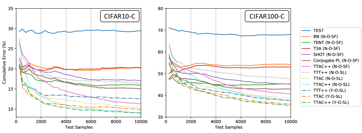
Figure 3: Test-time cumulative error rate on CIFAR10/100-C datasets.

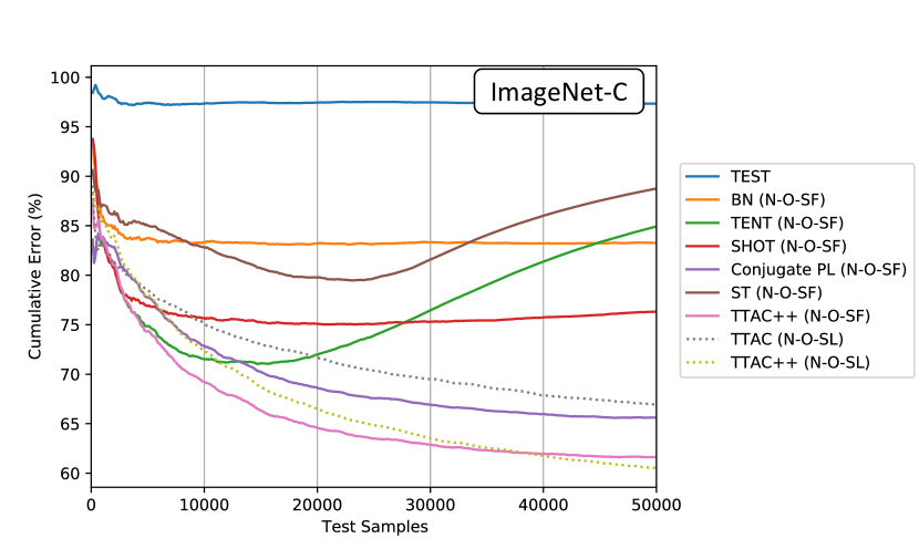
Figure 4: Test-time cumulative error on ImageNet-C dataset with Gaussian Blur corruption.

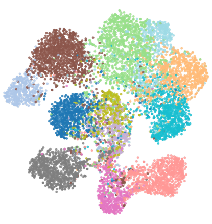
(a) TTAC Feature

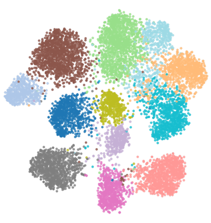
(b) TTAC++ Feature

Figure 5: To reduce the computation, we select 10,000 samples on VisDA-C dataset to draw the T-SNE visualizations. (a) T-SNE visualization of TTAC feature embedding. (b) T-SNE visualization of TTAC++ feature embedding.

4.3.6 TSNE Visualization of TTAC++ features

We provide qualitative results for test-time training by visualizing the adapted features through T-SNE [64]. In Fig. 5 (a) and Fig. 5 (b), we compare the features learned by TTAC [61] and TTAC++. We observe a better separation between classes by TTAC++, implying an improved classification accuracy.

4.4 Ablation Study

In this section, we validate the effectiveness of individual components, including anchored clustering, pseudo label filtering, global feature alignment, self-training and finally the compatibility with contrastive branch [16], on CIFAR10-C dataset. For anchored clustering alone, we use all testing samples to update cluster statistics. For pseudo label filtering alone, we implement as predicting pseudo labels followed by filtering, then pseudo labels are used for self-training. We make the following observations from Tab. VII. Under both N-O and N-M protocols, introducing anchored clustering or pseudo label filtering alone improves over the baseline, e.g. under N-O $29.15\%\rightarrow 14.32\%$ for anchored clustering and $29.15\%\rightarrow 15.00\%$ for pseudo label filtering. When anchored clustering is combined with pseudo label filtering, we observe a significant boost in performance. This is due to more accurate estimation of category-wise cluster in the target domain. We further evaluate aligning global features alone with KL-Divergence. This achieves relatively good performance and obviously outperforms the L2 distance alignment adopted in [16]. Next, when self-training is turned on in conjunction with other components, we observe a consistent improvement under all TTT protocols. Finally, we combine all components with additional contrastive branch and the full model yields the best performance under both Y-O-SL and Y-M-SL protocols.

TABLE VII: Ablation study for individual components on CIFAR10-C dataset.

TTT Protocol		N-O-SL						Y-O-SL		N-M-SL						Y-M-SL
Anchored Cluster.	-	✓	-	✓	-	✓	✓	✓	✓	✓	✓	-	-	✓	✓	✓	✓
Pseudo Label Filter.	-	-	✓	✓	-	✓	✓	✓	✓	-	✓	-	-	✓	✓	✓	✓
Global Feat. Align.	-	-	-	-	KLD	KLD	KLD	KLD	KLD	-	-	L2 Dist.[16]	KLD	KLD	KLD	KLD	KLD
Self-Training	-	-	-	-	-	-	✓	-	✓	-	-	-	-	-	✓	-	✓
Contrast. Branch [16]	-	-	-	-	-	-	-	✓	✓	-	-	-	-	-	-	✓	✓
Avg Acc	29.15	14.32	15.00	11.33	11.72	10.94	9.78	10.69	10.05	11.11	10.01	11.87	10.8	9.42	7.23	8.52	7.57

4.5 Additional Analysis

In this section, we provide additional investigations into additional the designs that affect computation efficiency, compatibility with additional backbones, randomness, and alternative designs, etc.

TABLE VIII: Evaluating compatibility with ViT backbone on CIFAR10-C dataset.

Method	Brit	Contr	Defoc	Elast	Fog	Frost	Gauss	Glass	Impul	Jpeg	Motn	Pixel	Shot	Snow	Zoom	Avg	Std
TEST	2.29	16.24	4.83	9.45	13.60	6.73	24.52	18.23	24.48	12.63	7.63	14.57	23.02	5.29	3.50	12.47	7.36
BN	2.29	16.24	4.83	9.45	13.60	6.73	24.52	18.23	24.48	12.63	7.63	14.57	23.02	5.29	3.50	12.47	7.36
TENT	1.84	3.55	3.31	7.01	5.57	4.09	60.97	10.20	61.12	9.72	4.93	3.87	22.47	4.55	2.64	13.72	19.19
SHOT	2.00	3.13	3.46	6.63	5.79	4.06	11.65	9.39	10.58	9.69	5.03	3.63	10.05	4.35	2.70	6.14	3.15
TTT++	1.91	4.14	3.88	6.58	6.27	4.00	10.08	8.59	8.85	9.66	4.68	3.62	9.17	4.28	2.74	5.90	2.64
TTAC	2.15	4.05	3.91	6.62	5.67	3.75	9.26	7.95	7.97	8.55	4.75	3.87	8.24	3.93	2.94	5.57	2.24
TTAC++	1.59	3.01	3.70	6.19	4.45	3.25	9.14	7.76	8.02	7.84	4.14	3.64	7.80	3.38	2.47	5.09	2.36

4.5.1 Test Sample Queue and Update Epochs.

Under the sTTT protocol, we allow all competing methods to maintain the same test sample queue and multiple update epochs on the queue. To analyze the significance of the sample queue and update epochs, we evaluate BN, TENT, SHOT, TTAC and TTAC++ on CIFAR10-C and ImageNet-C level 5 snow corruption evaluation set under different number of update epochs on test sample queue and under a without queue protocol, i.e. only update model w.r.t. the current test sample batch. As the results presented in Tab. IX, we make the following observations. i) Maintaining a sample queue can substantially improve the performance of methods that estimate target distribution, e.g. TTAC++ ($11.18\rightarrow 10.31$), TTAC ($11.91\rightarrow 10.88$ on CIFAR10-C) and SHOT ($15.18\rightarrow 13.96$ on CIFAR10-C). This is due to more test samples giving a better estimation of true distribution. ii) Consistent improvement can be observed with increasing update epochs for SHOT, TTAC and TTAC++. We ascribe this to iterative pseudo labeling benefiting from more update epochs. These observations also provide insights for deploying TTT for real-world practice. By considering memory constraint and demand for real-time model update, one can adjust the queue length and number of update epochs to strike a balance between efficiency and performance.

TABLE IX: Comparing with and without test sample queue and different numbers of model update epochs. w/ Queue maintains a test sample queue with 4096 samples; w/o Queue maintains a single mini-batch with 256 and 128 samples on CIFAR10-C and ImageNet-C respectively.

	CIFAR10-C					ImageNet-C
	w/ Queue				w/o Queue	w/ Queue		w/o Queue
#Epochs	1	2	3	4*	1	1	2*	1
BN	15.84	15.99	16.04	16.00	15.44	62.34	62.34	62.59
TENT	13.35	13.83	13.85	13.87	13.48	47.82	49.23	48.39
SHOT	13.96	13.93	13.83	13.75	15.18	46.91	46.09	51.46
TTAC	10.88	10.80	10.58	10.01	11.91	45.44	44.56	46.64
TTAC++	10.31	9.40	9.08	8.82	11.18	43.49	42.40	46.01

TABLE X: The per-sample wall time (measured in seconds) on CIFAR10-C under sTTT protocol.

	w/ Queue				w/o Queue
#Epochs	1	2	3	4	1
BN	0.0136	0.0220	0.0293	0.0362	0.0030
TENT	0.0269	0.0399	0.0537	0.0663	0.0041
SHOT	0.0479	0.0709	0.0942	0.1183	0.0067
TTAC	0.0516	0.0822	0.1233	0.1524	0.0083
TTAC++	0.0706	0.1076	0.1591	0.1963	0.0090
Inference	0.0030	0.0030	0.0030	0.0030	0.0030

TABLE XI: The performance of TTAC under different data streaming orders.

Random Seed	0	10	20	200	300	3000	4000	40000	50000	500000	Avg
Error ($\%$)	8.82	8.80	9.38	9.13	8.88	8.87	9.07	8.93	9.02	8.68	8.96$\pm$0.19

TABLE XII: Comparison of alternative strategies for updating target domain clusters.

Strategy	Brit	Contr	Defoc	Elast	Fog	Frost	Gauss	Glass	Impul	Jpeg	Motn	Pixel	Shot	Snow	Zoom	Avg
i. Without filtering	6.01	7.21	8.13	13.87	9.03	9.82	13.13	18.22	15.66	11.47	9.26	9.29	11.68	9.19	6.79	10.58
ii. Soft Assignment	5.91	6.52	8.05	13.25	9.08	9.76	13.14	17.19	15.45	11.41	8.88	9.10	11.53	9.13	6.83	10.35
Filtering (Ours)	5.59	6.28	7.53	12.99	8.95	9.22	12.13	15.79	14.37	10.65	8.70	8.60	10.70	8.82	6.37	9.78

4.5.2 Computation Cost Measured in Wall-Clock Time

Test sample queue and multiple update epochs introduce additional computation overhead. To investigate the impact on efficiency, we measure the overall wall time as the time elapsed from the beginning to the end of test-time training, including all I/O overheads. The per-sample wall time is then calculated as the overall wall time divided by the number of test samples. We report the per-sample wall time (in seconds) for BN, TENT, SHOT, TTAC and TTAC++ in Tab. X under different update epoch settings and without queue setting. The Inference row indicates the per-sample wall-clock time in a single forward pass including data I/O overhead. We observe that, under the same experiment setting, BN and TENT are more computational efficient, but TTAC++ is only 2 to 3 times more expensive than BN and TENT if no test sample queue is preserved (0.0090 v.s. 0.0030/0.0041) while the performance of TTAC++ w/o queue is still better than TENT (11.18 v.s. 13.48). In summary, TTAC++ is able to strike a balance between computation efficiency and performance depending on how much computation resource is available. This suggests allocating a separate device for model weights update is only necessary when securing best performance is the priority.

4.5.3 Evaluation of compatibility with Transformer Backbone

In this section, we provide additional evaluation of TTAC++ with a transformer backbone, ViT [58]. In specific, we pre-train ViT on CIFAR10 clean dataset and then follow the sTTT protocol to do test-time training on CIFAR10-C testing set. The results are presented in Tab. VIII. We report the average (Avg) and standard deviation (Std) of accuracy over all 15 categories of corruptions. Again, TTAC++ consistently outperform all competing methods with transformer backbone.

4.5.4 Impact of Data Streaming Order

The proposed sTTT protocols assumes test samples arrive in a stream and inference is made instantly on each test sample. The result for each test sample will not be affected by any following ones. In this section, we investigate how the data streaming order will affect the results. Specifically, we randomly shuffle all testing samples in CIFAR10-C for 10 times with different seeds and calculate the mean and standard deviation of test accuracy under sTTT protocol. The results in Tab. XI suggest TTAC++ maintains consistent performance regardless of data streaming order.

4.5.5 Sensitivity to Hyperparameters

We evaluate the sensitivity to two thresholds during pseudo label filtering, namely the temporal smoothness threshold $\tau_{TC}$ and posterior threshold $\tau_{PP}$. In particular, $\tau_{TC}$ controls how much the maximal probability deviate from the historical exponential moving average (ema). If the current value is lower than the ema below a threshold, we believe the prediction is not confident and the sample should be excluded from estimating target domain cluster. $\tau_{PP}$ controls the the minimal maximal probability and below this threshold is considered as not confident enough. We evaluate $\tau_{TC}$in the interval between 0 and -1.0 and $\tau_{PP}$ in the interval from 0.5 to 0.95 with results on CIFAR10-C level 5 glass blur corruption presented in Tab. XIII. We draw the following conclusions on the evaluations. First, there is a wide range of hyperparameters that give stable performance, e.g. $\tau_{TC}\in[0.5,0.0.9]$ and $\tau_{PP}\in[-0.0001,-0.01]$. Second, when temporal consistency filtering is turn off, i.e. $\tau_{TC}=-1.0$, because the probability is normalized to between 0 and 1, the performance drops substantially, suggesting the necessity to apply temporal consistency filtering.

TABLE XIII: Evaluation of pseudo labeling thresholds on CIFAR10-C level 5 glass blur corruption. Numbers are reported as classification error (%).

$\tau_{TC}\backslash\tau_{PP}$	0.5	0.6	0.7	0.8	0.9	0.95
0.0	23.03	22.26	21.96	22.50	21.14	28.55
-0.0001	20.03	20.53	20.45	20.40	19.49	27.00
-0.001	19.66	20.51	19.49	20.48	19.42	26.83
-0.01	20.71	20.78	20.73	20.65	20.29	27.58
-0.1	24.10	21.47	21.46	22.36	21.45	28.71
-1.0	30.75	24.08	23.40	24.33	22.21	28.77

4.5.6 Alternative Strategies for Updating Target Domain Clusters

In Sect. 3.2, we presented target domain clustering through pseudo labeling. A temporal consistency approach is adopted to filter out confident samples to update target clusters. In this section, we discuss two alternative strategies for updating target domain clusters. Firstly, each target cluster can be updated with all samples assigned with respective pseudo label (without Filtering). This strategy will introduce many noisy samples into cluster updating and potentially harm test-time feature learning. Secondly, we use a soft assignment of testing samples to each target cluster to update target clusters (Soft Assignment). This strategy is equivalent to fitting a mixture of Gaussian through EM algorithm. We compare these two alternative strategies with our temporal consistency based filtering approach. The results are presented in Tab. XII. We find the results with temporal consistency based filtering outperforms the other two strategies on 13 out of 15 categories of corruptions, suggesting pseudo label filtering is necessary for estimating more accurate target clusters.

4.5.7 Alternative Design for Inferring Source Domain Distributions

In this work, we develop a solution to infer the source distributions in Sect. 3.4. Alternative to learning the distribution mean, an alternative solution is developed by re-scaling the classifier weight [65]. In this section, we compare the two options for estimating source domain statistics with results presented in Tab. XIV. We conclude from the comparison that learning source domain statistics (TTAC++) is clearly better than re-scaling classifier weights [65]. We attribute the advantage of TTAC++ to the fact that backbone features are obtained after ReLu activation, thus being all positive. The classifier weights are trained without any constraints and could have negative weights. The mismatch between classifier weights and backbone features might lead to inferior results by using re-scaled classifier weights as source domain distribution mean.

TABLE XIV: Comparing alternative methods to estimate source domain distributions.

Method	Error (%)
Class. Weights [65]	13.79
TTAC++ (SF)	11.62

4.5.8 Limitations and Failure Cases

Finally, we discuss the limitations of TTAC++ from two perspectives. First, we point out that TTAC++ requires backpropagation to update models at testing stage, therefore additional computation overhead is required. As shown in Tab. X, TTAC++ is 2-5 times computationally more expensive than BN and TENT. However, contrary to usual expectation, BN and TENT are also very expensive compared with no adaptation at all. Eventually, most test-time training methods might require an additional device for test-time adaptation.

We further discuss the limitations on test-time training under more severe corruptions. Specifically, we evaluate TENT, SHOT, TTAC, and TTAC++ under 1-5 levels of corruptions on CIFAR10-C with results reported in Tab. XV. We observe generally a drop of performance from 1-5 level of corruption. Despite consistently outperforming TENT and SHOT at all levels of corruptions, TTAC++’s performance at higher corruption levels are relatively worse, suggesting future attention must be paid to more severely corrupted scenarios.

TABLE XV: Classification error under different levels of snow corruption on CIFAR10-C dataset.

Level	1	2	3	4	5
TEST	9.46	18.34	16.89	19.31	21.93
TENT	8.76	11.39	13.37	15.18	13.93
SHOT	8.70	11.21	13.16	15.12	13.76
TTAC	6.54	8.19	9.82	10.61	10.01
TTAC++	6.05	7.83	8.47	9.43	8.82

5 Conclusion

Test-time training (TTT) tackles the realistic challenges of deploying domain adaptation on-the-fly. In this work, we are first motivated by the confused evaluation protocols for TTT and proposed two key criteria, namely modifying source training objective and sequential inference, to further categorize existing methods into four TTT protocols. Under the most realistic protocol, i.e. sequential test-time training (sTTT), we developed a test-time anchored clustering (TTAC) approach to align target domain features to the source ones. Unlike batchnorm and classifier prototype updates, anchored clustering allows all network parameters to be trainable, thus demonstrating stronger test-time training ability. We further proposed pseudo label filtering and an iterative update method to improve anchored clustering and save memory footprint respectively. When source domain distribution information is absent, we proposed to infer the distribution for anchored clustering through efficient gradient based optimization to achieve source-free sTTT. Finally, we incorporated self-training to update model weights with high confidence pseudo labels. We demonstrated self-training is particularly helpful with anchored clustering as regularization, and the improved model is referred to as TTAC++. Experiments on five datasets verified the effectiveness of TTAC++ under sTTT as well as other TTT protocols. We hope this work will serve as an in time taxonomy of TTT protocols and future works can be compared fairly under respective protocols.

Acknowledgement: This work was supported in part by the National Natural Science Foundation of China (NSFC) under Grant 62106078, Guangdong R&D key project of China (No.: 2019B010155001), the Program for Guangdong Introducing Innovative and Enterpreneurial Teams (No.: 2017ZT07X183), and A*STAR Career Development Award (Grant no. C210112059).

Yongyi Su received the B.E. degree from South China University of Technology in 2021. He is currently working toward the PhD degree in the School of Electronic and Information Engineering, South China University of Technology, Guangzhou, China. His research interests mainly include 3D weakly supervised learning, domain adaptation, test-time training and robust learning.

Xun Xu received the B.E. degree from Sichuan University, in 2010 and the PhD degree from Queen Mary University of London in 2016. He was a research fellow with National University of Singapore between 2016 and 2019. He is now with I2R, A*STAR. His research interests include semi-supervised learning, domain adaptation, zero-shot learning with applications to 3D point cloud data.

Tianrui Li (SM’11) received the B.S., M.S., and Ph.D. degrees from Southwest Jiaotong University, Chengdu, China, in 1992, 1995, and 2002, respectively. He was a Post-Doctoral Researcher with Belgian Nuclear Research Centre, Mol, Belgium, from 2005 to 2006, and a Visiting Professor with Hasselt University, Hasselt, Belgium, in 2008; University of Technology, Sydney, Australia, in 2009; and University of Regina, Regina, Canada, in 2014. He is currently a Professor and the Director of the Key Laboratory of Cloud Computing and Intelligent Techniques, Southwest Jiaotong University. He has authored or co-authored over 300 research papers in refereed journals and conferences. His research interests include big data, machine learning, data mining, granular computing, and rough sets.

Kui Jia received the B.E. degree from Northwestern Polytechnic University, Xi’an, China, in 2001, the M.E. degree from the National University of Singapore, Singapore, in 2004, and the Ph.D. degree in computer science from the Queen Mary University of London, London, U.K., in 2007. He was with the Shenzhen Institute of Advanced Technology of the Chinese Academy of Sciences, Shenzhen, China, Chinese University of Hong Kong, Hong Kong, the Institute of Advanced Studies, University of Illinois at Urbana-Champaign, Champaign, IL, USA, and the University of Macau, Macau, China. He is currently a Professor with the School of Electronic and Information Engineering, South China University of Technology, Guangzhou, China. His recent research focuses on theoretical deep learning and its applications in vision and robotic problems, including deep learning of 3D data and deep transfer learning.

References

- [1] A. Krizhevsky, I. Sutskever, and G. E. Hinton, “Imagenet classification with deep convolutional neural networks,” in Advances in neural information processing systems, 2012.
- [2] J. Carreira and A. Zisserman, “Quo vadis, action recognition? a new model and the kinetics dataset,” in proceedings of the IEEE Conference on Computer Vision and Pattern Recognition, 2017.
- [3] Z.-H. Zhou, “A brief introduction to weakly supervised learning,” National science review, 2018.
- [4] J. Quiñonero-Candela, M. Sugiyama, A. Schwaighofer, and N. D. Lawrence, Dataset shift in machine learning. Mit Press, 2008.
- [5] S. Ben-David, J. Blitzer, K. Crammer, A. Kulesza, F. Pereira, and J. W. Vaughan, “A theory of learning from different domains,” Machine learning, 2010.
- [6] S. J. Pan and Q. Yang, “A survey on transfer learning,” IEEE Transactions on knowledge and data engineering, 2009.
- [7] M. Wang and W. Deng, “Deep visual domain adaptation: A survey,” Neurocomputing, 2018.
- [8] Y. Ganin and V. Lempitsky, “Unsupervised domain adaptation by backpropagation,” in International conference on machine learning, 2015.
- [9] E. Tzeng, J. Hoffman, K. Saenko, and T. Darrell, “Adversarial discriminative domain adaptation,” in Proceedings of the IEEE conference on computer vision and pattern recognition, 2017.
- [10] J. Hoffman, E. Tzeng, T. Park, J.-Y. Zhu, P. Isola, K. Saenko, A. Efros, and T. Darrell, “Cycada: Cycle-consistent adversarial domain adaptation,” in International conference on machine learning, 2018.
- [11] K. Zhou, Z. Liu, Y. Qiao, T. Xiang, and C. Change Loy, “Domain generalization: A survey,” IEEE Transactions on Pattern Analysis and Machine Intelligence, 2022.
- [12] J. Liang, D. Hu, and J. Feng, “Do we really need to access the source data? Source hypothesis transfer for unsupervised domain adaptation,” in International Conference on Machine Learning, 2020.
- [13] J. N. Kundu, N. Venkat, R. V. Babu et al., “Universal source-free domain adaptation,” in Proceedings of the IEEE/CVF Conference on Computer Vision and Pattern Recognition, 2020.
- [14] S. Yang, Y. Wang, J. van de Weijer, L. Herranz, and S. Jui, “Generalized source-free domain adaptation,” in Proceedings of the IEEE/CVF International Conference on Computer Vision, 2021.
- [15] H. Xia, H. Zhao, and Z. Ding, “Adaptive adversarial network for source-free domain adaptation,” in Proceedings of the IEEE/CVF International Conference on Computer Vision, 2021.
- [16] Y. Liu, P. Kothari, B. van Delft, B. Bellot-Gurlet, T. Mordan, and A. Alahi, “Ttt++: When does self-supervised test-time training fail or thrive?” in Advances in Neural Information Processing Systems, 2021.
- [17] Z. Qiu, Y. Zhang, H. Lin, S. Niu, Y. Liu, Q. Du, and M. Tan, “Source-free domain adaptation via avatar prototype generation and adaptation,” in International Joint Conference on Artificial Intelligence, 2021.
- [18] J. Huang, D. Guan, A. Xiao, and S. Lu, “Model adaptation: Historical contrastive learning for unsupervised domain adaptation without source data,” in Advances in Neural Information Processing Systems, 2021.
- [19] Y. Sun, X. Wang, Z. Liu, J. Miller, A. Efros, and M. Hardt, “Test-time training with self-supervision for generalization under distribution shifts,” in International Conference on Machine Learning, 2020.
- [20] D. Wang, E. Shelhamer, S. Liu, B. Olshausen, and T. Darrell, “Tent: Fully test-time adaptation by entropy minimization,” in International Conference on Learning Representations, 2021.
- [21] Y. Iwasawa and Y. Matsuo, “Test-time classifier adjustment module for model-agnostic domain generalization,” in Advances in Neural Information Processing Systems, 2021.
- [22] D. Chen, D. Wang, T. Darrell, and S. Ebrahimi, “Contrastive test-time adaptation,” in Proceedings of the IEEE/CVF Conference on Computer Vision and Pattern Recognition, 2022.
- [23] Y. Gandelsman, Y. Sun, X. Chen, and A. A. Efros, “Test-time training with masked autoencoders,” in Advances in Neural Information Processing Systems, 2022.
- [24] A. C. Gilbert, Y. Zhang, K. Lee, Y. Zhang, and H. Lee, “Towards understanding the invertibility of convolutional neural networks,” in Proceedings of the 26th International Joint Conference on Artificial Intelligence, 2017.
- [25] Q. Li, Z. Wen, Z. Wu, S. Hu, N. Wang, Y. Li, X. Liu, and B. He, “A survey on federated learning systems: vision, hype and reality for data privacy and protection,” IEEE Transactions on Knowledge and Data Engineering, 2021.
- [26] H. Tang, K. Chen, and K. Jia, “Unsupervised domain adaptation via structurally regularized deep clustering,” in Proceedings of the IEEE/CVF conference on computer vision and pattern recognition, 2020.
- [27] D.-H. Lee et al., “Pseudo-label: The simple and efficient semi-supervised learning method for deep neural networks,” in Workshop on challenges in representation learning, ICML, 2013.
- [28] K. Sohn, D. Berthelot, N. Carlini, Z. Zhang, H. Zhang, C. A. Raffel, E. D. Cubuk, A. Kurakin, and C.-L. Li, “Fixmatch: Simplifying semi-supervised learning with consistency and confidence,” Advances in neural information processing systems, 2020.
- [29] H. Liu, J. Wang, and M. Long, “Cycle self-training for domain adaptation,” in Advances in Neural Information Processing Systems, 2021.
- [30] E. Tzeng, J. Hoffman, N. Zhang, K. Saenko, and T. Darrell, “Deep domain confusion: Maximizing for domain invariance,” arXiv preprint arXiv:1412.3474, 2014.
- [31] M. Long, Y. Cao, J. Wang, and M. Jordan, “Learning transferable features with deep adaptation networks,” in International conference on machine learning, 2015.
- [32] A. Gretton, K. M. Borgwardt, M. J. Rasch, B. Schölkopf, and A. Smola, “A kernel two-sample test,” Journal of Machine Learning Research, 2012.
- [33] B. Sun and K. Saenko, “Deep coral: Correlation alignment for deep domain adaptation,” in European conference on computer vision, 2016.
- [34] W. Zellinger, T. Grubinger, E. Lughofer, T. Natschläger, and S. Saminger-Platz, “Central moment discrepancy (cmd) for domain-invariant representation learning,” in International Conference on Learning Representations, 2016.
- [35] J. Jiang and C. Zhai, “Instance weighting for domain adaptation in nlp,” in ACL, 2007.
- [36] H. Yan, Y. Ding, P. Li, Q. Wang, Y. Xu, and W. Zuo, “Mind the class weight bias: Weighted maximum mean discrepancy for unsupervised domain adaptation,” in Proceedings of the IEEE conference on computer vision and pattern recognition, 2017.
- [37] J. Liang, D. Hu, Y. Wang, R. He, and J. Feng, “Source data-absent unsupervised domain adaptation through hypothesis transfer and labeling transfer,” IEEE Transactions on Pattern Analysis and Machine Intelligence, 2021.
- [38] Q. Wang, O. Fink, L. Van Gool, and D. Dai, “Continual test-time domain adaptation,” in Proceedings of the IEEE/CVF International Conference on Computer Vision, 2022.
- [39] S. Goyal, M. Sun, A. Raghunathan, and J. Z. Kolter, “Test time adaptation via conjugate pseudo-labels,” in Advances in Neural Information Processing Systems, 2022.
- [40] M. Choi, J. Choi, S. Baik, T. H. Kim, and K. M. Lee, “Test-time adaptation for video frame interpolation via meta-learning,” IEEE Transactions on Pattern Analysis and Machine Intelligence, 2021.
- [41] J. E. Van Engelen and H. H. Hoos, “A survey on semi-supervised learning,” Machine Learning, 2020.
- [42] X. Zhu, Z. Ghahramani, and J. D. Lafferty, “Semi-supervised learning using gaussian fields and harmonic functions,” in Proceedings of the International conference on Machine learning, 2003.
- [43] A. Iscen, G. Tolias, Y. Avrithis, and O. Chum, “Label propagation for deep semi-supervised learning,” in Proceedings of the IEEE/CVF Conference on Computer Vision and Pattern Recognition, 2019.
- [44] D. Berthelot, N. Carlini, I. Goodfellow, N. Papernot, A. Oliver, and C. A. Raffel, “Mixmatch: A holistic approach to semi-supervised learning,” Advances in neural information processing systems, 2019.
- [45] A. Kumar, T. Ma, and P. Liang, “Understanding self-training for gradual domain adaptation,” in International Conference on Machine Learning, 2020.
- [46] X. Xu, J. Liao, L. Cai, M. C. Nguyen, K. Lu, W. Zhang, Y. Yazici, and C. S. Foo, “Revisiting pretraining for semi-supervised learning in the low-label regime,” arXiv preprint arXiv:2205.03001, 2022.
- [47] D. Wang, S. Liu, S. Ebrahimi, E. Shelhamer, and T. Darrell, “On-target adaptation,” arXiv preprint arXiv:2109.01087, 2021.
- [48] S. Sinha, P. Gehler, F. Locatello, and B. Schiele, “Test: Test-time self-training under distribution shift,” in Proceedings of the IEEE/CVF Winter Conference on Applications of Computer Vision, 2022.
- [49] J. R. Hershey and P. A. Olsen, “Approximating the kullback leibler divergence between gaussian mixture models,” in IEEE International Conference on Acoustics, Speech and Signal Processing, 2007.
- [50] E. Arazo, D. Ortego, P. Albert, N. E. O’Connor, and K. McGuinness, “Pseudo-labeling and confirmation bias in deep semi-supervised learning,” in International Joint Conference on Neural Networks, 2020.
- [51] B. Han, Q. Yao, X. Yu, G. Niu, M. Xu, W. Hu, I. Tsang, and M. Sugiyama, “Co-teaching: Robust training of deep neural networks with extremely noisy labels,” in Advances in neural information processing systems, 2018.
- [52] J. Li, Y. Wong, Q. Zhao, and M. S. Kankanhalli, “Learning to learn from noisy labeled data,” in Proceedings of the IEEE/CVF Conference on Computer Vision and Pattern Recognition, 2019.
- [53] E. D. Cubuk, B. Zoph, J. Shlens, and Q. V. Le, “Randaugment: Practical automated data augmentation with a reduced search space,” arXiv preprint arXiv:1909.13719, 2019.
- [54] D. Hendrycks and T. Dietterich, “Benchmarking neural network robustness to common corruptions and perturbations,” in International Conference on Learning Representations, 2019.
- [55] B. Recht, R. Roelofs, L. Schmidt, and V. Shankar, “Do imagenet classifiers generalize to imagenet?” in International Conference on Machine Learning, 2019.
- [56] X. Peng, B. Usman, N. Kaushik, J. Hoffman, D. Wang, and K. Saenko, “Visda: The visual domain adaptation challenge,” arXiv preprint arXiv:1710.06924, 2017.
- [57] K. He, X. Zhang, S. Ren, and J. Sun, “Deep residual learning for image recognition,” in Proceedings of the IEEE conference on computer vision and pattern recognition, 2016.
- [58] A. Dosovitskiy, L. Beyer, A. Kolesnikov, D. Weissenborn, X. Zhai, T. Unterthiner, M. Dehghani, M. Minderer, G. Heigold, S. Gelly, J. Uszkoreit, and N. Houlsby, “An image is worth 16x16 words: Transformers for image recognition at scale,” in International Conference on Learning Representations, 2021.
- [59] S. Ioffe and C. Szegedy, “Batch normalization: Accelerating deep network training by reducing internal covariate shift,” in International conference on machine learning, 2015.
- [60] S. Goyal, M. Sun, A. Raghunathan, and Z. Kolter, “Test-time adaptation via conjugate pseudo-labels,” in Advances in Neural Information Processing Systems, 2022.
- [61] Y. Su, X. Xu, and K. Jia, “Revisiting realistic test-time training: Sequential inference and adaptation by anchored clustering,” in Advances in Neural Information Processing Systems, 2022.
- [62] T. Chen, S. Kornblith, M. Norouzi, and G. Hinton, “A simple framework for contrastive learning of visual representations,” in International conference on machine learning, 2020.
- [63] A. Madry, A. Makelov, L. Schmidt, D. Tsipras, and A. Vladu, “Towards deep learning models resistant to adversarial attacks,” in International Conference on Learning Representations, 2018.
- [64] L. Van der Maaten and G. Hinton, “Visualizing data using t-sne.” Journal of machine learning research, 2008.
- [65] N. Ding, Y. Xu, Y. Tang, C. Xu, Y. Wang, and D. Tao, “Source-free domain adaptation via distribution estimation,” in Proceedings of the IEEE/CVF Conference on Computer Vision and Pattern Recognition, 2022, pp. 7212–7222.