Each state in a one-dimensional disordered system has two localization lengths when the Hilbert space is constrained

Abstract

In disordered systems, the amplitudes of the localized states will decrease exponentially away from their centers and the localization lengths are characterizing such decreasing. In this article, we find a model in which each eigenstate is decreasing at two distinct rates. The model is a one-dimensional disordered system with a constrained Hilbert space: all eigenstates $|\Psi\rangle$s should be orthogonal to a state $|\Phi\rangle$, $\langle\Phi|\Psi\rangle=0$, where $|\Phi\rangle$ is a given exponentially localized state. Although the dimension of the Hilbert space is only reduced by $1$, the amplitude of each state will decrease at one rate near its center and at another rate in the rest region, as shown in Fig. 1. Depending on $|\Phi\rangle$, it is also possible that all states are changed from localized states to extended states. In such a case, the level spacing distribution is different from that of the three well-known ensembles of the random matrices. This indicates that a new ensemble of random matrices exists in this model. Finally we discuss the physics behind such phenomena and propose an experiment to observe them.

I Introductions

In Anderson localization, every localized state is characterized by one quantity called the localization length $\lambda$. It describes how much the state is localized in the real space, $|\Psi_{E}({\vec{r}})|\sim e^{-|\vec{r}-\vec{r}_{0}|/\lambda(E)}$Evers and Mirlin (2008), where $r_{0}$ is the center of the state at which the wavefunction takes the maximum value and $E$ is the eigenenergy. This ansatz still applies thoroughly in the Anderson disordered models in recent works, from one-dimension(1D) to three dimensionDe Tomasi et al. (2016); Lin and Popović (2015); Wang et al. (2015); Belitz and Kirkpatrick (2016), from the localized states to the extended states with $\lambda=0$Yusipov et al. (2017); Xiong and Xiong (2007); Sheinfux et al. (2017); Pasek et al. (2017); Delande et al. (2017); Di Sante et al. (2017); Tikhonov et al. (2016); García-Mata et al. (2017); Smith et al. (2017); Murphy et al. (2017); Huckestein (1995); Lee and Fisher (1981) and from Gaussian orthogonal ensemble (GOE) to Gaussian symplectic ensemble (GSE) of random matricesBeenakker (1997); Brody et al. (1981).

But in this article, we find that this ansatz may be broken down when an extra constraint is subjected to the Hilbert space, $\langle\Phi|\Psi\rangle=0$. In another word, the dimension of the effective Hilbert space spanned by $|\Psi\rangle$s is reduced by $1$ because $|\Phi\rangle$ is not in such Hilbert space. Erasing a site at $i$ from a lattice is an example of such a constraint. Here $|\Phi\rangle=|i\rangle$ and the effective Hilbert space is on the rest lattice. In this article, the $|\Phi\rangle$ we are considering is an exponentially decreasing function, which is neither the eigenstate of the Hamiltonian nor the eigenstate of the position operator. We study the eigenstates of a 1D disordered lattice in such constrained Hilbert space(CHS) and find that each state needs two localization lengths to characterize its localization. As Fig. 1(b) shown, the states first exponentially decrease faster near their centers and then their decreasing change to a slower rate. When $\alpha=0$, as shown in Fig. 1(c), all states become extended, regardless of how strong the disorder is in such 1D system.

The article is organized as follows: we first write down the static Schrödinger equation for a 1D disordered lattice in CHS. Interestingly, such an equation is changed from homogeneous to non-homogeneous. The equation is solved numerically on a finite lattice to show the eigenstates. Then the transfer matrix method is developed to take part in the non-homogeneous term. We argued that the ensemble of the orthogonal states during the QR decomposition should be reexamined to pick up the correct Lyapunov exponents. The distribution of the level spacing is also distinct from that of the traditional disordered systems. Finally, we discuss how to realize such constraint in an experiment.

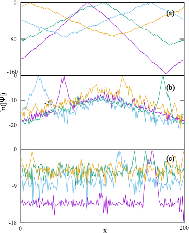
Figure 1: (a) The eigenstates in the real space for the Anderson disordered model. (b) and (c) Those for the model with CHS. For the sake of clarity, only $4$ typical states are plotted and the other states are similar. Each state in (b) has two localization lengths while it is an extended state in (c). The length of the ring is $N=200$, the strength of the disorder is $W=10$ and $\alpha$ is $0.1$ in (b) and $0$ in (c).

II The non-homogeneous Schrödinger equation in CHS

We consider the Hamiltonian for a 1D Anderson disordered lattice with the on-site disorders,

$$H_{D}=\sum_{x=1}^{N}(|x\rangle\langle x+1|+h.c.)+\sum_{x=1}^{N}\epsilon_{x}|x\rangle\langle x|,$$ (1)

where $\epsilon_{x}$ are the random numbers within $[-W/2,W/2]$, $x$ is the index of the site on the 1D lattice and the integer $N$ is the length. We take the periodic boundary condition in the calculations.

It is well-known that the standard static Schrödinger equation $E|\Psi\rangle=H_{D}|\Psi\rangle$ can be obtained by minimizing $\langle\Psi|H_{D}|\Psi\rangle$ under the constraint $\langle\Psi|\Psi\rangle=1$. The eigenenergy $E$ is a Lagrange multiplier. Now as we have one more constraint $\langle\Psi|\Phi\rangle=0$, the static Schrödinger equation changes to

$$E|\Psi\rangle = H_{D}|\Psi\rangle+\mu|\Phi\rangle,$$ (2)

$$\langle\Phi|\Psi\rangle = 0.$$ (3)

Here $\mu$ is another Lagrange multiplier and it should take the value to make $\langle\Phi|\Psi\rangle=0$. In the section on the experimental setup, we will give another argument to prove the validity of the above equations.

The eigenvalues $E$ and the corresponding eigenfunctions $|\Psi\rangle$ can be found by solving a general eigenproblem

$$\begin{pmatrix}EI&0\\ 0&0\end{pmatrix}\begin{pmatrix}|\Psi\rangle\\ \mu\end{pmatrix}=\begin{pmatrix}H_{D}&|\Phi\rangle\\ \langle\Phi|&0\end{pmatrix}\begin{pmatrix}|\Psi\rangle\\ \mu\end{pmatrix},$$ (4)

where $I$ is a $N\times N$ identity matrix. It is also equivalent to an eigenproblem for a defective non-hermitian matrixXiong (2021).

We plot several eigenstates $\Psi(x)=\langle x|\Psi\rangle$ in Fig. 1(b). The strength of disorder is $W=10$ and the wavefunction in the constraint is $\Phi(x)=e^{-\alpha|x-x_{0}|}$ whose center $x_{0}$ is at the center of the ring. We use the GEM package in octave to perform the calculation with much higher precision so that the results have not been smeared out by the round-off errors. For the sake of comparative analysis, we first plot the traditional eigenstates of $H_{D}$ in Fig. 1(a). Every state is decreasing exponentially over the whole chain at a constant rate, $\frac{1}{\xi(E)}$. In Fig. 1(b), the wavefunctions first decrease rapidly around their centers and then change to decrease/increase at a slower rate. After fitting the data, we find this slower rate is $\alpha$, which is independent of the eigenenergies $E$ and the central positions of the wavefunctions. When $\alpha=0$, as shown in Fig. 1(c), all states become extended, regardless of the strength of the disorder.

In traditional 1D disordered models, as the states $\Psi_{0}(x)$s are exponentially localized, the local environments at a far distance should not affect the states. The overlaps with $\Phi(x)$, $\langle\Phi|\Psi_{0}\rangle\sim\max\{e^{-\alpha d},e^{-\frac{1}{\lambda}d}\}$, are exponentially small but are not exactly zero. Here $d$ is the distance between the centers of $\Psi_{0}(x)$ and $\Phi(x)$. To make such overlap be exactly zero, as the constraint requires, the state $\Psi(x)$ must be disturbed from $\Psi_{0}(x)$ in the scale of $\max\{e^{-\alpha d},e^{-\frac{1}{\lambda}d}\}$. This is confirmed in our calculations as the Lagrange multiplier $\mu\sim\max\{e^{-\alpha d},e^{-\frac{1}{\lambda}d}\}$. So an exponentially small factor $\mu$ in the non-homogeneous Schrödinger equation Eq. 2 is important and can affect the character of localization in the far distance. This is distinct from many equations in which an exponentially small term is ignorable. To confirm this conclusion, we employ the transfer matrix method to study the localization lengths of such a system.

III The transfer matrix method in CHS

The traditional transfer matrix method is used to calculate the Lyapunov exponents of the transfer matrix that is relating the wavefunctions on the $L$th and the $(L+1)$th slices with those on the $0$th and the $1$st slicesMacKinnon and Kramer (1981); Pichard and Sarma (1981); MacKinnon and Kramer (1983) . It is subjected to the homogeneous Schrödinger equation and only the diagonal elements of the $R$ matrix during the $QR$ decomposition are interestedLuo et al. (2021). Here we first extend the method to the non-homogeneous case and argue that the orthogonalized vectors in the $Q$ matrix should be inspected first.

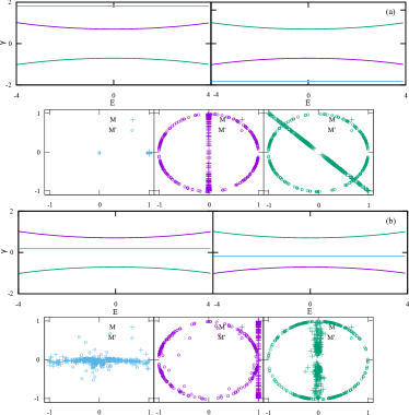
Figure 2: (a) The three Lyapunov exponents, $\alpha$ and $\pm\frac{1}{\lambda(E)}$ ($-\alpha$ and $\mp\frac{1}{\lambda(E)}$) as the function of energy $E$ for the transfer matrix $M$ (left) and $M^{\prime}$ (right). For each Lyapunov exponent $\gamma$ on the left, there is its partner $-\gamma$ on the right. The first two components of the orthonormal columns in $Q$, $\vec{z}_{i}$s, are plotted below for the three pairs of Lyapunov exponents. There are $1000$ disorder configurations being considered and their $\vec{z}_{i}$s are all plotted in the figures. The colors of the points are used to distinguish the corresponding Lyapunov exponent and the “plus” and the “circle” symbols are for $M$ and $M^{\prime}$, respectively. Here $\alpha=1.83>\frac{1}{\lambda(E)}$, $W=10$ and $E=1$. As there is no overlap between $\{\vec{z}_{i}\}$s for the pair $(\alpha,-\alpha)$, $\alpha$ is not the true exponent to describe the asymptotic behaviors of the states. (b) When $\alpha=0.18<\frac{1}{\lambda(E)}$, the overlaps emerge so that both $\alpha$ and $\frac{1}{\lambda(E)}$ are describing the asymptotic behaviors of the states simultaneously.

We redefine the transfer matrix $M_{x}(E)$ as the square matrix in

$$\begin{pmatrix}\Psi_{x+1}\\ \Psi_{x}\\ \Phi_{x+R+1}\end{pmatrix}=\begin{pmatrix}E-\epsilon_{x}&-1&\mu e^{\alpha R}\\ 1&0&0\\ 0&0&e^{-\alpha}\end{pmatrix}\begin{pmatrix}\Psi_{x}\\ \Psi_{x-1}\\ \Phi_{x+R}\end{pmatrix},$$ (5)

where $\Psi_{x}$ is the wavefunctions on the $x$th slice (the $x$th lattice in our 1D model), $E$ is the energy, $\Phi_{x+R}$ is the wavefunction of $|\Phi\rangle$ on the $(x+R)$th site. Here $\Phi$ is offset $R$ sites so that $\mu e^{\alpha R}$ is in the scale of the unit even when $\mu$ is exponentially small. As $\mu$ has been determined by the constraint but the exact value of $\mu$ is not important in this treatment, the constraint is not needed to be written down explicitly in the transfer matrix. In another word, after $\mu$ is determined by the equation of the constraint, we can always choose a proper offset $R$ to scale the term $\mu e^{\alpha R}$.

The transfer matrix $M=\prod_{x=1}^{L}M_{x}$ can be $QR$ decomposed into the product of a matrix $Q$ having orthonormal columns and an upper triangular matrix $R$. The diagonal elements of $R$ matrix are $e^{L\gamma_{i}}$, where $\gamma_{i}$ are the Lyapunov exponents and the orthonormal columns in $Q$, $\vec{z}_{i}$, are the corresponding typical states. Due to the variations of the disordered configurations, each $\vec{z}_{i}$ actually forms a group of ensemble $\{\vec{z}_{i}\}$. If the typical state $\vec{z}_{i}$ does exist for the disordered chain, one must find consistent results regardless of viewing the chain from the left to the right or from the right to the left. So the ensemble of $\{\vec{z}_{i}\}$ for the Lyapunov exponent $\gamma_{i}$ must match or at least overlaps with the ensemble of $\{\vec{z}^{\prime}_{i}\}$ for the Lyapunov exponent $-\gamma_{i}$ of the transfer matrix $M^{\prime}=\prod_{x=L}^{1}M^{\prime}_{x}$. Here the transfer matrix $M^{\prime}$ is counting from $x=L$(the right) to $x=1$ (the left) and $M^{\prime}_{x}$ is the same as $M_{x}$ except that the last element is replaced by $e^{\alpha}$ because the decreasing $\Phi(x)$ changes to the increasing function as reversing $x$.

The three Lyapunov exponents of the transfer matrix $M$ are $\alpha$ and $\pm\gamma(E)$, where $\pm\gamma(E)$ are the exponents of the disordered chain in the absence of constraint. So it seems that the redefinition of the transfer matrix only enrolls an additional exponent $\alpha$ which can be attributed to the asymptotic behavior of $\Phi(x)$. But as shown in Fig. 2(a), some of the exponents are untrue. We first plot the exponents as the function of the energy $E$ for the transfer matrix $M$ and the transfer matrix $M^{\prime}$, respectively. For each exponent $\gamma_{i}$ for $M$, there is a $-\gamma_{i}$ exponent for $M^{\prime}$. Then the ensemble of the corresponding typical states $\vec{z}_{i}$ for such pairs of exponents are plotted. As these typical states are normalized, only the first two components of the states are plotted. When $\alpha>\frac{1}{\lambda(E)}$, it is shown that the ensembles of $\vec{z}$ and $\vec{z}^{\prime}$ for the pair ($\alpha$, $-\alpha$) do not overlap with each other. So $\frac{1}{\alpha}$ is not the localization length of the model, because if the corresponding typical state in $Q$ matrix does exist, it should be observed independent of viewing from the left or the right. In such case, each state is only characterized by one localization length, $\lambda(E)$. This conclusion is reasonable because in the extreme case $\alpha\to\infty$, $\Phi(x)$ is a delta function so the constraint is equivalent to the elimination of the center site from the lattice. This will only change the ring with $L$ sites to a chain with $L-1$ sites. All bulk localized states are not affected by such boundary condition so the localization behavior of the model is the same as that of a traditional disordered model. But when $\alpha<\gamma(E)$, in Fig. 2(b), the ensembles overlap so that both $\frac{1}{\alpha}$ and $\lambda(E)$ are the localization lengths simultaneously.

IV The distribution of the level spacing

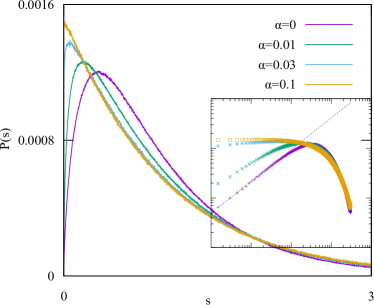
Figure 3: The distributions of the normalized level spacing $s$ for $\alpha=0,0.01,0.03,0.1$, respectively. The inset shows the same distributions in logarithmic axes. The straight line, $f(s)\sim s^{0.64}$, is a guide to the eye. The length of the ring is $N=600$, the strength of disorder is $W=10$ and $10^{7}$ samples are considered in the statistics.

In the 1D Anderson disordered lattice, the distribution of the level spacing is a Poisson curve $\sim e^{-s}$, where $s$ is the normalized nearest neighboring eigenenergy spacing. The maximal distribution appears at $s=0$, which indicates that all eigenstates are localized and cannot repulse the other states in the energy. When the states become extended, such repulsion exercises so that the distribution is changed to the Wigner distributionWigner (1951); Dyson (1962a, b)

$$P(s)\sim s^{\beta}e^{-\frac{\pi\beta^{4}}{4}s^{2}},$$ (6)

where $\beta$ is $1$, $2$ and $4$ for the orthogonal, the unitary and the symplectic ensembles, respectively.

In Fig. 3, we show such distributions $P(s)$ when the constraint is subjected. When $\alpha=0.1$, although the eigenstates are still characterized by two localization lengths, the distribution is still a Poisson function. As $\alpha$ is decreasing, one of the localization lengths becomes longer and longer and dominates the asymptotic behaviors of the states. So they become more and more extended. This is confirmed by the fact that the distribution is distinct from the Poisson function and becomes more and more Wigner-like. When $\alpha=0$, all states should become extended and the distribution becomes a Wigner function exactly. But interestingly, as the inset shows, the $\beta$ of such Wigner function is $0.64$, a value distinct from those of the three well-known ensembles. This indicates that the mechanics to delocalize the states in this model are different from that of the competition between the disordered potential and the kinetic energy. We have no more discussions on the new ensemble at this stage. But we think the emergence of the new ensemble is related to the non-hermitian random matrix at an exceptional point because Eq. 4 is equivalent to the eigenproblem of a non-hermitian defective matrix.

V The experiments to observe the phenomena

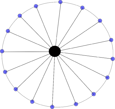
Figure 4: The electron on the quantum dots (blue points) can jump to the nearest-neighboring dots or the central quantum dot (black point). The thin lines indicate the hoppings between the dots.

The CHS can be realized in microscopic electronic systems, macroscopic mechanical systems, or optical systems. We consider a ring of quantum dots (resonant cavities) with effective hoppings between the nearest neighboring dots (cavities). From now on, we will only focus on the system of quantum dots but the mechanics are the same in the other systems. The disorder is introduced by the on-site energies of the dots. There is another dot at the center of the ring. Such a dot is weakly connected with all dots on the ring by an effective hopping $t^{\prime}$. The energy level of the center dot is detuned to be $\delta$ away from the energy $E$ we are considering. After projecting out the level of the center dot, the Hamiltonian for the dots on the ring is

$$H_{\text{LR}}=H_{D}+\sum_{x,x^{\prime}}\frac{t^{\prime 2}}{\delta}|x\rangle\langle x^{\prime}|,$$ (7)

where $H_{D}$ is the disordered Hamiltonian and the later term describes the effective hoppings between any pair of quantum dots mediated by the center dot. Such long-range hopping termSantos et al. (2016); Celardo et al. (2016) can also be written as $\frac{t^{\prime 2}}{\delta}N|\Phi\rangle\langle\Phi|$, where $N$ is the number of dots on the ring and $|\Phi\rangle=\frac{1}{\sqrt{N}}\sum_{x}|x\rangle$. When $\frac{t^{\prime 2}}{\delta}N$ is a huge number as compared to the energy scale of $H_{D}$, the spectrum of $H_{\text{LR}}$ are composed by a band with $N-1$ levels and one level $|\Phi\rangle$ at the huge energy. Because the eigenstates of a hermitian Hamiltonian are orthogonal to each other, the states in the band, $|\Psi\rangle$s, must be orthogonal to the state $|\Phi\rangle$. And such huge gap between the single level and the band ensures us to ignore the single level when the energy we are interested in is in the scale of the band energy. Now the constraint $\langle\Psi|\Phi\rangle=0$ must be subjected because the Hilbert space of the band states does not have the state $|\Phi\rangle$.

The above argument can be written down as

$$H_{\text{LR}}\sim(1-P)H_{D}(1-P)+\frac{t^{\prime 2}}{\delta}NP|\Phi\rangle\langle\Phi|P,$$ (8)

where the first-order perturbation theory pronounces that the off-diagonal hoppings between the states in the band and the single level can be ignored and $P=|\Phi\rangle\langle\Phi|$ is the project operator on the single level. Such perturbation is approaching to be exact for huge gap. So the static Schrödinger equation $H_{\text{LR}}|\Psi\rangle=E|\Psi\rangle$ becomes

$$H_{D}|\Psi\rangle-\langle\Phi|H_{D}|\Psi\rangle|\Phi\rangle=E|\Phi\rangle,$$ (9)

which is non-homogeneous. This equation is the same as Eq. 2 which is derived from the variational functional method.

One can observe the transport behaviors on the ring. As all states are extended, one may find a finite conductance in such a 1D strong disordered lattice.

VI Conclusions and discussions

We have studied the Anderson localization for a 1D disordered lattice in CHS. The constraint is $\langle\Psi|\Phi\rangle=0$ and $|\Phi\rangle$ is a state that is decreasing in the space with the rate $\alpha$. When $\frac{1}{\alpha}>\lambda(E)$, where $\lambda(E)$ is the native localization length of the state, the state will need two localization lengths to characterize its shape in the space. It will first exponentially decrease with a faster rate, $\frac{1}{\lambda(E)}$, near its center and then changes to a slower rate, $\alpha$. When $\alpha=0$, in every state, the slower rate dominates. So they become extended in such a disordered system.

Here we present another argument to prove the above conclusions. The solution $\Psi(x)=\langle x|\Psi\rangle$ of the non-homogeneous differential equation, Eq. 2, is

$$\Psi(x)=\Psi_{0}(x)+\int dx^{\prime}G(x,x^{\prime})\Phi(x^{\prime}),$$ (10)

where $G(x,x^{\prime})$ is the green function $(E-H_{D})G(x,x^{\prime})=\delta(x-x^{\prime})$ and $\Psi_{0}(x)$ is the general solution, $(E-H_{D})\Psi_{0}(x)=0$. The green function is $G(x,x^{\prime})\sim e^{-\frac{1}{\lambda(E)}|x-x^{\prime}|}$ after averaged over the disorder configurations. After Fourier transformation, the convolution becomes the product of $G(k)$ and $\Phi(k)$. When $\alpha=0$, $\Phi(k)$ is a delta function at $k=0$ and so as for the product of $G(k)$ and $\Phi(k)$. As a result, $\Psi(x)$ becomes an extended state.

In this article, we only consider the case $\Phi(x)=e^{-\alpha|x-x_{0}|}$. It will be interesting to consider a staggered function, a random function, or a power-law decreasing function. One may find new localizations such as power-law localized states, real-space distinguished topological bands, or disordered ensembles with new $\beta$s in these systems.

The mechanics of the model may be applied to many-body localizationAbanin et al. (2019). There are a series of conserved local quantities in such systems. They can be considered as the native constraints. So the rates at which these conserved quantities are localized should provide an upper bound on the localization lengths.

The systems in CHS are also junctions. They will connect the homogeneous Schrödinger equation for a long-range hopping Hamiltonian $H_{\text{LR}}$ with a non-homogeneous Schrödinger equation for a short-range hopping Hamiltonian $H_{D}$. They will connect the eigenproblem for a hermitian matrix with that for a non-hermitian matrix at the exceptional point. A new route to understand these problems may be found through this junction.

Acknowledgments.— The work was supported by the National Foundation of Natural Science in China Grant Nos. 10704040.

References

- Evers and Mirlin (2008) F. Evers and A. D. Mirlin, Rev. Mod. Phys. 80, 1355 (2008).
- De Tomasi et al. (2016) G. De Tomasi, S. Roy, and S. Bera, Physical Review B 94, 144202 (2016).
- Lin and Popović (2015) P. V. Lin and D. Popović, Physical Review Letters 114, 166401 (2015).
- Wang et al. (2015) C. Wang, Y. Su, Y. Avishai, Y. Meir, and X. R. Wang, Physical Review Letters 114, 096803 (2015).
- Belitz and Kirkpatrick (2016) D. Belitz and T. R. Kirkpatrick, Physical Review Letters 117, 236803 (2016).
- Yusipov et al. (2017) I. Yusipov, T. Laptyeva, S. Denisov, and M. Ivanchenko, Physical Review Letters 118, 070402 (2017).
- Xiong and Xiong (2007) S.-J. Xiong and Y. Xiong, Phys. Rev. B 76, 214204 (2007).
- Sheinfux et al. (2017) H. H. Sheinfux, Y. Lumer, G. Ankonina, A. Z. Genack, G. Bartal, and M. Segev, Science 356, 953 (2017).
- Pasek et al. (2017) M. Pasek, G. Orso, and D. Delande, Physical Review Letters 118, 170403 (2017).
- Delande et al. (2017) D. Delande, L. Morales-Molina, and K. Sacha, Physical Review Letters 119, 230404 (2017).
- Di Sante et al. (2017) D. Di Sante, S. Fratini, V. Dobrosavljević, and S. Ciuchi, Physical Review Letters 118, 036602 (2017).
- Tikhonov et al. (2016) K. S. Tikhonov, A. D. Mirlin, and M. A. Skvortsov, Physical Review B 94, 220203 (2016), arXiv:1604.05353 .
- García-Mata et al. (2017) I. García-Mata, O. Giraud, B. Georgeot, J. Martin, R. Dubertrand, and G. Lemarié, Physical Review Letters 118, 166801 (2017).
- Smith et al. (2017) A. Smith, J. Knolle, D. Kovrizhin, and R. Moessner, Physical Review Letters 118, 266601 (2017).
- Murphy et al. (2017) N. B. Murphy, E. Cherkaev, and K. M. Golden, Physical Review Letters 118, 036401 (2017).
- Huckestein (1995) B. Huckestein, Rev. Mod. Phys. 67, 357 (1995).
- Lee and Fisher (1981) P. A. Lee and D. S. Fisher, Physical Review Letters 47, 882 (1981).
- Beenakker (1997) C. W. J. Beenakker, Rev. Mod. Phys. 69, 731 (1997).
- Brody et al. (1981) T. A. Brody, J. Flores, J. B. French, P. A. Mello, A. Pandey, and S. S. M. Wong, Rev. Mod. Phys. 53, 385 (1981).
- Xiong (2021) Y. Xiong, arXiv:2104.00847 (2021).
- MacKinnon and Kramer (1981) A. MacKinnon and B. Kramer, Phys. Rev. Lett. 47, 1546 (1981).
- Pichard and Sarma (1981) J. L. Pichard and G. Sarma, Journal of Physics C: Solid State Physics 14, L127 (1981).
- MacKinnon and Kramer (1983) A. MacKinnon and B. Kramer, Zeitschrift für Physik B Condensed Matter 53, 1 (1983).
- Luo et al. (2021) X. Luo, T. Ohtsuki, and R. Shindou, Phys. Rev. B 104, 104203 (2021).
- Wigner (1951) E. P. Wigner, Mathematical Proceedings of the Cambridge Philosophical Society 47, 790–798 (1951).
- Dyson (1962a) F. J. Dyson, Journal of Mathematical Physics 3, 140 (1962a).
- Dyson (1962b) F. J. Dyson, Journal of Mathematical Physics 3, 1199 (1962b).
- Santos et al. (2016) L. F. Santos, F. Borgonovi, and G. L. Celardo, Phys. Rev. Lett. 116, 250402 (2016).
- Celardo et al. (2016) G. L. Celardo, R. Kaiser, and F. Borgonovi, Phys. Rev. B 94, 144206 (2016).
- Abanin et al. (2019) D. A. Abanin, E. Altman, I. Bloch, and M. Serbyn, Rev. Mod. Phys. 91, 021001 (2019).