Microscopic Theory of Multimode Polariton Dispersion in Multilayered Materials

Abstract

We develop a microscopic theory for the multimode polariton dispersion in materials coupled to cavity radiation modes. Starting from a microscopic light-matter Hamiltonian, we devise a general strategy for obtaining simple matrix models of polariton dispersion curves based on the structure and spatial location of multi-layered 2D materials inside the optical cavity. Our theory exposes the connections between seemingly distinct models that have been employed in the literature and resolves an ambiguity that has arisen concerning the experimental description of the polaritonic band structure. We demonstrate the applicability of our theoretical formalism by fabricating various geometries of multi-layered perovskite materials coupled to cavities and demonstrating that our theoretical predictions agree with the experimental results presented here. 

Introduction. Strongly coupling matter to quantized radiation via an optical cavity enables the generation of exciting new chemical ^{1, 2, 3, 4, 5, 6, 7, 8, 9, 10, 11} and physical phenomena ^{12, 13, 14, 15, 16, 17, 18, 19, 20} in a highly controllable manner. Polaritons, light-matter hybrid quasi-particles, are formed under light-matter coupling strengths that are larger than competitive dissipative processes such as cavity loss ^{21, 22, 23, 24}. The properties of polaritons are readily characterized in absorption or photoluminescence spectra, by Rabi-splitting features, and by new dispersion with an effective mass much smaller than matter ^{25, 15, 16}. Despite decades of research on polaritons, many aspects of polariton physics remain elusive ^{26, 27}.

The polariton dispersion in a Fabry–Pérot cavity for a single mode coupled to a one-dimensional excitonic chain model with orientation parallel to the cavity mirrors, is obtained by diagonalizing a simple $2\times 2$ matrix ^{28, 29, 30, 26, 27}. The diagonal elements of this $2\times 2$ matrix (one for the photon and another for the exciton) correspond to the uncoupled excitonic and photonic energies at a particular longitudinal wavevector, and the off-diagonal terms capture the light-matter coupling. When considering $N$ cavity modes coupled to an exciton chain, one may extend the $2\times 2$ matrix to an $(N+1)\times(N+1)$ matrix where the single exciton couples to all $N$ cavity modes. The experimentally obtained polariton dispersion, on the other hand, often deviates from the predictions of the $(N+1)\times(N+1)$ model and instead is better described by a $2N\times 2N$ model ^{13, 27, 26, 31}. This $2N\times 2N$ model matrix is constructed by making $N$ copies of the exciton branch where each exciton branch couples to one cavity mode branch, such that the overall matrix is block diagonal with $N$ $2\times 2$ subblocks. Previously, classical Maxwell theory has been used to investigate the polariton dispersion, where the $2N\times 2N$ model appears to predict the observed polariton dispersion correctly. ^{31, 27} However, these studies do not provide a full microscopic understanding of these effects, the origin of the $2N\times 2N$ model from the microscopic light-matter Hamiltonian, or discuss its validity in relation to the spatial geometry of the material.

In this work, we develop a quantum mechanical microscopic theory to understand and predict the multi-mode polariton dispersion of multi-layered materials coupled to radiation in a Fabry–Pérot cavity. In the following, we develop a general $(N+N_{e})\times(N+N_{e})$ model (with $N_{e}\leq N$ exciton branches) that, for specific geometries and spatial locations of multi-layered materials, reduces to $(N+2)\times(N+2)$, $2N\times 2N$, or $(N+1)\times(N+1)$ models. We then show that the $(N+1)\times(N+1)$ model, which is derived for a single-layer material, cannot be directly used for multi-layered materials often studied in experiments. We demonstrate that regardless of inter-layer coupling, for filled cavities, the $2N\times 2N$ model is appropriate. Finally, we show the applicability of this theoretical formalism by preparing multi-layered perovskite materials coupled to cavities with various spatial geometries inside the cavity. We show that the multimode polariton dispersion predicted by our theoretical model agrees reasonably well with the experimental results provided here.

Exciton-Polariton Hamiltonian. Here we consider a generalized Tavis-Cummings ^{16, 10, 32} (GTC) Hamiltonian describing a (Frenkel) exciton-polariton system beyond the usual long-wavelength approximation ^{32, 10, 16, 33, 34}, which we rigorously derive from the p.A Hamiltonian using orbital and nuclear-centered gauge transformations, with details provided in the Supporting Information (SI). The exciton-polariton Hamiltonian of a multi-layered material in a cavity with cavity quantization along $y$ is given as

$$\mathcal{\hat{H}}_{\mathrm{GTC}}(k_{z}=0) =\sum_{k_{x}}\Bigg{(}\sum_{k_{y}}\hat{a}_{\boldsymbol{k}}^{\dagger}\hat{a}_{\boldsymbol{k}}\omega_{c}({\boldsymbol{k}})+\sum_{m}\epsilon(k_{x})\hat{d}^{\dagger}_{k_{x},m}\hat{d}_{k_{x},m}$$

$$+\sum_{{k_{y}},m}g_{\boldsymbol{k}}\big{(}\hat{a}_{{\boldsymbol{k}}}^{\dagger}\hat{d}_{k_{x},m}+\hat{a}_{{\boldsymbol{k}}}\hat{d}_{k_{x},m}^{\dagger}\big{)}\sin({k_{y}}Y_{m})\Bigg{)}$$

$$\equiv\sum_{k_{x}}\hat{h}_{\mathrm{GTC}}(k_{x}),$$ (1)

where $g_{\boldsymbol{k}}=\sqrt{N_{x}N_{z}}\mu_{0}\lambda_{\boldsymbol{k}}$ and $\epsilon(k_{x})=\omega_{0}-2\tau_{z}-2\tau_{x}\cos(k_{x}\delta l_{x})$ for a simple nearest neighbor coupling $\tau_{x}$ and $\tau_{z}$ along $x$ and $z$, $\hat{d}_{k_{x},m}^{\dagger}$ creates a material excitation in the $m$th layer located at $Y_{m}$ with in-plane (with respect to the mirrors) wavevector $k_{x}$, $\hat{a}_{\boldsymbol{k}}^{\dagger}$ is the photonic creation operator of the cavity mode ${\boldsymbol{k}}=(k_{x},k_{y},k_{z})$ with photon frequency $\omega_{\boldsymbol{k}}=\frac{c}{\eta}|{\boldsymbol{k}}|$ ($c$ is the speed of light and $\eta$ is the refractive index) such that $k_{x}=\frac{2\pi}{L_{x}}n_{x}$ with $n_{x}=0,\pm 1,\pm 2,...$ with $L_{x}$ as the length of the periodic super-cell along $x$ direction with a similar expression for $k_{z}$ ²⁹. In the main text we have set $k_{z}=0$ for both matter and cavity, as in most experiments (including ours) the polariton dispersion is plotted along $k_{x}$ while $k_{z}$ is set to 0. Further, ${\boldsymbol{\lambda}}_{{\boldsymbol{k}}}=\sqrt{\frac{\hbar\omega_{c}({\boldsymbol{k}})}{{\epsilon_{0}\epsilon_{r}\mathcal{V}}}}\hat{\boldsymbol{e}}_{{\boldsymbol{k}}}$, where $\epsilon_{0}$ and $\epsilon_{r}$ are the vacuum and material permittivity, respectively, $\mathcal{V}=L_{x}L_{y}L_{z}$ is the quantization volume (equivalently the super-cell volume containing $N_{x}N_{y}N_{z}$ unit cells), and $\hat{\boldsymbol{e}}_{{\boldsymbol{k}}}\perp{\boldsymbol{k}}$ is the polarization direction of the radiation mode ${\boldsymbol{k}}$. In our model, the cavity mirror impose a boundary condition along the $y$ direction and thus $k_{y}=\frac{\pi}{L_{y}}n_{x}$ with $n_{y}=0,\pm 1,\pm 2,...,\pm n_{y_{\text{max}}}$ ($n_{y_{\text{max}}}$ is a numerical cut-off ).

The GTC Hamiltonian is block-diagonal in each $k_{x}$ subspace containing only $\{\hat{a}_{k_{x},k_{y}},\hat{d}_{k_{x},m}\}$ and their Hermitian conjugates with ${\hat{h}}_{\mathrm{GTC}}(k_{x})$ as the Hamiltonian in the $k_{x}$ block. Despite its convenience, an undesirable feature of the GTC Hamiltonian is that it does not converge with respect to the number of cavity modes. In the SI, we show that this is due to the absence of the dipole-self energy term in the GTC Hamiltonian and that, perhaps counterintuitively, the GTC Hamiltonian produces accurate results only when considering a small number of energetically relevant cavity modes.

General strategy for multi-layered materials. For materials with an arbitrary thickness placed inside a cavity, we develop a general strategy for obtaining the polariton dispersion based on defining new matter operators that take advantage of the structure of the light-matter coupling. Consider a total multi-layer width of $l_{y}=\delta l_{y}\cdot N_{y}$ (with inter-layer distance $\delta l_{y}$), where $l_{y}\leq L_{y}$. Considering $N$ energetically relevant cavity mode branches such that we restrict $n_{\mathrm{min}}\frac{\pi}{\eta L_{y}}<k_{y}<n_{\mathrm{max}}\frac{\pi}{\eta L_{y}}$ (below we assume the refractive index $\eta$ to be unity unless noted otherwise), we construct the following $N_{y}\times N_{e}$ matrix (where $N_{e}\leq N=n_{\mathrm{max}}-n_{\mathrm{min}}$) using the cavity mode functions as

$$\small\Lambda_{\mathrm{NO}}=\begin{bmatrix}\sin(\frac{\pi n_{1}}{L_{y}}Y_{1})&\sin(\frac{\pi n_{2}}{L_{y}}Y_{1})&\ldots\\ \sin(\frac{\pi n_{1}}{L_{y}}Y_{2})&\sin(\frac{\pi n_{2}}{L_{y}}Y_{2})&\ldots\\ \vdots&\vdots&\ldots\\ \sin(\frac{\pi n_{1}}{L_{y}}Y_{N_{y}})&\sin(\frac{\pi n_{2}}{L_{y}}Y_{N_{y}})&\ldots\end{bmatrix}$$ (2)

where $\Lambda_{\mathrm{NO}}$ is generally a non-orthogonal matrix. Note that here $\{n_{1},n_{2},...\}$ are chosen such that the above $N_{y}\times N_{e}$ matrix contains linearly independent columns. In most cases, $N_{e}=N=n_{\mathrm{max}}-n_{\mathrm{min}}$, so that relevant cavity mode functions are linearly independent. We numerically construct the $\Lambda_{\mathrm{NO}}$ matrix by first initializing it with a single column and then adding a column only if the rank (defined as the number of non-zero singular values) of the matrix containing this additional column increases by one.

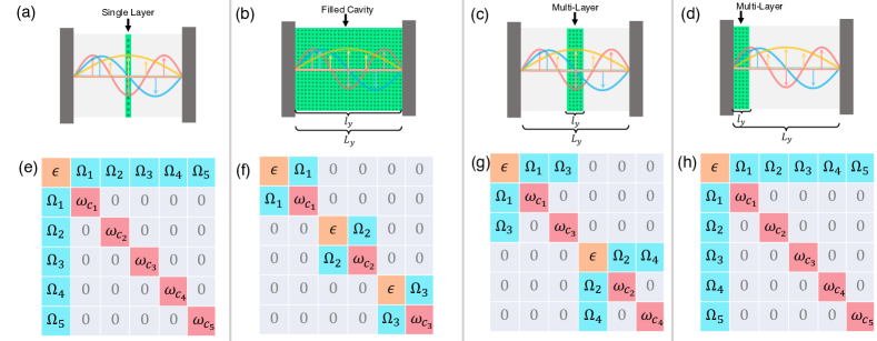
Figure 1: Schematic illustration of various cavity setups in (a)-(d) and their corresponding light-matter matrix in (e)-(h) that can be diagonalized to obtain multi-mode polariton dispersion. The solid green box represents the material of various thicknesses $l_{y}$ and centered at various locations, (a) a single layer material located near the center, (b) material thickness same as the length of the cavity, (c) multi-layer material thickness much smaller than energetically relevant cavity mode wavelengths $l_{y}\ll{2\pi}{k_{y}}$ located at the center of the cavity (d) same as c but located beside one of the cavity mirrors.

Next, we perform a $QR$ decomposition of $\Lambda_{\mathrm{NO}}$ to obtain the orthonormal matrix $\Lambda_{\mathrm{O}}$ (corresponding to $Q$). Using $\Lambda_{\mathrm{O}}$, we define a unitary matrix $U_{\mathrm{O}}$ of dimension $N_{y}\times N_{y}$ such that $[U_{\mathrm{O}}]_{m,j}=[\Lambda_{\mathrm{O}}]_{m,j}$ for $j\in\{n_{\mathrm{min}},n_{\mathrm{min}}+1,...,n_{\mathrm{min}}+N_{e}\}$ and the rest of the matrix elements are chosen such that $\sum_{m}[U_{\mathrm{O}}]_{m,j^{\prime}}\cdot[U_{\mathrm{O}}]_{m,j}=\delta_{jj^{\prime}}$. Using the unitary matrix $U_{\mathrm{O}}$, we define new matter excitation operator as,

$$\hat{d}_{k_{x},k_{y}} =\sum_{m}[U_{\mathrm{O}}]_{m,n_{y}}\cdot\hat{d}_{k_{x},m},$$ (3)

where the index $k_{y}=\frac{\pi}{L_{y}}n_{y}$. The consequence of this transformation is that for $N$ energetically relevant cavity modes, there are $N_{e}\leq N$ matter excitation operators $\{\hat{d}_{k_{x},k_{y}}\}$, such that $k_{y}\in\{n_{\mathrm{min}}\frac{\pi}{L_{y}},...,(n_{\mathrm{min}}+N_{e})\frac{\pi}{L_{y}}\}\equiv\mathcal{N}_{c}$, which couples to the photon operators $\{\hat{a}_{k_{x},k_{y}}\}$. The rest of the matter excitation operators $\{\hat{d}_{k_{x},k_{y}}\}$ for which $k_{y}\notin\mathcal{N}_{c}$ are dark and can be dropped from the light-matter Hamiltonian. The Hamiltonian ${\hat{h}}_{\mathrm{GTC}}(k_{x})$ can be written (using Eqn. Microscopic Theory of Multimode Polariton Dispersion in Multilayered Materials)

$${\hat{h}}_{\mathrm{GTC}} (k_{x})=\sum_{{k_{y}\in\mathcal{K}_{c}}}\hat{a}_{{k_{x},k_{y}}}^{\dagger}\hat{a}_{{k_{x},k_{y}}}\omega_{c}({k_{x},k_{y}})+\epsilon(k_{x})\hat{d}^{\dagger}_{k_{x},k_{y}}\hat{d}_{k_{x},k_{y}}$$

$$+ \sum_{k_{y^{\prime}}\in{\mathcal{N}_{c}}}\sum_{k_{y}\in{\mathcal{K}_{c}}}\Omega({k_{y},k_{y^{\prime}}})\big{(}\hat{a}_{k_{x},k_{y}}^{\dagger}\hat{d}_{k_{x},k_{y^{\prime}}}+\hat{a}_{{k_{x},k_{y}}}\hat{d}_{k_{x},k_{y^{\prime}}}^{\dagger}\big{)},$$ (4)

where

$$\Omega({k_{y},k_{y^{\prime}}})={g_{k_{x},k_{y}}}\sum_{m}\sin(k_{y}Y_{m})\cdot[U_{\mathrm{O}}]_{m,n_{y^{\prime}}}.$$ (5)

Here, $\mathcal{K}_{c}\equiv\{n_{\mathrm{min}}\frac{\pi}{L_{y}},(n_{\mathrm{min}}+1)\frac{\pi}{L_{y}},...,n_{\mathrm{max}}\frac{\pi}{L_{y}}\}$ defines the subspace of energetically relevant cavity operators. Note the relation $\mathcal{N}_{c}\subset\mathcal{K}_{c}$, where $\mathcal{N}_{c}$ is constructed such that columns of $\Lambda_{\mathrm{NO}}$ are linearly independent (in most cases $\mathcal{N}_{c}\equiv\mathcal{K}_{c}$ and $N=N_{e}$).

A general $(N+N_{e})\times(N+N_{e})$ matrix model when using the single excited subspace spanning $\{\hat{a}_{{k_{x},k_{y}}}^{\dagger}|G,0\rangle,\hat{d}_{{k_{x},k_{y}}}^{{}^{\dagger}}|G,0\rangle\}$ (where $|G,0\rangle$ denote the ground state of matter with 0 cavity photons) is obtained as

$${\hat{h}}_{\mathrm{N+N_{e}}}({k_{x}})=$$ (6)

$$\left[\!\begin{array}[]{*{24}{c@{\hspace{2.4pt}}}}\!\epsilon(k_{x})\hfil\hskip&{\Omega}({\frac{\pi n_{1}}{L_{y}},\frac{\pi n_{1}}{L_{y}}})\hfil\hskip&0\hfil\hskip&{\Omega}({\frac{\pi n_{1}}{L_{y}},\frac{\pi n_{2}}{L_{y}}})\hfil\hskip&\ldots\hfil\hskip\\ \!{\Omega}({\frac{\pi n_{1}}{L_{y}},\frac{\pi n_{1}}{L_{y}}})\hfil\hskip&\omega_{c}({k_{x},\frac{\pi n_{1}}{L_{y}}})\hfil\hskip&{\Omega}({\frac{\pi n_{2}}{L_{y}},\frac{\pi n_{1}}{L_{y}}})\hfil\hskip&0\hfil\hskip&\ldots\hfil\hskip\\ \!0\hfil\hskip&{\Omega}({\frac{\pi n_{2}}{L_{y}},\frac{\pi n_{1}}{L_{y}}})\hfil\hskip&\epsilon(k_{x})\hfil\hskip&{\Omega}({\frac{\pi n_{1}}{L_{y}},\frac{\pi n_{2}}{L_{y}}})\hfil\hskip&\ldots\hfil\hskip\\ \!{\Omega}({\frac{\pi n_{1}}{L_{y}},\frac{\pi n_{2}}{L_{y}}})\hfil\hskip&0\hfil\hskip&{\Omega}({\frac{\pi n_{1}}{L_{y}},\frac{\pi n_{2}}{L_{y}}})\hfil\hskip&\omega_{c}({k_{x},\frac{\pi n_{2}}{L_{y}}})\hfil\hskip&\ldots\hfil\hskip\\ \!\vdots\hfil\hskip&\vdots\hfil\hskip&\vdots\hfil\hskip&\vdots\hfil\hskip&\ddots\hfil\hskip\end{array}\!\right].$$ (12)

Note that when $N_{e}=1$, the above matrix reduces to the $(N+1)\times(N+1)$ form ^{35, 31} (such as for a single-layer material). Meanwhile, when $N_{e}=N$ and for ${\Omega}({\frac{\pi m}{L_{y}},\frac{\pi n}{L_{y}}})=\delta_{m,n}{\Omega}({\frac{\pi n}{L_{y}},\frac{\pi n}{L_{y}}})$, the above matrix reduces to the $2N\times 2N$ (such as for a filled cavity) form ^{27, 26, 31}.

In Fig.1 we briefly summarize the schematic forms of the Hamiltonian for various cavity setups that can be diagonalized to obtain the polariton dispersion. Using the general strategy outlined above, for a single layer material shown in Fig. 1e, we find the widely used $(N+1)\times(N+1)$ matrix ^{36, 37, 28, 27, 26, 31, 38, 39}. In this model, within each $k_{x}$ block, one exciton state, corresponding to $\hat{d}_{k_{x},m=0}^{\dagger}|G,0\rangle$, is coupled to $N$ cavity excitations $\hat{a}_{k_{x},k_{y}}^{\dagger}|G,0\rangle$ via the coupling ${\Omega}_{n_{y}}=g_{\boldsymbol{k}}\sin(\frac{\pi n_{y}}{L_{z}}\cdot Y_{0})$ where $Y_{0}$ is the position of the single layer inside cavity.

For a filled cavity, we obtain an $2N\times 2N$ matrix that include $N$ exciton states $\hat{d}_{k_{x},k_{y}}^{\dagger}|G,0\rangle$ where $\hat{d}_{k_{x},k_{y}}^{\dagger}=\frac{1}{\sqrt{\mathcal{N}_{y}}}\sin(k_{y}\cdot(m-\frac{1}{2}))\hat{d}_{k_{x},m}^{\dagger}$ with $\mathcal{N}_{y}$ as a normalization constant, that are coupled to $N$ cavity excitations $\hat{a}_{k_{x},k_{y}}^{\dagger}|G,0\rangle$. This $2N\times 2N$ matrix model contains $N$ non-interacting $2\times 2$ blocks as shown in Fig. 1f. Therefore, in a filled cavity there exists $N$ exciton that couple to $N$ cavity modes of matching $k_{y}$. We also obtain the same $2N\times 2N$ model when considering interacting layers $\tau_{y}\neq 0$ (see detailed analytical expressions in the SI).

For partially filled cavities we find two interesting matrix models depending on the position of the material inside a cavity. For a thin material placed at the middle of the cavity we find a $(N+2)\times(N+2)$ matrix (Fig. 1g) model which is composed of two isolated $(\frac{N}{2}+1)\times(\frac{N}{2}+1)$ blocks. One block contains one ‘symmetric’ exciton state $\hat{d}_{k_{x},\mathrm{S}}^{\dagger}|G,0\rangle$ where $\hat{d}_{k_{x},\mathrm{S}}^{\dagger}=\frac{1}{\sqrt{N_{y}}}\sum_{m}\hat{d}^{\dagger}_{k_{x},m}$ is coupled to odd cavity modes ($k_{y}=\frac{n_{y}\pi}{L_{z}}$ with $n_{y}=2,4,6...$). The other block contain one ‘asymmetric’ exciton state $\hat{d}_{k_{x},\mathrm{A}}^{\dagger}|G,0\rangle$ where $\hat{d}_{k_{x},\mathrm{A}}^{\dagger}=\frac{1}{\sqrt{\mathcal{N}}}\sum_{m}\big{(}Y_{m}-\frac{L_{y}}{2}\big{)}\hat{d}^{\dagger}_{k_{x},m}$ that is coupled to even cavity modes. For a thin material placed next to a mirror, we obtain the $(N+1)\times(N+1)$ model which is shown in Fig. 1h. In this model one exciton state $\hat{d}_{k_{x},B}^{\dagger}|G,0\rangle$ where $\hat{d}_{k_{x},B}={\frac{1}{\sqrt{\mathcal{N}_{B}}}}\sum_{m}Y_{m}\hat{d}_{k_{x},m}$ ($\mathcal{N}_{B}$ is a normalization constant) is coupled to $N$ cavity modes. Note that despite this matrix model being structurally similar to the case of a single layer, the analytical forms of the couplings are quite different and are provided in the SI.

Figure 2: Polariton dispersion for thin material placed (a)-(b) near a cavity mirror, (c)-(d) placed in the middle and a (e)-(f) filled cavity. (a), (c) and (e) Polariton dispersion computed from the generalized Tavis-Cummings Hamiltonian compared to the $(N+1)\times(N+1)$ model in (a), $(N+2)\times(N+2)$ model in (c) and $2N\times 2N$ model in (e). Corresponding absorption spectra for the coupled molecule-cavity hybrid system in (b), (d) and (f).

Numerical Results. Fig. 2 presents numerical results for various multi-layered materials. In Fig. 2a-d we consider a thin material which is either placed next to a mirror (Fig. 2a-b) or in the middle of the cavity (Fig. 2c-d). We choose $L_{y}=20000$ a.u. and a thickness $l_{y}=\delta l_{y}\cdot N_{y}=2000\ll L_{y}$ with $\delta l_{y}=20$ a.u. and $N_{y}=100$. The light-matter coupling used in Fig. 2a-d is $g_{c}=5$ meV, where $g_{\mathrm{k}}=\sqrt{\frac{\omega_{c}({k_{x},k_{y}})}{\omega_{c}(0,\pi/L_{y})}}g_{c}$, and for the matter parameters we choose $\omega_{0}=2.2$ eV with $\tau_{x}=150$ cm^-1. The position of each layer of matter is given by $Y_{m}=(m+\frac{1}{2}){\delta l_{y}}$. Here, we include five energetically relevant cavity modes with $k_{y}\leq 5\frac{\pi}{L_{y}}$.

Fig. 2a shows that the $(N+1)\times(N+1)$ model shown in Fig. 1g (see details in Eqn. S24 in the SI) provides visually identical results compared to direct diagonalization of $\mathcal{H}_{\mathrm{GTC}}(k_{z}=0)$ given in Eqn. Microscopic Theory of Multimode Polariton Dispersion in Multilayered Materials. Note that direct diagonalization also shows the dark matter states which we ignore while constructing $(N+1)\times(N+1)$ model. These dark states do not show up in the absorption (visibility) spectrum as they do not have any photonic contributions. This can be observed in Fig. 2b, which presents the absorption spectrum ^{40, 29} of the coupled cavity-matter system given by

$$I_{\mathrm{A}}(\omega,k_{x})=\sum_{i}|\langle P_{i,k_{x}}|\sum_{k_{y}}\hat{a}^{\dagger}_{k_{x},k_{y}}|G,0\rangle|^{2}e^{-\frac{(\mathcal{E}_{i,k_{x}}-E_{G}-\omega)^{2}}{2\Gamma_{c}^{2}}},$$ (13)

where $|P_{i,k_{x}}\rangle$ is the ith polaritonic state that is an eigenstate of $\hat{h}_{\mathrm{GTC}}(k_{x})$ with energy $\mathcal{E}_{i,k_{x}}$, and $E_{G}$ is the energy of $|G,0\rangle$. Here $\Gamma_{c}=15$ meV is a broadening parameter that is chosen to account for various sources of dissipation phenomenologically, such as cavity loss.

In Fig. 2c-d we consider a material placed in the middle of the cavity such that $Y_{m}=\frac{L_{y}}{2}-\frac{l_{y}}{2}+m\cdot\delta l_{y}$. Fig. 2c show that the $({N}+2)\times({N}+2)$ model shown in Fig. 1f (with details provided in Eqns. S30-S31) correctly predicts the polariton bands in comparison to the numerical results obtained by directly diagonalizing $\hat{h}_{\mathrm{GTC}}({k_{x}})$. Note that in Fig. 2a-b the anti-crossings grow gradually larger with respect to the $k_{y}$ of the cavity mode (which scales as $k_{y}^{3/2}$ as shown in the SI). By contrast, Fig. 2c-d shows that the anti-crossings are large for odd $k_{y}$ while they are negligible for even $k_{y}$, as the spatial dependence for even cavity modes becomes zero at the center of the cavity. Thus, the location of the material inside the cavity plays a crucial role in setting the polariton dispersion.

Fig. 2e-f presents the dispersion and absorption spectra for a filled cavity. Here, we use $g_{c}=2$ meV and use $N_{y}=999$ with $Y_{0}=\frac{\delta l_{y}}{2}=10$ and the rest of the parameters are maintained as in Fig. 2a-d. Fig. 2e presents the corresponding multimode polariton dispersion computed numerically by diagonalizing Eq. Microscopic Theory of Multimode Polariton Dispersion in Multilayered Materials compared with the $2N\times 2N$ model in Eqn. S19. The $2N\times 2N$ model reproduces the band dispersion, as expected. Overall, the results in Fig. 2 demonstrates the validity of the approximate semi-analytical models which are suitable for specific position and properties of the multi-layered material inside the cavity.

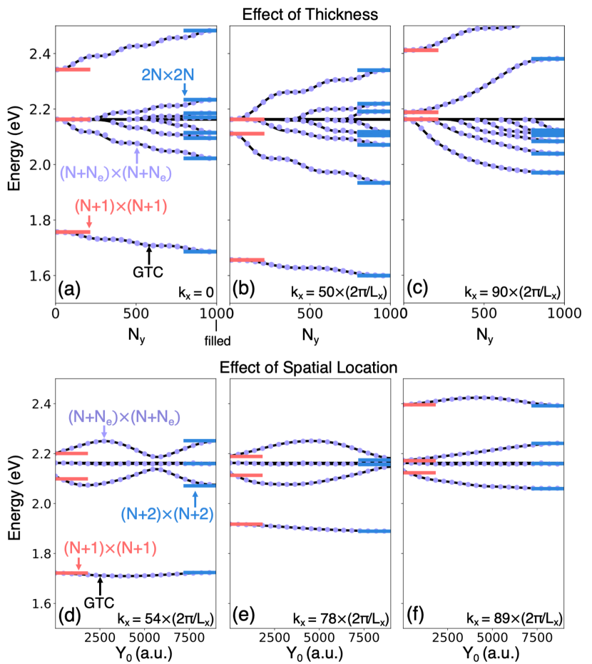
Figure 3: (a)-(c) Polariton dispersion as a function of the number of layers $N_{y}$ at various $k_{x}$ computed from generalized Tavis-Cummings (GTC) Hamiltonian compared to the predictions of the generalized $2N\times 2N$ (at $N_{y}=999$) model and the $(N+1)\times(N+1)$ (at $N_{y}=1$). (d)-(f) Polariton dispersion as a function of the position of the material inside cavity ($Y_{0}$ is the position of the first layer of the material) at various $k_{x}$ computed from generalized Tavis-Cummings (GTC) Hamiltonian compared to the predictions of $(N+1)\times(N+1)$ and $(N+2)\times(N+2)$ model.

In Fig. 3 we explore how the spatial location and the thickness of the material modifies the polariton dispersion. In Fig. 3a-c we explore the dependence of the polariton dispersion on material thickness by plotting polariton bands as a function of $N_{y}$ (number of layers) at various $k_{x}$ values while keeping $g_{c}=4.743$ meV a constant. Our numerical results show that the polariton dispersion at the two limiting extremes, $N_{y}=1$ (single layer) and $N_{y}=999$ (filled), can be obtained using the $(N+1)\times(N+1)$ and the $2N\times 2N$ models, respectively. For any intermediate values of $N_{y}$, i.e. partially filled cavities, accurate polariton dispersion can be obtained using the general $(N+N_{e})\times(N+N_{e})$ model (compare the violet dots with the black solid lines) given in Eqn. 6.

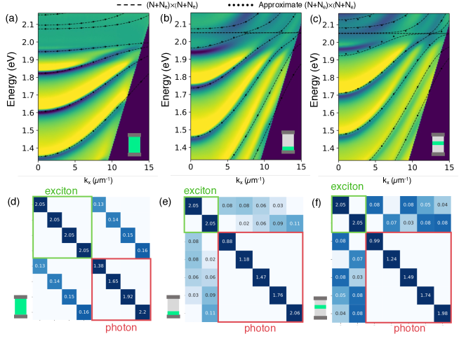
Figure 4: (a)-(c) Comparing experimental dispersion for three different structure (a) filled cavity, (b) material placed at the beside a mirror and (c) material placed near the middle of the cavity. The experimental results are compared to theoretical predictions with dashed line represents the predictions using the general $(N+N_{e})\times(N+N_{e})$ model and the dotted lines represents the predictions using the approximate $(N+N_{e})\times(N+N_{e})$ model. (d)-(e) The matrix structure of the approximate $(N+N_{e})\times(N+N_{e})$ model corresponding to (a)-(c) with values in eV.

Similarly, Fig. 3d-f presents the polariton bands at three specific value of $k_{x}$ and as a function of the material location $Y_{0}$. Here we use $g_{c}=4.743$ meV while the rest of parameters are the same as in Fig. 2a. The numerical results show that the in the limiting scenarios, at $Y_{0}=\frac{\delta l_{y}}{2}=10$ a.u. and $Y_{0}=\frac{L_{y}-l_{y}}{2}=9000$ a.u., the polariton dispersion can be obtained by the $(N+2)\times(N+2)$ and by $({N}+1)\times({N}+1)$ models, respectively.

Overall, we numerically demonstrate that the general $(N+N_{e})\times(N+N_{e})$ model can be used to compute the multimode polariton dispersion for arbitrary geometries of multi-layered materials. We demonstrated that in specific scenarios, simplified models such as $2N\times 2N$, $(N+1)\times(N+1)$ and $(N+2)\times(N+2)$ model can be used to compute the polariton dispersion. Our work sheds light on the recently discussed ambiguity ^{26, 31, 27, 41, 42, 43} of using $(N+1)\times(N+1)$ and $2N\times 2N$ models for fitting experimental dispersion. While for single-layer thin materials the $(N+1)\times(N+1)$ model is appropriate, the $2N\times 2N$ model is appropriate for obtaining polariton dispersions in filled cavities. However, our result suggest that the general $(N+N_{e})\times(N+N_{e})$ model should be used in all circumstances for extracting parameters related to light-matter coupling.

Comparison with Experiment. Here we implement the general $(N+N_{e})\times(N+N_{e})$ model to compute the multimode polariton dispersion for a multi-layered perovskite material and compare to the experimentally obtained reflectance spectrum. We prepare a multi-layered 2D perovskite material BA₂(MA)₂Pb₃I₁₀, where BA = CH₃(CH₂)₃NH₃ and MA = CH₃NH₃ that is sandwiched between an Ag and Au layer that act as mirrors. We also use a Poly(methyl methacrylate) (PMMA) layer as a spacer to extend the quantization length of the cavity when making partially filled cavities. Experimental details can be found in the SI. Note that the layers of the perovskite material can be considered non-interacting, thus allowing us to directly implement the general $(N+N_{e})\times(N+N_{e})$ model to obtain the multimode polariton dispersion.

Fig. 4 presents the multimode polariton dispersion obtained experimentally via the reflectance spectra. Fig. 4a shows the reflectance spectra obtained for filled cavity. To obtain the theoretical multimode polariton dispersion we model the matter as a dispersionless material with a matter excitation energy of $\omega_{0}=2.05$ eV (such that $\epsilon(k_{x})=\omega_{0}$) and a refractive index of $\eta_{\mathrm{PX}}=2.2$. ⁴⁴ We directly use this refractive index to obtain the uncoupled photon band dispersion $\omega_{\mathrm{c}}({\boldsymbol{k}})=\frac{c}{\eta}|\boldsymbol{k}|$ for the filled cavity presented in Fig. 4a. We use an individual layer thickness of $\delta l_{y}=50$ a.u. ⁴⁵ Note that for $\delta l_{y}\ll l_{y}$ (that is for large $N_{y}$), the explicit value of the $\delta l_{y}$ does not matter. We find $g_{c}\approx 4.2$ meV (such that $g_{\mathrm{k}}=\sqrt{\frac{\omega_{c}({k_{x},k_{y}})}{\omega_{c}(0,\pi/L_{y})}}g_{c}$) and $L_{y}\approx 19358$ a.u. through fitting and consider the 4th to 7th cavity mode branch along $y$, that is $k_{y}\in\{\frac{4\pi}{L_{y}},\frac{5\pi}{L_{y}},\frac{6\pi}{L_{y}},\frac{7\pi}{L_{y}}\}$, for constructing the general $(N+N_{e})\times(N+N_{e})$ matrix. In addition to this we can also construct approximate $(N+N_{e})\times(N+N_{e})$ models by ignoring weakly coupled excitonic branches. A numerical way to perform this approximation is by using a tolerance factor $\epsilon_{\mathrm{tol}}$ (set to 0.1 here) below which the singular values are considered to be 0 when checking for linear independence via the use of Eqn. 2 for constructing $\Lambda_{\mathrm{NO}}$. The dispersion obtained with the general $(N+N_{e})\times(N+N_{e})$ model (dashed lines) and the approximate $(N+N_{e})\times(N+N_{e})$ model (black circles) is overlayed on the experimentally obtained reflectance in Fig. 4a-c. These results show that our theoretical model is able to fit the experimental dispersion very well. Note that the upper polariton branches are not visible in the experimental dispersion for this structure because the thick semiconductor absorbs too much above-gap light ^{46, 47}.

In Fig. 4a only two parameters $g_{c}$ and $L_{y}$ are used for fitting the experimental dispersion. As can be seen, these parameters provide accurate band dispersion compared to the experimental results. The numerically computed approximate $(N+N_{e})\times(N+N_{e})$ matrix model at $k_{x}=0$ is shown in Fig, 4d, which exactly takes the form of the widely used $2N\times 2N$ model^{28, 27, 26, 31}.

Next in Fig. 4b we manufacture a partially filled cavity by using PMMA as a spacer. The refractive index of the PMMA is $\eta_{\mathrm{PMMA}}$ = 1.5. For a cavity filled with materials of different refractive index, we obtain an effective refractive index through fitting such that $1.5<\eta<2.2$. Here we obtain, the length of the perovskite material $l_{y}=5550$ a.u., the length of the cavity $L_{y}\approx 24142$ a.u., $g_{c}\approx 5.39$ meV and the effective refractive index $\eta$ = 1.65 by fitting the dispersion curves visually. Here we have considered five energetically relevant cavity mode branches (the 3rd to 7th cavity mode branch along $y$) with $k_{y}\in\{\frac{3\pi}{L_{y}},\frac{4\pi}{L_{y}},\frac{5\pi}{L_{y}},\frac{6\pi}{L_{y}},\frac{7\pi}{L_{y}}\}$. These parameters fit the dispersion with reasonable accuracy. The numerically computed approximate $(N+N_{e})\times(N+N_{e})$ matrix at $k_{x}=0$ is shown in Fig, 4e for the case shown in Fig, 4b. As can be seen here, the matrix has a $(N+2)\times(N+2)$ structure with a very complex set of couplings between the cavity and exciton branches.

Finally, in Fig. 4c we show results after fabrication of partially filled cavities with the material placed near the center of the cavity. Here, we fit and obtain $L_{y}=$ 28278 a.u., $l_{y}=$ 4500 a.u., $\eta$ = 1.67, $g_{c}\approx 5.146$ meV and additionally find the location of the material $Y_{0}=5.1\times L_{y}$, by visually fitting the dispersion. Here we have considered five energetically relevant cavity mode branches (3rd to 7th cavity mode branch along $y$). The corresponding approximate $(N+N_{e})\times(N+N_{e})$ matrix at $k_{x}=0$ is shown in Fig. 4e for the case shown in Fig. 4f which, similar to the previous case, has a $(N+2)\times(N+2)$ structure with a complex set of couplings. In all cases we capture all of the subtle features of the experimental dispersion with reasonable accuracy.

Conclusions. In this work we have presented a microscopic theory for obtaining multimode polariton dispersion of a material inside a cavity. Starting with the GTC Hamiltonian, we develop a general strategy to obtain the polariton dispersion in multimode cavities, which takes the form of a general $(N+N_{e})\times(N+N_{e})$ model. Unlike the widely used $2N\times 2N$ or $(N+1)\times(N+1)$ models, our approach can be used for a material of arbitrary thickness and position within the cavity to obtain the multimode polariton dispersion. In contrast to previous approaches of directly fitting matrix elements, our method relies on structural parameters like the thickness and location of the material inside the cavity. We show that in certain limiting scenarios, the general $(N+N_{e})\times(N+N_{e})$ model reduces to the widely used $2N\times 2N$ (for a filled cavity) model or the $(N+1)\times(N+1)$ (single or thin layer placed beside a mirror) model, and find other interesting models such as the $(N+2)\times(N+2)$ model that describes a thin material placed in the middle of the cavity.

While in this work we have employed a simple tight-binding model for the matter, our strategy can be generalized to using ab initio electronic structure theory with multiple bands. In future research, we will extend this approach toward ab initio modeling.

1 Acknowledgements

This work was supported by NSF-1954791 (A.M. and D.R.R.) and NSF CHE-2203844 (M.E.D. and D.X.). We acknowledge the services provided by XSEDE (TG-CHE210085) and the OSG Consortium ^{48, 49}, supported by the NSF awards $\#$2030508 and $\#$1836650.

References

- Hutchison et al. 2012 Hutchison, J. A.; Schwartz, T.; Genet, C.; Devaux, E.; Ebbesen, T. W. Modifying Chemical Landscapes by Coupling to Vacuum Fields. Angew. Chem. Int. Ed. 2012, 51, 1592–1596
- Feist et al. 2018 Feist, J.; Galego, J.; Garcia-Vidal, F. J. Polaritonic Chemistry with Organic Molecules. ACS Photonics 2018, 5, 205–216
- Thomas et al. 2019 Thomas, A.; Lethuillier-Karl, L.; Nagarajan, K.; Vergauwe, R. M. A.; George, J.; Chervy, T.; Shalabney, A.; Devaux, E.; Genet, C.; Moran, J. et al. Tilting a ground-state reactivity landscape by vibrational strong coupling. Science 2019, 363, 615–619
- Garcia-Vidal et al. 2021 Garcia-Vidal, F. J.; Ciuti, C.; Ebbesen, T. W. Manipulating matter by strong coupling to vacuum fields. Science 2021, 373
- Nagarajan et al. 2021 Nagarajan, K.; Thomas, A.; Ebbesen, T. W. Chemistry under Vibrational Strong Coupling. J. Am. Chem. Soc. 2021, 143, 16877–16889
- Ribeiro et al. 2018 Ribeiro, R. F.; Martínez-Martínez, L. A.; Du, M.; Gonzalez-Angulo, J. C.; Yuen-Zhou, J. Polariton chemistry: controlling molecular dynamics with optical cavities. Chem. Sci. 2018, 9, 6325–6339
- Mandal et al. 2020 Mandal, A.; Krauss, T. D.; Huo, P. Polariton-Mediated Electron Transfer via Cavity Quantum Electrodynamics. J. Phys. Chem. B 2020, 124, 6321–6340
- Semenov and Nitzan 2019 Semenov, A.; Nitzan, A. Electron transfer in confined electromagnetic fields. J. Chem. Phys. 2019, 150, 174122
- Wu et al. 2022 Wu, W.; Sifain, A. E.; Delpo, C. A.; Scholes, G. D. Polariton enhanced free charge carrier generation in donor–acceptor cavity systems by a second-hybridization mechanism. J. Chem. Phys. 2022, 157, 161102
- Mandal et al. 2022 Mandal, A.; Taylor, M.; Weight, B.; Koessler, E.; Li, X.; Huo, P. Theoretical Advances in Polariton Chemistry and Molecular Cavity Quantum Electrodynamics. ChemRxiv 2022,
- Li et al. 2021 Li, T. E.; Cui, B.; Subotnik, J. E.; Nitzan, A. Molecular Polaritonics: Chemical Dynamics Under Strong Light–Matter Coupling. Annu. Rev. Phys. Chem. 2021, 73
- Berghuis et al. 2022 Berghuis, A. M.; Tichauer, R. H.; de Jong, L. M. A.; Sokolovskii, I.; Bai, P.; Ramezani, M.; Murai, S.; Groenhof, G.; Rivas, J. G. Controlling Exciton Propagation in Organic Crystals through Strong Coupling to Plasmonic Nanoparticle Arrays. ACS Photonics 2022, 9, 2263–2272
- Xu et al. 2022 Xu, D.; Mandal, A.; Baxter, J. M.; Cheng, S.-W.; Lee, I.; Su, H.; Liu, S.; Reichman, D. R.; Delor, M. Ultrafast imaging of coherent polariton propagation and interactions. arXiv 2022,
- Deng et al. 2010 Deng, H.; Haug, H.; Yamamoto, Y. Exciton-polariton Bose-Einstein condensation. Rev. Mod. Phys. 2010, 82, 1489–1537
- Kockum et al. 2019 Kockum, A. F.; Miranowicz, A.; Liberato, S. D.; Savasta, S.; Nori, F. Ultrastrong coupling between light and matter. Nat. Rev. Phys. 2019, 1, 19–40
- Keeling and Kéna-Cohen 2020 Keeling, J.; Kéna-Cohen, S. Bose–Einstein Condensation of Exciton-Polaritons in Organic Microcavities. Ann. Rev. Phys. Chem. 2020, 71, 435–459
- Arnardottir et al. 2020 Arnardottir, K. B.; Moilanen, A. J.; Strashko, A.; Törmä, P.; Keeling, J. Multimode Organic Polariton Lasing. Phys. Rev. Lett. 2020, 125, 233603
- Rozenman et al. 2018 Rozenman, G. G.; Akulov, K.; Golombek, A.; Schwartz, T. Long-Range Transport of Organic Exciton-Polaritons Revealed by Ultrafast Microscopy. ACS Photonics 2018, 5, 105–110
- Perez-Sanchez and Yuen-Zhou 2020 Perez-Sanchez, J. B.; Yuen-Zhou, J. Polariton Assisted Down-Conversion of Photons via Nonadiabatic Molecular Dynamics: A Molecular Dynamical Casimir Effect. J. Phys. Chem. Lett. 2020, 11, 152–159
- Mandal et al. 2020 Mandal, A.; Vega, S. M.; Huo, P. Polarized Fock States and the Dynamical Casimir Effect in Molecular Cavity Quantum Electrodynamics. J. Phys. Chem. Lett. 2020, 11, 9215–9223
- Sanchez-Barquilla et al. 2022 Sanchez-Barquilla, M.; Fernandez-Dominguez, A. I.; Feist, J.; Garcia-Vidal, F. J. A Theoretical Perspective on Molecular Polaritonics. ACS Photonics 2022, 9, 1830–1841
- Reithmaier et al. 2004 Reithmaier, J. P.; Sek, G.; Löffler, A.; Hofmann, C.; Kuhn, S.; Reitzenstein, S.; Keldysh, L.; Kulakovskii, V.; Reinecke, T.; Forchel, A. Strong coupling in a single quantum dot–semiconductor microcavity system. Nature 2004, 432, 197–200
- Müller et al. 2015 Müller, K.; Fischer, K. A.; Rundquist, A.; Dory, C.; Lagoudakis, K. G.; Sarmiento, T.; Kelaita, Y. A.; Borish, V.; Vučković, J. Ultrafast Polariton-Phonon Dynamics of Strongly Coupled Quantum Dot-Nanocavity Systems. Phys. Rev. X 2015, 5, 031006
- Laussy et al. 2012 Laussy, F. P.; del Valle, E.; Schrapp, M.; Laucht, A.; Finley, J. J. Climbing the Jaynes-Cummings ladder by photon counting. J. Nanophotonics 2012, 6, 061803
- Deng et al. 2003 Deng, H.; Weihs, G.; Snoke, D.; Bloch, J.; Yamamoto, Y. Polariton lasing vs. photon lasing in a semiconductor microcavity. Proc. Natl. Acad. Sci. U.S.A. 2003, 100, 15318–15323
- Georgiou et al. 2021 Georgiou, K.; McGhee, K. E.; Jayaprakash, R.; Lidzey, D. G. Observation of photon-mode decoupling in a strongly coupled multimode microcavity. J. Chem. Phys. 2021, 154, 124309
- Richter et al. 2015 Richter, S.; Michalsky, T.; Fricke, L.; Sturm, C.; Franke, H.; Grundmann, M.; Schmidt-Grund, R. Maxwell consideration of polaritonic quasi-particle Hamiltonians in multi-level systems. App. Phys. Lett. 2015, 107, 231104
- Michetti and La Rocca 2005 Michetti, P.; La Rocca, G. Polariton states in disordered organic microcavities. Physical Review B 2005, 71, 115320
- Tichauer et al. 2021 Tichauer, R. H.; Feist, J.; Groenhof, G. Multi-scale dynamics simulations of molecular polaritons: The effect of multiple cavity modes on polariton relaxation. J. Chem. Phys. 2021, 154, 104112
- Gerace and Andreani 2007 Gerace, D.; Andreani, L. C. Quantum theory of exciton-photon coupling in photonic crystal slabs with embedded quantum wells. Physical Review B 2007, 75, 235325
- Balasubrahmaniyam et al. 2021 Balasubrahmaniyam, M.; Genet, C.; Schwartz, T. Coupling and decoupling of polaritonic states in multimode cavities. Physical Review B 2021, 103, L241407
- Keeling 2012 Keeling, J. Light-Matter Interactions and Quantum Optics; University of St. Andrews, 2012
- Li et al. 2020 Li, J.; Golez, D.; Mazza, G.; Millis, A. J.; Georges, A.; Eckstein, M. Electromagnetic coupling in tight-binding models for strongly correlated light and matter. Phys. Rev. B 2020, 101, 205140
- Dmytruk and Schiró 2021 Dmytruk, O.; Schiró, M. Gauge fixing for strongly correlated electrons coupled to quantum light. Phys. Rev. B 2021, 103, 075131
- Graf et al. 2016 Graf, A.; Tropf, L.; Zakharko, Y.; Zaumseil, J.; Gather, M. C. Near-infrared exciton-polaritons in strongly coupled single-walled carbon nanotube microcavities. Nature Communications 2016, 7, 13078
- Dietrich et al. 2016 Dietrich, C. P.; Steude, A.; Tropf, L.; Schubert, M.; Kronenberg, N. M.; Ostermann, K.; Höfling, S.; Gather, M. C. An exciton-polariton laser based on biologically produced fluorescent protein. Science advances 2016, 2, e1600666
- Coles and Lidzey 2014 Coles, D. M.; Lidzey, D. G. A ladder of polariton branches formed by coupling an organic semiconductor exciton to a series of closely spaced cavity-photon modes. Applied Physics Letters 2014, 104, 191108
- Orosz et al. 2011 Orosz, L.; Reveret, F.; Bouchoule, S.; Zúñiga-Pérez, J.; Médard, F.; Leymarie, J.; Disseix, P.; Mihailovic, M.; Frayssinet, E.; Semond, F. et al. Fabrication and optical properties of a fully-hybrid epitaxial ZnO-based microcavity in the strong-coupling regime. Applied physics express 2011, 4, 072001
- Faure et al. 2009 Faure, S.; Brimont, C.; Guillet, T.; Bretagnon, T.; Gil, B.; Médard, F.; Lagarde, D.; Disseix, P.; Leymarie, J.; Zúñiga-Pérez, J. et al. Relaxation and emission of Bragg-mode and cavity-mode polaritons in a ZnO microcavity at room temperature. Applied Physics Letters 2009, 95, 121102
- Lidzey et al. 2000 Lidzey, D. G.; Bradley, D. D. C.; Armitage, A.; Walker, S.; Skolnick, M. S. Photon-Mediated Hybridization of Frenkel Excitons in Organic Semiconductor Microcavities. Science 2000, 288, 1620–1623
- Georgiou et al. 2021 Georgiou, K.; Jayaprakash, R.; Othonos, A.; Lidzey, D. G. Ultralong-Range Polariton-Assisted Energy Transfer in Organic Microcavities. Angewandte Chemie 2021, 133, 16797–16803
- Menghrajani and Barnes 2020 Menghrajani, K. S.; Barnes, W. L. Strong Coupling beyond the Light-Line. ACS Photonics 2020, 7, 2448–2459, PMID: 33163580
- Tagami et al. 2021 Tagami, T.; Ueda, Y.; Imai, K.; Takahashi, S.; Mizuno, H.; Yanagi, H.; Obuchi, T.; Nakayama, M.; Yamashita, K. Anisotropic light-matter coupling and below-threshold excitation dynamics in an organic crystal microcavity. Optics Express 2021, 29, 26433–26443
- Song et al. 2021 Song, B.; Hou, J.; Wang, H.; Sidhik, S.; Miao, J.; Gu, H.; Zhang, H.; Liu, S.; Fakhraai, Z.; Even, J. et al. Determination of Dielectric Functions and Exciton Oscillator Strength of Two-Dimensional Hybrid Perovskites. ACS Materials Letters 2021, 3, 148–159
- Mao et al. 2018 Mao, L.; Stoumpos, C. C.; Kanatzidis, M. G. Two-dimensional hybrid halide perovskites: principles and promises. J. Am. Chem. Soc. 2018, 141, 1171–1190
- Fieramosca et al. 2019 Fieramosca, A.; Polimeno, L.; Ardizzone, V.; Marco, L. D.; Pugliese, M.; Maiorano, V.; Giorgi, M. D.; Dominici, L.; Gigli, G.; Gerace, D. et al. Two-dimensional hybrid perovskites sustaining strong polariton interactions at room temperature. Science Advances 2019, 5, eaav9967
- Wang et al. 2018 Wang, J.; Su, R.; Xing, J.; Bao, D.; Diederichs, C.; Liu, S.; Liew, T. C.; Chen, Z.; Xiong, Q. Room Temperature Coherently Coupled Exciton–Polaritons in Two-Dimensional Organic–Inorganic Perovskite. ACS Nano 2018, 12, 8382–8389
- Sfiligoi et al. 2009 Sfiligoi, I.; Bradley, D. C.; Holzman, B.; Mhashilkar, P.; Padhi, S.; Wurthwein, F. The pilot way to grid resources using glideinWMS. 2009 WRI World Congress on Computer Science and Information Engineering. 2009; pp 428–432
- Pordes et al. 2007 Pordes, R.; Petravick, D.; Kramer, B.; Olson, D.; Livny, M.; Roy, A.; Avery, P.; Blackburn, K.; Wenaus, T.; Würthwein, F. et al. The open science grid. J. Phys. Conf. Ser. 2007; p 012057