Isoparametric Tangled Finite Element Method for Nonlinear Elasticity

Abstract

An important requirement in the standard finite element method (FEM) is that all elements in the underlying mesh must be tangle-free i.e., the Jacobian must be positive throughout each element. To relax this requirement, an isoparametric tangled finite element method (i-TFEM) was recently proposed for linear elasticity problems. It was demonstrated that i-TFEM leads to optimal convergence even for severely tangled meshes.

In this paper, i-TFEM is generalized to nonlinear elasticity. Specifically, a variational formulation is proposed that leads to local modification in the tangent stiffness matrix associated with tangled elements, and an additional piece-wise compatibility constraint. i-TFEM reduces to standard FEM for tangle-free meshes. The effectiveness and convergence characteristics of i-TFEM are demonstrated through a series of numerical experiments, involving both compressible and in-compressible problems.

myequation

1 Introduction

The finite element method (FEM) is extensively used for solving a wide variety of problems in nonlinear solid mechanics. A crucial step in FEM is meshing, where a finite element mesh is generated to represent the physical domain. An important requirement of a valid FEM mesh is that it should not contain tangled elements [1, 2, 3, 4]. In other words, every element must be fully invertible. However, generating high-quality, tangle-free meshes remains a challenge, despite advances in mesh generation methods [5, 6]. State-of-the-art mesh generation methods [7, 8, 9, 10, 11, 12, 13, 14] can still lead to a tangled mesh. As a result, many untangling techniques have been developed [15, 16, 17, 18, 19], but they are not always reliable. Several instances have been reported where no tangle-free solution could be found without altering the boundary [15, 20, 16].

This paper is focused on handling inverted (i.e., concave) bilinear quadrilateral (Q4) elements, a widely used element in FEM, within the context of nonlinear solid mechanics. Various non-traditional finite element formulations have been proposed to handle concave element shapes; for instance, smoothed finite element [21], polygonal finite elements [22], virtual elements [23], unsymmetrical FEM [24]. These have been applied to solve problems with finite deformations, for instance, PolyFEM [25, 26], VEM [27, 28, 29], unsymmetrical FEM [30]. However, these methods often require significant modifications to FEM (for example, the use of non-standard shape functions) and/or do not reduce to standard FEM for non-tangled (regular) meshes.

Recently, an isoparametric tangled finite element method (i-TFEM) was proposed as an extension to the standard FEM [31] to handle tangled elements for linear problems. The proposed method uses the same shape functions as FEM, reduces to the standard FEM for non-tangled meshes, and maintains the symmetry of the stiffness matrix. In i-TFEM, tangled elements are handled by: (1) locally modifying the elemental stiffness matrices associated with the tangled elements, and (b) enforcing piecewise compatibility constraints at re-entrant nodes. It was demonstrated in the context of tangled quadrilateral (Q4) and 8-node (H-8) hexahedral meshes for linear elasticity and Poisson problems [31, 32, 33].

In this paper, i-TFEM is extended to handle finite deformation problems, with hyperelasticity, over tangled 4-node quadrilateral (Q4) meshes. Towards this end, a mixed formulation for i-TFEM is introduced, and the required modifications to the tangent matrices over the concave elements are formally derived. It is demonstrated that the results obtained over tangled meshes using i-TFEM have the convergence rate comparable to that of the standard FEM with regular meshes. Several examples with compressibility and near-incompressibility are presented to demonstrate the robustness of i-TFEM.

The remainder of this paper is organized as follows. The standard finite element formulation for nonlinear elasticity is reviewed in Section 2; the challenges associated with tangled meshes are highlighted. Section 3 describes the proposed i-TFEM method using total Lagrangian formulation. This is followed by numerical experiments in Section 4, and conclusions in Section 5.

2 Nonlinear elasticity

Consider a body occupying a domain $\Omega\in\mathbb{R}^{2}$ subject to a body force $\boldsymbol{b}$, traction $\boldsymbol{T}$ over the boundary $\partial\Omega^{T}$, and Dirichlet boundary conditions $\boldsymbol{u}=\boldsymbol{u_{d}}$ over the boundary $\partial\Omega^{d}$; the material is assumed to be hyper-elastic undergoing a finite deformation $\boldsymbol{u}$. The domain is divided into $M$ elements $E_{j}$, identified by the set $I=\left\{1,\dots M\right\}$. We employ the total Lagrangian formulation [34] in this paper, where the potential energy can be written as:

$$\Pi(\boldsymbol{u})=\sum_{j\in I}\int\limits_{E_{j}}{\Psi\left(\boldsymbol{F}\left(\boldsymbol{u}_{j}\right)\right)dV}-\sum_{j\in I}\int\limits_{E_{j}}{\boldsymbol{u}_{j}\cdot\boldsymbol{b}dV}-\sum_{j\in I}\int\limits_{\partial E_{j}^{T}}{\boldsymbol{u}_{j}\cdot\boldsymbol{T}dS}$$ (2)

where $\boldsymbol{F}$ is the deformation gradient, $\Psi$ is the strain energy density. Further, using the standard (Bubnov-) Galerkin variational formulation, one arrives at the residual equation [34]:

$$\boldsymbol{R}(\boldsymbol{\hat{u}})=0$$ (3)

This is typically solved iteratively via the Newton-Raphson algorithm [34]:

$$\boldsymbol{K}(\boldsymbol{\hat{u}}^{n})\Delta\boldsymbol{\hat{u}}^{n+1}=-\boldsymbol{R}(\boldsymbol{\hat{u}}^{n}).$$ (4)

where $\boldsymbol{K}$ is the tangent matrix and $\Delta\boldsymbol{\hat{u}}^{n}$ is the incremental displacement vector at $n^{th}$ Newton iteration. When the mesh is of high-quality and not tangled, one obtains accurate solutions to such problems.

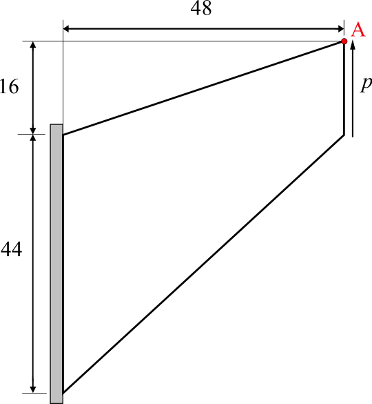
However, as is well known, when the mesh is tangled, i.e., if the mesh contains inverted elements, the solution becomes erroneous. To illustrate, consider Cook’s membrane problem [35] illustrated in Fig. 1(a). The left edge of the tapered cantilever is fixed while a uniformly distributed load $p=5$ is applied on the right edge. We pose a geometrically nonlinear plane-strain problem with Lamé parameters $\mu=50$ and $\lambda=100$. Fig. 1(b) illustrates a quadrilateral mesh with one concave element that we use for this experiment.

(a)

(b)

Figure 1: (a) Cook’s membrane problem. (b) Tangled mesh with one concave element.

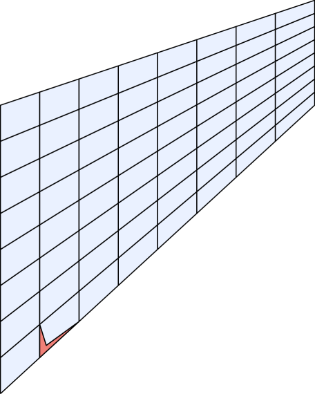
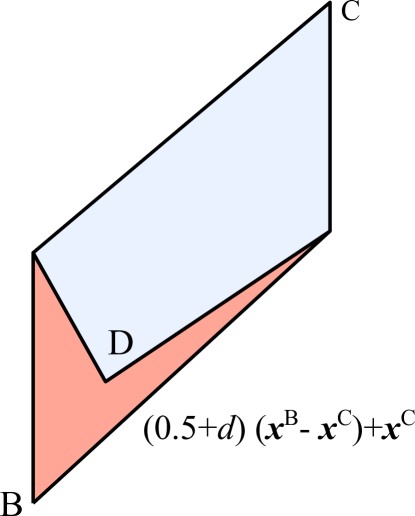
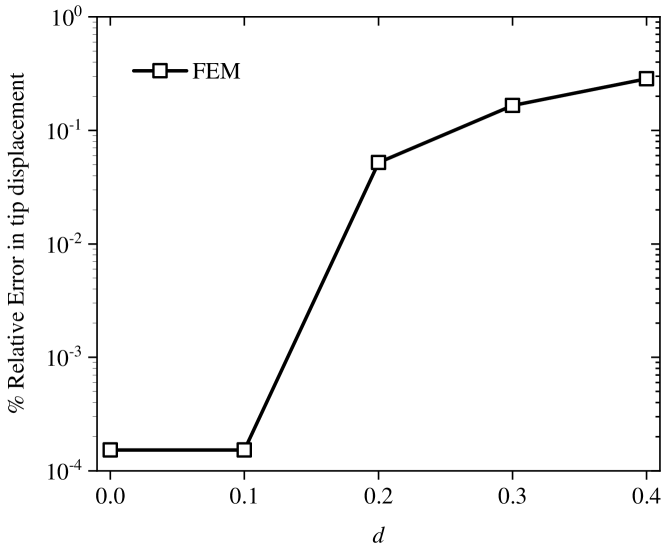
We vary the extent of tangling by moving the re-entrant vertex D along the diagonal BC as shown in Fig. 2(a). When the parameter $d=0$, the point D lies half-way between B and C, and when $0<d<0.5$, the point D moves towards B, i.e., the element gets tangled. The large-deformation problem is solved using the normal procedure as described above, with 10 load steps. The tip displacement is compared against the expected value (using a high quality non-tangled mesh). When $d>0.1$, a negative $|\boldsymbol{J}|$ value is encountered at one or more Gauss points, and Fig. 2(b) illustrates the resulting erroneous solution.

(a)

(b)

Figure 2: (a) Zoomed-in view of the tangled element. (b) Relative error in tip displacement versus $d$ for FEM.

3 Isoparametric TFEM for nonlinear elasticity

The objective of this paper is to propose an iso-parametric tangled finite element method (i-TFEM), as a simple extension to classic FEM, for solving large deformation problems over tangled meshes. As a background, we briefly review the critical i-TFEM concepts proposed in [33] for linear problems.

3.1 Isoparametric TFEM

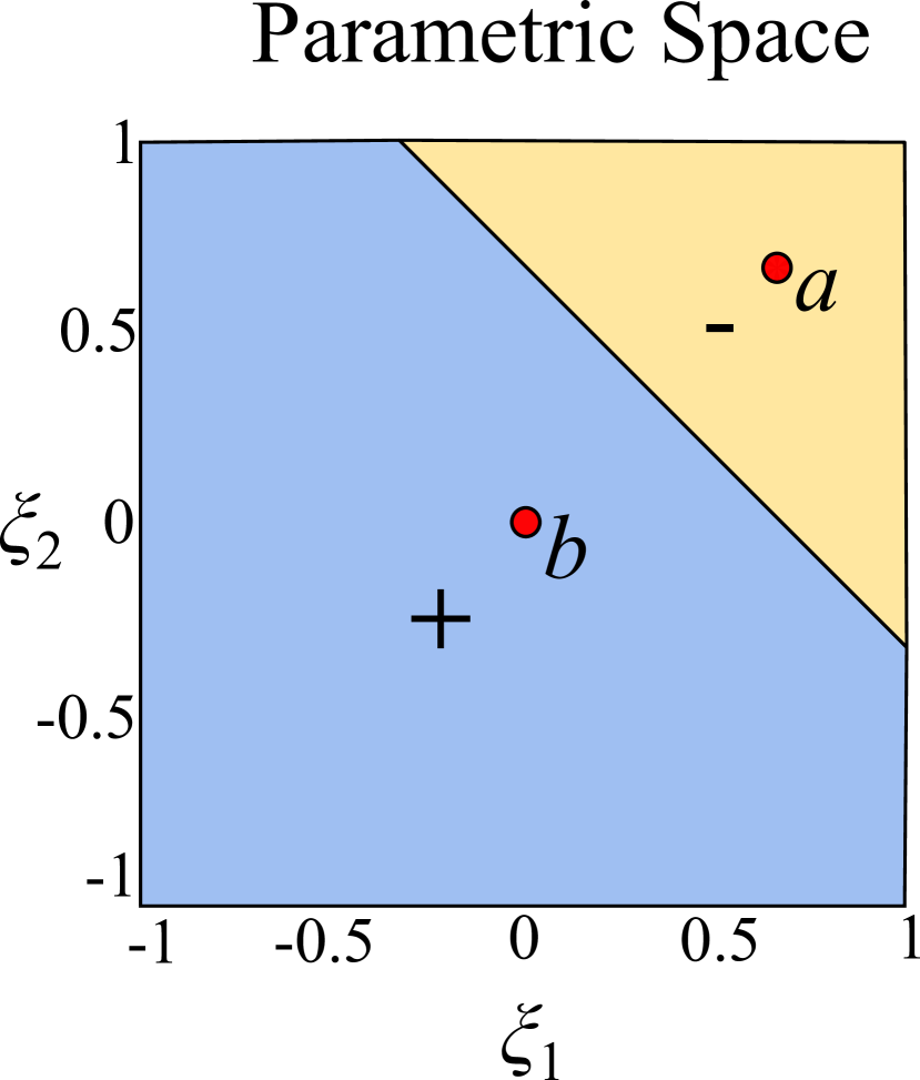
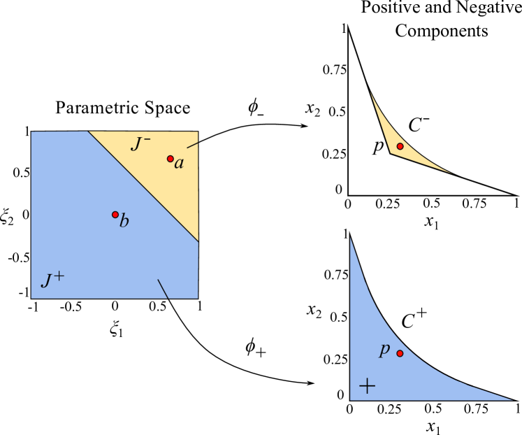
Consider the standard isoparametric mapping from $(\xi_{1},\xi_{2})$ space in Fig. 3(a) to a concave element in the physical space $(x_{1},x_{2})$ in Fig. 3(b). Observe that the element folds onto itself. Further, the parametric space can be divided into positive ($J^{+}$) and negative ($J^{-}$) Jacobian regions and the parametric mapping $\phi$ is not fully invertible.

The main idea in i-TFEM is that the positive and negative parametric regions are treated separately, thus relaxing the constraint of full invertibility to piecewise invertibility. In particular, the physical space corresponding to the positive (negative) parametric region $J^{+}$ ($J^{-}$) is termed as positive (negative) component and is denoted by $C^{+}$ ($C^{-}$). Observe the piecewise mapping

$$\phi_{\pm}\colon J^{\pm}\rightarrow C^{\pm}$$

is invertible i.e. bijective (see Fig. 3(c)).

(a)

(b)

(c)

Figure 3: (a) Parametric space of the concave element. Parametric space can be divided into positive and negative Jacobian regions. (b) Physical space of the concave Q9 element. (c) Positive and negative components

Let $\boldsymbol{N}_{j}(\boldsymbol{\xi})$ be the standard bilinear Lagrange shape functions defined over the parametric space of element $E_{j}$. Let $\boldsymbol{N}_{j}^{\pm}$ be the restriction of $\boldsymbol{N}_{j}$ to $J^{\pm}$, i.e.,

$$\boldsymbol{N}_{j}^{\pm}(\boldsymbol{x})\coloneqq\boldsymbol{N}_{j}(\phi^{-1}_{\pm}(\boldsymbol{x}))$$ (5)

The corresponding field is then given by

$$\boldsymbol{u}_{j}^{\pm}(\boldsymbol{x})=\boldsymbol{N}_{j}^{\pm}(\boldsymbol{x})\boldsymbol{{\hat{u}}}_{j}$$ (6)

Now consider the two-element tangled patch in Fig. 4a. The positive and negative components ($C_{1}^{+}$ and $C_{1}^{-}$) of the concave element $E_{1}$ are shown in Fig. 4b. On the other hand, the convex element $E_{2}$ has only one positive component (see Fig. 4c): $E_{2}=C_{2}^{+}$ while $C_{2}^{-}=\emptyset$. Further, the fold $F_{1}$ illustrated in Fig. 4d overlaps with $E_{2}$ as well.

Figure 4: (a) 2-D domain discretized into two bilinear quads. (b) Positive and negative $|\boldsymbol{J}|$ regions of the concave element. (c) Convex element of the mesh. (d) Final physical space is self-overlapping.

Thus, for any point $\boldsymbol{x}\in F_{1}$, all the three components overlap, and three fields $\boldsymbol{u}^{+}_{1}\left(\boldsymbol{x}\right)$, $\boldsymbol{u}^{-}_{1}\left(\boldsymbol{x}\right)$ and $\boldsymbol{u}_{2}^{+}(\boldsymbol{x})$ can be defined. Thus, the field is clearly ambiguous within the fold. Removing the ambiguity in the field definition is the first step in i-TFEM [31, 33, 36]. In particular, in i-TFEM, we define the field at a point $\boldsymbol{x}$ within a fold as:

$$\boldsymbol{u}(\boldsymbol{x})\coloneqq\boldsymbol{u}_{2}^{+}(\boldsymbol{x}),\quad\forall\boldsymbol{x}\in F_{1}$$ (7)

The underlying reasons are discussed in [31], but briefly, this is necessary for field continuity and to capture constant strain fields. In other words, for iso-parametric elements, the tangled region can be considered as being part of just the convex element $E_{2}$. This naturally leads to a division of the mesh into two parts: $E_{2}$ and $\widehat{E}_{1}$ as illustrated in Fig. 5. Note that $\widehat{E}_{1}$ does not include the folded region whereas $E_{1}$ does (this is elaborated further below).

Figure 5: Parts contributing to the field definition.

Thus, the field $\boldsymbol{u}$ over the two-element patch is defined as:

$$\boldsymbol{u}(\boldsymbol{x})|_{\widehat{E}_{1}}=\boldsymbol{N}^{+}_{1}(\boldsymbol{x})\boldsymbol{\hat{u}}_{1}\quad\text{and}\quad\boldsymbol{u}(\boldsymbol{x})|_{{E}_{2}}=\boldsymbol{N}^{+}_{2}(\boldsymbol{x})\boldsymbol{\hat{u}}_{2}$$ (8)

However, an additional constraint is needed to ensure the continuity of the field across their common boundary. In particular, by approaching the re-entrant corner, from $\widehat{E}_{j}$ and $E_{2}$, one can show that field continuity across the entire boundary is satisfied if and only if (see [31]):

$$\boldsymbol{u}_{1}^{+}(\boldsymbol{x})-\boldsymbol{u}_{1}^{-}(\boldsymbol{x})=0,\quad\boldsymbol{x}\in F_{1}$$ (9)

This not only makes the field continuous, it also and forces the contribution of the concave element to be zero in the folded region.

Introducing the notation $\llbracket\cdot\rrbracket=(\cdot)^{+}-(\cdot)^{-}$, the above constraint can be written as:

$$\llbracket\boldsymbol{u}_{1}\rrbracket=0,\quad\text{in }F_{1}$$ (10)

In summary, for any pair of overlapping elements $E_{1}$ and $E_{2}$ (1) we decompose them into fully invertible regions $\widehat{E}_{1}$ and $E_{2}$, and (2) the constraint (Eq. 10) is enforced.

3.2 Variational formulation

We now consider the implications of these concepts in non-linear elasticity. Our objective is to generalize the residual in Eq. 3 and the iteration in Eq. 4, to account for tangling. Towards this end, we modify the potential energy functional as follows:

$$\begin{split}\widetilde{\Pi}=\sum_{j\in I_{\text{convex}}}\;\int\limits_{E_{j}}\left(\Psi\left(\boldsymbol{u}_{j}\right)-\boldsymbol{u}_{j}\cdot\boldsymbol{b}\right)dV+\sum_{j\in I_{\text{concave}}}\;\int\limits_{\widehat{E}_{j}}\left(\Psi\left(\boldsymbol{u}_{j}\right)-\boldsymbol{u}_{j}\cdot\boldsymbol{b}\right)dV-\sum_{j\in I}\int\limits_{\partial E_{j}^{T}}{\boldsymbol{u}_{j}\cdot\boldsymbol{T}dS}\\ +\sum_{j\in I_{\text{concave}}}\;\int\limits_{F_{j}}{\boldsymbol{\lambda}_{j}\cdot\llbracket\boldsymbol{u}_{j}\rrbracket}dV\end{split}$$ (11)

where the concave and convex elements are indexed as $I_{\text{concave}}$ and $I_{\text{convex}}$ respectively, and the constraints in Eq. 10 are included via Lagrange multipliers $\boldsymbol{\lambda}$.

We now set the variation of the potential energy with respect to $\boldsymbol{u}$ and $\boldsymbol{\lambda}$ to zero:

$$\delta_{\boldsymbol{u},\boldsymbol{\lambda}}\widetilde{\Pi}=0.$$ (12)

This leads to the following weak form where $\forall\delta\boldsymbol{u}\in H^{1}_{0}$ and $\forall\delta\boldsymbol{\lambda}\in L^{2}$, i.e., we seek $\boldsymbol{u}\in H^{1}$ and $\boldsymbol{\lambda}\in L^{2}$ such that:

$$\begin{split}\left[\sum_{j\in I_{\text{convex}}}\int\limits_{E_{j}}\left(\boldsymbol{P}:\frac{\partial\delta\boldsymbol{u}_{j}}{\partial\boldsymbol{X}}-\delta\boldsymbol{u}_{j}\cdot\boldsymbol{b}\right)dV+\sum_{j\in I_{\text{concave}}}\int\limits_{\widehat{E}_{j}}\left(\boldsymbol{P}:\frac{\partial\delta\boldsymbol{u}_{j}}{\partial\boldsymbol{X}}-\delta\boldsymbol{u}_{j}\cdot\boldsymbol{b}\right)dV-\sum_{j\in I}\int\limits_{\partial E_{j}^{T}}{\delta\boldsymbol{u}_{j}\cdot\boldsymbol{T}dS}\right.\\ \left.+\sum_{j\in I}\int\limits_{F_{j}}{\boldsymbol{\lambda}_{j}\cdot\llbracket\delta\boldsymbol{u}_{j}\rrbracket}dV\right]+\int\limits_{F_{j}}{\delta\boldsymbol{\lambda}_{j}\cdot\llbracket\boldsymbol{u}_{j}\rrbracket}dV=0\end{split}$$ (13)

where $\boldsymbol{P}$ is the first Piola-Kirchhoff stress tensor. Next, we approximate the fields using the standard (Bubnov-) Galerkin formulation:

$$\boldsymbol{u}_{j}=\boldsymbol{N}_{j}\boldsymbol{{\hat{u}}}_{j},\quad\boldsymbol{\lambda}_{j}=\boldsymbol{N}^{\lambda}_{j}\boldsymbol{\hat{\lambda}}_{j}$$ (14)

This leads to:

$$\delta\boldsymbol{\hat{u}}^{\top}\widetilde{\boldsymbol{R}}+\delta\boldsymbol{\hat{\lambda}}^{\top}\boldsymbol{{C}}^{\top}\boldsymbol{\hat{u}}=0$$ (15)

Here, $\delta\boldsymbol{\hat{u}}^{\top}\widetilde{\boldsymbol{R}}$ represents the terms in the square bracket of Eq. 13. Observe from Eq. 13, that the residual $\widetilde{\boldsymbol{R}}$ can be expressed as:

$$\widetilde{\boldsymbol{R}}\left(\boldsymbol{\hat{u}},\boldsymbol{\hat{\lambda}}\right)=\boldsymbol{R}^{u}\left(\boldsymbol{\hat{u}}\right)+\boldsymbol{C}\boldsymbol{\hat{\lambda}}=\boldsymbol{0}$$ (16)

where $\boldsymbol{R}^{u}$ involves only the primary field $\boldsymbol{u}$ and requires integrating over both the convex and concave elements:

$$\boldsymbol{R}^{u}=\boldsymbol{R}^{u}_{convex}+\widehat{\boldsymbol{R}}^{u}_{concave}$$ (17)

As one can easily deduce, the computation of $\boldsymbol{R}^{u}_{convex}$ is as in standard FEM. However, the integration over the concave elements must be carried out over the subset of parametric space; see Fig. 6. This is discussed in detail in the next subsection.

Next, to solve Eq. 16 through iterations, we consider the first order Taylor series:

$$\boldsymbol{R}^{u}\left(\boldsymbol{\hat{u}}^{n}\right)+\frac{\partial\boldsymbol{R}^{u}}{\partial\boldsymbol{\hat{u}}}\bigg{|}_{n}\Delta\boldsymbol{\hat{u}}^{n+1}+\boldsymbol{C}\boldsymbol{\hat{\lambda}}^{n}+\boldsymbol{C}\Delta\boldsymbol{\hat{\lambda}}^{n+1}=\boldsymbol{0}$$ (18)

i.e.,

$$\boldsymbol{K}^{t}\Delta\boldsymbol{\hat{u}}+\boldsymbol{C}\Delta\boldsymbol{\hat{\lambda}}=-\left(\boldsymbol{R}^{u}+\boldsymbol{C}\boldsymbol{\hat{\lambda}}\right)$$ (19)

where

$$\boldsymbol{K}^{t}=\boldsymbol{K}_{convex}^{t}+\widehat{\boldsymbol{K}}_{concave}^{t}$$ (20)

Here, $\boldsymbol{K}^{t}_{convex}$ and $\widehat{\boldsymbol{K}}_{concave}^{t}$ are tangent matrices corresponding to convex and concave elements respectively. Further, from Eq. 15, we have

$$\boldsymbol{C}^{\top}\Delta\boldsymbol{\hat{u}}=\boldsymbol{0}$$ (21)

From Eq. 19 and Eq. 21 we have the final set of linear equations one must solve iteratively:

$$\begin{bmatrix}\boldsymbol{K}^{t}&\boldsymbol{C}\\ \boldsymbol{C}^{\top}&\boldsymbol{0}\end{bmatrix}\begin{Bmatrix}\Delta\boldsymbol{\hat{u}}^{n+1}\\ \Delta\boldsymbol{\hat{\lambda}}^{n+1}\end{Bmatrix}=\begin{Bmatrix}-\left(\boldsymbol{R}^{u}+\boldsymbol{C}\boldsymbol{\hat{\lambda}}\right)\\ \boldsymbol{0}\end{Bmatrix}.$$ (22)

If the mesh does not contain any tangled elements, then $\boldsymbol{K}^{t}=\boldsymbol{K}_{convex}^{t}$, and $\boldsymbol{C}$ does not exist, i.e., i-TFEM reduces to standard FEM.

3.3 Implementation Details

We now discuss the implementation considering a two-element mesh.

3.3.1 Computation of residual vector and stiffness matrix

As mentioned earlier, to compute $\boldsymbol{R}^{u}_{convex}$ in Eq. 17, standard FEM procedures with Gauss quadrature can be used. However, to compute $\boldsymbol{R}^{u}_{concave}$, only the fully invertible subset $\widehat{E}_{1}$ is to be considered.

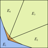
Observe that $\widehat{E}_{1}$ is not the same as $E_{1}$. Though both have the same physical boundary, they represent different regions of parametric space. Specifically, $E_{1}$ represents the entire parametric space, while $\widehat{E}_{1}$ represents only the L-shaped subset of the positive $|\boldsymbol{J}|$ region as illustrated in Fig. 6. In other words, $\widehat{E}_{1}$ corresponds to a fully invertible subset of the parametric space of the concave element.

Figure 6: (a) Parametric space. (b) $\widehat{E}_{1}$

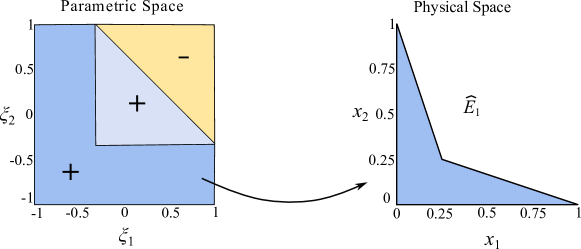
Therefore, standard Gauss quadrature cannot be employed; instead, $\widehat{E}_{1}$ is triangulated as illustrated in Fig. 7. The triangulation is used merely for the purpose of integration and does not lead to additional degrees of freedom in i-TFEM.

Figure 7: Triangulation of $\widehat{E}_{1}$

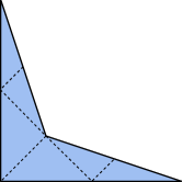
Similarly, to compute $\boldsymbol{K}_{convex}^{t}$, standard FEM procedures can be used. However, to compute $\boldsymbol{K}_{concave}^{t}$, the triangulation in Fig. 7 must be used.

3.3.2 Constraint enforcement

Finally, to compute the constraint matrix $\boldsymbol{C}$, note that the interpolation of the Lagrange multiplier $\boldsymbol{\lambda}$ needs to be only square integrable since its gradient does not appear in the formulation. For Q4 elements, the primary field $\boldsymbol{u}$ is approximated using standard bilinear functions while $\boldsymbol{N}^{\lambda}$ are constant functions. Thus, the finite dimensional approximation for the Lagrange multiplier $\boldsymbol{\lambda}$ comes from an FE space that is smaller than that for $\boldsymbol{u}$. Accordingly, we can write the constraint matrix defined in Equation 16 as

$$\boldsymbol{C}=\int\limits_{F_{1}}\left(\boldsymbol{N}_{1}^{+}-\boldsymbol{N}_{1}^{-}\right)^{\top}dV.$$ (23)

Direct integration over the tangled region $F_{1}$ to compute $\boldsymbol{C}$ is computationally expensive and cumbersome [33]. Instead, we evaluate the integrand at a sample point $\boldsymbol{x}\in F_{1}$, say the concave vertex, i.e., evaluate the $\boldsymbol{C}$ as

$$\boldsymbol{C}=\left(\boldsymbol{N}_{1}^{+}(\boldsymbol{p})-\boldsymbol{N}_{1}^{-}(\boldsymbol{p})\right)^{\top}=\llbracket\boldsymbol{N}_{1}(\boldsymbol{p})\rrbracket.$$ (24)

where $\boldsymbol{p}$ is the re-entrant vertex. Thus, the constraints can be applied directly as a set of algebraic equations. Since $\boldsymbol{u}$ is a vector field, each concave element entails two constraint equations. This is consistent, for example, with the algebraic constraints implemented in [33, 32, 31].

4 Numerical Experiments

In this section, i-TFEM is demonstrated using plane strain nonlinear elasticity problems over various tangled meshes. Numerical experiments are conducted under the following conditions:

• The implementation is in MATLAB R2022a, on a standard Windows 10 desktop with Intel(R) Core(TM) i9-9820X CPU running at 3.3 GHz with 16 GB memory.

• The number of quadrature points for convex quadrilateral elements.

• The triangulation of a concave element (see Fig. 7) is performed by employing MATLAB’s inbuilt mesher - generateMesh. The number of quadrature points for triangles is 4.

• The load is applied incrementally in 10 steps. The stopping criteria for Newton Raphson is $||\Delta\boldsymbol{{\hat{u}}}||<10^{-9}$.

Through the experiments, we investigate the following:

• Cook’s problem, single concave element: For Cook’s membrane problem [35], the error in tip displacement due to the presence of a single concave element is reported as the severity of tangling is increased.

• Cook’s problem, multiple concave elements: For Cook’s membrane problem, with numerous tangled elements: (a) The displacement at a prescribed location is reported for each load step. (b) Deformed configurations for tangled and regular meshes are also compared. (c) Convergence of the tip displacement as a function of mesh size is studied and compared against standard FEM. (d) Finally, the convergence rate is evaluated.

• Punch problem, material non-linearity: For the punch problem [37], we include material non-linearity and study the convergence characteristics of i-TFEM.

• Punch problem, multiple overlap, near-incompressibility: For the punch problem [37], a mesh with multiple overlaps is considered for compressible and near-incompressible cases.

• Thin beam problem: The performance of i-TFEM in bending dominated response is evaluated with neo-Hookean material model.

• Aircraft model: An example of a tangled mesh is presented to evaluate i-TFEM in practical scenarios.

4.1 2D Cook’s membrane: Single concave element

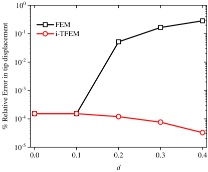
To begin with, we solve Cook’s membrane problem over the mesh with one concave element illustrated earlier in Fig. 1(b). Recall that the extent of tangling is controlled by the parameter $d$. For $d>0.1$, a sharp increase in FEM error was observed, as illustrated in Fig. 8. On the other hand, using i-TFEM, the error, in fact, decreases (slightly) for $d>0.1$; see Fig. 8.

Figure 8: Relative error in tip displacement versus $d$ for FEM and i-TFEM.

4.2 2D Cook’s membrane: Multiple concave elements

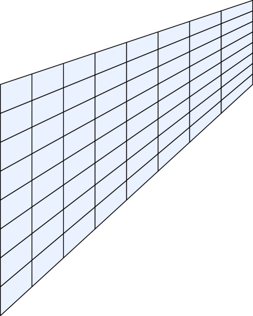
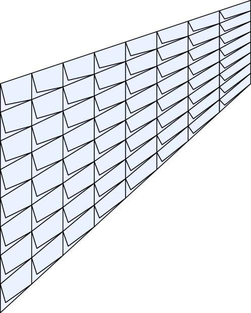
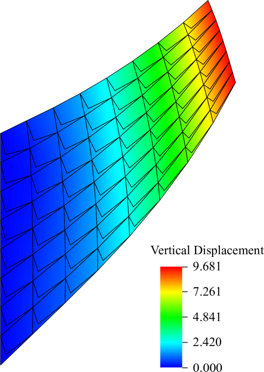
Next, we consider a regular mesh illustrated in Fig. 9(a) and a highly tangled mesh in Fig. 9(b) where every other element is concave.

(a)

(b)

Figure 9: Initial configuration for (a) Regular mesh. (b) tangled mesh with $N=3\equiv 8\times 8$ for the Cook’s membrane problem.

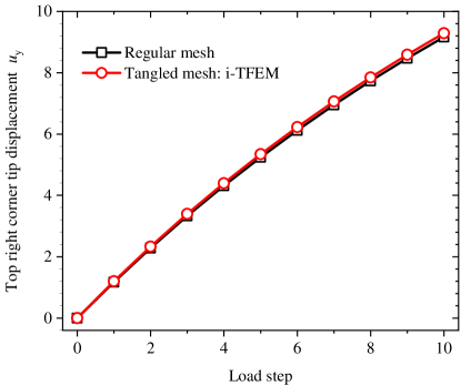
The Cook’s membrane problem is solved over the regular mesh using standard FEM, and over the tangled mesh using i-TFEM. The vertical displacement at the top right corner point A (see Fig. 1(a)) for every load step is reported in Fig. 10. One can observe a close agreement between the two.

Figure 10: Vertical displacement versus the load step for Cook’s membrane problem.

The deformed configuration for regular and tangled meshes after the last load step are reported in Fig. 11(a) and Fig. 11(b), respectively.

(a)

(b)

Figure 11: Deformed configuration for (a) Regular mesh and (b) Tangled mesh using i-TFEM for Cook’s membrane problem.

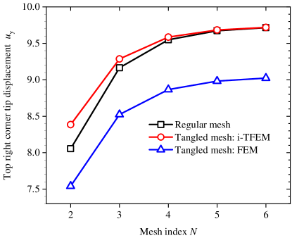
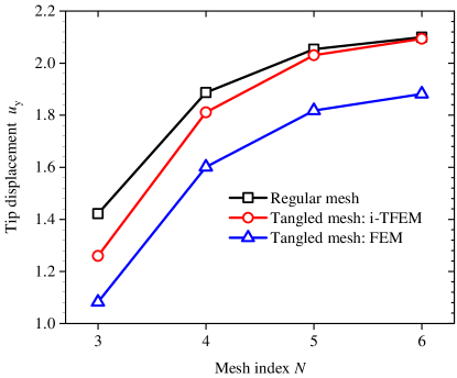
To study convergence, the number of elements is controlled by a mesh-index $N$, where the number of elements in the regular mesh is $2^{N}\times 2^{N}$. Fig. 9(a) illustrates the regular mesh when $N=3$, and Fig. 9(b), the corresponding tangled mesh. We now compare the solutions from three different methods: standard FEM over regular mesh, standard FEM over tangled mesh, and i-TFEM over tangled mesh. The vertical displacements at point A for all three are plotted as a function of $N$ in Fig. 12. Observe that FEM over a regular mesh and i-TFEM over the tangled mesh converge to the same displacement. On the other hand, FEM over a tangled mesh leads to erroneous results.

Figure 12: Convergence study for Cook’s membrane problem.

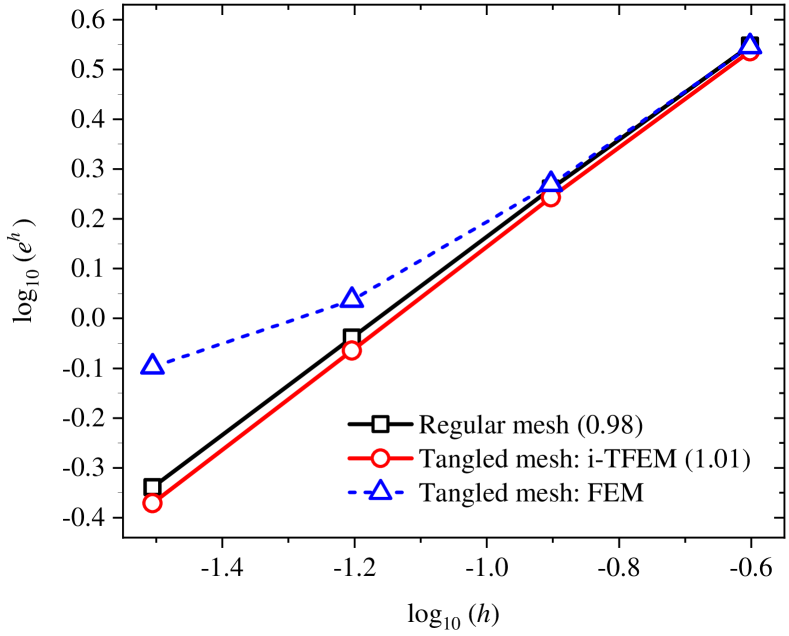
To study the rate of convergence, we define the $H^{1}$ seminorm of the displacement error as

$$e^{h}={||\nabla\boldsymbol{u}-\nabla\boldsymbol{u}^{h}||}=\left[\int\limits_{\Omega}|\nabla\boldsymbol{u}-\nabla\boldsymbol{u}^{h}|^{2}\;d\Omega\right]^{0.5}$$ (25)

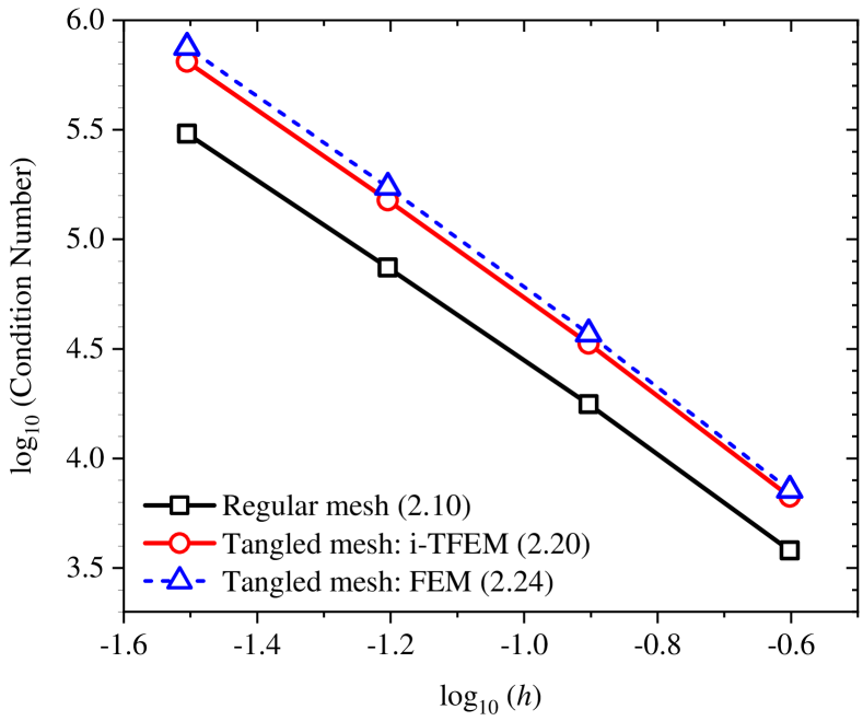
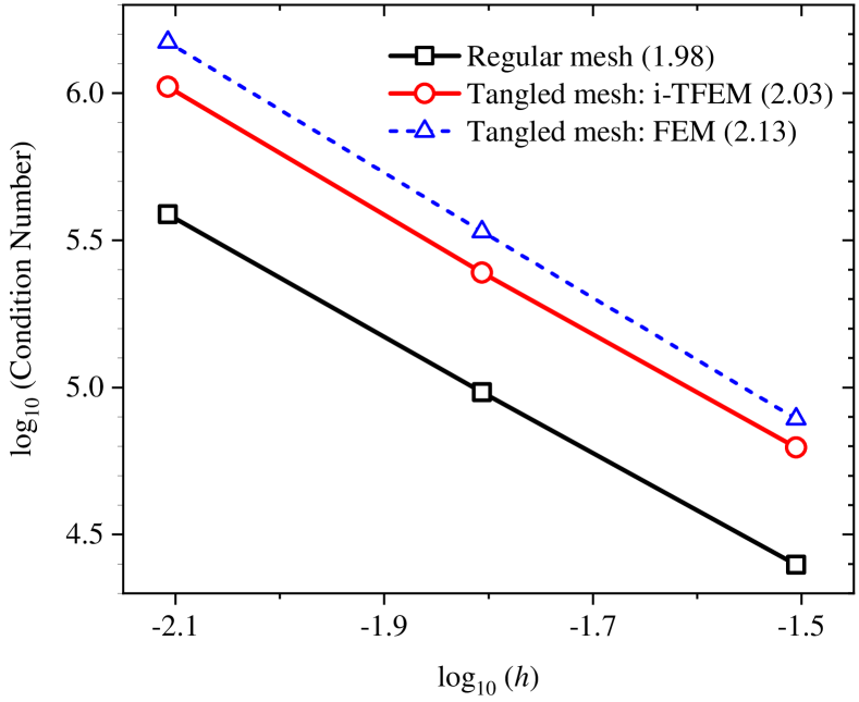
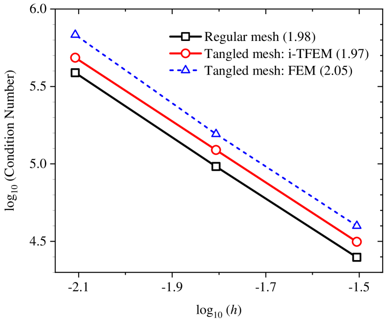
where $\boldsymbol{u}$ is the reference solution from a fine mesh with $N=7$, and $\boldsymbol{u}^{h}$ is the solution under consideration. Fig. 13(a) illustrates the error vs. mesh size ($h$) on a log-log scale over the non-tangled mesh as well as over the tangled mesh using FEM and i-TFEM. One can observe a near-optimal convergence rate for i-TFEM. Next, the effect of mesh size on the condition number of the matrix in Eq. 22 is studied. Fig. 13(b) shows that the condition number for tangled meshes increases with mesh size at a rate similar to that of a regular mesh.

(a)

(b)

Figure 13: (a)${H}^{1}$ seminorm error versus mesh size and (b) condition number versus mesh size for Cook’s problem. The convergence rates are provided in the brackets.

4.3 Punch Problem: Material nonlinearity

Next, we consider a punch problem [27, 30, 37, 28] with geometric and material nonlinearities. Specifically, compressible isotropic generalized neo-Hookean material model is considered where the strain energy density is given by [38, 39]:

$$\Psi_{\text{GNH}}\left(\boldsymbol{u}\right)=\frac{\mu}{2}\left(J_{F}^{-2/3}tr\boldsymbol{b}-3\right)+\frac{K}{2}\left(J_{F}-1\right)^{2}$$ (26)

where $J_{F}=det\boldsymbol{F}$ and $\boldsymbol{b}=\boldsymbol{F}\boldsymbol{F}^{\top}$ is the left Cauchy-Green deformation tensor while $\mu=500$ and $K=1700$ are the material parameters (equivalent to shear and bulk moduli respectively in the small strain limit). A rectangular block is subject to a vertical load $p$ (per unit length) uniformly distributed over the top left half of the block where $p=1000$ and $H=1$; see Fig. 14 [37]. The top and left sides of the block are fixed in the horizontal direction, while the bottom is fixed in the vertical direction.

Figure 14: Initial configuration of the punch problem with mesh size $N=2\equiv 8\times 4$ and the tangled mesh.

Fig. 15 captures the vertical displacement of point A (located at the top left corner) for every load step. The results for the regular mesh and tangled mesh (using i-TFEM) match well. For both meshes, the solution converged in about 5 Newton iterations for each load step.

Figure 15: Vertical displacement versus the load step for the punch problem.

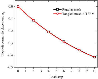
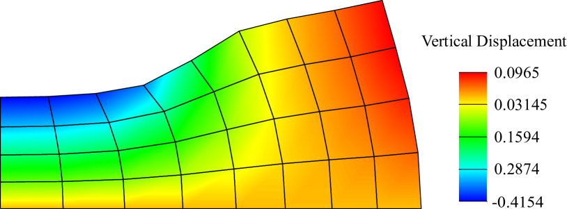
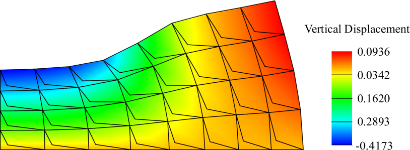
Fig. 16(a) and Fig. 16(b) illustrate the deformed configurations for the regular mesh and tangled meshes respectively, after the final load step.

(a)

(b)

Figure 16: Deformed configuration for (a) regular mesh via FEM and (b) tangled mesh via i-TFEM for the punch problem.

To study the convergence, we use the mesh index $N$ where the number of elements in the regular mesh is $2^{N+1}\times 2^{N}$. The regular and tangled meshes with $N=2$ are shown in Fig. 14. A convergence study was then carried out as $N$ was varied. The vertical displacement $u_{y}$ at point A for the two methods is plotted against the mesh index $N$ in Fig. 17. One can observe that the two methods converge to the same solution while standard FEM over the tangled mesh converges to an incorrect solution.

Figure 17: Convergence study for the punch problem.

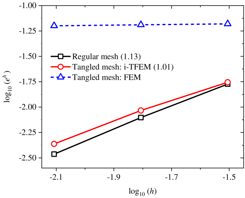
Finally, Fig. 18(a) illustrates the ${H}^{1}$ seminorm error over the tangled mesh using FEM and i-TFEM as well as over the regular mesh. The reference solution is obtained with $N=8$. Once again, i-TFEM exhibits a convergence rate for the $H^{1}$ seminorm error (Fig. 18(a)) and the condition number (Fig. 18(b)) similar to that obtained with a non-tangled mesh.

(a)

(b)

Figure 18: (a) ${H}^{1}$ seminorm error versus mesh size and (b) condition number versus mesh size for the punch problem. The convergence rates are provided in the brackets.

4.3.1 Multiple Overlaps

Thus far, the fold was shared by only one neighboring convex element. However, in practice, the fold may be shared by multiple convex elements as illustrated in Fig. 19. In this case, three convex elements $E_{2}$, $E_{3}$ and $E_{4}$ share the folded region $F_{1}$. However this does not change the methodology, i.e., the tangent matrices and constraint matrix are computed as before (1) the tangent matrix $\boldsymbol{K}_{convex}^{t}$ and residual vector $\boldsymbol{R}^{u}_{convex}$ corresponding to the convex elements are computed using the three convex elements, (2) while $\widehat{\boldsymbol{K}}_{concave}^{t}$ and $\widehat{\boldsymbol{R}}^{u}_{concave}$ are computed using the parametric space associated with $\widehat{E}_{1}$, and (3) the constraint matrix is computed using the entire fold $F_{1}$.

Figure 19: Four-element patch with one element concave.

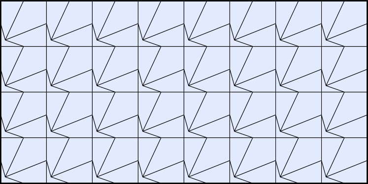
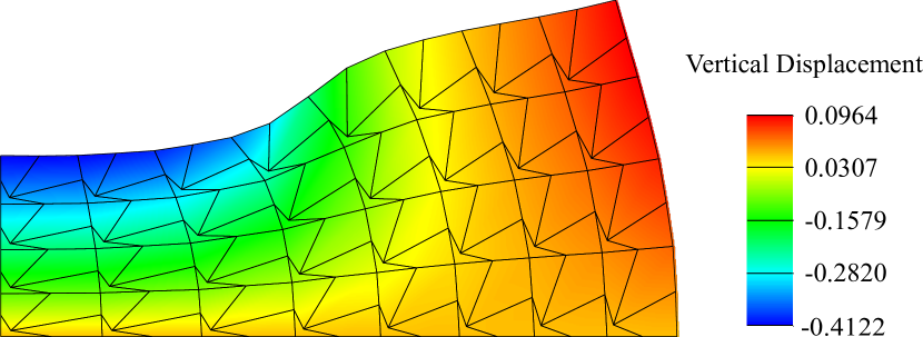
Here, we consider a tangled mesh (see Fig. 20(a)) where the basic repeating unit is the patch shown in Fig. 19. The problem described in Fig. 14 is used as a case study. The final deformed configuration obtained via i-TFEM is shown in Fig. 20(b).

(a)

(b)

Figure 20: (a) $N=3$ tangled mesh (b) Final deformed shape obtained via i-TFEM.

Next, to study the convergence, we use the mesh index $N$ where the number of elements is $2^{N+1}\times 2^{N}$. Fig. 21(a) illustrates the ${H}^{1}$ seminorm error over the tangled mesh using FEM and i-TFEM as well as over the regular mesh. The reference solution is obtained with $N=8$. Once again, i-TFEM exhibits an optimal convergence rate (Fig. 21(a)). Moreover, the condition number for i-TFEM is comparable to FEM (Fig. 21(b)).

(a)

(b)

Figure 21: (a) ${H}^{1}$ seminorm error versus mesh size and (b) condition number versus mesh size for the punch problem with the four-element patch as the repeating unit. The convergence rates are provided in the brackets.

4.3.2 Incompressibility

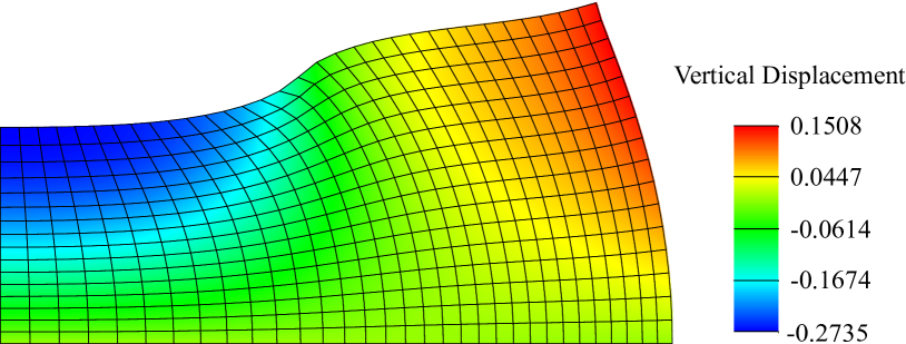
Next, we evaluate the performance of i-TFEM under near-incompressibility. Here, the F-bar method [40] is employed to prevent locking, both in FEM and i-TFEM. The punch problem (Fig. 14) is considered with the neo-Hookean material parameters $\mu=500$ and $K=5\times 10^{6}$ which results in Poisson’s ratio $\nu=0.49995$ (near-incompressibility). The problem is solved over the regular (tangle-free) mesh (shown in Fig. 14) and the tangled mesh (Fig. 20(a)). The size of the mesh is governed by the index $N$ as discussed previously. Fig. 24 shows the deformed configuration obtained over the regular mesh and via i-TFEM over tangled mesh with the mesh index $N=4$. Observe the close agreement between the two solutions.

(a)

(b)

Figure 22: Deformed configuration for (a) regular mesh via FEM and (b) tangled mesh via i-TFEM for the punch problem.

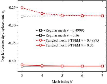
Next, we study the convergence of i-TFEM for two Poisson’s ratio values: (a) 0.49995 and (b) 0.36. Note that for Poisson’s ratio = 0.36, the F-bar method is not required. The vertical displacement $u_{y}$ at point A is plotted against the mesh index $N$ in Fig. 23 for the two methods. One can observe that i-TFEM converges to same solution as FEM in both cases.

Figure 23: Convergence study for the punch problem with the four-element patch as the repeating unit.

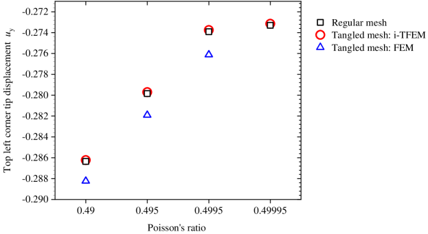
Finally, we compare the performance of FEM and i-TFEM for different Poisson’s ratios close to 0.5. For this experiement, we consider a regular mesh and a tangled mesh with $N=7$. Fig. 24 plots the vertical displacement at point A obtained by FEM and i-TFEM over tangled and untangled meshes for four values of Poisson’s ratio: 0.49, 0.495, 0.4995 and 0.49995. As opposed to FEM, the solutions obtained via i-TFEM over the tangled mesh converge to (approximately) the same value as that obtained over the untangled mesh. Note that the FEM solution over the tangled mesh at $\nu=0.49995$ is not provided since the Newton-Raphson method did not converge even with a sufficiently large number of load steps.

Figure 24: Tip vertical displacement versus different Poisson ratios for the punch problem.

4.4 Thin Beam

In this example, a beam undergoing large deflections is considered [30, 27, 37]. Specifically, a beam (see Fig. 25(a)) with a length-to-height ratio $L/H=100$ is fixed at the left end and subjected to a vertical load $F=0.1$ at the right end. The material parameters of the Neo-Hookean model (Eq. 26) are $K=16000$ and $\mu=6000$. The regular and tangled meshes are shown in Fig. 25(a) and Fig. 25(b), respectively.

(a)

(b)

Figure 25: (a) Thin beam geometry and boundary conditions with regular mesh and (b) the corresponding tangled mesh. The repeating unit for the tangled mesh is zoomed in.

The number of elements in the mesh is governed by the mesh index $N$. For the regular mesh, the number of elements in the horizontal direction is given as $(10\times 2^{N})$ while in the vertical direction, the number of elements is given by $2^{N}$ The regular mesh in Fig 23 a corresponds to $N=0$. To obtain the corresponding tangled mesh, each element is divided into a concave and a convex element. Hence the total number of elements in the tangled mesh is $2\times(10\times 2^{N})\times 2^{N}$. The final deformed configuration of the beam obtained via i-TFEM over the tangled mesh with $N=3$ is shown in Fig. 26.

Figure 26: Final deformed shape using i-TFEM with $N=3$ tangled mesh.

To study the convergence, the vertical displacement at the top right corner of the beam is considered. Fig. 27 plots the convergence of the regular mesh as well as the tangled mesh with FEM and i-TFEM. It can be seen that with i-TFEM, the solution converges to the same value as that obtained using the regular mesh.

Figure 27: Convergence study for thin beam bending problem.

4.5 Application: Aircraft model

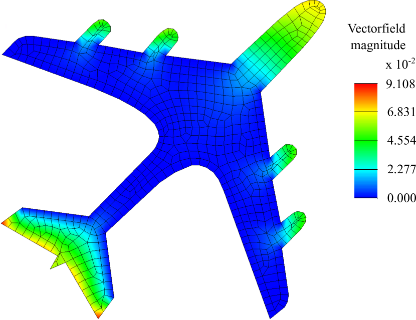
An example of a practical tangling problem is shown in Figure 28(a), where the quadrilateral mesh for an aircraft model was created using the quad mesher proposed in [41]. One quad element (out of 600) was found to be concave, for this particular model. The material parameters of the St. Venant-Kirchhoff model considered are $E=20$ and $\nu=0.3$. Symmetric (traction) boundary conditions are applied as illustrated in Fig. 28(a); the remaining boundary segments are subjected to homogenous Dirichlet boundary conditions. The problem was solved using i-TFEM and FEM. While FEM required 1.85 seconds to solve the problem, i-TFEM required 2.13 seconds.

To compare the accuracy of FEM and i-TFEM, the reference solution was obtained by solving the same problem over a very fine quadrilateral mesh with nearly 10,000 elements. The problem was then solved over the tangled quad mesh shown in Fig. 28(a) using FEM and i-TFEM. The i-TFEM solution at the re-entrant vertex had a relative error of 0.018%, while the error for FEM was 0.11%. The i-TFEM post-processed solution is illustrated in Fig. 28(b).

(a)

(b)

Figure 28: (a) Mesh for an aircraft model, with one concave element. (b) i-TFEM solution.

5 Conclusions

It is well-known that concave elements lead to a non-invertible parametric mapping which, in turn, leads to erroneous solutions in standard FEM. To resolve this, an isoparametric tangled finite element method (i-TFEM) was proposed for nonlinear elasticity with material nonlinearity, over bi-linear quadrilateral meshes.

The proposed method replaces the full-invertibility requirement with the partial invertibility by incorporating compatibility constraints, thereby allowing for tangled (concave) elements to be present in the mesh. The constraints are imposed via Lagrange multipliers, and the corresponding mixed variational formulation was presented. Moreover, the proposed definition of the field in the tangled region naturally leads to modification in the elemental stiffness matrices over the concave elements.

Numerical simulations reproducing a set of well-known benchmark tests are promising. i-TFEM converges to the expected solution even in the presence of severely tangled elements. Moreover, the convergence rate and condition number of i-TFEM are comparable over tangled meshes with that of the standard FEM over non-tangled meshes.

The proposed method can potentially be extended to three dimensions and isogeometric analysis where tangling is known to occur [42, 43].

References

- [1] O. C. Zienkiewicz, R. L. Taylor, J. Z. Zhu, The finite element method: its basis and fundamentals, Elsevier, 2005.
- [2] P. J. Frey, P.-L. George, Mesh generation: application to finite elements, Iste, 2007.
- [3] R. D. Cook, et al., Concepts and applications of finite element analysis, John wiley & sons, 2007.
- [4] D. S. Lo, Finite element mesh generation, CRC Press, 2014.
- [5] T. Blacker, Automated conformal hexahedral meshing constraints, challenges and opportunities, Engineering with Computers 17 (3) (2001) 201–210.
- [6] N. Pietroni, M. Campen, A. Sheffer, G. Cherchi, D. Bommes, X. Gao, R. Scateni, F. Ledoux, J.-F. Remacle, M. Livesu, Hex-mesh generation and processing: a survey, ACM Transactions on Graphics (TOG) (2022).
- [7] M. Mandad, R. Chen, D. Bommes, M. Campen, Intrinsic mixed-integer polycubes for hexahedral meshing, Computer Aided Geometric Design 94 (2022) 102078.
- [8] X. Fang, W. Xu, H. Bao, J. Huang, All-hex meshing using closed-form induced polycube, ACM Transactions on Graphics (TOG) 35 (4) (2016) 1–9.
- [9] M. Livesu, N. Vining, A. Sheffer, J. Gregson, R. Scateni, Polycut: Monotone graph-cuts for polycube base-complex construction, ACM Transactions on Graphics (TOG) 32 (6) (2013) 1–12.
- [10] J. Gregson, A. Sheffer, E. Zhang, All-hex mesh generation via volumetric polycube deformation, in: Computer graphics forum, Vol. 30, Wiley Online Library, 2011, pp. 1407–1416.
- [11] T. Jiang, J. Huang, Y. Wang, Y. Tong, H. Bao, Frame field singularity correctionfor automatic hexahedralization, IEEE Transactions on Visualization and Computer Graphics 20 (8) (2013) 1189–1199.
- [12] Y. Li, Y. Liu, W. Xu, W. Wang, B. Guo, All-hex meshing using singularity-restricted field, ACM Transactions on Graphics (TOG) 31 (6) (2012) 1–11.
- [13] M. Nieser, U. Reitebuch, K. Polthier, Cubecover–parameterization of 3d volumes, in: Computer graphics forum, Vol. 30, Wiley Online Library, 2011, pp. 1397–1406.
- [14] J. Huang, Y. Tong, H. Wei, H. Bao, Boundary aligned smooth 3d cross-frame field, ACM transactions on graphics (TOG) 30 (6) (2011) 1–8.
- [15] M. Livesu, A. Sheffer, N. Vining, M. Tarini, Practical hex-mesh optimization via edge-cone rectification, ACM Transactions on Graphics (TOG) 34 (4) (2015) 1–11.
- [16] K. Xu, X. Gao, G. Chen, Hexahedral mesh quality improvement via edge-angle optimization, Computers & Graphics 70 (2018) 17–27.
- [17] P. M. Knupp, Hexahedral and tetrahedral mesh untangling, Engineering with Computers 17 (3) (2001) 261–268.
- [18] E. Ruiz-Gironés, X. Roca, J. Sarrate, R. Montenegro, J. M. Escobar, Simultaneous untangling and smoothing of quadrilateral and hexahedral meshes using an object-oriented framework, Advances in Engineering Software 80 (2015) 12–24.
- [19] Q. Huang, W.-X. Zhang, Q. Wang, L. Liu, X.-M. Fu, Untangling all-hex meshes via adaptive boundary optimization, Graphical Models 121 (2022) 101136.
- [20] M. N. Akram, L. Si, G. Chen, An embedded polygon strategy for quality improvement of 2d quadrilateral meshes with boundaries., in: VISIGRAPP (1: GRAPP), 2021, pp. 177–184.
- [21] G. Liu, K. Dai, T. T. Nguyen, A smoothed finite element method for mechanics problems, Computational Mechanics 39 (6) (2007) 859–877.
- [22] N. Sukumar, A. Tabarraei, Conforming polygonal finite elements, International Journal for Numerical Methods in Engineering 61 (12) (2004) 2045–2066.
- [23] L. Beirão da Veiga, F. Brezzi, A. Cangiani, G. Manzini, L. D. Marini, A. Russo, Basic principles of virtual element methods, Mathematical Models and Methods in Applied Sciences 23 (01) (2013) 199–214.
- [24] S. Cen, P.-L. Zhou, C.-F. Li, C.-J. Wu, An unsymmetric 4-node, 8-dof plane membrane element perfectly breaking through macneal’s theorem, International Journal for Numerical Methods in Engineering 103 (7) (2015) 469–500.
- [25] H. Chi, C. Talischi, O. Lopez-Pamies, G. H. Paulino, Polygonal finite elements for finite elasticity, International Journal for Numerical Methods in Engineering 101 (4) (2015) 305–328.
- [26] J. E. Bishop, N. Sukumar, Polyhedral finite elements for nonlinear solid mechanics using tetrahedral subdivisions and dual-cell aggregation, Computer Aided Geometric Design 77 (2020) 101812.
- [27] P. Wriggers, B. Reddy, W. Rust, B. Hudobivnik, Efficient virtual element formulations for compressible and incompressible finite deformations, Computational Mechanics 60 (2017) 253–268.
- [28] D. van Huyssteen, B. D. Reddy, A virtual element method for isotropic hyperelasticity, Computer Methods in Applied Mechanics and Engineering 367 (2020) 113134.
- [29] H. Chi, L. B. Da Veiga, G. Paulino, Some basic formulations of the virtual element method (vem) for finite deformations, Computer Methods in Applied Mechanics and Engineering 318 (2017) 148–192.
- [30] Z. Li, S. Cen, J. Huang, C.-F. Li, Hyperelastic finite deformation analysis with the unsymmetric finite element method containing homogeneous solutions of linear elasticity, International Journal for Numerical Methods in Engineering 121 (16) (2020) 3702–3721.
- [31] B. Prabhune, K. Suresh, A computationally efficient isoparametric tangled finite element method for handling inverted quadrilateral and hexahedral elements, Computer Methods in Applied Mechanics and Engineering 405 (2023) 115897.
- [32] B. Prabhune, K. Suresh, Towards tangled finite element analysis over partially inverted hexahedral elements, arXiv preprint arXiv:2207.03905 (2022).
- [33] B. Prabhune, S. Sridhara, K. Suresh, Tangled finite element method for handling concave elements in quadrilateral meshes, International Journal for Numerical Methods in Engineering 123 (7) (2022) 1576–1605.
- [34] J. N. Reddy, An Introduction to Nonlinear Finite Element Analysis Second Edition: with applications to heat transfer, fluid mechanics, and solid mechanics, OUP Oxford, 2014.
- [35] R. D. Cook, Improved two-dimensional finite element, Journal of the Structural Division 100 (9) (1974) 1851–1863.
- [36] J. Danczyk, K. Suresh, Finite element analysis over tangled simplicial meshes: Theory and implementation, Finite Elements in Analysis and Design 70 (2013) 57–67.
- [37] M. De Bellis, P. Wriggers, B. Hudobivnik, Serendipity virtual element formulation for nonlinear elasticity, Computers & Structures 223 (2019) 106094.
- [38] O. C. Zienkiewicz, R. L. Taylor, R. L. Taylor, The finite element method: solid mechanics, Vol. 2, Butterworth-heinemann, 2000.
- [39] A. F. Bower, Applied mechanics of solids, CRC press, 2009.
- [40] E. D. S. Neto, F. A. Pires, D. Owen, F-bar-based linear triangles and tetrahedra for finite strain analysis of nearly incompressible solids. part i: formulation and benchmarking, International Journal for Numerical Methods in Engineering 62 (3) (2005) 353–383.
- [41] J. Sarrate, A. Huerta, Efficient unstructured quadrilateral mesh generation, International journal for numerical methods in engineering 49 (10) (2000) 1327–1350.
- [42] D. Fußeder, B. Simeon, A.-V. Vuong, Fundamental aspects of shape optimization in the context of isogeometric analysis, Computer Methods in Applied Mechanics and Engineering 286 (2015) 313–331.
- [43] S. Xia, X. Qian, Generating high-quality high-order parameterization for isogeometric analysis on triangulations, Computer Methods in Applied Mechanics and Engineering 338 (2018) 1–26.