Uncertainty Driven Bottleneck Attention U-net for OAR Segmentation

Abstract

Organ at risk (OAR) segmentation in computed tomography (CT) imagery is a difficult task for automated segmentation methods and can be crucial for downstream radiation treatment planning. U-net has become a de-facto standard for medical image segmentation and is frequently used as a common baseline in medical image segmentation tasks. In this paper, we develop a multiple decoder U-net architecture where a noisy auxiliary decoder is used to generate noisy segmentation. The segmentation from the main branch and the noisy segmentation from the auxiliary branch are used together to estimate the attention. Our contribution is the development of a new attention module which derives the attention from the softmax probabilities of two decoder branches. The union and intersection of two segmentation masks from two branches carry the information where both decoders agree and disagree. The softmax probabilities from regions of agreement and disagreement are the indicators of low and high uncertainty. Thus, the probabilities of those selected regions are used as attention in the bottleneck layer of the encoder and passes only through the main decoder for segmentation. For accurate contour segmentation, we also developed a CT intensity integrated regularization loss. We tested our model on two publicly available OAR challenge datasets, Segthor and LCTSC respectively. We trained 12 models on each dataset with and without the proposed attention model and regularization loss to check the effectiveness of the attention module and the regularization loss. The experiments demonstrate a clear accuracy improvement (2% to 5% Dice) on both datasets. Code for the experiments will be made available upon the acceptance for publication.

horacic CT, Organs-at-Risk, Uncertainty, U-net.

1 Introduction

Radiation treatment planing requires meticulous delineation of organs that are adjacent to affected tissues. Delineating organs at risk (OAR) is tedious, time consuming and prone to inter-rater variability leading to unnecessary and dangerous radiation to healthy tissues. Recently, deep learning based methods have achieved remarkable success in image segmentation for both natural and medical images. Many deep learning-based methods have been developed to simultaneously segment multiple organs. Segmenting multiple organs is a challenging task due to the variation of the organ shape, the low soft tissue contrast in CT and label imbalance. Deep learning models are particularly good at segmenting when organs are relatively large, consistent in shape and their boundary tissues have a high contrast compared to background organs/structures. In the case of smaller organs, models struggle to segment them effectively and sometimes, segmentation completely fails to detect the organ. In chest CT scans, the esophagus is the most challenging organ [2] to segment due to its high shape variation and low soft tissue contrast.

U-net become a standard model for medical image segmentation[11]. Many different variants of the U-net model have been developed in recent years [15, 5, 4, 8, 14, 13]. Most of these works have concentrated their effort in adding more layers or aggregating robust context information while processing the image in the layers of the U-net. In [9], an attention gate is proposed for U-net, where the attention distribution is generated by processing the features from the deeper layer and shallower layers. Sinha et.al [12] proposed guided multi resolution attention where attention is generated by aggregating multi-resolution features and is guided by a deep supervision loss. Similar deep feature based works also include [3],[7] and [17] where authors proposed different attention mechanisms. Despite their high accuracy, adding attention module/gates adds extra layers of complexity. Since neural networks learn to extract optimal features during training, adding attention gates places additional burden on the network to find optimal attention parameters in an unexplainable way. As such, the parameter search space increases exponentially with the added attention type (spatial,channel,recurrent etc).

To address these issues, this paper proposes two contributions. First, the use of an auxiliary decoder in the U-net architecture allows for the extraction of uncertainties between the main and auxiliary segmentation, which can be used as attention. This approach generates attention that is more explainable and easier to manipulate. Second, to address the inherent complexity of segmenting very close organs, a CT intensity integrated regularization method is proposed, which is tested on two OAR segmentation datasets.

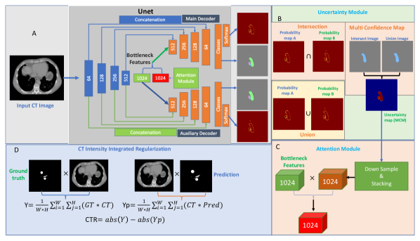
Figure 1: Overview of the proposed approach.A) The U-net with auxiliary decoder. B) The Uncertainty module, C) Attention module, D)CT intensity integrated regularization.

2 Method

The proposed method is depicted in Figure 1. The approach utilizes a U-net architecture with two decoders. The main decoder sequentially processes bottleneck features, along with skip connections, to produce the segmentation output. Instead of directly using the bottleneck features from the encoder, in auxiliary decoder, a perturbation layer is introduced, similar to the approach presented in [10]. The perturbation layer employs random noise with a uniform distribution of $U(-0.3,0.3)$ to modify the auxiliary decoder’s output. The segmentation outputs from both decoders are then used in the uncertainty module, which applies union and intersection operations to generate the corresponding masks. This module’s concept is derived from [1], but instead of using ground-truth segmentation from multiple radiologists, the uncertainty is estimated from the agreement and disagreement of the two decoders. The union mask takes all regions where both decoders agree and disagree, while the intersection mask takes only the regions where they agree. Similar to [1], combining the intersection and union masks provides the multi-confidence mask (MCM) (see Figure 1(B)). To extract the probabilities from the regions in the MCM, the maximum of the softmax function is applied to the output of each decoder, and the resulting values are multiplied with the multi-confidence mask. The equations for this procedure are as follows:

$$p_{main}=max(softmax(D_{main},dim=1))$$ (1)

$$p_{aux}=max(softmax(D_{aux},dim=1))$$ (2)

$$Attention=max(p_{main},p_{aux})*MCM$$ (3)

Here, $D_{main}$ and $D_{aux}$ are the $1\times 1$ regression layer output from main and auxiliary decoders. The calculated attention is a single channel spatial attention where the probabilities of each pixel is obtained from the region of interest. To apply this attention to the bottleneck features, the spatial dimensions are downsampled and replicated along the channel dimension to match with dimension of the bottleneck. Finally, the attention is multiplied with the bottleneck features to select features that are required for the segmentation (see Figure1(C)).

Dice and cross entropy losses are commonly employed in medical image segmentation. The dice loss evaluates the agreement between the predicted segmentation and the actual segmentation. Thus, it primarily takes into account the shape of the object of interest. In contrast, the cross-entropy loss relies heavily on the distribution of the classes in the dataset. If the classes are evenly distributed, the classification results will be better. Since OAR segmentation requires precise boundary segmentation, the use of mere shape or class distribution sometime classify surrounding the boundary pixels as false positive. Based on this observation, we introduce ct-intensity integrated regularization (CTR).In CTR (shown in Figure1(D)), the CT intensities from the ground-truth and predicted regions are extracted using corresponding masks and absolute differences are measured. Thus, the calculated CTR helps the network learn CT intensity distributions more accurately. We also proposed a matrix version of CTR which compares both the intra-class and inter-class CT intensities.
Let consider, $Y$ and $Y_{p}$ are the CT-intensities extracted from the the predicted and ground-truth regions and given by:

$$Y=\frac{1}{WH}\sum_{i=1}^{W}\sum_{j=1}^{H}CT*GT_{mask}$$ (4)

$$Y_{p}=\frac{1}{WH}\sum_{i=1}^{W}\sum_{j=1}^{H}CT*P_{mask}$$ (5)

Therefore, the CT-intensity-integrated regularizer is

$$\mathcal{L_{CTR}}=||Y-Y_{p}||$$ (6)

Let the number of classes are $\mathcal{N}$, the matrix version of CTR is a $\mathcal{N}\times\mathcal{N}$ matrix which is given by:

$$\mathcal{M_{CTR}}=[\mathcal{CTR}_{i,j}]$$ (7)

Each entry of the matrix is the CTR value between i-th class ground-truth and j-th class prediction, therefore inter-class CTR. When $i=j$ its the intra-class CTR. For simplicity we denote CTR matrix as CTRM. To optimize the network, the mean of the CTRM is taken and the resulting regularizer is given by

$$\mathcal{L_{CTRM}}=\frac{1}{\mathcal{N}\mathcal{N}}\sum_{i=1}^{\mathcal{N}}\sum_{j=1}^{\mathcal{N}}[\mathcal{CTR}_{i,j}]$$ (8)

The proposed network has two segmentation decoders with slightly different segmentation outputs. Driving both decoders simultaneously require strong gradient computation and also need to maintain consistency between the segmentation outputs mentioned in [10]. We train the network with four losses, two for segmentation, one for cross-consistency between the decoders and the last one is the either of the regularizer mentioned in Eq.6 and 7. Therefore, the training loss is

$$\mathcal{L}=\mathcal{L}_{main}+\mathcal{L}_{aux}+\mathcal{L}_{CCT}+\mathcal{L_{CTR}}or\mathcal{L_{CTRM}}$$ (9)

3 Experiments and Results

3.1 Dataset and Implementation

The proposed regularization losses and attention module are evaluated on two datasets, namely SegThor [6] and LCTSC [16]. The SegThor challenge dataset consists of 40 CT images for training and 20 for testing. Unfortunately, we were only able to collect the training dataset, which includes 40 CT images along with corresponding manual annotations of the Esophagus, Heart, Trachea, and Aorta. Since only training set is available, we split the dataset with 35 for training and 5 for testing. On the other hand, the LCTSC dataset [16] comprises 36 training and 24 testing CT images with corresponding manual annotations of organs such as the Esophagus, Spinal Cord, Heart, Left and Right Lung.

The model is implemented using PyTorch version 1.12.1 as a 2D model, considering only the axial view of the 3D CT image during training. All the models are trained and tested in a high-performance computing environment with a 64GB RAM, A100 GPU, and a single-core 2.66GHz 64-bit Intel Xeon processor. The network is trained using the ADAM optimizer with a learning rate of 0.01 and batch size of 1 for 200 training epochs.

3.2 Data Preprocessing

The same data pre-processing pipeline is applied to both datasets. Specifically, 2D axial slices are extracted from each 3D volume by selecting only the body region. To enhance contrast, a level of 30 and window of 400 of the CT intensities are applied. To facilitate the evaluation of models and fit the data into the GPU memory, the image slices of size $512\times 512$ are resized to $256\times 256$. The evaluation of the proposed model was primarily based on the Dice coefficient and its standard deviation. Additionally, average surface distance (ASD) and intersection over union (IoU) are also employed for performance comparison between the proposed model and a baseline model.

3.3 Experiment Design

Twelve different experiments are conducted on each dataset. Each loss/loss-combination is tested with and without attention. In Table-1 and Table-3 the first column indicates the loss functions, rest columns are the mean dice $\pm$ standard deviation for each organ. The best performance for each organ is highlighted in bold. The UDBA suffix indicates the use of proposed attention module.

3.4 Results on SegThor Dataset

Table 1 reports the dice accuracy of U-nets on the SegThor dataset for four organs - Esophagus, Heart, Trachea, and Aorta. It is clear from the Table-1 data, that the different loss combination performs differently on four different organs. For esophagus, the model with dice and UDBA achieves the top score with 0.81$\pm$0.045. For heart, the cross-entropy and its combinations are in leading position compared to the dice losses. The CE with attention and CE+CTRM with attention achieves the 0.95$\pm$0.008 and 0.95$\pm$0.007 for the heart. Same pattern goes for the trachea, the CE and its combinations are achieving higher dice scores compared to the dice variants. Again, in the trachea, the CE+CTRM with attention achieves the top dice score with 0.91$\pm$0.022. In aorta, the dice scores of dice loss variants fluctuates between 0.90 to 0.92 while the cross-entropy variants are fluctuating from 0.89 to 0.93. Again, in aorta the CE+CTRM(UDBA) scores the highest dice score with 0.93$\pm 0.013$. Additionally, the most significant pattern we find from the Table-1 is the influence of UDBA module on the performance scores. In most of the cases the use of UDBA module systematically improves the accuracy regardless of loss combinations.

The performance of the proposed model in comparison to another attention based model is reported in Table-2. In addition to dice, average surface distance (ASD) and intersection over union (IoU) metrics are also added. To compare, we considered our Dice(UDBA) and CE+CTRM(UDBA) methods since both achieve high scores in different organs. The Dice(UDBA) method achieves the highest Dice scores for the esophagus, as well as the lowest ASD score for the trachea structure. In terms of IoU, both CE+CTRM(UDBA) and AttUnet scores higher than the Dice(UDBA). For heart, CE+CTRM(UDBA) obtains top scores in all three metrics. In trachea and aorta, this method achieves best accuracy in terms of dice and IoU metrics. The AttUnet[9] achieves lower scores in general than ours with the exception of the ASD, IoU in esophagus, and ASD in Aorta. Since we do not have SegThor test dataset, we are unable to compare side-by-side with methods presented in the challenge ledger board.

Table 1: Dice Accuracy of Unets with and without attention module on Segthor Dataset. Combination of different losses and proposed regularizations are also presented.

Losses (Unet) Esophagus Heart Trachea Aorta Dice $0.74\pm 0.060$ $0.93\pm 0.009$ $0.85\pm 0.025$ $0.91\pm 0.015$ Dice(UDBA) $\textbf{0.81}\pm 0.045$ $0.93\pm 0.021$ $0.84\pm 0.033$ $0.92\pm 0.012$ Dice+CTR $0.72\pm 0.067$ $0.92\pm 0.010$ $0.84\pm 0.023$ $0.90\pm 0.028$ Dice+CTR(UDBA) $0.76\pm 0.082$ $0.93\pm 0.019$ $0.87\pm 0.035$ $0.92\pm 0.013$ Dice+CTRM $0.75\pm 0.079$ $0.93\pm 0.017$ $0.84\pm 0.038$ $0.90\pm 0.027$ Dice+CTRM(UDBA) $0.74\pm 0.058$ $0.93\pm 0.016$ $0.87\pm 0.021$ $0.92\pm 0.013$ CE $0.71\pm 0.068$ $0.94\pm 0.011$ $0.88\pm 0.035$ $0.89\pm 0.028$ CE(UDBA) $0.78\pm 0.052$ $\textbf{0.95}\pm 0.008$ $0.90\pm 0.032$ $0.92\pm 0.018$ CE+CTR $0.70\pm 0.129$ $0.93\pm 0.015$ $0.89\pm 0.025$ $0.88\pm 0.042$ CE+CTR(UDBA) $0.74\pm 0.082$ $0.94\pm 0.013$ $0.90\pm 0.015$ $0.92\pm 0.016$ CE+CTRM $0.69\pm 0.094$ $0.93\pm 0.014$ $0.88\pm 0.031$ $0.86\pm 0.027$ CE+CTRM(UBDA) $0.74\pm 0.092$ $\textbf{0.95}\pm 0.007$ $\textbf{0.91}\pm 0.022$ $\textbf{0.93}\pm 0.013$

Table 2: Comparison between other baselines on SegThor Dataset

Method Esophagus Heart Trachea Aorta Dice ASD IoU Dice ASD IoU Dice ASD IoU Dice ASD IoU Dice(UDBA) 0.81 0.82 0.87 0.92 1.11 0.78 0.85 0.46 0.84 0.92 0.73 0.91 CE+CTRM(UDBA) 0.74 1.45 0.89 0.95 0.94 0.93 0.91 0.57 0.95 0.93 0.66 0.93 AttUnet[9] 0.74 0.66 0.89 0.80 1.57 0.61 0.80 0.50 0.86 0.88 0.59 0.88

3.5 Results on LCTSC Dataset

The Table-3 presents the dice accuracy of U-nets with and without an attention module on the LCTSC dataset. The dataset has five different regions of interest, including Esophagus, Spinal Cord, Heart, left and right Lung. In Table-3, Dice with CTRM and UDBA achieves the top score for esophagus and spinal cord with dice 0.71$\pm$0.063 and 0.89$\pm$0.009, respectively. For heart and both lungs, the cross-entropy with UDBA achieves the highest scores in all three regions with the scores 0.92$\pm$0.033, 0.97$\pm$0.003 and 0.97$\pm$0.003. The combination CE+CTRM(UDBA) also achieves very similar scores to CE(UDBA) in four organs except the esophagus.
In this Table-3, dice based models are consistently achieved high scores in esophagus and spinal cord compared to their cross-entropy based counterparts. For other three organs, cross-entropy based combinations are performed better than the dice based combinations. Similar to Table-1, the use of UDBA module consistently improves the accuracy regardless of loss combinations.

Table 3: Dice Accuracy of Unets with and without attention module on LCTSC Dataset. Combination of different losses and proposed regularization are also presented.

Losses (Unet) Esophagus Spine Heart Lung(Left) Lung(Right) Dice $0.66\pm 0.019$ $0.88\pm 0.031$ $0.71\pm 0.092$ $0.94\pm 0.043$ $0.95\pm 0.042$ Dice(UDBA) $0.68\pm 0.085$ $0.88\pm 0.026$ $0.82\pm 0.034$ $0.96\pm 0.017$ $0.95\pm 0.030$ Dice+CTR $0.63\pm 0.097$ $0.88\pm 0.030$ $0.81\pm 0.039$ $0.93\pm 0.045$ $0.95\pm 0.038$ Dice+CTR(UDBA) $0.68\pm 0.096$ $0.88\pm 0.027$ $0.47\pm 0.070$ $0.93\pm 0.046$ $0.94\pm 0.053$ Dice+CTRM $0.65\pm 0.052$ $0.88\pm 0.009$ $0.78\pm 0.05$ $0.93\pm 0.013$ $0.94\pm 0.004$ Dice+CTRM(UDBA) $\textbf{0.71}\pm 0.063$ $\textbf{0.89}\pm 0.009$ $0.88\pm 0.029$ $0.95\pm 0.002$ $0.96\pm 0.002$ CE $0.61\pm 0.038$ $0.86\pm 0.011$ $0.89\pm 0.042$ $0.96\pm 0.005$ $0.96\pm 0.004$ CE(UDBA) $0.63\pm 0.044$ $0.88\pm 0.012$ $\textbf{0.92}\pm 0.033$ $\textbf{0.97}\pm 0.003$ $\textbf{0.97}\pm 0.003$ CE+CTR $0.56\pm 0.111$ $0.86\pm 0.030$ $0.90\pm 0.038$ $0.96\pm 0.017$ $0.96\pm 0.021$ CE+CTR(UDBA) $0.62\pm 0.100$ $0.87\pm 0.033$ $0.91\pm 0.037$ $0.96\pm 0.015$ $0.97\pm 0.021$ CE+CTRM $0.52\pm 0.134$ $0.86\pm 0.026$ $0.90\pm 0.033$ $0.96\pm 0.018$ $0.96\pm 0.022$ CE+CTRM(UDBA) $0.63\pm 0.082$ $0.88\pm 0.025$ $\textbf{0.92}\pm 0.024$ $0.96\pm 0.016$ $0.97\pm 0.022$

Similar to SegThor data, we compare the performance of two of our models with the attention U-net[9]. Table 4 presenting the comparison data using Dice,ASD and IoU. The models we chose are from best performing dice based model and the best performing cross-entropy based model. In this table, the CE+CTRM(UDBA) method achieves the best performance on four out of five organs (Esophagus, Spine, Heart, and Lung(R)) in terms of Dice, and on all five organs in terms of IoU. The Dice+CTRM(UDBA) method performs the best on esophagus and spine in terms of Dice coefficient, but not performing well on other three organs. The AttUnet method performs better on Esophagus in terms of ASD, but not as well as CE+CTRM(UDBA) and Dice+CTRM(UDBA) in terms of Dice coefficient and IoU. Overall, CE+CTRM(UDBA) appears to be the best performing method based on the evaluation metrics used in this table. For LCTSC dataset, the challenge organizers kept the ledger board private. Hence we are unable to compare side-by-side with the other baseline methods.

Table 4: Comparison between other baselines on LCTSC Dataset

Method Esophagus Spine Heart Lung(L) Lung(R) Dice ASD IoU Dice ASD IoU Dice ASD IoU Dice ASD IoU Dice ASD IoU CE+CTRM(UDBA) 0.63 1.76 0.80 0.88 0.71 0.91 0.92 1.35 0.84 0.97 0.65 0.92 0.97 0.71 0.92 Dice+CTRM(UDBA) 0.71 1.58 0.75 0.89 0.66 0.89 0.88 1.78 0.50 0.95 0.62 0.85 0.96 0.68 0.89 AttUnet[9] 0.66 1.09 0.70 0.89 0.66 0.91 0.69 3.26 0.39 0.95 0.68 0.86 0.96 0.72 0.90

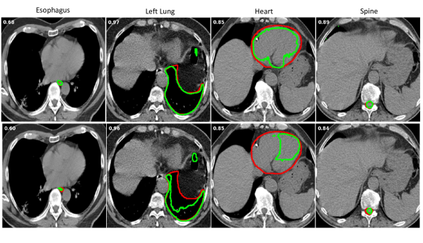
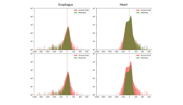
(a) Segmentations on SegThor dataset. (b) Segmentations on LCTSC dataset.

(c) 3D CT intensity distribution overlap (Frequencies are in log scale)

Figure 2: In (a) and (b), top rows are the results from the methods with attention and the bottom rows are from same methods without attention. Red and Green color represents ground-truth and predictions respectively. (c) The intensity histogram overlap of ground-truth and predictions from the Esophagus and Heart regions.Similar to (a) and (b), the top row is from methods with attention and bottom row is without attention methods.

4 Discussion and Conclusion

In this work, we presented the utilization of slightly different network segmentation outputs to estimate uncertainty. We also demonstrated that estimated uncertainty can function as attention to enhance segmentation accuracy. Our team created a simple, easy-to-implement 2D U-net architecture that was trained exclusively with axial views. The application of uncertainty-based attention for improved segmentation was validated through experiments on two OAR segmentation datasets. Figure 2 (a) and (b) showcase 2D segmentation outputs using methods with and without attention, respectively. Additionally, 3D CT intensity histogram overlap (c) was presented to provide a more comprehensive view of segmentation accuracy. This histogram further highlights the effectiveness of the proposed attention module.

We also introduced the CT intensity integrated regularization loss to help the network learn texture distributions of organs and their shapes. Experimental evaluation confirmed efficiency of intensity integration for difficult-to-segment organs. Future research will focus on further improving the accuracy of proposed regularizer near the boundary of closely located organs.

4.0.1 Acknowledgment

The authors declare no conflict of interest. Technically, the work is heavily supported by QUT High Performance Computing (HPC) facility.

References

- [1] Chen, X., Sun, S., Bai, N., Han, K., Liu, Q., Yao, S., Tang, H., Zhang, C., Lu, Z., Huang, Q., et al.: A deep learning-based auto-segmentation system for organs-at-risk on whole-body computed tomography images for radiation therapy. Radiotherapy and Oncology 160, 175–184 (2021)
- [2] Fechter, T., Adebahr, S., Baltas, D., Ben Ayed, I., Desrosiers, C., Dolz, J.: Esophagus segmentation in CT via 3D fully convolutional neural network and random walk. Medical Physics 44(12), 6341–6352 (Oct 2017)
- [3] Gu, R., Wang, G., Song, T., Huang, R., Aertsen, M., Deprest, J., Ourselin, S., Vercauteren, T., Zhang, S.: Ca-net: Comprehensive attention convolutional neural networks for explainable medical image segmentation. IEEE Transactions on Medical Imaging 40(2), 699–711 (2021)
- [4] Heinrich, M.P., Oktay, O., Bouteldja, N.: Obelisk-net: Fewer layers to solve 3d multi-organ segmentation with sparse deformable convolutions. Medical Image Analysis 54, 1–9 (2019)
- [5] Kakeya, H., Okada, T., Oshiro, Y.: 3d u-japa-net: Mixture of convolutional networks for abdominal multi-organ ct segmentation. In: Frangi, A.F., Schnabel, J.A., Davatzikos, C., Alberola-López, C., Fichtinger, G. (eds.) MICCAI 2018. pp. 426–433 (2018)
- [6] Lambert, Z., Petitjean, C., Dubray, B., Ruan, S.: Segthor: Segmentation of thoracic organs at risk in ct images (2019), https://arxiv.org/abs/1912.05950
- [7] Li, Y., Yang, J., Ni, J., Elazab, A., Wu, J.: Ta-net: Triple attention network for medical image segmentation. Computers in Biology and Medicine 137 (2021)
- [8] Milletari, F., Navab, N., Ahmadi, S.A.: V-net: Fully convolutional neural networks for volumetric medical image segmentation. In: 2016 Fourth International Conference on 3D Vision (3DV). pp. 565–571 (2016)
- [9] Oktay, O., Schlemper, J., Folgoc, L.L., Lee, M.C.H., Heinrich, M.P., Misawa, K., Mori, K., McDonagh, S.G., Hammerla, N.Y., Kainz, B., Glocker, B., Rueckert, D.: Attention u-net: Learning where to look for the pancreas. CoRR abs/1804.03999 (2018), http://arxiv.org/abs/1804.03999
- [10] Ouali, Y., Hudelot, C., Tami, M.: Semi-supervised semantic segmentation with cross-consistency training. In: Proceedings of the IEEE/CVF Conference on Computer Vision and Pattern Recognition. pp. 12674–12684 (2020)
- [11] Ronneberger, O., Fischer, P., Brox, T.: U-net: Convolutional networks for biomedical image segmentation. In: Navab, N., Hornegger, J., Wells, W.M., Frangi, A.F. (eds.) MICCAI 2015. pp. 234–241. Springer International Publishing (2015)
- [12] Sinha, A., Dolz, J.: Multi-scale self-guided attention for medical image segmentation. IEEE Journal of Biomedical and Health Informatics 25, 121–130 (2019)
- [13] Wang, Y., Zhao, L., Wang, M., Song, Z.: Organ at risk segmentation in head and neck ct images using a two-stage segmentation framework based on 3d u-net. IEEE Access 7, 144591–144602 (2019)
- [14] Wang, Z.H., Liu, Z., Song, Y.Q., Zhu, Y.: Densely connected deep u-net for abdominal multi-organ segmentation. In: 2019 IEEE International Conference on Image Processing (ICIP). pp. 1415–1419 (2019)
- [15] Yagi, N., Nii, M., Kobashi, S.: Abdominal organ area segmentation using u-net for cancer radiotherapy support. In: 2019 IEEE International Conference on Systems, Man and Cybernetics (SMC). pp. 1210–1214 (2019)
- [16] Yang, J., Sharp, G., Veeraraghavan, H., Van Elmpt, W., Dekker, A., Lustberg, T., Gooding, M.: Data from lung ct segmentation challenge 2017 (lctsc) (2017), https://wiki.cancerimagingarchive.net/x/e41yAQ
- [17] Zhang, Z., Fu, H., Dai, H., Shen, J., Pang, Y., Shao, L.: Et-net: A generic edge-attention guidance network for medical image segmentation. In: Shen, D., Liu, T., Peters, T.M., Staib, L.H., Essert, C., Zhou, S., Yap, P.T., Khan, A. (eds.) MICCAI 2019. pp. 442–450 (2019)