A Target-Based Extrinsic Calibration Framework for Non-Overlapping Camera-Lidar Systems Using a Motion Capture System

Abstract

In this work, we present a novel target-based lidar-camera extrinsic calibration methodology that can be used for non-overlapping field of view (FOV) sensors. Contrary to previous work, our methodology overcomes the non-overlapping FOV challenge using a motion capture system (MCS) instead of traditional simultaneous localization and mapping approaches. Due to the high relative precision of MCSs, our methodology can achieve both the high accuracy and repeatable calibrations of traditional target-based methods, regardless of the amount of overlap in the sensors’ field of view. We show using simulation that we can accurately recover extrinsic calibrations for a range of perturbations to the true calibration that would be expected in real circumstances. We also validate that high accuracy calibrations can be achieved on experimental data. Furthermore, We implement the described approach in an extensible way that allows any camera model, target shape, or feature extraction methodology to be used within our framework. We validate this implementation on two target shapes: an easy to construct cylinder target and a diamond target with a checkerboard. The cylinder target shape results show that our methodology can be used for degenerate target shapes where target poses cannot be fully constrained from a single observation, and distinct repeatable features need not be detected on the target.

I INTRODUCTION

Robotic sensors carry out numerous tasks in modern robotic systems, such as perception, localization and mapping. Common sensors include range sensors such as lidar, radar, and sonar, as well as vision sensors such as visible spectrum and infrared spectrum cameras. While these sensors can occasionally be used in isolation, many tasks they support require data from the different sensors to be fused, requiring rigid body transformations (i.e., rotations and translations) between sensor frames to be estimated. Such extrinsic calibration enables 3D data from range sensors to be projected into the 2D image coordinate systems, as well as 2D image data to be back-projected and combined with the 3D sensor data (e.g., point cloud colorization). Obtaining accurate extrinsic calibration is essential to sensor data fusion and to ensure the success of downstream data processing tasks.

In general, extrinsic calibration can be divided into two approaches: target-based and targetless. Target-based calibration methods ( [1],  [2],  [3],  [4],  [5],  [6],  [7],  [8],  [9]) are performed in a lab setting and rely on extracting distinct features from specially designed targets that are observed by multiple sensors. These methodologies can achieve high accuracy but require an overlap in the field of view (FOV) of the sensors in order to detect the same target from at least two sensors simultaneously. Since sensor overlap often only occurs between small subsets sensors in larger systems, these methods require calibration transformations to be estimated individually and a chain of transformations between sensors to be generated. This approach can lead to compounding of calibration errors along the chain. The accuracy of the calibration also depends on the amount of overlap between sensors since the measurement sample space is restricted to lie within the overlapping region [10].

Targetless calibration approaches ( [11],  [12],  [13],  [14],  [15],  [16],  [17],  [18],  [19],  [20]) can overcome the sensor overlap requirement by moving the sensors through an environment and performing simultaneous localizing and mapping (SLAM). These methods can associate a variety of features in the scene between sensors, construct a map with multiple sensor streams while optimizing over calibration parameters directly, or perform a hand-eye calibration that aligns SLAM trajectories created independently with each sensor. Contrary to target-based calibration methods, the accuracy of these methodologies cannot be guaranteed since corresponding features, building maps without calibration information, or aligning trajectories derived from the lidar and camera data are all susceptible to incorrect correspondence in natural scenes (i.e., without targets), leading to both reduced calibration accuracy and repeatability.

In this work, we present a novel target-based calibration method that can perform extrinsic calibration of non-overlapping lidars and cameras without the requirement of performing SLAM. Our method uses a motion capture system (MCS) [21] to track the pose of the sensors and the targets. In our method, we can achieve the repeatable high precision benefits of target-based methods, as well as the non-overlapping benefit of the targetless calibration methods by replacing SLAM with a MCS. Since the MCS accuracy is at least an order of magnitude greater than the accuracy of the sensors [21], the additional error introduced by the MCS to overcome the sensor overlap limitation is negligible. Furthermore, all sensors can be calibrated with respect to one common frame of reference, therefore the accuracy of the calibration is independent of the number of sensors and the full sample space of each sensor can be utilized. Additionally, since the location of the targets can be estimated relative to the sensors at any time, we can reduce the search space for the targets in the sensor data to eliminate outlier measurements and further increase the calibration accuracy and repeatability of our target-based calibration method. We demonstrate both in simulation and on real data that we can achieve accurate and repeatable calibration results for any multi-sensor configuration. The specific contributions of this work are as follows:

• We present the first target-based calibration method for non-overlapping lidar-camera sensors that relies on a motion capture system for accurate target pose measurement.

• We create a target-agnostic calibration formulation allowing for various target designs with and without unique feature points.

• We provide an extensible open source tool specifically designed for generic calibration tasks with a motion capture system.

Our open-source tool has been designed to be extensible with respect to the types of camera models used, and the types of targets. Several camera models have been implemented including Pinhole, Kannala Brandt, and the Double Sphere camera model [22]. Extensibility with respect to targets includes the target shapes and dimensions, as well as the methodology used to extract target keypoints from the sensor data. Despite the large variety of target designs used in previous calibration work, to the best of our knowledge, there exists no mathematical framework or open source software that allows the user to easily implement any target design or feature extraction method of their choice into an automated calibration framework.

II RELATED WORKS

Following suit of the prevailing camera calibration methods, many have implemented lidar-camera calibration using a planar checkerboard. Zang et al. [1] use a checkerboard with a two step estimation approach to calibrate one Red-Green-Blue (RGB) camera to one 2D lidar. Kim et al. [2] use a checkerboard to calibrate a 16 beam 3D lidar with six monocular cameras, where each camera-lidar pair is treated as its own estimation problem. In both cases, the targets must be moved around to collect measurements of the target at different view points. In the work by Geiger et al. [3], multiple checkerboards are used to calibrate any number of cameras and lidars using a single measurement of the checkerboards. Similarly, Alismail et al. [4] use a planar target with a single black circle that can be detected in the image which is used to calibrate a rotating 2D lidar to a camera.

In all of the above cases, distinct features on the target cannot be detected in the lidar data and therefore the overall shape of the target is used with iterative correspondence methods or estimated plane properties. To avoid this issue and improve the accuracy of calibrations, others have designed targets with distinct detectable features. Rodriguez et al. [5] use a planar target with a single hollowed circle which allows the center and radius of the circle to be measured and used for optimization. Both Velas et al. [6] and Guindel et al. [7] use a planar target with 4 hollowed circles and the centers of the circles are extracted from both the image data and the lidar data to be used as features.

In all the above cases, care has to be taken to place the targets within the FOV of the sensors to ensure sufficient scan points have contacted the targets, and the target is fully visible in the camera. This limits the possible sensor configurations to those with sufficient overlap, and calibration results may degrade as overlap becomes smaller due to a reduced measurement sample space [10].

Thus far, all the aforementioned works are target-based calibration approaches which have been implemented to estimate one lidar to one camera extrinsic calibration. For systems with multiple lidars and/or cameras, these calibrations would need to be repeated for every camera-lidar pair. This can lead to a build up of error if a chain of transformations is required and each link is estimated independently from one another. Domhof et al. [8] solve this issue by performing global optimizations of multiple cameras and lidars. This methodology also uses a planar target with four circular holes, while extending the approach to radar extrinsic calibration using a protruding triangle in the center. Kummerle et al. [9] use a large sphere as a target where the center of the sphere is detected in the image and lidar measurements. This method also performs a global optimization to estimate the extrinsic transformations for any number of cameras and lidars which eliminates the possibility of error accumulation with an pairwise extrinsic calibration method. These methods, however, still require overlap in the sensor FOVs, and the benefits of the global optimization of all calibrations may not be beneficial if the overlap is restricted to a few sensor pairs.

Targetless methods seek to define a calibration approach that does not explicitly rely on a particular calibration target, enabling calibration in the field and online calibration during robot operation. To do so usually requires robust correspondence of features or maps between lidar and camera data of some form. In the case of Castorena et al. [11] and Levinson et al. [12], targetless calibration is performed by associating depth discontinuities in lidar data with intensity discontinuities in image data. This approach can be problematic because color discontinuities do not always match with range discontinuities. Pandey et al. [13] and Taylor et al. [14] maximise mutual information in both the lidar data and camera data, but this method suffers from incorrect correspondences when initial calibration estimates are insufficient [9]. Repeatable accurate calibrations can be challenging in these methods contrary to methods performed in a lab setting with a known calibration environment having distinct features. However, these approaches can be well suited for checking for de-calibration while in operation after a more reliable initial calibration has been performed. So far, the above targetless calibration methods still do not solve the problem of requiring significant overlap in the sensor FOVs. Two general approaches have been proposed for non-overlapping targetless calibration: (1) SLAM is performed while the sensors are in motion and the calibrations are optimized online ( [15],  [16]), or (2) motion estimates are constructed with each sensor data stream individually, and a hand-eye calibration is performed to align the motion estimates offline ( [17], [18],[19]). Since SLAM can be very environment dependent, these calibration approaches are limited by the appearance and geometric properties of the environment, which means calibration accuracy cannot be guaranteed. Jeong et al. [20] also solve this problem for a lidar and stereo camera pair by using lane markings in roads, but this is limited to those applications for which such markings are available.

III METHODOLOGY

III-A Problem Formulation and Notation

The proposed methodology calibrates any number of cameras and lidars given any number of targets and target keypoints. Fig. 1 depicts a typical calibration scenario and illustrates all the frames and transformations. Let $F_{L^{j}}$, $F_{C^{i}}$, and $F_{T^{k}}$ be the coordinate frames for the $j^{th}$ lidar, $i^{th}$ camera, and $k^{th}$ target, respectively. $F_{M}$ is the stationary map frame in which all MCS measurements are expressed. Finally, a robot frame, $F_{R}$, is defined as the sensor base frame tracked by the MCS and can be arbitrarily located on the robot.

There are three types of quantities that are measured and estimated. The first quantity, denoted by dotted lines on Fig. 1, are the keypoints on the target as measured from the sensor frames. For the case of the lidar, $P^{l^{n}}_{L^{j}}$ is the measured vector from $F_{L^{j}}$ to the lidar keypoint $l^{n}$. $P^{l^{n}}_{L^{j}}$ can also be read as the point $l^{n}$ expressed in the $L^{j}$ frame. Similarly, $P^{c^{n}}_{C^{i}}$ is the measured ray (with unknown depth) from $F_{C^{i}}$ to the camera keypoint $c^{n}$. The second quantity, denoted by solid lines on Fig. 1, are transformations measured by the MCS. Let $T_{MT^{k}}$ be the rigid transformation that can be used to transform points from the $k^{th}$ target frame to the map frame. Similarly, let $T_{MR}$ be the transformation from the robot frame to the map frame. Both these transformations are estimated at a high rate relative the the sensor data rate, and to a sub-mm level of accuracy [21]. The third quantity, denoted by dashed lines on Fig. 1, are the calibrations that are being estimated. In this case, the unknown calibrations are from $F_{R}$ to $F_{C^{i}}$ and from $F_{R}$ to $F_{L^{j}}$.

If initial estimates of the calibrations (dashed lines) are available, all frame poses are known at all times, forming a closed loop for each measurement. In our formulation, a measurement is keypoint observation from a camera or lidar at a specific time instance. Since the MCS measurement frequency can be an order of magnitude greater than that of the lidar and camera data, all sensor measurements should have an associated MCS measurement very close in time, thus interpolation error can be minimized without explicit hardware synchronization of sensor and MCS capture. This ensures that measurements can be taken reliably while the robot and/or the targets are in motion, and without the need to integrate timing circuitry between the MCS and robotic system. Since the data for most lidars is continuous, if the lidar is in motion, it is expected that the lidar points are motion compensated to discrete time intervals. The MCS and initial calibration estimates can be used for lidar motion compensation.

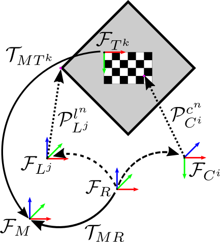
Figure 1: Calibration problem with all coordinate frames

III-B Mathematical Framework

For simplicity, assume there is only one target, one lidar and one camera as shown in Fig. 1. We will later extend it to multiple targets and sensors. Let us first consider the case of extrinsic lidar calibration to the robot frame as a separate problem. The problem can be written as follows: given a set of measured lidar keypoints, $\mathbf{P}^{l}_{L}=\{P^{l^{1}}_{L},\dots,P^{l^{N}}_{L}\}$, an initial calibration estimate, $T_{RL}$, as well as the set of corresponding ground truth keypoint locations expressed in the robot frame, $\mathbf{P}^{l}_{R}=\{P^{l^{1}}_{R},\dots,P^{l^{N}}_{R}\}$, estimate the robot to lidar frame transformation parameters. In this case, $N$ is the total number of lidar keypoints which depends on the number of target observations and the number of keypoints per target observation. To determine the ground truth location of the keypoints in the robot frame, we can use the location of the keypoints in the target frame (i.e., $P_{T}^{l^{i}}$) which are known a priori (e.g, hand measured or known due to target dimensions) and the high precision MCS measurements according to Eq. 1. For details on how measured lidar keypoints are extracted and how their corresponding ground truth values are determined, see Section III-D.

$$P^{l^{n}}_{R}=T_{RM}\>T_{MT}\>P^{l^{n}}_{T}$$ (1)

Using Eq. 1 and the initial calibration estimate, an error associated with the measurement of each lidar keypoint can be defined as a function of the calibration, as shown in Eq. 2. This error represents the Euclidean distance between the detected lidar point, expressed in the lidar frame, and its corresponding ground truth lidar point transformed to the lidar frame using the current calibration estimate. As the current calibration estimate converges to the true value, this error should diminish.

$$e_{l,n}(T_{RL})=P^{l^{n}}_{L}-T_{RL}^{-1}\>T_{RM}\>T_{MT}\>P^{l^{n}}_{T}$$ (2)

It is important to highlight a subtle difference between this formulation and many extrinsic calibration methodologies. Since we want this formulation to be applicable to any target design, we cannot assume that one sensor observation of a target is sufficient to fully constrain the pose of that target relative to the sensor. Instead, we assume there may be some degeneracies or symmetries in the target measurement. We instead rely on measured keypoints from all target observations to fully constrain the optimization. In other words, many calibration methods will extract a full 6 degree of freedom (DOF) estimate of the target pose from each observation, and one observation is expected to constrain the optimization, while multiple measurements increases accuracy. Instead, we store measured and expected keypoint locations for all observations, and all measurements are added to a single optimization problem as 3 DOF constraints, while relying on the diversity of the measurements to fully constrain the problem. We validate this assumption in Section IV with a degenerate calibration target.

Let us now consider the case of camera extrinsic calibration. Given a set of measured camera keypoints, $\mathbf{\rho}^{c}=\{\rho^{c^{1}},\dots,\rho^{c^{N}}\}$, an initial calibration estimate, $T_{RC}$, as well as the set of ground truth keypoint locations expressed in the robot frame, $\mathbf{P}^{c}_{R}=\{P^{c^{1}}_{R},\dots,P^{c^{N}}_{R}\}$, estimate the true calibration. Similar to the lidar case, an error term can be defined using the MCS measurements and the initial calibration. In this case, the camera-specific projection function $\pi(\dotsc)$ can be used to project the estimate of the ground truth keypoint location into the image plane. Eq. 3 shows this error function which represents the difference between the detected pixels and the projection of their corresponding keypoints after they have passed through the MCS transforms and the current calibration estimate. Note that in this work, we assume the intrinsics have already been calibrated, however, expanding this implementation to optimize over intrinsics is a straightforward extension that will be left for future work.

$$e_{c,n}(T_{RC})=\rho^{c^{n}}-\pi(T_{RC}^{-1}\>T_{RM}\>T_{MT}\>P^{c^{n}}_{T})$$ (3)

Now let us extend this formulation to any number of targets, lidars and cameras. Using the above two error terms, a single cost function can be defined as shown in Eq. 4.

$$\Psi(T_{RL},T_{RC})=\sum_{j=1}^{J}\sum_{k=1}^{K_{Li}}\sum_{n=1}^{N_{k,j}}e_{l,n}(T_{RL^{j}})+\sum_{i=1}^{I}\sum_{k=1}^{K_{Ci}}\sum_{n=1}^{N_{k,i}}e_{c,n}(T_{RC^{i}})$$ (4)

In Eq. 4, $J$ is the number of lidars, $I$ is the number of cameras, $K_{Lj}$ is the number of target observations for lidar $j$, $K_{Ci}$ is the number of target observations for camera $i$, $N_{k,j}$ is the number of keypoints for target observation $K_{Lj}$, and $N_{k,i}$ is the number of keypoints for target observation $K_{Ci}$. To solve this, a non-linear optimizer is used to find the set of $T_{RL}$ and $T_{RC}$ calibrations that minimise the cost function, $\Psi$. Note that in the current formulation, the calibration of each sensor can be solved independently since the measurements from each sensor are independent, and the calibrations are estimated relative to the same base frame, $F_{R}$. However, the optimization problem in this implementation was formulated as a single unified problem so that additional constraints can be added for joint measurements between sensors, as in the case of overlapping FOV sensors. Since we focus on calibration accuracy with no sensor FOV overlap, the trivial extension of the above objective function to incorporate joint target observations between any camera-lidar pair is omitted.

III-C Measurement Extractors

The intent of the measurement extractors is to reliably and automatically extract the target keypoints from lidar scans and camera images. Each type of target will have its own method for extracting the keypoints from the sensor data, however, some common data pre-processing can be applied to all data given the MCS measurements.

This work uses two types of targets with specific methods for extracting measured keypoints from the camera and lidar data. These targets serve as examples for how targets with and without distinct features visible to the camera and lidar can be used in the proposed formulation. The first target is a planar diamond shape with a checkerboard in the center and the second target is a plastic green cylinder (see Fig. 2). The diamond target was selected because the corners of the diamond can be easily detected as distinct features in the lidar scan as long as the lidar scan crosses all four edges of the target at least once. Similarly, the checkerboard on the diamond shape can be detected in images using OpenCV[23] for distinct camera keypoint measurements. The cylinder target shape was selected because it is easy to construct, motion tracking markers can be precisely installed along the axis of the cylinder, and a sparse 3D lidar can easily detect the cylindrical shape and orientation given a few beams have intersected the target. The cylinder target was also painted green to ensure easy detection in the images. This cylindrical target shows that targets can be used even when there is insufficient information to fully constrain the target pose with a single observation. As long as there is a sufficiently diverse dataset of observations, multiple measurements of an otherwise degenerate target measurement nonetheless constrain all calibration DOFs.

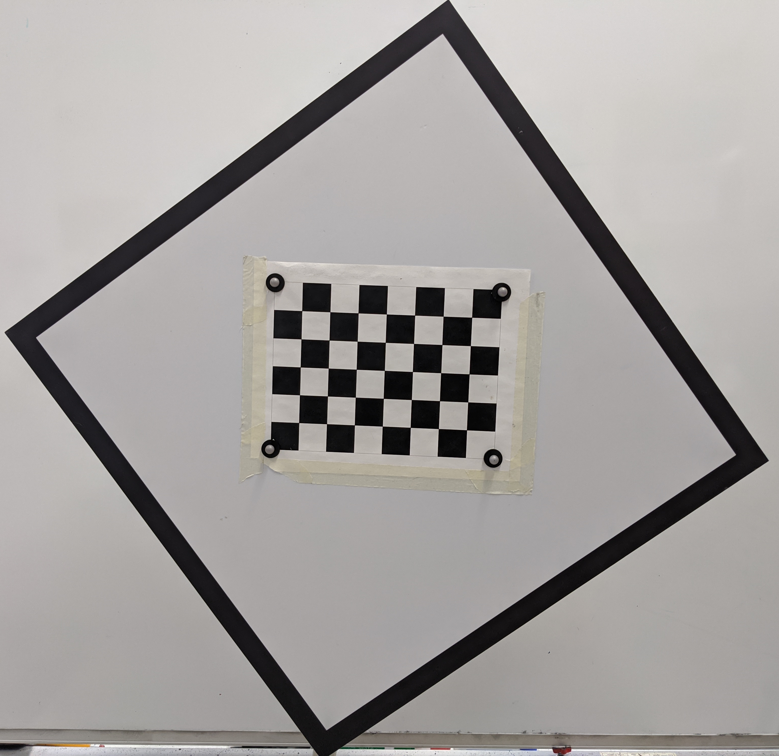
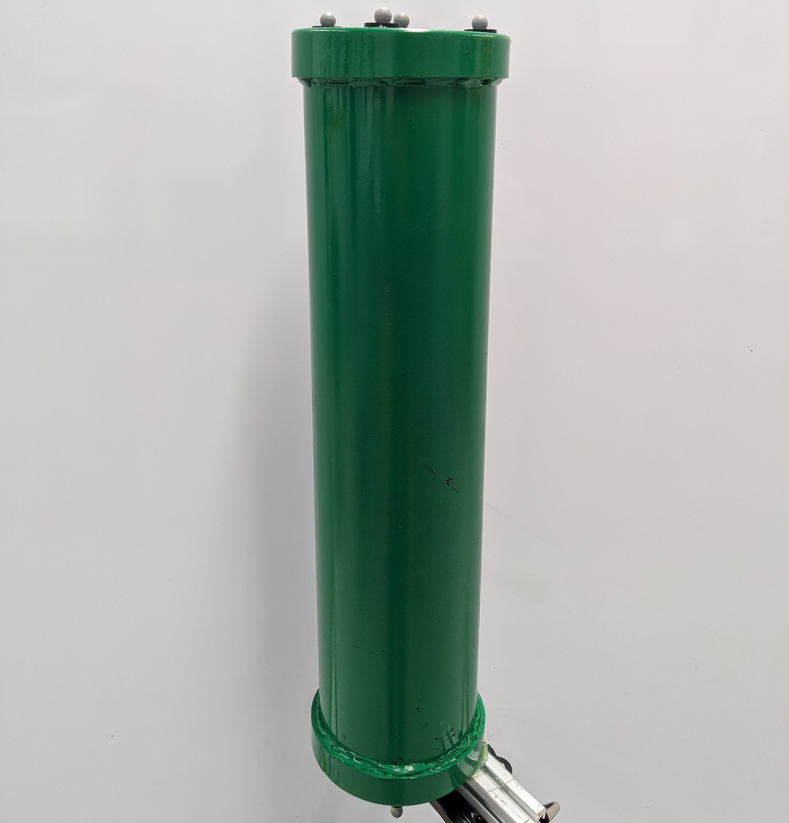
Figure 2: Custom targets including a diamond target with checkerboard (left) and a cylinder target (right)

There are common steps that can be taken to reduce the sensor data to a set of sub-sampled data that is known to contain the target. These steps are only possible due to the unique circumstances offered by the MCS, that is, that the pose of the target is always approximately known. We can take advantage of this information to ensure high quality measurements and reduce outliers, without user input. First, we step through our dataset and at each time step we calculate if the target is expected to be within the FOV of each sensor. Next, we check the velocity of the target relative to the robot and reject measurements with high motion which may induce motion distortion or may amplify the effect of any time synchronization errors. Once we know a target is likely to be observed by a sensor and is sufficiently stationary, we crop down the FOV of the sensor to only capture an area surrounding the estimated target location. This can be fine tuned based on our confidence in the initial calibration. After cropping the lidar data to the expected location of the target, we further narrow down the points that we expect to be part of the target by performing Euclidean clustering and selecting the most likely cluster. The cluster tolerance can be predetermined for each measurement given the known minimal angular resolution of the lidar and the known distance to the target. The most likely cluster is selected based on a weighted score using the difference between the target pose and the measured cluster error, and the difference between the measured volume and the known target volume. This results in a small subset of the collected data for both sensor types in which to identify the target, which increases our likelihood for properly detecting the correct keypoints on the target.

Let us consider the problem of detecting the keypoints on the diamond target once a subset data has been selected. As previously mentioned, the target keypoints to be detected are the 4 corner points of the diamond. To detect these points, a template cloud constructed to have the same dimensions as the real target is used and iterative closest point (ICP) is applied to align the template cloud to the reduced scan. The resulting transformation is then applied along with the MCS measurements to transform the known keypoints locations in the target frame ($P^{l^{n}}_{T}$) to the lidar frame ($F_{L^{j}}$) which then become the keypoint measurements. Since The diamond target camera keypoints are simply the checkerboard keypoints, these can be accurately detected by running the OpenCV checkerboard detector [23].

Contrary to the diamond target, the cylinder target does not have distinct keypoints that can be measured. The cylinder target extractor is therefore designed to use all the points along the edge of the shape as keypoints. Since these keypoints are not measurable by hand, correspondences cannot be guaranteed and therefore an iterative approach is necessary (for both correspondence search and optimization). To extract cylinder keypoints from the reduced lidar scan, ICP is performed with the template cloud, and points having correspondence distances below a certain threshold are kept. To extract the cylinder from the images, a color thresholding is first applied to keep only green pixels, then shape contours are detected using [24], and the contour points with the largest enclosed area are selected as the measured keypoints.

III-D Correspondence Estimation and Optimization

To construct the error terms presented in Eqns. 3 and 2, we must associate keypoint measurements in the sensor frame ($P_{L}^{l^{n}},\rho^{c^{n}}$), to the ground truth keypoint locations. Since each keypoint is not always uniquely identifiable, we estimate the correspondences between the measured points and the ground truth keypoints iteratively.

To solve this correspondence problem for a given target, we can take advantage of the MCS measurements and the current estimate of the calibration to perform a nearest neighbor search (NNS). First, the ground truth target keypoints are transformed from their target frames into the sensor frames. Following this step, the centroids of both point clouds are calculated, and the transformed keypoints are translated such that the centroids of both clouds align. A NNS is then performed to determine the correspondences between the measured keypoints and the original keypoints on the target. For the case of the camera measurements, the keypoints are also projected into the image plane and NNS is done on the 2D pixel coordinates.

Fig. 3 shows an example of the correspondence estimation for all four cases presented in this work. For the case of the cylinder target, since distinct keypoints are not measured, a template cloud with the same dimensions of the target is used and all points from the template cloud are converted to the sensor frame and used for correspondence search.

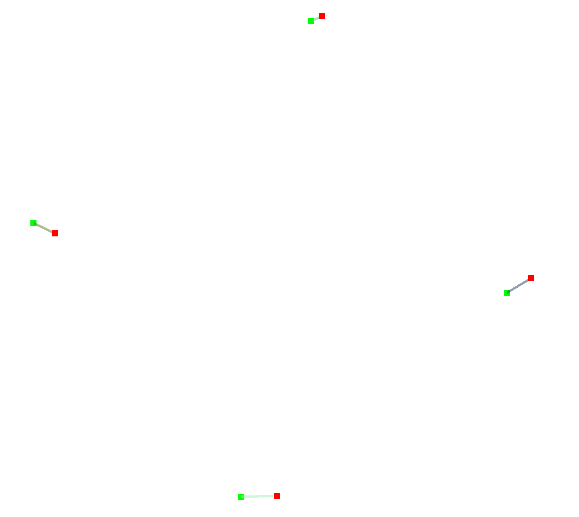
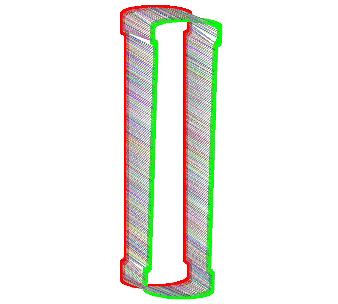
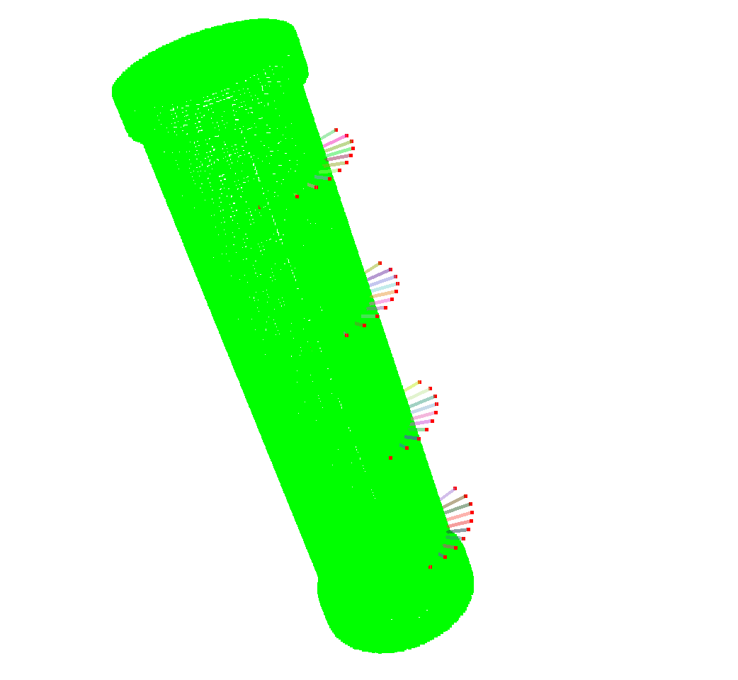
Figure 3: Example correspondence estimation: camera keypoints for diamond target (top left), lidar keypoints for diamond target (top right), camera keypoints for cylinder target (bottom left), lidar keypoints for cylinder target (bottom right). Red: measured keypoints. Green: transformed ground truth keypoints

The optimization of Eqn. 4 is solved using Levenberg-Marquadt (LM) optimization and implemented with Ceres. Since the original correspondences are often incorrect due to error in the initial calibrations used to transform the keypoints, the correspondence search and optimization are iterated until convergence. That is, once the optimizer converges, the correspondences are recalculated and a new optimization problem is constructed and solved. This process is iterated until either the change in total cost or the change in calibrations is below a threshold.

IV RESULTS

This section will discuss the validation procedure for the proposed calibration approach and present key results. The results will be presented for simulation and experimental data where simulation is used to test against known calibrations that have been perturbed. Both simulation and experimental data are validated using average keypoint reprojection error for the case of the camera calibrations, and average keypoint Euclidean distance error for the lidar calibrations.

IV-A Simulation Data

A simulation environment was created using Gazebo and the Robot Operating System (ROS) to simulate a MCS calibration environment with one camera and one Velodyne VLP-16 lidar. To simulate the camera, a simple pinhole camera with no lens distortion is used to avoid any possible issues with improper intrinsic calibrations. Gaussian noise was added to the pixel intensities measured by the simulated camera with a mean of 0 and standard deviation of 1.8. The lidar was simulated using Velodyne’s ROS simulator, with no noise added to the range or bearing measurements. To simulate the MCS, a ROS node was created that converts the model states provided by Gazebo to transform messages that describe the target motion relative to the map frame, and the robot frame motion relative to the map frame. These odometry messages have been designed to emulate the data format from a Vicon MCS. No measurement noise is added to the MCS measurements due to the high accuracy that these devices can achieve relative to the accuracy of the sensors being calibrated. The Vicon MCS can achieve a mean absolute error of 0.15 mm [21], which is orders of magnitude smaller than, for example, typical lidar error which are on the order of several centimeters.

Calibration results were obtained by selecting $N$ measurements of one particular target and documenting the mean and standard deviation of the errors. Target measurements are selected at different positions and orientations relative to the sensors to excite all extrinsic DOFs. For simulation data, the true calibrations are known, therefore the rotational and translational errors of the calibrations (i.e., transformations from sensor to robot frame) are presented. For the rotational error, the angles are converted to angle-axis representations and the absolute difference in the angle is presented. For the translational error, the absolute difference in the translation norms is presented. For the case of the camera calibration, the reprojection error is also presented by taking the norm of the vector between the projected points and the detected pixels. For the case of the lidar, the mean Euclidean error is presented which is calculated by taking the norm of the vector between the target keypoints transformed into the lidar frame and the detected keypoints in the lidar scan data. To validate the sensitivity of the proposed approach towards various initial calibration estimates, the known calibrations are perturbed by sampling linear and rotational perturbations from a random uniform distribution. For translational DOFs, perturbations are taken from -3 cm to +3 cm, and for rotational DOFs, perturbations are taken from -5 degrees to +5 degrees. The maximum perturbations are justified based on the maximum error that could be expected by hand measuring transformation between sensor centers.

Tables I and II show the lidar calibration results using the diamond target and the cylinder target, respectively. In both cases, tests were done with 5, 15, and 30 measurements of the target at different positions and orientations. In general, the mean and standard deviations of the sensor extrinsics and Euclidean errors are reduced as the number of measurements increases. Since no noise is added to the lidar measurements or MCS measurements, the proposed methodology converges to the solution with low errors using very few measurements. Looking at the diamond target results, a mean of 0.3 mm of translational error and 0.004 degrees of rotational error in the extrinsics is achieved after only 5 measurements. For the case of the cylinder target, the errors are higher and it does require larger number of measurements to converge. However, it can be argued that the cylinder target may be easier to construct in a way that the MCS markers can be precisely placed along the axis of the cylinder, whereas the diamond target could introduce errors if the MCS marker locations are not as precisely measured.

TABLE I: Simulated lidar calibration errors using the diamond target

Test	No.	Trans. (mm)		Rot. (deg)		Euc. (mm)
	Meas.	$\mu$	$\sigma$	$\mu$	$\sigma$	$\mu$	$\sigma$
1	30	0.1	1.7e-6	1.8e-3	5.1e-8	0.5	0.1
2	15	0.1	2.0e-6	2.4e-3	3.6e-7	0.4	0.6
3	5	0.3	4.3e-6	3.8e-3	3.5e-8	2.2	9.0

TABLE II: Simulated lidar calibration errors using the cylinder target

Test	No.	Trans. (mm)		Rot. (deg)		Euc. (mm)
	Meas.	$\mu$	$\sigma$	$\mu$	$\sigma$	$\mu$	$\sigma$
1	30	4.6	2.4	4.7e-2	3.4e-2	4.5	0.3
2	15	7.4	4.6	0.1	6.8e-2	5.0	0.3
3	5	88.0	64.2	1.6	2.0	7.8	0.7

Table III presents the results of camera calibration using the diamond target. Based on the performance of the diamond target in simulation, the results for the camera calibration using cylinder targets are not presented and are left to future work. Similar to the lidar calibration results, the camera calibration converges with only a few measurements. After 5 measurements, the mean translation error and rotational error are 0.1 mm and 0.03 degrees, respectively. The reduction in the errors as the number of measurements increases is less apparent in this case. This is likely because the calibration errors are so low with only 5 measurements, and increasing the number of measurements introduces the possibility of increased error due to motion blur or other such error sources.

TABLE III: Simulated camera calibration errors using the diamond target

Test	No.	Trans. (mm)		Rot. (deg)		Proj. (pixels)
	Meas.	$\mu$	$\sigma$	$\mu$	$\sigma$	$\mu$	$\sigma$
1	30	0.111	1.3e-6	0.035	9.2e-8	0.158	1.4e-8
2	15	0.066	3.6e-6	0.035	3.6e-6	0.167	6.2e-8
3	5	0.136	1.9e-6	0.034	1.3e-8	0.131	3.9e-7

To illustrate the calibration results, we can conveniently use the pose of the target at each measurement from the MCS to overlay results. Given the template cloud for each target, we can transform the template cloud points and the measured keypoints into the map frame using the initial, optimized, and ground truth calibration to see the accuracy of our calibration. Figure 4 shows one measurement example for each lidar target, where the blue points are the template cloud points transformed into the map frame using the ground truth calibration (i.e., the ground truth target pose), the green points are the scan points transformed to the map frame using the optimized calibrations, and the red points are the scan points converted to the map frame using the initial calibration (i.e., the perturbed ground truth calibration). The green points line up very well with the blue template cloud which visually demonstrates the accuracy of our calibration.

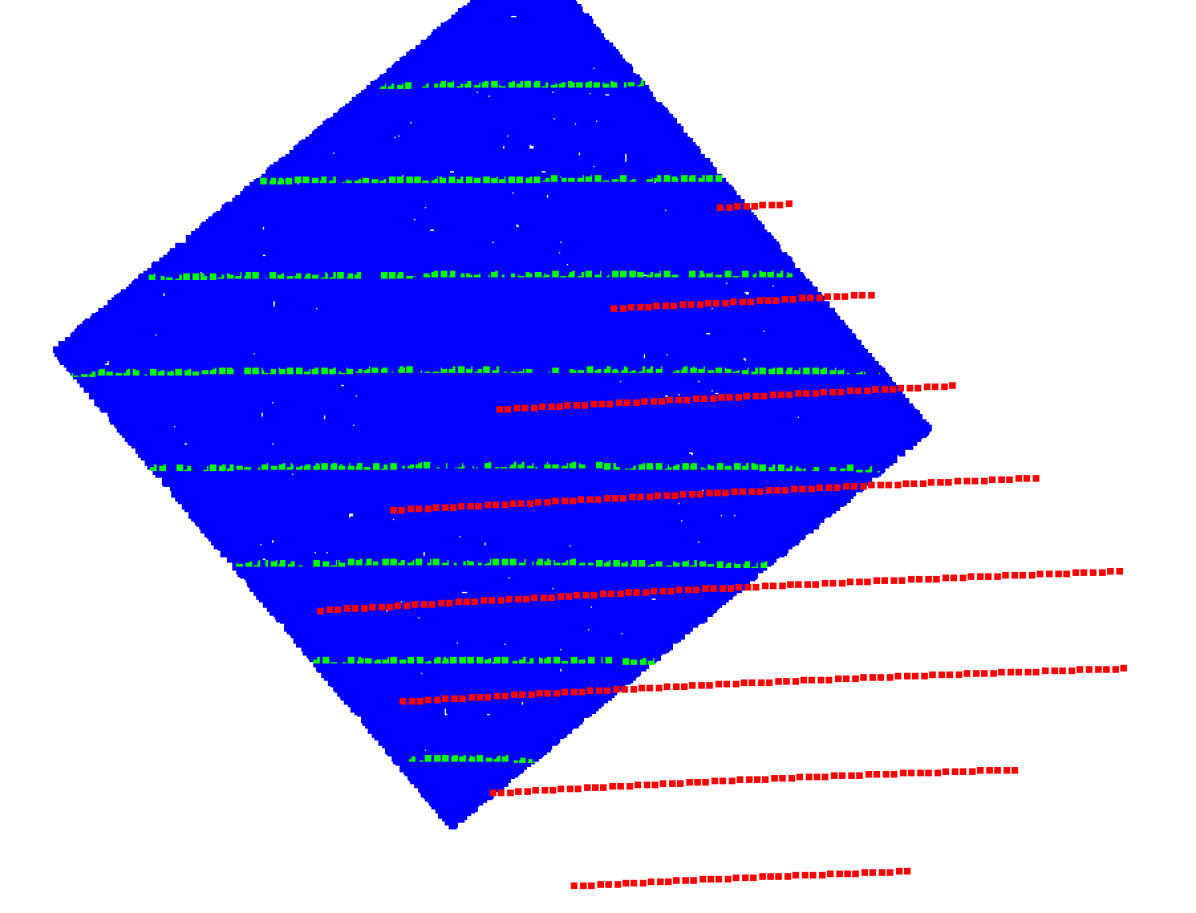
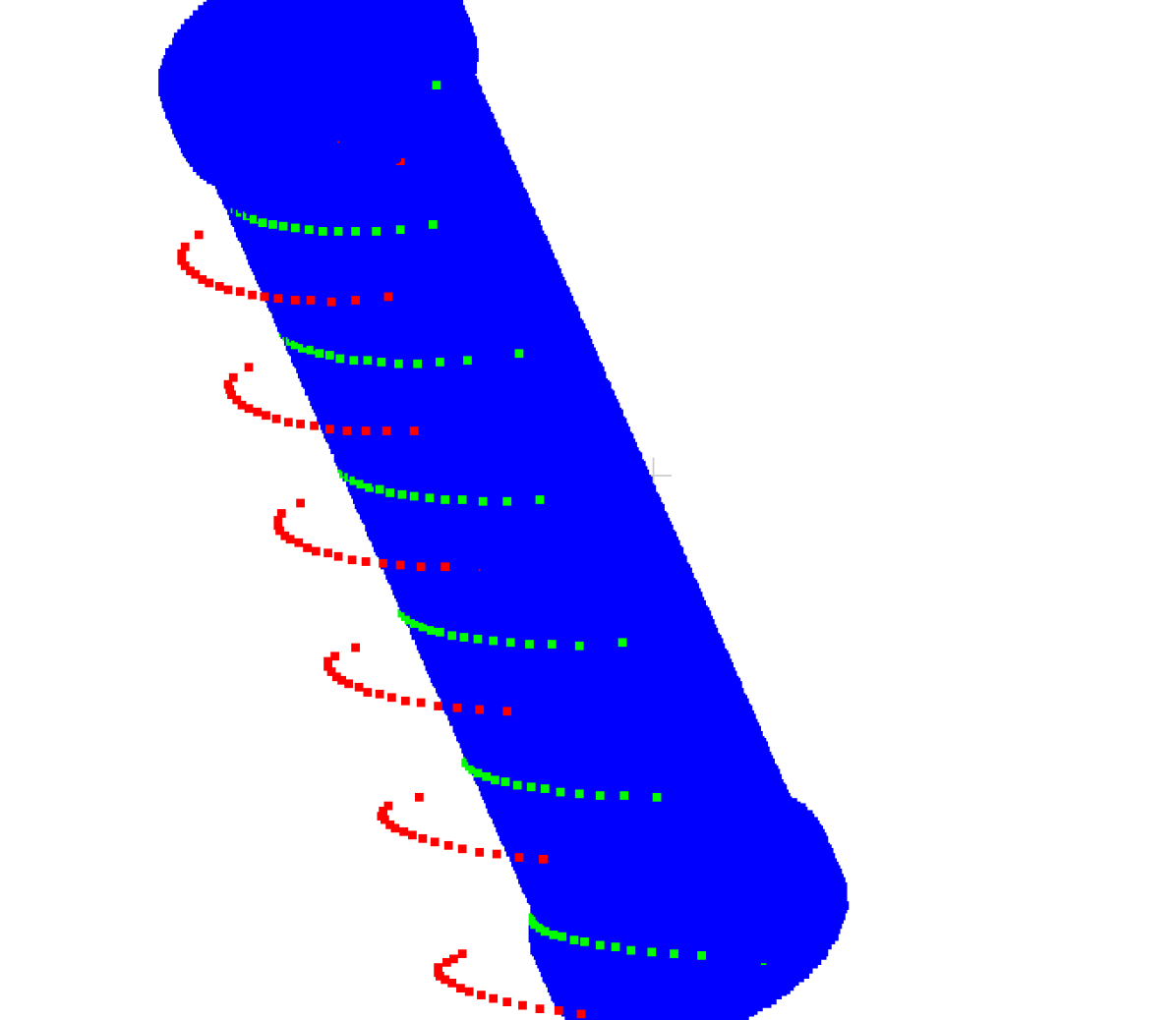
Figure 4: Example lidar calibration results using simulation data with diamond target (left) and cylinder target (right)

Figure 5 shows similar results for the camera calibration, however, the points are projected into the image plane and plotted on the image measurement for visualization. In this case, the keypoints and the outline of the diamond target are shown to better visualize the results.

Figure 5: Example camera calibration results using simulation data with diamond target (left) and cylinder target (right)

IV-B Experimental Data

The experimental setup is very similar to that of the simulation environment. A Clearpath Husky ground robot is equipped with a Velodyne VLP-16 lidar and a pre-calibrated (using a pinhole camera model with radtan lens distortion [22]) Flir BlackflyS camera. The MCS used in the experimental data is a Vicon MCS [21], and markers were setup on the targets (as shown in Fig 2) so that the MCS can directly measure the pose of the targets. All keypoint locations were hand measured a priori in these coordinate frames, and template clouds were generated with the coordinate centers aligning with that of the real targets. Furthermore, markers were added to the robot, ensuring good visibility by the MCS cameras. The location of the robot coordinate frame is irrelevant, since all calibrations are measured with respect to the same frame and therefore relative calibrations between all sensors can be determined.

Due to the sparsity of our experimental lidar data, tests showed that it was more effective to use all lidar points that come into contact with the diamond target, instead of using the corner estimates. Since the simulation results suggest that the calibrations should converge with at least 15 target measurements, this number of measurements was used for all experimental testing. For lidar calibration using the diamond target, an average Euclidean error of 12 mm was achieved, whereas the same error using the cylinder target was 16 mm. According to the manufacturer’s datasheet [25], the VLP-16 lidar shows a typical range error of +/-3 cm, suggesting that the +/- error of 1.2 cm to 1.5cm is well within the error limits that would be expected even with a perfect calibration. This demonstrates promising results for the lidar calibration given the high level of measurement noise in the sensor data.

Fig 6 shows an example of lidar calibration results on the experimental data. Once again, the blue points are the template clouds converted into the map frame given the MCS measurements. The green and red points are the scans points converted into the map frame using the optimized and initial calibrations, respectively. Despite the high noise in the lidar data, the green points visually align well with the blue template cloud.

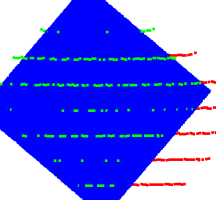
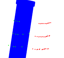
Figure 6: Example lidar measurement results with experimental data for the diamond (left) and cylinder (right)

Camera calibration using the diamond target was also validated with the experimental data. A higher than expected reprojection error was observed for the experimental dataset relative to the results from simulation. Using 5 measurements of the diamond target, an average reprojection error of 3.1 pixels was achieved, with additional measurements providing no further decrease in reprojection error. Possible sources of error in the experimental results include focus blur on all images, mismeasurement of target geometry, misalignment of the target frame location when creating the target, and timing errors between the MCS and camera image capture, since the camera was not hardware triggered. Nonetheless, these calibration results outperform state-of-the-art targetless methods. To compare results, we can convert our mean reprojection error to an approximate mean rotational error for each sensor calibration. Dividing the horizontal camera FOV by the image width, we get the rotational degree per pixel which can then be multiplied by the pixel error to get an approximate rotational error. Given a mean reprojection error of 3.1 pixels, our estimated rotational error is computed to be 0.07 degrees. This outperforms the targetless calibration methodology presented by Taylor et al. [17] who achieved rotational errors between 0.1 degrees and 0.4 degrees on each of the three principle axes.

V CONCLUSIONS

In this work, we show that a MCS can be used to perform extrinsic calibration of non-overlapping FOV lidar-camera systems without requiring a SLAM implementation. Our methodology results in a repeatable and accurate calibration common to traditional target-based approaches, without the overlapping FOV constraints. We validate this with experimental and simulation data, while also validating that our implementation can be extended to various target shapes or feature extraction methods. This new extrinsic calibration methodology removes any limitations on sensor configuration while ensuring we can maintain precise data fusion to support any downstream data processing application in robotics.

References

- [1] Q. Zhang and R. Pless, “Extrinsic calibration of a camera and laser range finder (improves camera calibration),” 2004 IEEE/RSJ International Conference on Intelligent Robots and Systems (IROS), vol. 3, pp. 2301–2306, 2004.
- [2] E. S. Kim and S. Y. Park, “Extrinsic calibration of a camera-LIDAR multi sensor system using a planar chessboard,” International Conference on Ubiquitous and Future Networks, ICUFN, vol. 2019-July, pp. 89–91, 2019.
- [3] A. Geiger, F. Moosmann, Ö. Car, and B. Schuster, “Automatic camera and range sensor calibration using a single shot,” Proceedings - IEEE International Conference on Robotics and Automation, pp. 3936–3943, 2012.
- [4] H. Alismail, L. D. Baker, and B. Browning, “Automatic calibration of a range sensor and camera system,” Proceedings - 2nd Joint 3DIM/3DPVT Conference: 3D Imaging, Modeling, Processing, Visualization and Transmission, 3DIMPVT 2012, pp. 286–292, 2012.
- [5] S. A. Rodriguez F., V. Frémont, and P. Bonnifait, “Extrinsic calibration between a multi-layer lidar and a camera,” IEEE International Conference on Multisensor Fusion and Integration for Intelligent Systems, pp. 214–219, 2008.
- [6] A. Velas, M., Spanel, M., Materna, Z., Herout, “Calibration of RGB Camera With Velodyne LiDAR,” in Conference on Computer Graphics, Visualization and Computer Vision, 2014.
- [7] C. Guindel, J. Beltran, D. Martin, and F. Garcia, “Automatic extrinsic calibration for lidar-stereo vehicle sensor setups,” IEEE Conference on Intelligent Transportation Systems, Proceedings, ITSC, vol. 2018-March, pp. 1–6, 2018.
- [8] J. Domhof, K. F. Julian, and K. M. Dariu, “An extrinsic calibration tool for radar, camera and lidar,” Proceedings - IEEE International Conference on Robotics and Automation, vol. 2019-May, pp. 8107–8113, 2019.
- [9] J. Kummerle, T. Kuhner, and M. Lauer, “Automatic Calibration of Multiple Cameras and Depth Sensors with a Spherical Target,” IEEE International Conference on Intelligent Robots and Systems, pp. 5584–5591, 2018.
- [10] J. Rebello, A. Fung, and S. L. Waslander, “Ac/dcc : Accurate calibration of dynamic camera clusters for visual slam,” in 2020 IEEE International Conference on Robotics and Automation (ICRA), pp. 6035–6041, 2020.
- [11] J. Castorena, U. S. Kamilov, and P. T. Boufounos, “Autocalibration of lidar and optical cameras via edge alignment,” ICASSP, IEEE International Conference on Acoustics, Speech and Signal Processing - Proceedings, vol. 2016-May, pp. 2862–2866, 2016.
- [12] J. Levinson and S. Thrun, “Automatic online calibration of cameras and lasers,” in Robotics: Science and Systems, 2013.
- [13] G. Pandey, J. R. McBride, S. Savarese, and R. M. Eustice, “Automatic targetless extrinsic calibration of a 3D lidar and camera by maximizing mutual information,” Proceedings of the National Conference on Artificial Intelligence, vol. 3, pp. 2053–2059, 2012.
- [14] Z. Taylor and J. Nieto, “Automatic calibration of lidar and camera images using normalized mutual information,” IEEE Conference on Robotics and Automation (ICRA), 2013.
- [15] T. Scott, A. A. Morye, P. Piniés, L. M. Paz, I. Posner, and P. Newman, “Exploiting known unknowns: Scene induced cross-calibration of lidar-stereo systems,” in 2015 IEEE/RSJ International Conference on Intelligent Robots and Systems (IROS), pp. 3647–3653, 2015.
- [16] A. Napier, P. Corke, and P. Newman, “Cross-calibration of push-broom 2D LIDARs and cameras in natural scenes,” Proceedings - IEEE International Conference on Robotics and Automation, pp. 3679–3684, 2013.
- [17] Z. Taylor and J. Nieto, “Motion-Based Calibration of Multimodal Sensor Extrinsics and Timing Offset Estimation,” IEEE Transactions on Robotics, vol. 32, no. 5, pp. 1215–1229, 2016.
- [18] N. Andreff, R. Horaud, and B. Espiau, “Robot Hand-Eye Calibration Using Structure-from-Motion,” The International Journal of Robotics Research, vol. 20, no. 3, pp. 228–248, 2001.
- [19] J. Heller, M. Havlena, A. Sugimoto, and T. Pajdla, “Structure-from-motion based hand-eye calibration using L infinity minimization,” Proceedings of the IEEE Computer Society Conference on Computer Vision and Pattern Recognition, pp. 3497–3503, 2011.
- [20] J. Jeong, Y. Cho, and A. Kim, “The Road is Enough! Extrinsic Calibration of Non-overlapping Stereo Camera and LiDAR using Road Information,” IEEE Robotics and Automation Letters, vol. 4, no. 3, pp. 2831–2838, 2019.
- [21] P. Merriaux, Y. Dupuis, R. Boutteau, P. Vasseur, and X. Savatier, “A study of vicon system positioning performance,” Sensors (Switzerland), vol. 17, no. 7, pp. 1–18, 2017.
- [22] V. Usenko, N. Demmel, and D. Cremers, “The double sphere camera model,” Proceedings - 2018 International Conference on 3D Vision, 3DV 2018, pp. 552–560, 2018.
- [23] G. Bradski, “The OpenCV Library,” Dr. Dobb’s Journal of Software Tools, 2000.
- [24] S. Suzuki and K. A. Be, “Topological structural analysis of digitized binary images by border following,” Computer Vision, Graphics and Image Processing, vol. 30, no. 1, pp. 32–46, 1985.
- [25] Velodyne LiDAR, Inc., 345 Digital Drive, Morgan Hill, CA 95037, Velodyne LiDAR PickTM real-time 3D LiDAR sensor, 2017.