Trainable Projected Gradient Method for Robust Fine-tuning

Abstract

Recent studies on transfer learning have shown that selectively fine-tuning a subset of layers or customizing different learning rates for each layer can greatly improve robustness to out-of-distribution (OOD) data and retain generalization capability in the pre-trained models. However, most of these methods employ manually crafted heuristics or expensive hyper-parameter searches, which prevent them from scaling up to large datasets and neural networks. To solve this problem, we propose Trainable Projected Gradient Method (TPGM) to automatically learn the constraint imposed for each layer for a fine-grained fine-tuning regularization. This is motivated by formulating fine-tuning as a bi-level constrained optimization problem. Specifically, TPGM maintains a set of projection radii, i.e., distance constraints between the fine-tuned model and the pre-trained model, for each layer, and enforces them through weight projections. To learn the constraints, we propose a bi-level optimization to automatically learn the best set of projection radii in an end-to-end manner. Theoretically, we show that the bi-level optimization formulation could explain the regularization capability of TPGM. Empirically, with little hyper-parameter search cost, TPGM outperforms existing fine-tuning methods in OOD performance while matching the best in-distribution (ID) performance. For example, when fine-tuned on DomainNet-Real and ImageNet, compared to vanilla fine-tuning, TPGM shows $22\%$ and $10\%$ relative OOD improvement respectively on their sketch counterparts. Code is available at https://github.com/PotatoTian/TPGM.

1 Introduction

Improving out-of-distribution (OOD) robustness such that a vision model can be trusted reliably across a variety of conditions beyond the in-distribution (ID) training data has been a central research topic in deep learning. For example, domain adaptation [46, 39], domain generalization [50, 25], and out-of-distribution calibration [33] are examples of related fields. More recently, large pre-trained models, such as CLIP [28] (pre-trained on 400M image-text pairs), have demonstrated large gains in OOD robustness, thanks to the ever-increasing amount of pre-training data as well as effective architectures and optimization methods. However, fine-tuning such models to other tasks generally results in worse OOD generalization as the model over-fits to the new data and forgets the pre-trained features [28]. A natural goal is to preserve the generalization capability acquired by the pre-trained model when fine-tuning it to a downstream task.

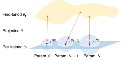
Figure 1: Illustration of TPGM. TPGM learns different weight projection radii, $\gamma$, for each layer between a fine-tuned model $\theta_{t}$ and a pre-trained model $\theta_{0}$ and enforces the constraints through projection to obtain a projected model $\tilde{\theta}$.

A recent empirical study shows that aggressive fine-tuning strategies such as using a large learning rate can decrease OOD robustness [41]. We hypothesize that the forgetting of the generalization capability of the pre-trained model in the course of fine-tuning is due to unconstrained optimization on the new training data [44]. This conjecture is not surprising, because several prior works, even though they did not focus on OOD robustness, have discovered that encouraging a close distance to the pre-trained model weights can improve ID generalization, i.e., avoiding over-fitting to the training data [44, 9]. Similarly, if suitable distance constraints are enforced, we expect the model to behave more like the pre-trained model and thus retain more of its generalization capability. The question is where to enforce distance constraints and how to optimize them?

Several works have demonstrated the importance of treating each layer differently during fine-tuning. For example, a new work [22] discovers that selectively fine-tuning a subset of layers can lead to improved robustness to distribution shift. Another work [31] shows that optimizing a different learning rate for each layer is beneficial for few-shot learning. Therefore, we propose to enforce a different constraint for each layer. However, existing works either use manually crafted heuristics or expensive hyper-parameter search, which prevent them from scaling up to large datasets and neural networks. For example, the prior work [31] using evolutionary search for hyper-parameters can only scale up to a custom 6-layer ConvNet and a ResNet-12 for few-shot learning. The computation and time for searching hyper-parameters become increasingly infeasible for larger datasets, let alone scaling up the combinatorial search space to all layers. For example, a ViT-base [37] model has 154 trainable parameter groups including both weights, biases, and embeddings. This leads to a search space with more than $10^{45}$ combinations even if we allow only two choices per constraint parameter, which makes the search prohibitively expensive.

To solve this problem, we propose a trainable projected gradient method (TPGM) to support layer-wise regularization optimization. Specifically, TPGM adopts trainable weight projection constraints $\gamma$, which we refer to as projection radii, and incorporates them in the forward pass of the main model to optimize. Intuitively, as shown in Fig. 1, TPGM maintains a set of weight projection radii $\gamma$ i.e., the distance between the pre-trained model ($\theta_{0}$) and the current fine-tuned model ($\theta_{t}$), for each layer of a neural network and updates them. The projection radii control how much ”freedom” each layer has to grow. For example, if the model weights increase outside of the norm ball defined by $\gamma$ and $\|\cdot\|$, the projection operator will project them back to be within the constraints. To learn the weight projection radii in a principled manner, we propose to use alternating optimization between the model weights and the projection radii, motivated by formulating fine-tuning as a bi-level constrained problem (Sec. 3.1). We theoretically show that the bi-level formulation could explain the behavior of TPGM (Sec. 3.4).

Empirically, we conduct thorough experiments on large-scale datasets, DomainNet [27] and ImageNet [4], using different architectures. Under the premise of preserving ID performance, i.e., OOD robustness should not come at the expense of worse ID accuracy, TPGM outperforms existing approaches with little effort for hyper-parameter tuning. Further analysis of the learned projection radii reveals that lower layers (layers closer to the input) in a network require stronger regularization while higher layers (layers closer to the output) need more flexibility. This observation is in line with the common belief that lower layers learn more general features while higher layers specialize to each dataset [26, 29, 45, 41]. Therefore, when conducting transfer learning such as fine-tuning, we need to treat each layer differently. Our contributions are summarized below.

• We propose a trainable projected gradient method (TPGM) for fine-tuning to automatically learn the distance constraints for each layer in a neural network during fine-tuning.

• We conduct experiments on different datasets and architectures to show significantly improved OOD generalization while matching ID performance.

• We theoretically study TPGM using linear models to show that bi-level optimization could explain the regularization capability of TPGM.

2 Related Works

Fine-tuning to Boost ID Performance. SpotTune [11] introduces an additional policy network, which outputs a linear interpolation ratio between the pre-trained model ($\theta_{0}$) and fine-tuned model ($\theta_{t}$) based on the input. Instead of directly regularizing the weight space, DELTA [23] proposes to regularize the output (feature maps) of $\theta_{0}$ and $\theta_{t}$. However, SpotTune introduces an additional network and needs to keep both the pre-trained model and fine-tuned model for inference. DELTA specifically regularizes feature maps generated by convolution layers. In this work, we focus more on general methods, which do not increase inference costs and are applicable to a broader range of models. L2-SP [44] proposes an explicit inductive bias for fine-tuning. Specifically, it uses an L2 regularization to minimize the distance between $\theta_{0}$ and $\theta_{t}$. Most recently, MARS-SP [8] adopts the projected gradient method (PGM) to constrain $\theta_{t}$ within a small sphere centered on the pre-trained model $\theta_{0}$. MARS-SP has shown great performance against its prior works. However, we find it very sensitive to hyperparameter tuning. Nonetheless, our work is inspired by and improves PGM by 1) incorporating trainable weight projection radii for each layer and 2) developing a bi-level optimization algorithm to learn them.

Fine-tuning to Improve OOD Generalization. As the size of the target dataset increases and better architectures are developed, the benefit from pre-training on the target ID performance diminishes [13]. However, the power of pre-training goes beyond boosting ID performance. A recent work [40] finds that using pre-trained models can greatly improve robustness on OOD datasets and uncertainty-related tasks such as confidence calibration [10] and OOD detection [5]. Moreover, the fine-tuning strategy used also plays an important role in improving OOD generalization. LP-FT [21] shows that simultaneously fine-tuning the last linear layer and the feature backbone can distort pre-trained features and thus decreases OOD generalization. A simple strategy of linear probing, i.e., training only the classifier layer, followed by fine-tuning the entire network can greatly mitigate this distortion and improve OOD generalization. WISE [41] demonstrates impressive OOD generalization gains by linearly interpolating $\theta_{0}$ and $\theta_{t}$. However, this strategy only applies to image-text pre-trained models with zero-shot classifiers such as CLIP [28] because WISE requires the model to have linear connectivity. In most cases, linear interpolation between two models results in no better performance than random initialization [7].

3 Method

In the introduction, we motivated the benefit of explicitly maintaining distance constraints between a pre-trained model and a fine-tuned model [44, 9]. However, it is not clear how to search the space of hyper-parameters (distance constraints) especially if we want to do this per layer as the search space grows combinatorially with the number of layers. To this end, we pose the search as a bi-level constrained optimization problem in Sec. 3.1 and introduce closed-form projection in Sec. 3.2. Then we present the proposed TPGM algorithm in Sec. 3.3. Finally, we theoretically show that the bi-level optimization design enables TPGM to learn different constraints for each layer in Sec. 3.4.

3.1 Fine-tuning as a Bi-level Constrained Problem

Machine learning algorithms usually tune hyper-parameters, e.g., learning rate, weight decay, etc., on a validation split. Mathematically, this procedure is equivalent to a bi-level minimization problem. Let $(x,y)$ denote a pair of input data and $\mathcal{L}(\cdot)$ denote the task loss function. The minimization problem can be written as

$$\min_{\lambda|(x,y)\in\mathcal{D}_{val}}\mathcal{L}(x,y;\operatorname*{arg\,min}_{\theta_{t}|(x,y)\in\mathcal{D}_{tr}}\mathcal{L}(x,y;\theta_{t},\lambda),\lambda),$$ (1)

where $\theta_{t}$ denotes the trainable model weights and $\lambda$ denotes the hyper-parameters such as learning rate. $\mathcal{D}_{tr}$ is the set of training data and $\mathcal{D}_{val}$ is the set of validation data.

Now, we extend this formulation to fine-tune a pre-trained model. Specifically, it has been shown that maintaining a close distance to the pre-trained model improves a model’s generalization and robustness [16, 44]. A recent paper [9] formalizes the concept of maintaining distance as a constrained optimization problem, in which the distance between the new model and the pre-trained model is measured by matrix norms $\|\cdot\|_{*}$. Mathematically, combined with Eq. 1, we further extend the constrained optimization to a bi-level constrained minimization problem as

$$\min_{\lambda,\gamma|(x,y)\in\mathcal{D}_{val}}\mathcal{L}(x,y;\operatorname*{arg\,min}_{\theta_{t}|(x,y)\in\mathcal{D}_{tr}}\mathcal{L}(x,y;\theta_{t},\lambda),\lambda),$$ (2)

$$\quad\text{s.t.}\quad\|\theta_{t}-\theta_{0}\|_{*}\leq\gamma,$$

where $\|\theta_{t}-\theta_{0}\|_{*}$ denotes a norm induced distance between the pre-trained model $\theta_{0}$ and the new model $\theta_{t}$. Optimizing Eq. 2 enforces the model to stay within a distance $\gamma$ from the pre-trained model.

3.2 Projected Gradient Method

One method to optimize a constrained problem is projected gradient method (PGM) [18]. PGM projects the updated model weights to be within the constraint, i.e., $\|\theta_{t}-\theta_{0}\|_{*}\leq\gamma$. However, in general, most projection operations are optimization problems themselves with only a few exceptions having closed from solutions. One example is L2-norm projection $\Pi_{l2}$. Projecting a matrix $\theta_{t}$ to $\gamma$ distance away, measured by L2 norm, from another matrix $\theta_{0}$ is a closed form operation as shown in Eq. 3.

$$\Pi_{l2}(\theta_{0},\theta_{t},\gamma):\tilde{\theta}=\theta_{0}+ \frac{1}{\text{max}\left(1,\frac{\|\theta_{t}-\theta_{0}\|_{2}}{\gamma}\right)}(\theta_{t}-\theta_{0})$$ (3)

The prior work [9] uses the maximum absolute row sum (MARS) matrix norm because it has a closed form approximation that enables fast projection without optimization as well. The MARS approximate projection operator $\Pi_{mars}$ is defined in Eq. 4.

$$\Pi_{mars}(\theta_{0},\theta_{t},\gamma):\tilde{\theta}=\theta_{0}+ \frac{1}{\text{max}\left(1,\frac{\|\theta_{t}-\theta_{0}\|_{\infty}}{\gamma}\right)}(\theta_{t}-\theta_{0})$$ (4)

$\|\cdot\|_{\infty}$ denotes the MARS matrix norm, $\|A\|_{\infty}=\max_{j}\sum_{i=1}|A_{j,i}|$. Even though we use closed-form projection to avoid additional computation, the projection radius $\gamma$ needs to be pre-determined. Searching for a single weight projection parameter for all layers is already challenging because the scale of $\gamma$ is unknown let alone tailoring a weight projection radius to each layer. In this paper, we do not investigate specific properties of projections, which are orthogonal to our contributions. Therefore, we will benchmark both projections and report the one with better results and leave the comparison to Appendix.

3.3 Trainable Projected Gradient Method (TPGM)

Inspired by the projected gradient method, we propose a trainable approach to solve the bi-level constrained problem in Eq. 2 by integrating the projection operator in Eq. 3 or Eq. 4 into the forward pass of a model, through which the weight projection radii $\gamma$ can be learned through backpropagation. Specifically, the algorithm consists of three functions: model update, projection update, and projection. A summary of TPGM is presented in Alg. 1 and details of the projection update function are in Alg. 2.

Data: $\mathcal{D}_{tr}$,$\mathcal{D}_{val}$

Result: $\tilde{\theta}_{t+1}$

Initialize $\tilde{\theta}_{0}=\theta_{0},\gamma_{0}=\epsilon$

for $t=\{0,...,T-1\}$ do

       $\theta_{t+1}=\theta_{t}-\eta_{t}\nabla_{\theta}\mathcal{L}(x,y;\tilde{\theta_{t}})\quad x,y\in\mathcal{D}_{tr}$

       if $t$ mod $f_{proj}$ $==0$ then

             $\gamma_{t+1}=\text{ProjectionUpdate}(\mathcal{D}_{val},\theta_{0},\theta_{t+1},\gamma_{t})$

             $\tilde{\theta}_{t+1}=\Pi(\theta_{0},\theta_{t+1},\gamma_{t+1})$

       end if

      

end for

Algorithm 1 TPGM

Data: $\mathcal{D}_{val}$

Result: $\gamma_{t+1}$

for $\tau=\{0,...,T_{proj}-1\}$ do

       $\tilde{\theta}=\Pi(\theta_{0},\theta_{t+1},\gamma_{\tau})$

       $\gamma_{\tau+1}=\gamma_{\tau}-\zeta\nabla_{\gamma}\mathcal{L}(x,y;\tilde{\theta})\quad x,y\in\mathcal{D}_{val}$

end for

Algorithm 2 ProjectionUpdate

Model Update. TPGM first takes an unconstrained gradient descent step. Let $\theta_{t+1}$ denote the updated model parameters at the gradient descent step $t$ for $t\geq 0$ where $\theta_{0}$ denotes the pre-trained initialization. This update is calculated on the loss function $\mathcal{L}(x,y;\theta_{t})$ where $(x,y)$ are sampled training data, i.e., $(x,y)\in\mathcal{D}_{tr}$. This corresponds to a regular gradient descent step in the conventional setting and the inner minimization in Eq. 2. For example, if vanilla SGD is used in this step, then,

$$\theta_{t+1}=\theta_{t}-\eta_{t}\nabla_{\theta}\mathcal{L}(x,y;\theta_{t}),\quad(x,y)\in\mathcal{D}_{tr}.$$

Any other optimizers, e.g., Adam [20], can be used instead.

Projection Update. The projection update function optimizes the weight projection parameters $\gamma_{t}$ iteratively. As shown in Alg. 2, the optimization loops for $T_{proj}$ steps. In Alg. 2, we use SGD as an example for clarity. Any other optimizer can be used. Specifically, using $\theta_{t+1}$ and the closed form projection operation in Eq. 3 (or Eq. 4), we construct a projected model $\tilde{\theta}$ with a trainable projection parameter $\gamma_{t}$ for $t\geq 0$ for each layer, where $\gamma_{0}$ is initialized to a small value $\epsilon$. Then, we optimize the projection parameters using the loss function $\mathcal{L}(x,y;\gamma_{t})$ where $(x,y)$ are sampled validation data, i.e., $(x,y)\in\mathcal{D}_{val}$. Crucially, in this step, only the weight projection parameters $\gamma_{t}$ are updated while the updated model $\theta_{t+1}$ remains frozen. In other words, no gradients of the model are calculated on the validation data. This is important to avoid contamination of the validation data. The projection update function corresponds to the outer minimization of the constrained problem in Eq. 2.

Projection. Finally, after a new set of projection parameters $\gamma_{t}$ is updated, we apply the learned projection radii to the updated model $\theta_{t+1}$ using Eq. 3 (or Eq. 4). This amounts to enforcing the constraint $\|\theta-\theta_{0}\|_{*}\leq\gamma$ in Eq 2. The projection update and projection functions can be called frequently controlled by a hyperparameter ($f_{proj}$ in Alg. 1). We will show that for certain pre-trained models, it is sufficient to only call these two functions once at the end of the training, i.e., when $f_{proj}=T-1$ (Sec. 4.2). Moreover, we found that in a few cases, TPGM could lead to under-fitting because of its iterative nature. However, the problem can be easily mitigated with total variation smoothing [1, 3]. Since we only observed this in one setting in our experiments, we defer the discussion to Appendix 5.3.

We summarize TPGM in Alg. 1. Intuitively, TPGM maintains a set of weight projection parameters for each layer of a neural network and updates them. The projection parameters control how much “freedom” each layer has to grow. As we will observe later, when fine-tuning a model, layers close to the input generally require smaller changes than layers close to the output. This property helps preserve generalization capabilities obtained by the pre-trained model. TPGM inevitably adds some computation overhead. We provide additional discussion on it in Appendix 5.9.

3.4 Bi-level Optimization

Following a common strategy in studying transfer learning [42, 36, 6, 43, 41], we theoretically study TPGM using linear models and explain why optimizing the bi-level problem in Eq. 2 could enable the regularization capability of TPGM.

Problem Setup. Let $x\in\mathbb{R}^{d}$ denote an ID data and the corresponding label $y$ is generated by a ground truth linear model $\theta_{*}\in\mathbb{R}^{d}$, i.e., $y=\theta_{*}^{T}x$. To construct the training set, we sample $n$ training data, where $n<d$, and stack the sampled data into a data matrix $\mathbf{X}_{tr}\in\mathbb{R}^{d\times n}$. Accordingly, the labels form a vector $\mathbf{Y}_{tr}=\mathbf{X}_{tr}^{T}\theta_{*}\in\mathbb{R}^{n}$. The training goal is to minimize the empirical loss.

$$\mathcal{L}(\mathbf{X}_{tr},\mathbf{Y}_{tr};\theta)=\|\mathbf{X}_{tr}^{T}\theta-\mathbf{Y}_{tr}\|_{2}$$ (5)

Note that this forms an over-parameterized linear system, i.e., there are more parameters than equations, because $n<d$. This is similar to how modern neural networks are over-parameterized with respect to the data.

Complementary Decomposition using SVD. For the analysis, we make an independence assumption on the data matrix $\mathbf{X}_{tr}$. This assumption exists for notation simplicity and can be relaxed easily.

Assumption 1.

Let the $n$ training data be linearly independent. The following SVD exists for the data matrix $\mathbf{X}_{tr}$.

$$\mathbf{X}_{tr}=\mathbf{U}\mathbf{\Sigma}\mathbf{V}^{T},\quad\mathbf{U}\in\mathbb{R}^{d\times n},\mathbf{\Sigma}\in\mathbb{R}^{n\times n},\mathbf{V}\in\mathbb{R}^{n\times n}.$$

Consequently, we can decompose any vector $x\in\mathbb{R}^{d}$ into two components, $x=\mathbf{U}\tau+\mathbf{U}_{\bot}\tau_{\bot}$, where $\mathbf{U}$ is the basis for the span of training samples, $\mathbf{U}_{\bot}\in\mathbb{R}^{d\times(d-n)}$ is the basis for the complementary subspace, and $\tau\in\mathbb{R}^{n}$, $\tau_{\bot}\in\mathbb{R}^{d-n}$ are the corresponding coordinates. There are infinitely many solutions to Eq. 5 because this is an over-parameterized system.

Definition 1.

We denote a projected model as $\tilde{\theta}=\theta_{0}+\alpha(\theta-\theta_{0})$ (obtained using Eq. 3 or Eq. 4), where $\theta$ is one minimizer of Eq. 5, $\theta_{0}$ is the pre-trained model and $0\leq\alpha\leq 1$ is the projection ratio.

To quantify the effects of projection $\alpha$, we can look at the average performance of the projected model $\tilde{\theta}$ on test data. Consequently, we investigate the expected loss of the projected model over the entire data space.

$$\mathbb{E}[\mathcal{L}(x,y;\tilde{\theta})]=\mathbb{E}\left[\left\|{\tilde{\theta}}^{T}x-y\right\|_{2}\right]$$ (6)

We provide the following theorem to shed light on how projection affects the expected loss and what it depends on.

Theorem 1.

Let Assumption 1 hold, the expected loss of $\tilde{\theta}$ in Eq. 6 is upper bounded as the following,

$$\mathbb{E}\left[\left\|\tilde{\theta}^{T}x-y\right\|_{2}\right] \leq\underbrace{(1-\alpha)\epsilon{\tau}}_{in-span}+\underbrace{\left(\epsilon+\alpha\left\|{\theta}-\theta_{0}\right\|_{2}\right){\tau}_{\bot}}_{out-span},$$ (7)

where $\epsilon=\left\|{\theta}_{0}-\theta_{*}\right\|_{2}$ and ${\tau}\doteq\mathbb{E}[\|\tau\|_{2}]$, ${\tau}_{\bot}\doteq\mathbb{E}[\|\tau_{\bot}\|_{2}]$. A complete proof is provided in Appendix 5.2.

The upper bound in Thm. 1 has two components, risk due to components in the training data span (in-span) and risk due to components in the complementary subspace (out-span). To minimize the expected loss, one will expect $\alpha$ to be dependent on the value of $\epsilon$. Recall that the quantity $\epsilon$ is the distance between the pre-trained model and the ground truth model and can be viewed as a measure of how “good” the pre-trained model is. Therefore, we expect two types of behaviors from $\alpha$ depending on $\epsilon$:

• When $\epsilon$ is small, $\alpha$ needs to be smaller to minimize the second component, meaning stronger projection.

• When $\epsilon$ is large, $\alpha$ needs to be larger to minimize the first component, meaning weaker projection.

The theorem indicates that if we optimize the projected model $\tilde{\theta}$ on a separate batch of data, different from the data the model gradients are calculated on, the projection ratio $\alpha$ will seek to balance between fitting the training data (in-span) and generalizing to new data (out-span). For example, when $\epsilon$ is small, i.e., the pre-trained model is close to the optimal model, the formulation encourages stronger projection.

Furthermore, as prior works have found that lower layers tend to learn more general features while higher layers specialize to a specific dataset, $\epsilon$ is likely to be smaller for the lower layers and larger for higher layers because pre-trained models likely have learned very good low-level general features [26, 29, 45, 41]. This offers one explanation of why TPGM automatically learns different constraints for each layer. Therefore, we hypothesize that optimizing the projection radii on a dataset sampled separately from the training data, e.g., the validation dataset, is essential to learning different constraints for each layer.

4 Experiments

Overview. To validate TPGM, we conduct experiments on large-scale datasets using different architectures. The experiments are split into two sections depending on the specific architecture used. In Sec. 4.1, we use ResNet [14] with a CLIP pre-trained ResNet50 [28] and an ImageNet pre-trained MOCO-V3 ResNet50[2] as the pre-trained models. In Sec. 4.2, we use Vision Transformers [37] with a CLIP pre-trained ViT-B model [28].

Datasets. For the ResNet experiments, we use DomainNet [27] (0.6M images over 345 classes) as the benchmark. DomainNet has five domains: real, sketch, painting, inforgraph, and clipart. We use the real domain as the ID fine-tuning domain (with held-out test data to test ID performance) and the rest as the OOD domains. For the Transformer experiments, we use ImageNet-1K[4] as the fine-tuning dataset. For the ID test dataset, we add ImageNet-V2 [30] in addition to ImageNet-1K. For the OOD test datasets, we use ImageNet-A [17], ImageNet-R [15], and ImageNet-S [38]. No OOD data are used during training.

4.1 Fine-Tuning a Pre-trained ResNet

Table 1: DomainNet Results using CLIP pre-trained ResNet50 with 100$\%$ Real Data. TPGM improves OOD performance significantly even when a zero-shot classifier is not available.

	ID	OOD				Statistics
	Real	Sketch	Painting	Infograph	Clipart	OOD Avg.	ID $\Delta$ ($\%$)	OOD $\Delta$ ($\%$)
Vanilla FT	80.93 (0.08)	31.81 (0.06)	41.02 (0.10)	20.29 (0.08)	43.59 (0.15)	34.18	0.00	0.00
LP	52.56 (0.09)	20.05 (0.21)	24.92 (2.49)	19.18 (0.46)	21.15 (0.18)	21.33	-35.05	-37.60
PF [19]	78.27 (0.11)	36.77 (0.32)	42.13 (0.35)	24.71 (0.18)	43.31 (0.53)	36.73	-3.29	7.46
L2-SP [44]	82.07 (0.09)	36.67 (0.11)	45.62 (0.35)	22.97 (0.42)	47.78 (0.30)	38.26	1.40	11.94
MARS-SP [9]	77.19 (0.63)	25.33 (1.07)	33.43 (2.06)	14.81 (0.43)	39.20 (0.74)	28.19	-4.62	-17.53
LP-FT [21]	80.82 (0.95)	34.85 (1.93)	44.03 (0.05)	22.23 (2.01)	46.13 (2.34)	36.81	-0.14	7.69
TPGM	83.64 (0.01)	38.78 (0.42)	43.11 (0.25)	28.70 (0.31)	48.01 (0.25)	39.65	3.34	16.01

Table 2: DomainNet Results using MOCO-V3 pre-trained ResNet50 Results with 100$\%$ Real Data. TPGM improves OOD generalization using a self-supervised pre-trained model while improving ID performance.

	ID	OOD				Statistics
	Real	Sketch	Painting	Infograph	Clipart	OOD Avg.	ID $\Delta$ ($\%$)	OOD $\Delta$ ($\%$)
Vanilla FT	81.99 (0.03)	31.52 (0.33)	42.89 (0.53)	18.51 (0.28)	44.98 (0.24)	34.47	0.00	0.00
LP	73.01 (0.03)	24.10 (0.23)	39.56 (0.15)	12.27 (0.02)	30.38 (0.08)	26.58	-10.96	-22.90
PF [19]	78.27 (0.03)	27.72 (0.07)	39.74 (0.12)	15.56 (0.08)	38.18 (0.12)	30.30	-4.55	-12.11
L2-SP [44]	81.51 (0.02)	34.91 (0.22)	45.76 (0.16)	18.97 (0.11)	45.29 (0.18)	36.23	-0.59	5.09
MARS-SP [9]	81.89 (0.01)	34.44 (2.54)	45.05 (1.91)	19.97 (1.48)	46.36 (1.29)	36.45	-0.13	5.74
LP-FT [21]	82.92 (0.01)	34.50 (0.22)	45.42 (0.31)	20.12 (0.43)	47.11 (0.27)	36.79	1.13	6.72
TPGM	82.66 (0.13)	35.35 (0.33)	46.20 (0.20)	20.13 (0.12)	45.75 (0.12)	36.86	0.82	6.91

Table 3: DomainNet Results using CLIP pre-trained ResNet50 with 10$\%$ Real Data. TPGM adjusts to the size of the fine-tuning dataset by imposing stronger per-layer constraints.

	ID	OOD				Statistics
	Real	Sketch	Painting	Infograph	Clipart	OOD Avg.	ID $\Delta$ ($\%$)	OOD $\Delta$ ($\%$)
Vanilla FT	57.35 (1.43)	17.48 (0.68)	25.60 (0.70)	10.30 (1.57)	23.01 (0.65)	19.10	0.00	0.00
LP	47.19 (0.93)	17.81 (0.25)	22.71 (2.08)	17.13 (0.75)	17.59 (0.69)	18.81	-17.71	-1.52
PF [19]	71.04 (0.91)	27.87 (1.04)	38.31 (1.05)	19.85 (0.70)	33.92 (1.53)	29.99	23.86	57.01
L2-SP [44]	61.41 (0.92)	22.61 (0.52)	30.48 (0.42)	12.28 (0.50)	26.59 (0.57)	22.99	7.08	20.37
MARS-SP [9]	52.53 (0.84)	15.34 (0.54)	21.57 (0.45)	8.49 (0.60)	19.96 (0.01)	16.34	-8.41	-14.44
LP-FT [21]	64.11 (0.78)	20.54 (0.27)	30.89 (0.41)	13.58 (0.63)	29.55 (0.82)	23.64	11.78	23.77
TPGM	73.16 (1.27)	29.88 (0.81)	36.80 (1.42)	19.72 (0.12)	35.28 (0.74)	30.42	27.56	59.27

In this section, we compare TPGM to several existing methods using a CLIP pre-trained ResNet50 [28] and ImageNet pre-trained MOCO-V3 ResNet50 [2] as initialization. Specifically for TPGM, we use $f_{proj}=1$, $T_{proj}=1$, meaning that projection update and projection are activated at every gradient descent step (Alg. 1). We also use the MARS projection in Eq. 4 because we found that MARS projection performs better than L2 projection in this setting (Appendix 5.6). Moreover, we do not include WISE [41] in this comparison because we found that CLIP pre-trained ResNet50 has poor linear connectivity, i.e., linear interpolation results in drastic degradation of performance (Appendix 5.7). Therefore, we do not use any zero-shot classifiers for initializing the last linear layer (See sec. 4.2 for a detailed description of zero-shot classifiers). The recipe for training ResNet is relatively simple. We use the Adam optimizer [20] with default settings and a batch size of 256. Models are fine-tuned for 50 epochs with a cosine learning rate schedule. The same training recipe is used for all experiments unless otherwise specified. Implementation details are provided in Appendix 5.4.

TPGM improves OOD robustness without sacrificing ID performance. We first present the main results on DomainNet using CLIP pre-trained ResNe50. As shown in Tab. 1, we observe that both L2-SP and LP-FT bring significant improvements to OOD generalization with respect to vanilla FT while matching or surpassing its ID accuracy. Nevertheless, TPGM brings the most OOD improvement while also surpassing vanilla FT on ID accuracy. We also report results using MOCO-V3 in Tab. 2. MOCO-V3 is pre-trained on ImageNet-1K (1.2M) consisting of mainly real images, a much smaller and less diverse pre-training data set than CLIP’s. Therefore, we see worse OOD generalization results from all methods, compared to using CLIP pre-trained models (Tab. 1). This indicates that the size and diversity of the pre-training dataset have a huge impact on generalization. Nevertheless, TPGM  yields the best OOD performance while matching the best ID performance.

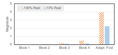
Figure 2: Average distance between the fine-tuned model and a CLIP pre-trained ResNet50 for each Residual block using TPGM. Under the distance constraints imposed by TPGM, most of the model changes are in the last adaptive pooling layer.

TPGM adjusts to the size of training data. As an automatic regularization method, TPGM also needs to adjust to different regularization strengths according to the size of the training set. TPGM can avoid over-fitting to a small fine-tuning dataset through the outer minimization loop of the projection parameters on validation data (Eq. 2). In this section, we additionally present results when we reduce the DomainNet-Real data to 10$\%$ of its original size. We follow a similar strategy as in the $100\%$ experiments and sweep different learning rates (for competing methods we sweep their hyperparameters). All models are trained for 150 epochs. In Tab. 3, we observe significant degradation in ID performance across all methods except for PF and TPGM. PF only trains the Batch-norm layers and therefore is less prone to over-fitting. TPGM achieves an even higher ID performance because it learns small projection radii, which project the fine-tuned model closer to the pre-trained model. To see it, we visualize the average distance between the fined-tuned model and the pre-trained model for each residual block using TPGM for both 100$\%$ and $10\%$ data in Fig. 2. We observe that 1) lower layers have smaller constraints and higher layers have larger constraints, meaning more freedom to grow, and 2) with only $10\%$ training data, the learned constraints are much smaller than those trained with 100$\%$. This behavior explains why TPGM maintains high ID performance and avoids over-fitting with fewer training data because it chooses to rely more on the pre-trained model by enforcing stronger projection.

4.2 Fine-tuning a Pre-Trained Transformer

In this section, we compare to existing fine-tuning methods using a CLIP pre-trained ViT-B model. We initialize all models with the pre-trained weights and also the last linear classifier layer with a zero-shot classifier extracted from the CLIP text-encoder. Specifically, for TPGM, we use $f_{proj}=T-1$ and $T_{proj}=200$, meaning that projection only happens once at the end of fine-tuning. This is possible because CLIP pre-trained ViT-B has been shown to have good linear connectivity [41] in contrast to the CLIP pre-trained ResNet (Appendix 5.7). Furthermore, we use L2 projection in Eq. 3 because we found L2 projection is better than MARS projection in this setting (Appendix 5.6). Training Transformers [37] requires careful tuning of the training recipe to achieve the best results. We follow some common practices in prior works [34, 35] to boost performance. We leave implementation details in Appendix 5.4.

Extracting a Zero-Shot Classifier. CLIP has an image-encoder $g(\cdot)$ and a text-encoder $h(\cdot)$, and is capable of zero-shot classification. For example, given an image $x$ and its label space $y\in\mathcal{Y}=\{y_{1},...,y_{c}\}$, zero-shot classification can be done by first inserting the class name $y_{i}$, e.g., ”apple”, into a template $c_{i}$, e.g., ”a photo of $\{$apple$\}$” and extracting its text embedding $h(c_{i})$, and then computing an inner product,$\langle h(c_{i}),g(x)\rangle$, between the text embedding and the corresponding image embedding. The maximum value of the inner product over all classes determines the membership of the input. Following the prior work [41], one can stack $h(c_{i}),\quad\forall i\in\{1,...,c\}$ into a weight matrix $\mathbf{W}_{\text{zero-shot}}$ as a zero-shot classification layer. We use this weight matrix as initialization as well as zero-shot classification.

Table 4: ImageNet Results using CLIP pre-trained ViT-B. TPGM improves OOD performance significantly without losing ID performance. TPGM-C achieves the best OOD performance while maintaining a more competitive ID performance compared to the current state-of-the-art method WISE. TPGM-C is a controlled variant of TPGM, designed to lower its ID performance to the same level as WISE for a fair comparison of OOD performance. Note that prior works [41] sub-sample classes for ImageNet-A/R (200 classes) for evaluation while we do not.

	ID		OOD			Statistics
	ImageNet	ImageNet-V2	ImageNet-A	ImageNet-R	ImageNet-S	ID Avg.	OOD Avg.	ID $\Delta$ ($\%$)	OOD $\Delta$ ($\%$)
Vanilla FT	84.20 (0.02)	75.08 (0.11)	26.52 (0.12)	46.45 (0.06)	48.90 (0.58)	79.64	40.63	0.00	0.00
LP	77.99 (0.02)	67.74 (0.04)	27.13 (0.06)	50.71 (0.07)	46.47 (0.04)	72.86	41.44	-8.51	2.00
BitFit [48]	78.02 (0.12)	67.69 (0.15)	27.19 (0.28)	50.66 (0.31)	46.50 (0.29)	72.85	41.45	-8.42	2.45
L2-SP [44]	84.10 (0.02)	75.05 (0.11)	26.19 (0.45)	46.58 (0.09)	48.51 (0.12)	79.58	40.43	-0.08	-0.49
LP-FT [21]	83.50 (0.15)	73.95 (0.12)	25.62 (0.23)	46.21 (0.22)	48.83 (0.19)	78.73	40.22	-1.15	-1.00
Zero-Shot [28]	67.68 (N/A)	61.41 (N/A)	30.60 (N/A)	56.77 (N/A)	45.53 (N/A)	64.54	44.30	-18.91	8.64
WISE [41]	82.11 (0.14)	73.61 (0.13)	36.11 (0.16)	61.77 (0.08)	54.16 (0.07)	77.86	50.68	-2.23	24.75
TPGM-C	82.41 (0.07)	73.91 (0.21)	36.79 (0.14)	62.48 (0.10)	54.91 (0.12)	78.16	51.39	-1.86	26.51
TPGM	84.19 (0.03)	75.41 (1.61)	34.29 (2.11)	57.19 (0.54)	54.38 (0.19)	79.80	48.62	0.20	19.69

TPGM Improves OOD robustness without sacrificing ID performance. Now, we present the main benchmark results, accuracy on each of the datasets, and percentage of improvement with respect to the vanilla FT method, in Tab. 4. Parameter-efficient methods such as LP and BitFit all improve OOD generalization however at a loss of ID performance. We hypothesize that they help preserve generalization by updating fewer parameters in the network, and therefore maintaining a closer distance to the pre-trained model. On the other hand, the restriction on the function space can result in under-fitting, manifested in lower ID performance. Surprisingly, L2-SP and LP-FT fail to improve either ID or OOD performance. We think this is because the added regularization in L2-SP and the two-stage training procedure in LP-FT are not very compatible with the existing Transformer training recipe. The zero-shot classifier brings significant OOD improvement even though the ID performance is way worse than the FT model. This confirms that CLIP models acquire great generalization capability during pre-training, as also reported by the original paper [28]. TPGM and WISE perform notably better than other methods. We will elaborate on the comparison next.

TPGM outperforms WISE. The current state-of-the-art method for fine-tuning a pre-trained model with linear connectivity is WISE [41], which linearly interpolates between a fine-tuned model and the pre-trained model with a single ratio. For lack of a better heuristic, the paper suggests 0.5 as the interpolation ratio and leaves the research for a better method to determine the mixing ratio as an open question. The comparison between TPGM and WISE comes down to the comparison between optimized per-layer constraints and a hand-tuned single constraint. Therefore, for WISE, we sweep different ratios from 0.1 to 0.9, controlling the distance to the pre-trained model from close to far. For TPGM, to fairly compare to WISE, we put an L2 regularization on the magnitude of the trainable projection parameters with a hyperparameter $\mu$ that controls the strength of regularization. Intuitively, a larger regularization forces the projection radii to be smaller, meaning projecting the fine-tuned model closer to the pre-trained model. We sweep a range of different $\mu$ from $4e^{-3}$ to $0.0$. We refer to this variant as TPGM-C (C for controlled). Note that this L2 regularization is not a hyper-parameter in the algorithm itself. In Fig. 3, we observe a trade-off between the ID performance and the OOD performance for both methods. However, TPGM clearly outperforms WISE because for the same ID performance, TPGM has better OOD performance and for the same OOD performance, TPGM has better ID performance. This demonstrates the benefits of maintaining per-layer constraints over a single interpolation ratio. We also provide the same experiment and visualization using a CLIP pre-trained ViT-L in Appendix 5.5.

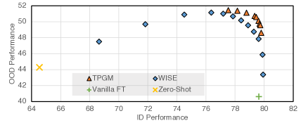
Figure 3: ID and OOD performance of TPGM and WISE with different hyperparameters using CLIP pre-trained ViT-B, fine-tuned on ImageNet. Sweeping different hyperparameters for both WISE and TPGM shows that learning per-layer constraints is superior to learning a single constraint.

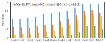
Figure 4: Average distance between the fine-tuned model and a CLIP pre-trained ViT-B for each block using TPGM. Compared to the original distance learned by Vanilla FT, TPGM more aggressively constrains the distance of lower layers.

Different layers require different regularization. Now we take a closer look at the learned TPGM projection radii especially in terms of “closeness” to the pre-trained model. In Fig. 4, we visualize the average distance from the pre-trained model for each transformer block with three different L2 regularization strengths. We observe that 1) lower layers have smaller projection radii, i.e., they are more tightly constrained whereas higher layers have larger projection radii and therefore more freedom to grow; 2) as the regularization strength on projection radii increases, on average, they become closer to the pre-trained model while still following the previous observation. Combined with the common belief that lower layers learn more general features and higher layers learn more specialized layers, we hypothesize that lower layers of the pre-trained model are “closer” to the ideal model than higher layers. This observation corroborates with our theoretical analysis (Sec. 3.4) that when the distance between the pre-trained model and the ideal model is small, TPGM favors close projection.

5 Conclusion

Proposing a bi-level constrained minimization formulation of fine-tuning, we develop the trainable projected gradient method (TPGM) to learn a distance constraint for each layer of a neural network for robust fine-tuning, which has not been possible with manual hyper-parameter tuning. Our thorough experiments across several pre-trained models and ID/OOD datasets show that TPGM can better preserve the OOD generalization capability of the pre-trained model with minimal effects on ID performance. The optimized constraints exhibit highly interpretable patterns which corroborate existing findings and strengthen the motivation for per-layer constraints.

Acknowledgements.

This work was partially supported by Meta, ONR grant N00014-18-1-2829, and GTRI.

5.1 Appendix

5.2 Proof of Theorem 1

We provide complete proof of the main theorem. We will first reiterate the notations used in the main paper.

Problem Setup. Let $x\in\mathbb{R}^{d}$ denote an ID data and the corresponding label $y$ is generated by a ground truth linear model $\theta_{*}\in\mathbb{R}^{d}$, i.e., $y=\theta_{*}^{T}x$. To construct the training set, we sample $n$ training data, where $n<d$, and stack the sampled data into a data matrix $\mathbf{X}_{tr}\in\mathbb{R}^{d\times n}$. Accordingly, the labels form a vector $\mathbf{Y}_{tr}=\mathbf{X}_{tr}^{T}\theta_{*}\in\mathbb{R}^{n}$. The training goal is to minimize the empirical loss.

$$\mathcal{L}(\mathbf{X}_{tr},\mathbf{Y}_{tr};\theta)=\|\mathbf{X}_{tr}^{T}\theta-\mathbf{Y}_{tr}\|_{2}$$ (8)

Note that this forms an over-parameterized linear system, i.e., there are more parameters than equations, because $n<d$. This is similar to how modern neural networks are over-parameterized with respect to the data.

Complementary Decomposition using SVD. For the analysis, we make an independence assumption on the data matrix $\mathbf{X}_{tr}$. This assumption exists for notation simplicity and can be relaxed easily.

Assumption 2.

Let the $n$ training data be linearly independent. The following SVD exists for the data matrix $\mathbf{X}_{tr}$.

$$\mathbf{X}_{tr}=\mathbf{U}\mathbf{\Sigma}\mathbf{V}^{T},\quad\mathbf{U}\in\mathbb{R}^{d\times n},\mathbf{\Sigma}\in\mathbb{R}^{n\times n},\mathbf{V}\in\mathbb{R}^{n\times n}.$$

Consequently, we can decompose any vector $x\in\mathbb{R}^{d}$ into two components, $x=\mathbf{U}\tau+\mathbf{U}_{\bot}\tau_{\bot}$, where $\mathbf{U}$ is the basis for the span of training samples, $\mathbf{U}_{\bot}\in\mathbb{R}^{d\times(d-n)}$ is the basis for the complementary subspace, and $\tau\in\mathbb{R}^{n}$, $\tau_{\bot}\in\mathbb{R}^{d-n}$ are the corresponding coordinates. There are infinitely many solutions to Eq. 8 because this is an over-parameterized system. The classic result states that,

$$\theta=\mathbf{U}\mathbf{\Sigma}^{-1}\mathbf{V}^{T}\mathbf{Y}_{tr}+\mathbf{U}_{\bot}\beta_{\bot},$$ (9)

where $\beta_{\bot}\in\mathbb{R}^{d-n}$ can be any vector. We denote a projected model as $\tilde{\theta}=\theta_{0}+\alpha(\theta-\theta_{0})$ (obtained using Eq. 3 or Eq. 4), where $\theta$ is one minimizer of Eq. 8, $\theta_{0}$ is the pre-trained model and $0\leq\alpha\leq 1$ is the projection ratio.

To quantify the effects of projection $\alpha$, we can look at the average performance of the projected model $\tilde{\theta}$ on test data. Consequently, we investigate the expected loss of the projected model over the entire data space.

$$\mathbb{E}[\mathcal{L}(x,y;\tilde{\theta})]=\mathbb{E}\left[\left\|{\tilde{\theta}}^{T}x-y\right\|_{2}\right]$$ (10)

We now provide a detailed proof of Theorem 1 in the main paper. We first prove two lemmas.

Lemma 1.

$\|(\theta-\theta_{*})^{T}\mathbf{U}\tau\|_{2}=0$.

Proof.

To show it, we use the decomposition in Eq. 9.

$$\|(\theta-\theta_{*})^{T}\mathbf{U}\tau\|_{2} =\|\mathbf{U\Sigma}^{-1}\mathbf{V}^{T}\mathbf{Y}_{tr}+\mathbf{U}_{\bot}\beta_{\bot}-\theta_{*})^{T}\mathbf{U}\tau\|_{2}$$

$$=\|(\mathbf{U\Sigma}^{-1}\mathbf{V}^{T}\mathbf{Y}_{tr}-\theta_{*})^{T}\mathbf{U}\tau\|_{2}$$

$$=\|(\mathbf{U\Sigma}^{-1}\mathbf{V}^{T}\mathbf{X}_{tr}^{T}\theta_{*}-\theta_{*})^{T}\mathbf{U}\tau\|_{2}$$

$$=\|(\mathbf{U\Sigma}^{-1}\mathbf{V}^{T}(\mathbf{U\Sigma V}^{T})^{T}\theta_{*}-\theta_{*})^{T}\mathbf{U}\tau\|_{2}$$

$$=0$$

∎

Lemma 2.

$\|\mathbf{U}\tau\|_{2}\leq\|\tau\|_{2}$ and $\|\mathbf{U}_{\bot}\tau_{\bot}\|_{2}\leq\|\tau_{\bot}\|_{2}$.

Proof.

We first invoke the definition of matrix norm,

$$\|\mathbf{U}\|_{2}=\sup_{\tau\neq 0}\frac{\|\mathbf{U}\tau\|_{2}}{\|\tau\|_{2}}$$

From the definition, it is easy to see that

$$\|\mathbf{U}\tau\|_{2}\leq\|\mathbf{U}\|_{2}\|\tau\|_{2}.$$

Now recall that both $\mathbf{U}\in\mathbb{R}^{d\times n}$ and $\mathbf{U}_{\bot}\in\mathbb{R}^{d\times(d-n)}$ are orthonormal matrices. Therefore, using the property of L2 matrix norm,

$$\|\mathbf{U}\|_{2}=\sqrt{\lambda_{max}(\mathbf{U}^{T}\mathbf{U})}=\sigma_{max}(\mathbf{U})=1$$

where $\lambda_{max}(\cdot)$ and $\sigma_{max}(\cdot)$ denote the largest eigenvalue and singular value respectively. Therefore,

$$\|\mathbf{U}\tau\|_{2}\leq\|\tau\|_{2}.$$

The same analysis extends to $\mathbf{U}_{\bot},\tau_{\bot}$. ∎

Next, we proceed with the proof of the main theorem.

Proof.

$$\mathcal{L}(x,y;\tilde{\theta}) =\left\|{\tilde{\theta}}^{T}x-y\right\|_{2}$$

$$=\left\|(\theta_{0}+\alpha(\theta-\theta_{0}))^{T}x-\theta_{*}^{T}x\right\|_{2}$$

$$=\|(\theta_{0}+\alpha(\theta-\theta_{0})-\theta_{*})^{T}\mathbf{U}\tau+$$

$$(\theta_{0}+\alpha(\theta-\theta_{0})-\theta_{*})^{T}\mathbf{U}_{\bot}\tau_{\bot}\|_{2}$$

$$\leq\underbrace{\|((1-\alpha)(\theta_{0}-\theta_{*})+\alpha({\theta}-\theta_{*}))^{T}\mathbf{U}\tau\|_{2}}_{A}+$$

$$\underbrace{\|(\theta_{0}-\theta_{*})^{T}\mathbf{U}_{\bot}\tau_{\bot}\|_{2}}_{B}+\underbrace{\|\alpha({\theta}-\theta_{0})^{T}\mathbf{U}_{\bot}\tau_{\bot}\|_{2}}_{C}$$

We use triangle inequality for the last inequality. We can now bound $A$ using Lemma 1, Cauchy-Schwarz inequality and Lemma 2 as

$$\|((1-\alpha) (\theta_{0}-\theta_{*})+\alpha({\theta}-\theta_{*}))^{T}\mathbf{U}\tau\|_{2}$$

$$=(1-\alpha)\|(\theta_{0}-\theta_{*})^{T}\mathbf{U}\tau\|_{2}$$

$$\leq(1-\alpha)\|(\theta_{0}-\theta_{*})\|_{2}\|\mathbf{U}\tau\|_{2}$$

$$\leq(1-\alpha)\|(\theta_{0}-\theta_{*})\|_{2}\|\tau\|_{2}.$$

Similarly, we can bound $B$ using Cauchy-Schwarz inequality and Lemma 2 as

$$\|(\theta_{0}-\theta_{*})^{T}\mathbf{U}_{\bot}\tau_{\bot}\|_{2} \leq\|\theta_{0}-\theta_{*}\|_{2}\|\mathbf{U}_{\bot}\tau_{\bot}\|_{2}$$

$$\leq\|\theta_{0}-\theta_{*}\|_{2}\|\tau_{\bot}\|_{2},$$

and bound $C$ as,

$$\|\alpha({\theta}-\theta_{0})^{T}\mathbf{U}_{\bot}\tau_{\bot}\|_{2} \leq\|\alpha({\theta}-\theta_{0})\|_{2}\mathbf{U}_{\bot}\tau_{\bot}\|_{2}$$

$$\leq\|\alpha({\theta}-\theta_{0})\|_{2}\|\tau_{\bot}\|_{2}.$$

Now, plug everything back. We arrive at the final result,

$$\mathcal{L}(x,y;\tilde{\theta})\leq(1-\alpha)\epsilon\|\tau\|_{2}+(\epsilon+\alpha\|\theta-\theta_{0}\|_{2})\|\tau_{\bot}\|_{2}$$

where $\epsilon=\|(\theta_{0}-\theta_{*})\|_{2}$. ∎

5.3 Group Based Total Variation Smoothing

Because of the iterative and incremental nature, the vanilla TPGM algorithm is a greedy algorithm, meaning that it judges the immediate benefit of the current updates to the model weights. If the current updates are not consistent with the validation data, they will be removed by projection, i.e., the projection radii will not increase to accommodate the new changes. Consequently, projection radii learned by TPGM could be overly conservative and lead to underfitting because gradient updates are stochastic, whose benefits may only show up in the long run. Empirically, we found TPGM results in under-fitting in some cases, i.e., slightly lower ID performance. To mitigate this side-effect of iterative optimization, we propose a group-based total variation (TV) smoothing for the projection parameters. TV is a common technique to improve smoothness in image denoising [1] and general signal processing [3]. We propose to utilize TV regularization to enforce a heuristic on the optimization of $\gamma$: projection ratios of layers in the same group should be similar to each other. Specifically, modern neural network architectures such as ResNet [14] and Transformer [37] are modular and stacked with groups (blocks). It is easy to identify unique groups in each architecture and assign layers to each one of them. Therefore, let $\mathcal{G}=\{g_{i}|i=0,...,M\}$ be the set of unique groups in a neural network. The loss function that we optimize for the projection parameters is updated as the following,

$$\mathcal{L}_{\gamma}=\mathcal{L}(x,y;\gamma_{t})+\mu\sum_{g_{i}\in\mathcal{G}}\sum_{i\in g_{i}}|\alpha_{i}-\alpha_{i-1}|$$ (11)

where $\mu$ is a hyperparameter requiring tuning.

5.4 Implementation

In Alg. 2, the projection update function has its own optimizer. In our implementation, we use the Adam [20] optimizer because of its capability of adapting learning rate. Even though this introduces other hyperparameters, we find the same set of hyperparameters worked well for all experiments. Specifically, we use the default settings and a constant base learning rate of $\zeta=1e-2$.

ResNet experiments (Sec. 4.1). We list all the compared methods and their method-specific tuning to reproduce our results.

• Vanilla Fine-Tuning (FT): We fine-tune all layers and sweep five learning rates (CLIP best $\eta_{0}=1e-3$, MOCO best $\eta_{0}=5e-2$).

• Linear Probing (LP): We only fine-tune the head classifier and sweep five learning rates (CLIP best $\eta_{0}=1e-1$, MOCO best $\eta_{0}=1e-1$).

• Partial Fusion (PF) [19]: We fine-tune all the batch-norm layers and the head classifier, and sweep five learning rates (CLIP best $\eta_{0}=1e-2$, MOCO best $\eta_{0}=5e-2$).

• L2-SP [44]: We add L2-SP regularization, use the best-validated learning rate from FT, and sweep five three regularization hyperparameters (CLIP best $\mu:1e-2$, MOCO best $\mu:1e-3$).

• MARS-SP [9]: We add MARS projection (Eq 4), use the best-validated learning rate from FT, and sweep five three projection hyperparameters (CLIP best $\mu=64$, MOCO best $\mu=16$).

• LP-FT [21]: We first LP for 25 epochs, using the best LP learning rate, and FT for another 25 epochs, sweeping five learning rates (CLIP best $\eta_{0}=1e-3$, MOCO best $\eta_{0}=5e-2$).

• TPGM: We learn per-layer L2 projection radii incrementally, sweeping five learning rates (Eq. 3) (CLIP best $\eta_{0}=1e-2$, MOCO best w/o smoothing $\eta_{0}=1e-2$, MOCO w/ smoothing best :$\eta_{0}=4e-2$ and $\mu=0.1$).

Transformer Experiments (Sec. 4.2). We follow some common practices used in prior works [34, 35] to boost fine-tuning performance. Note that we use the same training recipe for all methods unless otherwise specified. For example, linear probing performs worse when augmentations are used [28]. Now we will list the techniques used as well as their corresponding hyperparameters in parenthesis. Specifically, we use label-smoothing ($0.1$) [32], weight-decay ($0.1$), Mixup ($0.8$) [49] and Cutmix ($1.0$) [47]. We fine-tune models using the AdamW optimizer [24] for 30 epochs with a warm-up period of 5 epochs [34], per-step cosine decay schedule [12] and a batch size of $512$. We list all the compared methods and their method-specific tuning to reproduce our results.

• Vanilla Fine-Tuning (FT): We fine-tune all layers and sweep three learning rate $\eta_{0}\in\{1e-5,2e-5,3e-5\}$.

• Linear Probing (LP): We only fine-tune the head classifier and sweep three learning rates $\eta_{0}\in\{5e-2,1e-2,5e-3\}$. We don’t use any data augmentations (e.g., label-smoothing, Mixup and Cutmix) as they decrease LP performance.

• BitFit [48]: We fine-tune all the bias terms and the head classifier and sweep three learning rate $\eta_{0}\in\{5e-2,1e-2,5e-3\}$.

• L2-SP [44]: We add L2-SP regularization, use the best-validated learning rate from FT, and sweep three three regularization hyperparameters $\mu\in\{1e-5,1e-4,1e-3\}$.

• LP-FT [21]: We first LP for 15 epochs, sweeping three learning rates $\eta_{0}\in\{5e-2,1e-2,5e-3\}$, and FT the best-validated model for another 15 epochs, sweeping three learning rate $\eta_{0}\in\{1e-5,2e-5,3e-5\}$.

• Zero-Shot [28]: We run an inference with the pre-trained CLIP model with the extracted zero-shot classifier.

• WISE [41]: We linearly interpolate the best validated FT model and the pre-trained model with a ratio of $0.5$.

• TPGM: We learn per-layer projection radii between the best validated FT model and the pre-trained model using the MARS projection (Eq. 4).

5.5 CLIP Pre-trained ViT-L on ImageNet

In Sec. 4.2, we presented fine-tuning results on ImageNet using CLIP pre-trained ViT-b. In this section, we conduct the same experiments with CLIP pre-trained ViT-L. As we noticed in the ViT-b experiments, WISE and TPGM perform much better than other competitors, so we focus on the comparison between the two here. We first present tabulated results in Tab. 5. We observe that TPGM improves both ID and OOD performance over vanilla FT. To compare fairly with WISE, we introduced TPGM-C (Sec. 4.2), which uses an L2 regularization on the learned projection radii to control the distance to the pre-trained model. With proper regularization, TPGM-C outperforms WISE on both ID and OOD performance. We also provide a figure of ID vs. OOD performance with different WISE interpolation ratios and different TPGM-C regularization strengths in Fig. 5. We observe the same trend as in the ViT-b experiments (Sec. 4.2): at the same ID performance, TPGM has better OOD performance.

Table 5: ImageNet Results using CLIP pre-trained ViT-L. TPGM improves OOD performance significantly without losing ID performance. TPGM-C achieves the best OOD performance while maintaining a more competitive ID performance compared to the current state-of-the-art method WISE. TPGM-C is a controlled variant of TPGM, designed to lower its ID performance to the same level as WISE for a fair comparison of OOD performance.

	ID		OOD			Statistics
	ImageNet	ImageNet-V2	ImageNet-A	ImageNet-R	ImageNet-S	ID Avg.	OOD Avg.	ID $\Delta$ ($\%$)	OOD $\Delta$ ($\%$)
Vanilla FT	87.24	79.25	49.67	63.29	61.62	83.25	58.19	0.00	0.00
Zero-Shot [28]	75.00	69.95	52.21	71.69	58.24	72.48	60.71	-12.94	4.33
WISE [41]	85.33	78.50	58.26	75.37	64.84	81.92	66.16	-1.60	13.68
TPGM-C	86.02	78.83	59.29	76.32	65.00	82.43	66.87	-0.99	14.91
TPGM	87.00	79.81	58.31	74.41	65.13	83.41	65.95	0.19	13.33

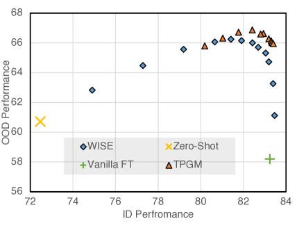
Figure 5: ID and OOD performance of TPGM and WISE with different hyperparameters using CLIP pre-trained ViT-L, fine-tuned on ImageNet. Sweeping different hyperparameters for both WISE and TPGM shows that learning per-layer constraints is superior to learning a single constraint.

5.6 Comparisons between TPGM-L2 and TPGM-MARS

In the main paper, we presented two possible projections: L2 projection (Eq. 3) and MARS projection (Eq. 4). Both projections provide closed-form solutions. We can use either of them in TPGM. In this section, we present comparisons between the two.

Table 6: Comparison between MARS and L2 projections on DomainNet using ResNet50.

		ID	OOD				Statistics
		Real	Sketch	Painting	Infograph	Clipart	OOD Avg.
CLIP	MARS	83.64	38.78	43.11	28.70	48.01	39.65
	L2	82.72	37.18	43.33	25.99	45.71	38.05
MOCO	MARS	81.66	35.97	46.68	20.34	46.11	37.27
	L2	81.66	33.96	45.82	18.71	44.45	35.74

ResNet Experiments on DomainNet. For ResNet experiment in Sec. 4.1, we use a CLIP pre-trained ResNet50 and an ImageNet pre-trained ResNet50. For TPGM, we use $f_{proj}=1$ and $T_{proj}=1$. In Tab. 6, we compare the performance of TPGM using MARS and L2 projections on DomainNet-Real with $100\%$ of its data. We observe that in this setting MARS performs better than L2 projection.

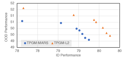
Figure 6: Comparison between MARS and L2 projections on ImageNet using ViT-B.

Transformer Experiments on ImageNet. For Transformer experiments in Sec. 4.2, we use a CLIP pre-trained ViT-B. For TPGM, we use $f_{proj}=T-1$ and $T_{proj}=200$. Following the main paper, we add L2 regularization to the projection radii and sweep a range of values from $4e-3$ to $1e-4$. In Fig. 6, we compare the performance of TPGM using MARS and L2 projections on ImageNet ID and OOD datasets. We observe that L2 projection always outperforms MARS projection in this setting.

5.7 WISE for CLIP Pre-trained ResNet

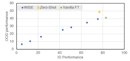
Figure 7: WISE interpolation ratio sweeping using CLIP pre-trained ResNet50 on DomainNet.

The prior work [41] and our experiments in Sec. 4.2 verified that CLIP pre-trained Transformers have very good linear connectivity. This means that when linearly interpolating between the pre-trained model and a fine-tuned model, the output does not degrade much. In this case, we observe significantly improved OOD generalization with minimal ID performance loss. However, the same trend is not observed when switching the architrave to ResNet50. Similar to the prior work [41], we extract a zero-shot classifier for DomainNet classes using a CLIP pre-trained ResNet50 and conduct the same linear interpolation ratio sweeping as in the main paper. In Fig. 7, we plot ID performance against the OOD performance of WISE with different ratios, the pre-trained (zero-shot) model, and the vanilla fine-tuned model. Notably, we observe a significant drop in performance when interpolating between the pre-trained model and a fine-tuned model. This shows that CLIP pre-trained ResNet does not enjoy the same linear connectivity as its Transformer counterpart.

5.8 Smoothing Comparison using MOCO-V3

Table 7: DomainNet Results using MOCO-V3 pre-trained ResNet50 Results with 100$\%$ Real Data. TPGM without TV smoothing achieves the best OOD performance but with slightly worse ID performance compared to vanilla FT. TV smoothing can effectively mitigate this negative effect.

	ID	OOD				Statistics
	Real	Sketch	Painting	Infograph	Clipart	OOD Avg
Vanilla FT	81.99	31.52	42.89	18.51	44.98	34.47
TPGM w/o TV	81.66	35.97	46.68	20.34	46.11	37.27
TPGM w/ TV	82.66	35.35	46.20	20.13	45.75	36.86

In the main paper, we found that training with MOCO-V3 pre-trained ResNet50 on DomainNet can benefit from total variation (TV) smoothing (Appendix 5.3). Here we show a detailed comparison between TPGM with and without smoothing for this particular setting in Tab. 7. We observe that TPGM without smoothing achieves the best OOD performance however with a slight decrease in ID performance compared to vanilla FT. This might be caused by the conservative nature of TPGM as discussed in Appendix 5.3. When TV smoothing is added, we observe that TPGM brings improvement to both ID and OOD performance over vanilla FT.

5.9 Computation Overhead

TPGM inevitably adds some computation overhead to a vanilla fine-tuning pipeline (though not inference). The majority of computation cost comes in Alg. 2, where the algorithm needs to conduct gradient updates on the projection parameters. While this overhead is negligible when we set $f_{freq}=T-1$, i.e., projection update is only called once at the end of training as in the Transformer experiments (Sec. 4.2), the overhead increases when $f_{freq}=1$. In our ResNet experiments (Sec. 4.1), to decrease computation cost, we only the update projection parameters once during each call, i.e, $T_{proj}=1$. Qualitatively, we see an increase of training time from $\sim 29$ hours to $\sim 34$ hours when TPGM is added, a $\sim 17\%$ increase. However, this increase can be justified by the fact that manually searching for per-layer constraints can be intractable.

References

- [1] Qiang Chen, Philippe Montesinos, Quan Sen Sun, Peng Ann Heng, et al. Adaptive total variation denoising based on difference curvature. Image and vision computing, 28(3):298–306, 2010.
- [2] Xinlei Chen, Saining Xie, and Kaiming He. An empirical study of training self-supervised vision transformers. In Proceedings of the IEEE/CVF International Conference on Computer Vision, pages 9640–9649, 2021.
- [3] Laurent Condat. A direct algorithm for 1-d total variation denoising. IEEE Signal Processing Letters, 20(11):1054–1057, 2013.
- [4] Jia Deng, Wei Dong, Richard Socher, Li-Jia Li, Kai Li, and Li Fei-Fei. Imagenet: A large-scale hierarchical image database. In 2009 IEEE conference on computer vision and pattern recognition, pages 248–255. Ieee, 2009.
- [5] Terrance DeVries and Graham W Taylor. Learning confidence for out-of-distribution detection in neural networks. arXiv preprint arXiv:1802.04865, 2018.
- [6] Simon S Du, Wei Hu, Sham M Kakade, Jason D Lee, and Qi Lei. Few-shot learning via learning the representation, provably. arXiv preprint arXiv:2002.09434, 2020.
- [7] Jonathan Frankle, Gintare Karolina Dziugaite, Daniel Roy, and Michael Carbin. Linear mode connectivity and the lottery ticket hypothesis. In International Conference on Machine Learning, pages 3259–3269. PMLR, 2020.
- [8] Jonathan Godwin, Michael Schaarschmidt, Alexander L Gaunt, Alvaro Sanchez-Gonzalez, Yulia Rubanova, Petar Veličković, James Kirkpatrick, and Peter Battaglia. Simple gnn regularisation for 3d molecular property prediction and beyond. In International conference on learning representations, 2021.
- [9] Henry Gouk, Timothy M Hospedales, and Massimiliano Pontil. Distance-based regularisation of deep networks for fine-tuning. ICLR, 2021.
- [10] Chuan Guo, Geoff Pleiss, Yu Sun, and Kilian Q Weinberger. On calibration of modern neural networks. In International conference on machine learning, pages 1321–1330. PMLR, 2017.
- [11] Yunhui Guo, Honghui Shi, Abhishek Kumar, Kristen Grauman, Tajana Rosing, and Rogerio Feris. Spottune: transfer learning through adaptive fine-tuning. In Proceedings of the IEEE/CVF conference on computer vision and pattern recognition, pages 4805–4814, 2019.
- [12] Kaiming He, Xinlei Chen, Saining Xie, Yanghao Li, Piotr Dollár, and Ross Girshick. Masked autoencoders are scalable vision learners. In Proceedings of the IEEE/CVF Conference on Computer Vision and Pattern Recognition, pages 16000–16009, 2022.
- [13] Kaiming He, Ross Girshick, and Piotr Dollár. Rethinking imagenet pre-training. In Proceedings of the IEEE/CVF International Conference on Computer Vision, pages 4918–4927, 2019.
- [14] Kaiming He, Xiangyu Zhang, Shaoqing Ren, and Jian Sun. Deep residual learning for image recognition. In Proceedings of the IEEE conference on computer vision and pattern recognition, pages 770–778, 2016.
- [15] Dan Hendrycks, Steven Basart, Norman Mu, Saurav Kadavath, Frank Wang, Evan Dorundo, Rahul Desai, Tyler Zhu, Samyak Parajuli, Mike Guo, et al. The many faces of robustness: A critical analysis of out-of-distribution generalization. In Proceedings of the IEEE/CVF International Conference on Computer Vision, pages 8340–8349, 2021.
- [16] Dan Hendrycks, Kimin Lee, and Mantas Mazeika. Using pre-training can improve model robustness and uncertainty. In International Conference on Machine Learning, pages 2712–2721. PMLR, 2019.
- [17] Dan Hendrycks, Kevin Zhao, Steven Basart, Jacob Steinhardt, and Dawn Song. Natural adversarial examples. In Proceedings of the IEEE/CVF Conference on Computer Vision and Pattern Recognition, pages 15262–15271, 2021.
- [18] Alfredo N Iusem. On the convergence properties of the projected gradient method for convex optimization. Computational & Applied Mathematics, 22:37–52, 2003.
- [19] Fahdi Kanavati and Masayuki Tsuneki. Partial transfusion: on the expressive influence of trainable batch norm parameters for transfer learning. In Medical Imaging with Deep Learning, pages 338–353. PMLR, 2021.
- [20] Diederik P Kingma and Jimmy Ba. Adam: A method for stochastic optimization. arXiv preprint arXiv:1412.6980, 2014.
- [21] Ananya Kumar et al. Fine-tuning can distort pretrained features and underperform out-of-distribution. ICLR, 2022.
- [22] Yoonho Lee, Annie S Chen, Fahim Tajwar, Ananya Kumar, Huaxiu Yao, Percy Liang, and Chelsea Finn. Surgical fine-tuning improves adaptation to distribution shifts. arXiv preprint arXiv:2210.11466, 2022.
- [23] Xingjian Li, Haoyi Xiong, Hanchao Wang, Yuxuan Rao, Liping Liu, Zeyu Chen, and Jun Huan. Delta: Deep learning transfer using feature map with attention for convolutional networks. arXiv preprint arXiv:1901.09229, 2019.
- [24] Ilya Loshchilov and Frank Hutter. Decoupled weight decay regularization. arXiv preprint arXiv:1711.05101, 2017.
- [25] Krikamol Muandet, David Balduzzi, and Bernhard Schölkopf. Domain generalization via invariant feature representation. In International Conference on Machine Learning, pages 10–18. PMLR, 2013.
- [26] Behnam Neyshabur, Hanie Sedghi, and Chiyuan Zhang. What is being transferred in transfer learning? Advances in neural information processing systems, 33:512–523, 2020.
- [27] Xingchao Peng, Qinxun Bai, Xide Xia, Zijun Huang, Kate Saenko, and Bo Wang. Moment matching for multi-source domain adaptation. In Proceedings of the IEEE/CVF international conference on computer vision, pages 1406–1415, 2019.
- [28] Alec Radford, Jong Wook Kim, Chris Hallacy, Aditya Ramesh, Gabriel Goh, Sandhini Agarwal, Girish Sastry, Amanda Askell, Pamela Mishkin, Jack Clark, et al. Learning transferable visual models from natural language supervision. In International Conference on Machine Learning, pages 8748–8763. PMLR, 2021.
- [29] Maithra Raghu, Chiyuan Zhang, Jon Kleinberg, and Samy Bengio. Transfusion: Understanding transfer learning for medical imaging. Advances in neural information processing systems, 32, 2019.
- [30] Benjamin Recht, Rebecca Roelofs, Ludwig Schmidt, and Vaishaal Shankar. Do imagenet classifiers generalize to imagenet? In International Conference on Machine Learning, pages 5389–5400. PMLR, 2019.
- [31] Zhiqiang Shen, Zechun Liu, Jie Qin, Marios Savvides, and Kwang-Ting Cheng. Partial is better than all: Revisiting fine-tuning strategy for few-shot learning. In Proceedings of the AAAI Conference on Artificial Intelligence, volume 35, pages 9594–9602, 2021.
- [32] Christian Szegedy, Vincent Vanhoucke, Sergey Ioffe, Jon Shlens, and Zbigniew Wojna. Rethinking the inception architecture for computer vision. In Proceedings of the IEEE conference on computer vision and pattern recognition, pages 2818–2826, 2016.
- [33] Junjiao Tian, Dylan Yung, Yen-Chang Hsu, and Zsolt Kira. A geometric perspective towards neural calibration via sensitivity decomposition. Advances in Neural Information Processing Systems, 34:26358–26369, 2021.
- [34] Hugo Touvron, Matthieu Cord, Matthijs Douze, Francisco Massa, Alexandre Sablayrolles, and Hervé Jégou. Training data-efficient image transformers & distillation through attention. In International Conference on Machine Learning, pages 10347–10357. PMLR, 2021.
- [35] Hugo Touvron, Matthieu Cord, and Hervé Jégou. Deit iii: Revenge of the vit. arXiv preprint arXiv:2204.07118, 2022.
- [36] Nilesh Tripuraneni, Michael Jordan, and Chi Jin. On the theory of transfer learning: The importance of task diversity. Advances in Neural Information Processing Systems, 33:7852–7862, 2020.
- [37] Ashish Vaswani, Noam Shazeer, Niki Parmar, Jakob Uszkoreit, Llion Jones, Aidan N Gomez, Łukasz Kaiser, and Illia Polosukhin. Attention is all you need. Advances in neural information processing systems, 30, 2017.
- [38] Haohan Wang, Songwei Ge, Zachary Lipton, and Eric P Xing. Learning robust global representations by penalizing local predictive power. Advances in Neural Information Processing Systems, 32, 2019.
- [39] Mei Wang and Weihong Deng. Deep visual domain adaptation: A survey. Neurocomputing, 312:135–153, 2018.
- [40] Yang Wen, Leiting Chen, Yu Deng, and Chuan Zhou. Rethinking pre-training on medical imaging. Journal of Visual Communication and Image Representation, 78:103145, 2021.
- [41] Mitchell Wortsman, Gabriel Ilharco, Jong Wook Kim, Mike Li, Simon Kornblith, Rebecca Roelofs, Raphael Gontijo Lopes, Hannaneh Hajishirzi, Ali Farhadi, Hongseok Namkoong, et al. Robust fine-tuning of zero-shot models. In Proceedings of the IEEE/CVF Conference on Computer Vision and Pattern Recognition, pages 7959–7971, 2022.
- [42] Sen Wu, Hongyang R Zhang, and Christopher Ré. Understanding and improving information transfer in multi-task learning. arXiv preprint arXiv:2005.00944, 2020.
- [43] Sang Michael Xie, Ananya Kumar, Robbie Jones, Fereshte Khani, Tengyu Ma, and Percy Liang. In-n-out: Pre-training and self-training using auxiliary information for out-of-distribution robustness. arXiv preprint arXiv:2012.04550, 2020.
- [44] LI Xuhong, Yves Grandvalet, and Franck Davoine. Explicit inductive bias for transfer learning with convolutional networks. In International Conference on Machine Learning, pages 2825–2834. PMLR, 2018.
- [45] Jason Yosinski, Jeff Clune, Yoshua Bengio, and Hod Lipson. How transferable are features in deep neural networks? Advances in neural information processing systems, 27, 2014.
- [46] Kaichao You, Mingsheng Long, Zhangjie Cao, Jianmin Wang, and Michael I Jordan. Universal domain adaptation. In Proceedings of the IEEE/CVF conference on computer vision and pattern recognition, pages 2720–2729, 2019.
- [47] Sangdoo Yun, Dongyoon Han, Seong Joon Oh, Sanghyuk Chun, Junsuk Choe, and Youngjoon Yoo. Cutmix: Regularization strategy to train strong classifiers with localizable features. In Proceedings of the IEEE/CVF international conference on computer vision, pages 6023–6032, 2019.
- [48] Elad Ben Zaken, Shauli Ravfogel, and Yoav Goldberg. Bitfit: Simple parameter-efficient fine-tuning for transformer-based masked language-models. arXiv preprint arXiv:2106.10199, 2021.
- [49] Hongyi Zhang, Moustapha Cisse, Yann N Dauphin, and David Lopez-Paz. mixup: Beyond empirical risk minimization. arXiv preprint arXiv:1710.09412, 2017.
- [50] Kaiyang Zhou, Ziwei Liu, Yu Qiao, Tao Xiang, and Chen Change Loy. Domain generalization: A survey. IEEE Transactions on Pattern Analysis and Machine Intelligence, 2022.