On the Convergence of Decentralized Federated Learning Under Imperfect Information Sharing

Abstract

Decentralized learning and optimization is a central problem in control that encompasses several existing and emerging applications, such as federated learning. While there exists a vast literature on this topic and most methods centered around the celebrated average-consensus paradigm, less attention has been devoted to scenarios where the communication between the agents may be imperfect. To this end, this paper presents three different algorithms of Decentralized Federated Learning (DFL) in the presence of imperfect information sharing modeled as noisy communication channels. The first algorithm, Federated Noisy Decentralized Learning (FedNDL1), comes from the literature, where the noise is added to their parameters to simulate the scenario of the presence of noisy communication channels. This algorithm shares parameters to form a consensus with the clients based on a communication graph topology through a noisy communication channel. The proposed second algorithm (FedNDL2) is similar to the first algorithm but with added noise to the parameters, and it performs the gossip averaging before the gradient optimization. The proposed third algorithm (FedNDL3), on the other hand, shares the gradients through noisy communication channels instead of the parameters. Theoretical and experimental results demonstrate that under imperfect information sharing, the third scheme that mixes gradients is more robust in the presence of a noisy channel compared with the algorithms from the literature that mix the parameters.

I Introduction

Due to technological advances, a massive amount of data is being generated from devices like computers, mobiles, smart watches, and vehicles which are collected in centralized data centers and subsequently used for training machine learning models. However, challenges such as limited communication bandwidth, memory constraints, and privacy concerns make centralized learning not reliable and scalable. Hence, learning paradigms that promote a secure and privacy-preserving environment must be created. This led to an advancement in decentralized optimization algorithms [1, 2] such as the Decentralized Federated Learning (DFL) [3] and Federated Learning (FL)[4, 5] where only weights or gradients are transferred instead of the raw data from all agents involved. FL, in particular, is a new technique developed to address these issues specifically and has found applications in several domains like hospitals, mobile mobiles, and connected vehicles [6, 7, 8].

I-A Related work

A canonical approach to decentralized optimization is consensus-based gradient descent methods [9, 1, 10, 11] which compute local weights and gradients for all clients’ local data and then share the computed parameters with other clients. The weight/gradient is then averaged from all the clients based on a network topology that dictates the communication structure of the learning paradigm. The network topology can be represented as a simple graph where edges represent communication links with individual clients through which the parameters (weights or gradients) are shared. These decentralized topologies minimize critical bottlenecks of centralized methods, such as network communication latency and network bandwidth, to improve scalability and efficiency in large-scale settings [10, 12].

While communication efficiency is one of the critical elements and challenges for distributed learning, and several efforts, including communication compression, have been made in this regard [13, 14, 15, 16, 3, 17, 18], these methods generally assume that the communication channels are noiseless. The performance of the trained model in the presence of noise should be one of the critical criteria in choosing the machine learning framework to ensure the robustness and safety of emerging applications that rely on distributed learning.

The effect of imperfect information sharing such as noisy communication or quantization noise in an average consensus algorithm in a distributed framework was studied in [19, 20]. However, the impact of various levels of noise has not been studied. Additionally, the study in [19] is limited to consensus problems only and does not encompass unique challenges that arise in modern decentralized optimization and learning, e.g., the inherent non-convexity of the learning objective. Other works including [21, 22, 23, 24, 25, 26] study the impact of noise in server-assisted FL. These works require a server, and they require somewhat restrictive assumptions that typically are not satisfied in practical settings or are hard to verify. Unlike FL, DFL has no central server, and each client, effectively, acts as its own individual server. Here, each client, typically, performs local Stochastic Gradient Descent (SGD) or its variations on its local dataset and exchanges messages only with its immediate neighbors.

In this paper, our primary focus is on DFL in the presence of noise in communication channels. Recently, [27, 28, 29, 30] study the performance of a two-time scale method [31] for DFL with channel noise while requiring the convexity of the objective function, uniformly bounded gradients, and access to the deterministic gradients; note that these three considerations are very restrictive assumptions, especially in emerging settings in large-scale learning.

I-B Contribution

Motivated by the existing gap between perfect information and noisy decentralized learning, in this paper, we model the presence of noise in the communication channels as random vector with zero mean and different variances and study the performance of three decentralized FL algorithms by adding the noise to the parameters. In particular, we study the impact of noise in communication channels in three algorithms. The first algorithm, Federated Noisy Decentralized Learning (FedNDL1) was recently considered in [2], where the parameters were not subjected to any communication noise. In our analysis of this algorithm, we added noise to the parameters after the local SGD update. The new parameter with the noise is then exchanged with other clients through the gossip matrix (communication matrix as per the communication graph), and the global parameters are updated. This iteration, also known as communication rounds, continues throughout the training. In the second algorithm (FedNDL2), which is related to [1], the noise is added before the consensus and local SGD update. In the third algorithm (FedNDL3), which has been considered in the noiseless case in [32], the noise is added to the gradients as opposed to the parameters, and the result is exchanged with the immediate clients.

We demonstrate, theoretically and empirically, that there are benefits in using FedNDL3 in the imperfect information setting that communicates the stochastic gradients. The intuition which is formalized theoretically is that the parameters are sensitive to the added noise while the stochastic gradients, which are already imperfect, are resilient. Therefore, the error stemming from weaker consensus in FedNDL3 is not as severe as the detrimental impact of noise on FedNDL1 and FedNDL2.

II Problem Statement

In this section, we describe the problem structure, assumptions, and the proposed algorithms that we analyzed in this paper. We start with a standard DFL setup in which $n$ clients/agents have their own local datasets and collaborate with each other to update the global parameters. Formally, the problem can be represented as

$$\min_{x\in\mathbb{R}^{d}}\Big{[}f(x)=\frac{1}{n}\sum_{i=1}^{n}f_{i}(x_{i})\Big{]},$$ (1)

where $f_{i}:\mathbb{R}^{d}\to\mathbb{R}$ for $i\in\{1,\dots,n\}$ is the local objective function of the $i^{th}$ client node. The stochastic formulation of the local objective function can be written

$$f_{i}(x)=\operatorname{\mathbb{E}}_{\xi_{i}\sim\mathcal{D}_{i}}[\ell(x_{i},\xi_{i})],$$ (2)

where $\xi_{i}$ is the data that has been sampled from the data distribution $\mathcal{D}_{i}$ for the $i^{th}$ client. The function $\ell(x_{i},\xi_{i})$ is the loss function evaluated for each client and for each data sample $\xi_{i}$. Here $x_{i}\in\mathbb{R}^{d}$ is the parameter vector of client $i$, and $X\in\mathbb{R}^{d\times n}$ is the matrix formed using these parameter vectors. The $i$-th column of this matrix corresponds to the parameter vector of $i$-th client. Thus, the primary objective of the clients is to achieve optimality through collaboration i.e., $x_{i}=x^{*}$.

The main idea of the process is to achieve consensus in which the client can only communicate with its adjacent neighbors. This process of communication can be modeled using a communication graph with the help of a consensus matrix. More precisely, a client $i$ communicates with client $j$ based on a non-negative weight, $w_{ij}>0$, that formulates the connectivity of client $i$ and client $j$. Similarly, for self-loops, the associated weight, $w_{ii}>0$, and $w_{ij}=0$ if there is no communication supposed to happen between $i$ and $j$. These associated weights are then placed in a matrix of dimension $n\times n$ and can be written as $W=[w_{ij}]\in[0,1]^{n\times n}$. The standard name for $W$ in the literature is the gossip or mixing matrix. To proceed, we define the mixing matrix.

Definition 1 (Mixing matrix).

The mixing/gossip matrix, $W=[w_{ij}]\in[0,1]^{n\times n}$, is a non-negative, symmetric $(W=W^{\top})$ and doubly stochastic $(\mathds{1}W=\mathds{1},\mathds{1}^{\top}W=\mathds{1}^{\top})$ matrix, where $\mathds{1}$ is the column vector of unit elements of size $n$

We next describe the algorithms studied in this paper. The entire process of DFL can be viewed as a two-stage pipeline: 1) SGD update step, performed locally on each client, and 2) Gossip/Consensus averaging step. We analyze three different scenarios of noise injection, resulting in three different algorithms.

II-A Algorithm 1—FedNDL1

In this algorithm, each client in parallel performs updates first, see—lines 4–6, and then communicates the updated parameters to their neighbors. The communication depends on the topology of the communication graph, i.e., the mixing matrix, $W$, through a noisy communication channel (line 7). Due to the noisy communication channel, the neighboring client receives a noisy version of the parameters,

$$x_{i}^{(t+1)}\ =\ \sum_{j=1}^{n}w_{ij}\ (x_{j}^{(t+\frac{1}{2})}+\delta_{j}^{(t)}),$$ (3)

where $\delta_{j}^{(t)}\in\mathbb{R}^{d}$, is a zero mean random noise and $x_{j}^{(t+\frac{1}{2})}$ is the vector of parameters sent by client $j$. Since we assume the noise to have a zero mean, the noise variance is

$$D^{2}_{t,j}=\operatorname{\mathbb{E}}[\|\delta_{j}^{(t)}\|^{2}].$$ (4)

II-B Algorithm 2—FedNDL2

Similar to the previous algorithm, this algorithm also performs a two-stage process. However, in this algorithm, we perform the consensus step (line 9) over a noisy communication channel before computing the individual gradients,

$$x_{i}^{(t+\frac{1}{2})}=\sum_{j=1}^{n}w_{ij}(x_{j}^{(t)}+\delta_{j}^{(t)}),$$ (5)

where the symbols hold the same meaning as in the previous one. After the gossip averaging step, each client performs the SGD update on their local data (lines 10–12).

II-C Algorithm 3—FedNDL3

In FedNDL3, the clients share their gradients over a noisy communication channel instead of the weights followed by the SGD update. The reason behind pursuing this idea comes from the motivation for our study of Noisy-FL and the fact that SGD inherently is a noisy process. So, pursuing this scenario gives more flexibility to handle the noise as a part of the SGD process. The entire formulation for this process can be written as,

$$x_{i}^{(t+1)}\ =\ x_{i}^{(t)}-\eta_{t}\sum_{j=1}^{n}w_{ij}\ (g_{j}^{(t)}+\delta_{j}^{(t)}),$$ (6)

where $g_{j}^{(t)}$ refers to a stochastic gradient of client $j$ at iteration $t$ and the rest of the terms hold the same meaning as before. The algorithms are summarized in the table above.

Algorithm FedNDL1, FedNDL2, and FedNDL3

1:  Input: For each node $i$ initialize: $x_{i}^{(0)}\ \in\ \mathbb{R}^{d}$, step size $\{\eta_{t}\}_{t=0}^{T-1}$, mixing matrix $W$, noise from the communication channel $\delta^{(t)}$

2:  for $t=0,\dots,T$ do

3:      FedNDL1:

4:      Run in parallel for each client $i$

5:      Sample $\xi_{i}^{(t)}\mbox{, compute }g_{i}^{(t)}=\widetilde{\nabla}f_{i}(x_{i}^{(t)},\xi_{i}^{(t)})$

6:      $x_{i}^{(t+\frac{1}{2})}\ =\ x_{i}^{(t)}-\eta_{t}g_{i}^{(t)}$ 

7:      $x_{i}^{(t+1)}\ =\ \sum_{j=1}^{n}w_{ij}\ (x_{j}^{(t+\frac{1}{2})}+\delta_{j}^{(t)})$ 

8:      FedNDL2:

9:      $x_{i}^{(t+\frac{1}{2})}\ =\ \sum_{j=1}^{n}w_{ij}\ (x_{j}^{(t)}+\delta_{j}^{(t)})\$

10:      Run in parallel for each clients $i$

11:      Sample $\xi_{i}^{(t)}\mbox{ , }g_{i}^{(t+\frac{1}{2})}=\widetilde{\nabla}f_{i}(x_{i}^{(t+\frac{1}{2})},\xi_{i}^{(t)})$  

12:      $x_{i}^{(t+1)}\ =\ x_{i}^{(t+\frac{1}{2})}-\eta_{t}g_{i}^{(t+\frac{1}{2})}$

13:      FedNDL3:

14:      Run in parallel for each client $i$

15:      Sample $\xi_{i}^{(t)}\mbox{, compute }g_{i}^{(t)}=\widetilde{\nabla}f_{i}(x_{i}^{(t)},\xi_{i}^{(t)})$

16:      $x_{i}^{(t+1)}\ =\ x_{i}^{(t)}-\eta_{t}\sum_{j=1}^{n}w_{ij}\ (g_{j}^{(t)}+\delta_{j}^{(t)})\$

17:  end for

II-D Assumptions

We now discuss the assumptions we made in our analysis of the proposed algorithms. They are standard assumptions used in the study and analysis of distributed and decentralized algorithms, see [33, 2, 3].

Assumption 1 (Smoothness).

The objective function $\ell(x,\xi)$ is $L$-smooth with respect to $x$, for all $\xi$. Each $f_{i}(x)$ is $L$-smooth, that is,

$$\|\nabla f_{i}(x)-\nabla f_{i}(y)\|\leq L\|x-y\|,\qquad\mbox{for all x,y}.$$ (7)

Hence the function $f$ is also $L$-smooth.

Assumption 2 (Bounded Variance).

The variance of the stochastic gradient of each client $i$ is bounded,

$$\operatorname{\mathbb{E}}[||\widetilde{\nabla}f_{i}(x_{i}^{t},\xi_{i}^{t})-\nabla f_{i}(x_{i}^{t})||^{2}]\leq\sigma^{2},$$

where $\xi_{i}^{t}$ denotes random batch of samples in client node $i$ for $t^{th}$ round, and $\widetilde{\nabla}f_{i}(x_{i}^{t},\xi_{i}^{t})$ denotes the stochastic gradient. In addition, we also assume that the stochastic gradient is unbiased, i.e., $\operatorname{\mathbb{E}}[\widetilde{\nabla}(f_{i}(x_{i}^{t},\xi_{i}^{t}))]=\nabla f_{i}(x_{i}^{t})$.

Assumption 3 (Mixing matrix).

The mixing matrix W satisfies for $\rho\in(0,1]$,

$$\|(\bar{X}-X)W\|_{F}^{2}\leq(1-\rho)\|\bar{X}-X\|_{F}^{2},$$

which means that the gossip averaging step brings the columns of $X\in\mathbb{R}^{d\times n}$ closer to the row-wise average, that is, $\bar{X}=X\frac{\mathds{1}\mathds{1}^{\top}}{n}$.

Assumption 4 (Bounded Client Dissimilarity (BCD)).

For all $x\in\mathbb{R}^{d}$,

$$\frac{1}{n}\sum_{i=1}^{n}\|\nabla f_{i}(x)-\nabla f(x)\|^{2}\leq B^{2},$$

where B is a constant.

The above assumption is made to limit the extent of client heterogeneity and is standard in the DFL setup. While methods based on gradient tracking [34] do no require this assumption, they suffer from increased communication cost and the variance, which limits their practicality [35]. Note that this assumption is only used in the analysis of FedNDL1 and FedNDL2.

Assumption 5 (Noise model).

The noise present due to contamination of communication channel $\delta_{i}^{(t)}$ is independent, has zero mean and bounded variance, that is, $\operatorname{\mathbb{E}}[\delta_{i}^{(t)}]=0$ and $\operatorname{\mathbb{E}}[||\delta_{i}^{(t)}||^{2}]=D_{t,i}^{2}<\infty$.

This assumption is specific to the imperfect information sharing setup and is considered recently in [29, 30, 26].

Assumption 6 (Bounded Recursive Consensus Error).

Let the consensus error be defined as $(C.E)_{t}=\frac{1}{n}\|\bar{X}_{t}-{X}_{t}\|^{2}_{F}$. We assume that the consensus error is upper bounded,

$$\operatorname{\mathbb{E}}[(C.E)_{t+1}]\leq\rho_{t}\operatorname{\mathbb{E}}[(C.E)_{t}]+\gamma_{t},$$

where $\rho_{t}\in(0,1)$ and $\gamma_{t}\geq 0$.

Remark.

We use this assumption in the convergence analysis of FedNDL3. Theoretically speaking the above assumption 6 can be viewed as a general formulation one obtains while unfolding the recursion of consensus error in the analysis of decentralized SGD—see, e.g., [2]. Additionally, this assumption is satisfied by FedNDL1 and FedNDL2 with $\rho_{t}=\rho$ and certain $\{\gamma_{t}\}$ that depends on other parameters of the problem. We further note that using multi-round gossiping [3] or acceleration methods such as Chebyshev acceleration [36, 37] this assumption may be satisfied by FedNDL3 as well and $\rho_{t}$ and $\gamma_{t}$ can be significantly reduced.

III Convergence Analysis

In this section, we state the main theorem providing an upper bound on the convergence error of FedNDL1, FedNDL2 and FedNDL3. The convergence results for all the algorithms are for a non-convex $L$-smooth loss function. These results are for the case when there is noise present due to the imperfection of the communication channel,

Theorem 1 (Smooth non-convex cases for Noisy-DFL).

Suppose Assumptions 1, 2, 3, 4, 5 and 6 (only for FedNDL3) hold. Let $\eta L<\frac{1}{12}$, $\eta=\mathcal{O}(\frac{1}{\sqrt{T}})$ and $\bar{D}^{2}=\frac{1}{nT}\sum_{t,i=1,1}^{T,n}D^{2}_{t,i}$, then we have:

• FedNDL1: For $\eta L<\frac{\rho}{2\sqrt{6}}$,

  $$\frac{1}{T}\sum_{t=1}^{T}\operatorname{\mathbb{E}}[\|\nabla f(\bar{x}_{t})\|^{2}]+\frac{L^{2}}{T}\sum_{t=1}^{T}\operatorname{\mathbb{E}}[(C.E)_{t}]=\mathcal{O}\Big{(}\frac{\rho}{n\sqrt{T}}\sigma^{2}+\frac{\rho^{2}}{T}B^{2}+\frac{T^{\frac{3}{2}}}{\rho}\bar{D}^{2}\Big{)},$$ (8)

• FedNDL2: For $\eta L<\frac{\rho}{4\sqrt{3}}$,

  $$\frac{1}{T}\sum_{t=1}^{T}\operatorname{\mathbb{E}}[\|\nabla f(\bar{x}_{t})\|^{2}]+\frac{L^{2}}{T}\sum_{t=1}^{T}\operatorname{\mathbb{E}}[(C.E)_{t}]=\mathcal{O}\Big{(}\frac{\rho}{n\sqrt{T}}\sigma^{2}+\frac{\rho^{2}}{T}B^{2}+\frac{T^{\frac{3}{2}}}{\rho}\bar{D}^{2}\Big{)},$$ (9)

• FedNDL3:

  $$\frac{1}{T}\sum_{t=1}^{T}\operatorname{\mathbb{E}}[\|\nabla f(\bar{x}_{t})\|^{2}]+\frac{L^{2}}{T}\sum_{t=1}^{T}\operatorname{\mathbb{E}}[(C.E)_{t}]=\mathcal{O}\Big{(}\frac{1}{n\sqrt{T}}\sigma^{2}+\frac{1}{T}\sum_{t=1}^{T}\frac{\gamma_{t}}{\rho_{t}}+\frac{1}{\sqrt{T}}\bar{D}^{2}\Big{)},$$ (10)

where all expectations are w.r.t. the data and the noise.

Theorem 1 establishes a worst-case upper bound on the convergence of the three algorithms studied in the paper. In particular, the theorem jointly bounds the expected gradient norm (which is a notion of approximate first-order stationarity of the average iterate $\bar{x}_{t}$) and the consensus error. The convergence bounds consist of three terms: the first term effectively captures the error arising from inaccurate initialization and stochasticity of the first-order oracle, which matches the error of centralized SGD. The second term captures the effect of data heterogeneity, and the last term captures the adverse effect of imperfect communication modeled as communication noise.

In addition, Theorem 1 captures the impact of presence channel noise on the convergence of studied algorithms. Specifically, (8) and (9) indicate that FedNDL1 and FedNDL2 suffer from a severe impact of noise on the worst-case convergence: as the number of communication rounds/iterations $T$ increases the guarantee on finding a stationary solution and consensus error weakens. In fact, the error increases with $T$. We will verify these results further numerically in Section IV. Furthermore, as the connectivity of the communication graphs decreases (which corresponds to a smaller $\rho$), the impact of noise increases. This point is further verified in Section IV. With regard to FedNDL3, however, Theorem 1 establishes that the algorithm is resilient to the impact of noise. In particular, in contrast with the convergence bound of FedNDL1 and FedNDL2, the last term in (10) decreases with $T$. Intuitively, this theoretically-grounded property is linked to SGD which inherently is a noisy process and thus is more resilient towards added noise to a certain degree. Theorem 1 further shows that, different from FedNDL1 and FedNDL2, the impact of noise is independent of the communication topology as the last term in (10) is independent of $\rho_{t}$ and $\gamma_{t}$. In Section IV we numerically verify these two distinguishing properties of FedNDL3.

III-A Proof-Sketch

e start the proof by upper bounding the second moment of the gradient on the average of iterates by using the $L$-smoothness of the loss function. This step is a standard practice used in the convergence proofs for non-convex, $L$-smooth loss functions. The second moment here is bounded by the inaccurate initialization, the variance of the stochastic gradients, noise present due to imperfect channels, and the consensus error function, $(C.E)_{t}$. For FedNDL3, in the next step, we proceed with upper bounding the $(C.E)_{t+1}$ followed by defining a potential function,

$$\psi_{t}=\operatorname{\mathbb{E}}[f(\bar{x}_{t})]+\phi(C.E)_{t},{\text{ where $\phi>0$ is a constant.}}$$ (11)

This new potential function enables us to jointly bound the expected gradient norm and the consensus error without requiring restrictive and impractical assumptions such as the bounded gradient norm assumption. Another noteworthy point here is the term $\phi$ for FedNDL3 which now, unlike in (11), is time-dependent and is denoted as $\phi_{t}$. Now, we telescope over the $\psi_{t+1}-\psi_{t}$ for $t=\{1,\ldots,T\}$ and dividing it by $T$, along with specific choices of $\phi$ and $\phi_{t}$ results in Theorem 1. Detailed proofs for FedNDL1, FedNDL2 and FedNDL3 are provided in the

(a) Fully-connected topology

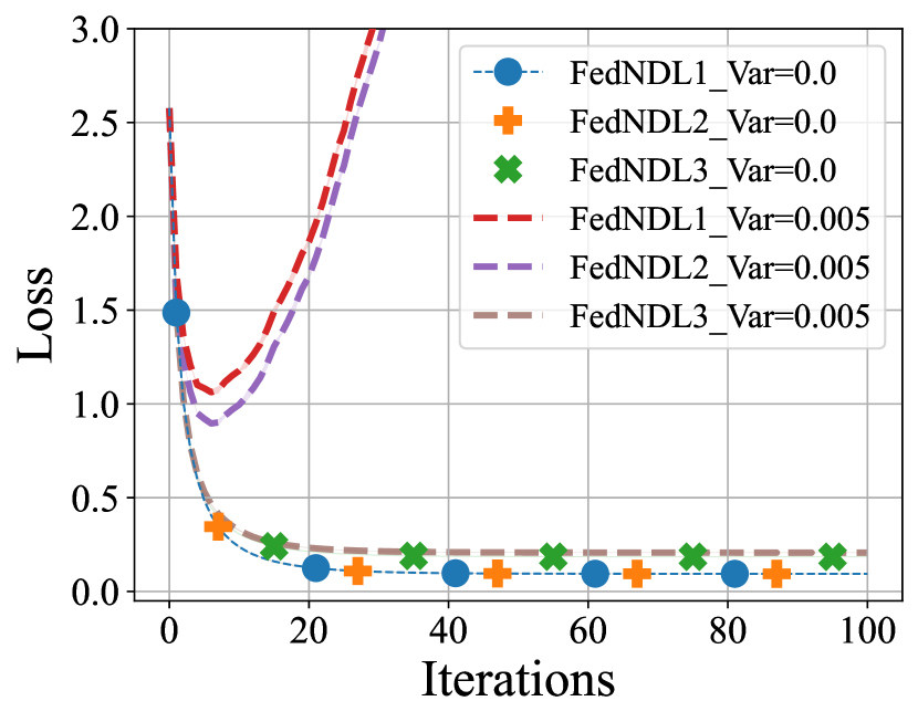
(b) Torus topology

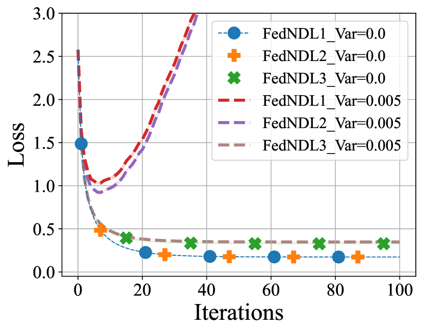
(c) Ring topology

Figure 1: Loss vs. iterations with and without noise for different communication topologies.

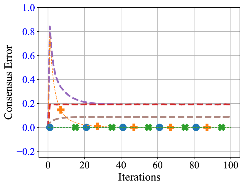
(a) Fully-connected topology

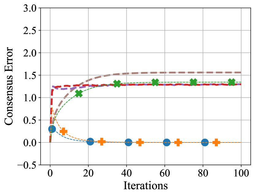
(b) Torus topology

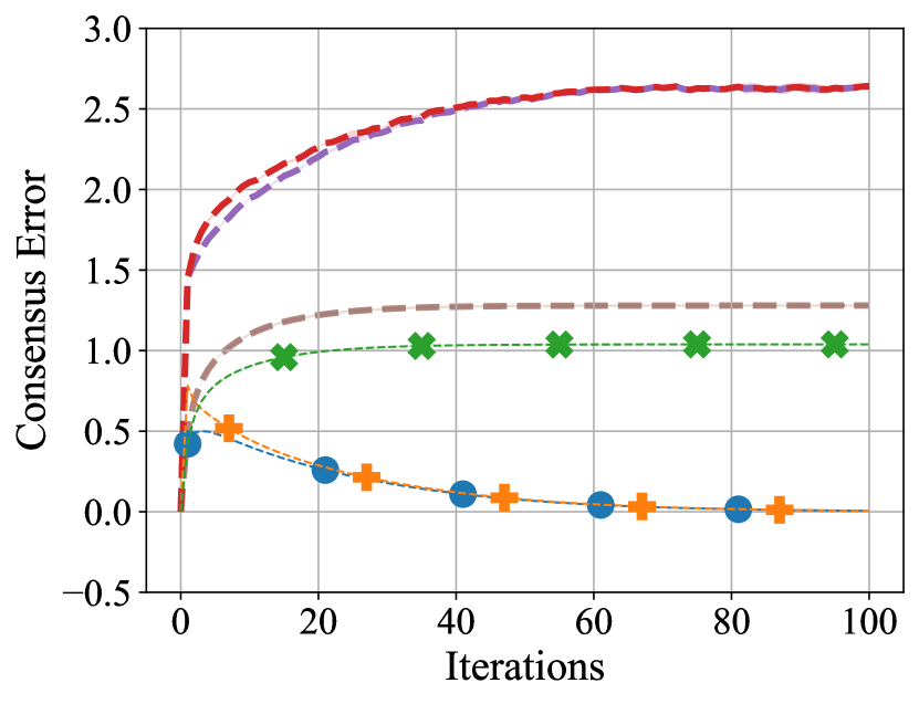
(c) Ring topology

Figure 2: Consensus error vs. iterations with and without noise for different communication topologies. Note the different Y-axis scale in Fig (a) as compared with Fig (b) and (c) for better readability.

IV Experiments

In this section, we perform several experiments on regression problems to verify the impact of noise on the convergence of the three proposed algorithms as established in Theorem 1. We consider the case when the number of clients, $n$ = 16. The experiments are repeated three times, and the results (loss/consensus error) are averaged. We use the mean-squared error loss function with $L_{2}$ regularization. The learning rate of the model is set as 0.2 with a decay of 0.9 with every iteration. We describe the dataset generation next.

Linear Regression Dataset: We generate a synthetic data samples ($m$ = 10000) ${(x_{i};y_{i})}^{m}_{i=1}$ according to $y_{i}=\langle w,x_{i}\rangle+\epsilon_{i}$, where $w\in\mathbb{R}^{2000}$, $x_{i}\sim\mathcal{N}(0;I_{2000})$ and noise, $\epsilon_{i}\sim\mathcal{N}(0,0.05)$.

The experiments are performed with various levels of noise variance, $D_{t,i}^{2}$ for all $t,i$, as described in the algorithms, for various communication topologies, namely the ring, torus, and fully connected network. The mixing matrix can be defined as a weighted adjacency matrix of a given communication graph[38]. The nonzero weights in the mixing matrix for ring topology are equal to $\frac{1}{3}$, in the torus topology $\frac{1}{5}$, and fully connected topology, $\frac{1}{n}$.

We first perform the experiments with no noise as a baseline and then gradually increase the noise variance to study the robustness of the algorithms. For the purpose of consistency, we have shown the results of the experiments with noise variance $D_{t,i}^{2}=0.005$ in Figures 1 and 2 along with no noise scenario. The experiments were performed on Intel Xeon Gold workstation.

IV-A Discussion

We performed numerical experiments on the algorithms with and without noise for different topologies. We observed, see Figure 1, that the algorithms FedNDL1 and FedNDL2 perform poorly in terms of convergence due to noise presence which is consistent with Theorem 1. In addition, as it can be seen in Figure 2, the consensus error also increases with the noise which is also consistent with our theoretical analysis presented in Theorem 1.

On the other hand, the algorithm FedNDL3 is observed to be the most robust as it does not diverge in the presence of added channel noise. The noise term for the FedNDL3 in the upper bound given in Theorem 1 is of order $\mathcal{O}({T^{-\frac{1}{2}}})$, whereas it is of order $\mathcal{O}({T^{\frac{3}{2}}})$ for FedNDL1 and FedNDL2. This effect of the noise can also be observed in  Figure 1.

The consensus error is strongly dependent on the communication network. We can observe that the consensus error is much lower for the fully connected network and significantly higher for the ring topology for the same algorithm in the presence of noise. The consensus error function plots in Figure 2 are consistent with the connectivity of the communication network (number of client interactions). The fully connected topology encompasses the maximum number of clients interaction. It therefore, yields the lowest consensus error, followed by the torus topology and then the ring topology, which has the lowest number of client interactions.

V Conclusion and Future Work

We studied the impact of noisy communication channels on the convergence of DFL. We proposed multiple scenarios for establishing consensus in the presence of noise and provided experimental results on all the algorithms. Additionally, we provided theoretical results for FedNDL1, FedNDL2 and FedNDL3, under the assumption of smooth non-convex function, and we observed that in FeDNDL3, the noise term in the upper bound given by Theorem 1 is of order $\mathcal{O}({T^{-\frac{1}{2}}})$ and is independent of communication topology. In contrast, the impact of noise on the convergence of FedNDL1, FedNDL2 increases with $T$ and weaker communication structures. We conducted numerical experiments on a synthetically generated dataset and observed that FedNDL3 is more robust against the added noise than the other two algorithms analyzed in this paper.

Future research should focus on a formal study of the benefits of multi-round gossiping [3], or acceleration methods such as Chebyshev acceleration [36, 37], and establishing statistical lower bounds on the convergence of the algorithms under the presence of noise in communication channels. The algorithms should also be tested on large-scale deep-learning datasets as well as for different network topologies.

Appendix A Theorems

Theorem 2 (Smooth non-convex case for FedNDL1).

Suppose Assumptions 1, 2, 3, 4 and 5 hold. Let $\eta L<\frac{1}{6}$, $\rho>2\sqrt{6}\eta L$, and $f^{*}=\min_{x\in\mathbb{R}^{d}}f(x)$, for $\phi>\frac{L^{2}\eta(\frac{1}{2}+2L\eta)}{[\frac{\rho}{2}-\frac{12L^{2}\eta^{2}}{\rho}]}$, we have ,

$$\frac{1}{T}\sum_{t=1}^{T}\operatorname{\mathbb{E}}[\|\nabla f(\bar{X}_{t})\|^{2}]+\frac{L^{2}}{2}\frac{1}{T}\sum_{t=1}^{T}\operatorname{\mathbb{E}}[(C.E)_{t}]\\ \leq\frac{2(f(\bar{X}_{1})-f^{*}+\phi(C.E)_{1})}{\eta(1-4\eta L)}+\frac{2\eta(\phi(1-\rho)+\frac{L}{n})}{(1-4\eta L)}\sigma^{2}\\ +\frac{16\phi\eta B^{2}}{(1-4\eta L)\rho}+\frac{2\Big{(}L+\phi\big{[}\frac{\rho}{2}+\frac{2}{\rho}\big{]}\Big{)}}{\eta(1-4\eta L)}\frac{1}{nT}\sum_{t=1}^{T}\sum_{i=1}^{n}{D}^{2}_{t,i}$$ (12)

Theorem 3 (Smooth non-convex case for FedNDL2).

Suppose Assumptions 1, 2, 3, 4 and 5 hold. Let $\eta L<\frac{1}{12}$, $\rho>4\sqrt{3}\eta L$ and $f^{*}=\min_{x\in\mathbb{R}^{d}}f(x)$, for $\phi>\frac{L^{2}\eta(1+2L\eta)(1-\rho)}{[\frac{\rho}{2}-\frac{24L^{2}\eta^{2}}{\rho}]}$, we have

$$\frac{1}{T}\sum_{t=1}^{T}\operatorname{\mathbb{E}}[\|\nabla f(\bar{X}_{t})\|^{2}]+\frac{L^{2}}{T}\sum_{t=1}^{T}\operatorname{\mathbb{E}}[(C.E)_{t}]\\ \leq\frac{2(f(\bar{X}_{1})-f^{*}+\phi(C.E)_{1})}{\eta(1-2\eta L)T}+\frac{2\eta(\phi+\frac{L}{n})}{(1-2\eta L)}\sigma^{2}+\frac{8\phi\eta(1+\frac{2}{\rho})}{(1-2\eta L)}B^{2}\\ +\frac{2\Big{(}L^{2}[\eta(1+2L\eta)+2]+4\phi[1-\rho+\frac{24L^{2}\eta^{2}}{\rho}]\Big{)}}{\eta(1-2\eta L)}\frac{1}{nT}\sum_{t=1}^{T}\sum_{i=1}^{n}D_{t,i}^{2}$$ (13)

Theorem 4 (Smooth non-convex case for FedNDL-3).

Suppose Assumptions 1, 2, 3, 4, 5 and 6 hold. Let $\eta L<\frac{1}{6}$ and $f^{*}=\min_{x\in\mathbb{R}^{d}}f(x)$, for $\phi_{t}=L^{2}\eta(1+2L\eta)+2\phi_{t+1}\rho_{t}$, we have

$$\frac{1}{T}\sum_{t=1}^{T}\operatorname{\mathbb{E}}[\|\nabla f(\bar{X}_{t})\|^{2}]+\frac{2L^{2}}{T}\sum_{t=1}^{T}\operatorname{\mathbb{E}}[(C.E)_{t}]\\ \leq\frac{2(f(\bar{X}_{1})-f^{*}+\phi_{1}(C.E)_{1})}{\eta(1-2L\eta)T}+\frac{L\eta}{n(1-2L\eta)}\sigma^{2}\\ +\frac{L^{2}(1-6L\eta)}{T(1-2L\eta)}\sum_{t=1}^{T}\frac{\gamma_{t}}{\rho_{t}}+\frac{L\eta}{(1-2L\eta)}\frac{1}{nT}\sum_{t=1}^{T}\sum_{i=1}^{n}{D}^{2}_{t,i}$$ (14)

Proof.

We start by defining the notations we use in the theoretical analysis of the algorithm.
Vectors:

$$X_{t}^{i}:\text{Parameter of client $i$ at time $t$}$$ (15)

$$\nabla_{t,i}=\nabla f(X_{t}^{i})\text{ and }\widetilde{\nabla}_{t,i}=\widetilde{\nabla}f(X_{t}^{i},\xi_{t}^{i})$$ (16)

$$\bar{X}_{t}=\frac{1}{n}\sum_{i=1}^{n}X_{t}^{i}$$ (17)

$$\bar{\nabla}_{t}=\nabla f(\bar{X}_{t})$$ (18)

$$\bar{\delta}_{t}=\frac{1}{n}\sum_{i=1}^{n}\delta_{t}^{i}$$ (19)

Matrix form:

$$X^{t}=[X_{t}^{1},X_{t}^{2},\cdots,X_{t}^{n}]\in\mathbb{R}^{d\times n}$$ (20)

$$\bar{X}^{t}=[\bar{X}_{t},\bar{X}_{t},\cdots,\bar{X}_{t}]\in\mathbb{R}^{d\times n}$$ (21)

$$\nabla^{t}=[\nabla_{t,1},\nabla_{t,2},\cdots,\nabla_{t,n}]\in\mathbb{R}^{d\times n}$$ (22)

$$\widetilde{\nabla}^{t}=[\widetilde{\nabla}_{t,1},\widetilde{\nabla}_{t,2},\cdots,\widetilde{\nabla}_{t,n}]\in\mathbb{R}^{d\times n}$$ (23)

$$\bar{\nabla}^{t}=[\bar{\nabla}_{t},\bar{\nabla}_{t},\cdots,\bar{\nabla}_{t}]\in\mathbb{R}^{d\times n}$$ (24)

$$\delta^{t}=[\delta_{t}^{1},\delta_{t}^{2},\cdots,\delta_{t}^{n}]\in\mathbb{R}^{d\times n}$$ (25)

$$\bar{\delta}^{t}=[\bar{\delta}_{t},\bar{\delta}_{t},\cdots,\bar{\delta}_{t}]\in\mathbb{R}^{d\times n}$$ (26)

Appendix B Proof for FedNDL1

$$X_{t+\frac{1}{2}} =X_{t}-\eta\widetilde{\nabla}_{t,i}$$ (27)

$$X_{t+1} =\Big{(}X_{t+\frac{1}{2}}+\delta_{t,i}\Big{)}W$$ (28)

$$\bar{X}_{t+1} =\bar{X_{t}}-\frac{\eta}{n}\sum_{i=1}^{n}\widetilde{\nabla}_{t,i}+\bar{\delta_{t}}$$ (29)

$$\langle a_{1},a_{1}\rangle=\frac{1}{2}(\|a_{1}\|^{2}+\|a_{2}\|^{2}-\|a_{1}-a_{2}\|^{2})$$ (30)

Using the $L-$smoothness assumption we get,

$$f(\bar{X}_{t+1}) \leq f(\bar{X_{t}})+\langle\nabla f(\bar{x}_{t}),\bar{X}_{t+1}-\bar{X_{t}}\rangle+\frac{L}{2}\|\bar{X}_{t+1}-\bar{X}_{t}\|^{2}$$ (31)

$$\leq f(\bar{X_{t}})+\langle\nabla f(\bar{x}_{t}),-\frac{\eta}{n}\sum_{i=1}^{n}\widetilde{\nabla}_{t,i}+\bar{\delta_{t}}\rangle+\frac{L}{2}\|-\frac{\eta}{n}\sum_{i=1}^{n}\widetilde{\nabla}_{t,i}+\bar{\delta_{t}}\|^{2}$$ (32)

Now, taking expectation w.r.t data and alongside the zero mean the assumption of noise in eq. 32 we get

$$\operatorname{\mathbb{E}}[f(\bar{X}_{t+1})]\leq\operatorname{\mathbb{E}}[f(\bar{X_{t}})]+\underbrace{\operatorname{\mathbb{E}}[\langle\nabla f(\bar{x}_{t}),-\frac{\eta}{n}\sum_{i=1}^{n}\widetilde{\nabla}_{t,i}\rangle]}_{Term\ 1}+\underbrace{\frac{L}{2}\operatorname{\mathbb{E}}[\|-\frac{\eta}{n}\sum_{i=1}^{n}\widetilde{\nabla}_{t,i}+\bar{\delta_{t}}\|^{2}]}_{Term\ 2}$$ (33)

Starting with $Term\ 1:$

$$\operatorname{\mathbb{E}}[\langle\nabla f(\bar{x}_{t}),-\frac{\eta}{n}\sum_{i=1}^{n}\widetilde{\nabla}_{t,i}\rangle] =-\eta\operatorname{\mathbb{E}}[\langle\bar{\nabla}_{t},\frac{1}{n}\sum_{i=1}^{n}\widetilde{\nabla}_{t,i}\rangle]$$ (34)

$$=-\eta\operatorname{\mathbb{E}}[\langle\bar{\nabla}_{t},\frac{1}{n}\sum_{i=1}^{n}(\widetilde{\nabla}_{t,i}+\nabla_{t,i}-\nabla_{t,i})\rangle]$$ (35)

$$=-\eta\operatorname{\mathbb{E}}[\langle\bar{\nabla}_{t},\frac{1}{n}\sum_{i=1}^{n}\nabla_{t,i}\rangle]-\eta\operatorname{\mathbb{E}}[\langle\bar{\nabla}_{t},\frac{1}{n}\sum_{i=1}^{n}(\widetilde{\nabla}_{t,i}-\nabla_{t,i})\rangle]$$ (36)

The second term in eq. 36 will be zero, since $\operatorname{\mathbb{E}}[\widetilde{\nabla}_{t,i}]=\operatorname{\mathbb{E}}[\nabla_{t,i}].$ Now focusing on first term in eq. 36 and using eq. 30, we have

$$\operatorname{\mathbb{E}}[\langle\nabla f(\bar{x}_{t}),-\frac{\eta}{n}\sum_{i=1}^{n}\widetilde{\nabla}_{t,i}\rangle] =-\eta\operatorname{\mathbb{E}}[\langle\bar{\nabla}_{t},\frac{1}{n}\sum_{i=1}^{n}\nabla_{t,i}\rangle]$$ (37)

$$=-\frac{\eta}{2}\operatorname{\mathbb{E}}\Big{[}\|\bar{\nabla}_{t}\|^{2}+\|\frac{1}{n}\sum_{i=1}^{n}\nabla_{t,i}\|^{2}-\|\bar{\nabla}_{t}-\frac{1}{n}\sum_{i=1}^{n}\nabla_{t,i}\|^{2}\Big{]}$$ (38)

Now, using $Term\ 2:$

$$\frac{L}{2}\operatorname{\mathbb{E}}[\|\bar{\delta_{t}}-\frac{\eta}{n}\sum_{i=1}^{n}\widetilde{\nabla}_{t,i}\|^{2}] =\frac{L}{2}(\operatorname{\mathbb{E}}[\|\bar{\delta_{t}}\|^{2}]+\operatorname{\mathbb{E}}[\|\frac{\eta}{n}\sum_{i=1}^{n}\widetilde{\nabla}_{t,i}\|^{2}]-\operatorname{\mathbb{E}}[\langle\bar{\delta_{t}},\frac{\eta}{n}\sum_{i=1}^{n}\widetilde{\nabla}_{t,i}\rangle])$$ (39)

Using Young’s inequality above, we have

$$\frac{L}{2}\operatorname{\mathbb{E}}[\|\bar{\delta_{t}}-\frac{\eta}{n}\sum_{i=1}^{n}\widetilde{\nabla}_{t,i}\|^{2}] =L\Big{(}\underbrace{\operatorname{\mathbb{E}}[\|\bar{\delta_{t}}\|^{2}]}_{P}+\underbrace{\eta^{2}\operatorname{\mathbb{E}}[\|\frac{1}{n}\sum_{i=1}^{n}\widetilde{\nabla}_{t,i}\|^{2}]}_{Q}\Big{)}$$ (40)

Solving $P:$

$$\operatorname{\mathbb{E}}[\|\bar{\delta_{t}}\|^{2}] =\operatorname{\mathbb{E}}[\|\frac{1}{n}\sum_{i=1}^{n}\delta_{t,i}\|^{2}]$$ (41)

$$\leq\frac{1}{n}\sum_{i=1}^{n}\operatorname{\mathbb{E}}[\|\delta_{t,i}\|^{2}]$$ (42)

$$\leq\frac{1}{n}\sum_{i=1}^{n}{D}^{2}_{t,i}$$ (43)

Here, eq. 42 follows due to Jensen’s Inequality and eq. 43 follows due to Assumption 6. Solving $Q:$

$$\eta^{2}\operatorname{\mathbb{E}}[\|\frac{1}{n}\sum_{i=1}^{n}\widetilde{\nabla}_{t,i}\|^{2}] =\eta^{2}\operatorname{\mathbb{E}}[\|\frac{1}{n}\sum_{i=1}^{n}(\widetilde{\nabla}_{t,i}+\nabla_{t,i}-\nabla_{t,i})\|^{2}]$$ (44)

$$\leq\eta^{2}\Big{[}\frac{\sigma^{2}}{n}+\operatorname{\mathbb{E}}[\|\frac{1}{n}\sum_{i=1}^{n}\nabla_{t,i}\|^{2}]\Big{]}$$ (45)

Now, combining the results from eq. 38, eq. 43, eq. 45, and putting it back in eq. 33, we get

$$\operatorname{\mathbb{E}}[f(\bar{X}_{t+1})]\leq\operatorname{\mathbb{E}}[f(\bar{X_{t}})]-\frac{\eta}{2}\operatorname{\mathbb{E}}[\|\bar{\nabla}_{t}\|^{2}]-\underbrace{\frac{\eta}{2}\operatorname{\mathbb{E}}[\|\frac{1}{n}\sum_{i=1}^{n}\nabla_{t,i}\|^{2}]}_{M}+\frac{\eta}{2}\operatorname{\mathbb{E}}[\|\bar{\nabla}_{t}-\frac{1}{n}\sum_{i=1}^{n}\nabla_{t,i}\|^{2}]+\frac{L}{n}\sum_{i=1}^{n}{D}^{2}_{t,i}$$

$$+\frac{L\eta^{2}}{n}\sigma^{2}+\underbrace{L\eta^{2}\operatorname{\mathbb{E}}[\|\frac{1}{n}\sum_{i=1}^{n}\nabla_{t,i}\|^{2}]}_{N}$$ (46)

In the equation above reducing $N$ as follows,

$$N =L\eta^{2}\operatorname{\mathbb{E}}[\|\frac{1}{n}\sum_{i=1}^{n}\nabla_{t,i}\|^{2}]$$ (47)

$$=L\eta^{2}\operatorname{\mathbb{E}}[\|\frac{1}{n}\sum_{i=1}^{n}\nabla_{t,i}-\bar{\nabla_{t}}+\bar{\nabla_{t}}\|^{2}]$$ (48)

$$\leq 2L\eta^{2}\operatorname{\mathbb{E}}[\|\bar{\nabla_{t}}\|^{2}]+2L\eta^{2}\operatorname{\mathbb{E}}[\|\frac{1}{n}\sum_{i=1}^{n}\nabla_{t,i}-\bar{\nabla_{t}}\|^{2}]$$ (49)

Here, eq. 49 follows due to Young’s Inequality. So, dropping $M$ and putting eq. 49 back in eq. 46, we have

$$\operatorname{\mathbb{E}}[f(\bar{X}_{t+1})]\leq\operatorname{\mathbb{E}}[f(\bar{X_{t}})]-\eta(\frac{1}{2}-2L\eta)\operatorname{\mathbb{E}}[\|\bar{\nabla}_{t}\|^{2}]+\frac{L}{n}\sum_{i=1}^{n}{D}^{2}_{t,i}+\frac{L\eta^{2}}{n}\sigma^{2}$$

$$+(\frac{\eta}{2}+2L\eta^{2})\operatorname{\mathbb{E}}[\|\frac{1}{n}\sum_{i=1}^{n}\nabla_{t,i}-\bar{\nabla_{t}}\|^{2}]$$ (50)

$$\eta(\frac{1}{2}-2L\eta)\operatorname{\mathbb{E}}[\|\bar{\nabla}_{t}\|^{2}]\leq(\operatorname{\mathbb{E}}[f(\bar{X_{t}})]-\operatorname{\mathbb{E}}[f(\bar{X}_{t+1})])+\frac{L}{n}\sum_{i=1}^{n}{D}^{2}_{t,i}+\frac{L\eta^{2}}{n}\sigma^{2}$$

$$+(\frac{\eta}{2}+2L\eta^{2})\underbrace{\operatorname{\mathbb{E}}[\|\frac{1}{n}\sum_{i=1}^{n}\nabla_{t,i}-\bar{\nabla_{t}}\|^{2}]}_{C}$$ (51)

We need to study C:

$$C =\operatorname{\mathbb{E}}[\|\frac{1}{n}\sum_{i=1}^{n}\nabla_{t,i}-\bar{\nabla_{t}}\|^{2}]$$ (52)

$$\leq L^{2}\underbrace{\frac{1}{n}\sum_{i=1}^{n}\operatorname{\mathbb{E}}[\|X_{t,i}-\bar{X}_{t}\|^{2}]}_{Consensus\ Error}$$ (53)

Now, let us study the consensus error at $t+1$. So, we reformulate the consensus error by using the Frobenius norm, we start with,

$$\frac{1}{n}\operatorname{\mathbb{E}}\Big{[}\Big{\|}\bar{X}^{t+1}-{X}^{t+1}\Big{\|}^{2}_{F}\Big{]} =\frac{1}{n}\operatorname{\mathbb{E}}\Big{[}\Big{\|}\Big{[}\bar{X}^{t}-\eta\widetilde{\nabla}^{t}\frac{\mathds{1}\mathds{1}^{\top}}{n}+\bar{\delta}^{t}-{X}^{t}+\eta\widetilde{\nabla}^{t}-\delta^{t}\Big{]}W\Big{\|}^{2}_{F}\Big{]}$$ (54)

$$=\frac{1}{n}\operatorname{\mathbb{E}}\Big{[}\Big{\|}\Big{[}\bar{X}^{t}-{X}^{t}-\eta(\widetilde{\nabla}^{t}\frac{\mathds{1}\mathds{1}^{\top}}{n}-\widetilde{\nabla}^{t})+(\bar{\delta}^{t}-\delta^{t})\Big{]}W\Big{\|}^{2}_{F}\Big{]}$$ (55)

$$\leq\frac{(1-\rho)}{n}\operatorname{\mathbb{E}}\Big{[}\Big{\|}\Big{[}\bar{X}^{t}-{X}^{t}-\eta(\widetilde{\nabla}^{t}\frac{\mathds{1}\mathds{1}^{\top}}{n}-\widetilde{\nabla}^{t})+(\bar{\delta}^{t}-\delta^{t})+\eta(\nabla^{t}\frac{\mathds{1}\mathds{1}^{\top}}{n}-\nabla^{t})$$

$$-\eta(\nabla^{t}\frac{\mathds{1}\mathds{1}^{\top}}{n}-\nabla^{t})\Big{]}\Big{\|}^{2}_{F}\Big{]}$$ (56)

Let, $a=(\bar{X}^{t}-{X}^{t}-\eta(\nabla^{t}\frac{\mathds{1}\mathds{1}^{\top}}{n}-\nabla^{t}))$, $b=\eta((\nabla^{t}\frac{\mathds{1}\mathds{1}^{\top}}{n}-\nabla^{t})-(\widetilde{\nabla}^{t}\frac{\mathds{1}\mathds{1}^{\top}}{n}-\widetilde{\nabla}^{t}))$, and $c=(\bar{\delta}^{t}-\delta^{t})$. Using this in eq. 56, we have

$$\frac{1}{n}\operatorname{\mathbb{E}}\Big{[}\Big{\|}\bar{X}^{t+1}-{X}^{t+1}\Big{\|}^{2}_{F}\Big{]}\leq\frac{(1-\rho)}{n}\operatorname{\mathbb{E}}\Big{[}\big{\|}a\big{\|}^{2}_{F}+\big{\|}b\big{\|}^{2}_{F}+\big{\|}c\big{\|}^{2}_{F}+2\langle a,b\rangle+2\langle b,c\rangle+2\langle c,a\rangle\Big{]}$$ (57)

In the result above, $\operatorname{\mathbb{E}}[\langle a,b\rangle]=0$, $\operatorname{\mathbb{E}}[\langle b,c\rangle]=0$, and $\operatorname{\mathbb{E}}[\langle c,a\rangle]=0$.

$$\frac{1}{n}\operatorname{\mathbb{E}}\Big{[}\Big{\|}\bar{X}^{t+1}-{X}^{t+1}\Big{\|}^{2}_{F}\Big{]} \leq\frac{(1-\rho)}{n}\operatorname{\mathbb{E}}\Big{[}\big{\|}a\big{\|}^{2}_{F}+\big{\|}b\big{\|}^{2}_{F}+\big{\|}c\big{\|}^{2}_{F}\Big{]}$$

$$\frac{1}{n}\operatorname{\mathbb{E}}\Big{[}\Big{\|}\bar{X}^{t+1}-{X}^{t+1}\Big{\|}^{2}_{F}\Big{]} \leq\underbrace{\frac{(1-\rho)}{n}\operatorname{\mathbb{E}}\Big{[}\big{\|}a\big{\|}^{2}_{F}\Big{]}}_{J}+\underbrace{\frac{(1-\rho)}{n}\operatorname{\mathbb{E}}\Big{[}\big{\|}b\big{\|}^{2}_{F}\Big{]}}_{K}+\underbrace{\frac{(1-\rho)}{n}\operatorname{\mathbb{E}}\Big{[}\big{\|}c\big{\|}^{2}_{F}\Big{]}}_{L}$$ (58)

Solving for Term $J:$

$$\frac{(1-\rho)}{n}\operatorname{\mathbb{E}}\Big{[}\big{\|}a\big{\|}^{2}_{F}\Big{]} =\frac{(1-\rho)}{n}\operatorname{\mathbb{E}}\Big{[}\big{\|}\bar{X}^{t}-{X}^{t}-\eta(\nabla^{t}\frac{\mathds{1}\mathds{1}^{\top}}{n}-\nabla^{t})\big{\|}^{2}_{F}\Big{]}$$

$$=\frac{(1-\rho)(1+\frac{\rho}{2})}{n}\operatorname{\mathbb{E}}\Big{[}\big{\|}\bar{X}^{t}-{X}^{t}\big{\|}^{2}_{F}\Big{]}+\frac{\eta^{2}(1-\rho)(1+\frac{2}{\rho})}{n}\underbrace{\operatorname{\mathbb{E}}\Big{[}\big{\|}(\nabla^{t}\frac{\mathds{1}\mathds{1}^{\top}}{n}-\nabla^{t})\big{\|}^{2}_{F}\Big{]}}_{J_{1}}$$ (59)

Solving for Term $J_{1}:$

$$J_{1} =\sum_{i=1}^{n}\operatorname{\mathbb{E}}\Big{[}\big{\|}\frac{1}{n}\sum_{j=1}^{n}\nabla f_{j}(x_{t}^{j})-\nabla f_{i}(x_{t}^{i})+\nabla f(\bar{X}_{t})-\nabla f(\bar{X}_{t})\big{\|}^{2}\Big{]}$$

$$\leq 2\sum_{i=1}^{n}\operatorname{\mathbb{E}}\Big{[}\big{\|}\frac{1}{n}\sum_{j=1}^{n}(\nabla f_{j}(x_{t}^{j})-f_{j}(\bar{X}_{t}))\big{\|}^{2}\Big{]}+2\sum_{i=1}^{n}\operatorname{\mathbb{E}}\Big{[}\big{\|}\nabla f_{i}(x_{t}^{i})-\nabla f(\bar{X}_{t})\big{\|}^{2}\Big{]}$$ (60)

$$\leq 2\sum_{j=1}^{n}\operatorname{\mathbb{E}}\Big{[}\big{\|}\nabla f_{j}(x_{t}^{j})-f_{j}(\bar{X}_{t})\big{\|}^{2}\Big{]}+2\sum_{i=1}^{n}\operatorname{\mathbb{E}}\Big{[}\big{\|}\nabla f_{i}(x_{t}^{i})-\nabla f(\bar{X}_{t})+\nabla f(x_{t}^{i})-\nabla f(x_{t}^{i})\big{\|}^{2}\Big{]}$$ (61)

$$\leq 2L^{2}\operatorname{\mathbb{E}}\Big{[}\big{\|}\bar{X}_{t}-X^{t}\big{\|}^{2}_{F}\Big{]}+4\sum_{i=1}^{n}\operatorname{\mathbb{E}}\Big{[}\big{\|}\nabla f_{i}(x_{t}^{i})-\nabla f(x_{t}^{i})\big{\|}^{2}\Big{]}+4\sum_{i=1}^{n}\operatorname{\mathbb{E}}\Big{[}\big{\|}\nabla f(\bar{X}_{t})-\nabla f(x_{t}^{i})\big{\|}^{2}\Big{]}$$ (62)

$$\leq 6L^{2}\operatorname{\mathbb{E}}\Big{[}\big{\|}\bar{X}_{t}-X^{t}\big{\|}^{2}_{F}\Big{]}+4nB^{2}$$ (63)

In eq. 60 follows due to Young’s inequality and eq. 61 follows due to Jensen’s inequality. Again, eq. 62 follows due to Young’s inequality and the Frobenius norm. Similarly, eq. 63 holds due to $L-$smoothness and assumption 5. So, putting the result obtained for $J_{1}$ in eq. 59, Term $J$ becomes,

$$J\leq\frac{(1-\rho)(1+\frac{\rho}{2})}{n}\operatorname{\mathbb{E}}\Big{[}\big{\|}\bar{X}^{t}-{X}^{t}\big{\|}^{2}_{F}\Big{]}+\frac{\eta^{2}(1-\rho)(1+\frac{2}{\rho})}{n}\Big{(}6L^{2}\operatorname{\mathbb{E}}\Big{[}\big{\|}\bar{X}_{t}-X^{t}\big{\|}^{2}_{F}\Big{]}+4nB^{2}\Big{)}$$ (64)

Now, using the fact that $\frac{(1-\rho)(1+\frac{\rho}{2})}{n}\leq\frac{(1-\frac{\rho}{2})}{n}$ and $\frac{\eta^{2}(1-\rho)(1+\frac{2}{\rho})}{n}\leq\frac{2\eta^{2}}{n\rho}$ in the equation above, we get

$$J\leq\frac{1}{n}\Big{[}(1-\frac{\rho}{2})+\frac{12L^{2}\eta^{2}}{\rho}\Big{]}\operatorname{\mathbb{E}}\Big{[}\big{\|}\bar{X}^{t}-{X}^{t}\big{\|}^{2}_{F}\Big{]}+\frac{8\eta^{2}B^{2}}{\rho}$$ (65)

Now, solving Term $K:$

$$K =\frac{(1-\rho)}{n}\operatorname{\mathbb{E}}\Big{[}\big{\|}\eta\Big{(}(\nabla^{t}\frac{\mathds{1}\mathds{1}^{\top}}{n}-\nabla^{t})-(\widetilde{\nabla}^{t}\frac{\mathds{1}\mathds{1}^{\top}}{n}-\widetilde{\nabla}^{t})\Big{)}\big{\|}^{2}_{F}\Big{]}$$ (66)

$$K \leq(1-\rho)\eta^{2}\sigma^{2}$$ (67)

In eq. 67 follows due to Assumption 3. Now, solving Term $L:$

$$L =\frac{(1-\rho)}{n}\operatorname{\mathbb{E}}\big{[}\big{\|}\bar{\delta}^{t}-\delta^{t}\big{\|}^{2}_{F}\big{]}$$ (68)

$$\leq\frac{(1-\rho)(1+\frac{\rho}{2})}{n}\operatorname{\mathbb{E}}\big{[}\big{\|}\bar{\delta}^{t}\|^{2}_{F}\big{]}+\frac{(1-\rho)(1+\frac{2}{\rho})}{n}\operatorname{\mathbb{E}}\big{[}\big{\|}\delta^{t}\big{\|}^{2}_{F}\big{]}$$ (69)

$$\leq\frac{(1-\rho)(1+\frac{\rho}{2})}{n}\sum_{j=1}^{n}\operatorname{\mathbb{E}}\big{[}\big{\|}\bar{\delta}^{t}\|^{2}\big{]}+\frac{(1-\rho)(1+\frac{2}{\rho})}{n}\sum_{j=1}^{n}\operatorname{\mathbb{E}}\big{[}\big{\|}\delta_{t}^{j}\big{\|}^{2}\big{]}$$ (70)

$$\leq\frac{(1-\rho)(1+\frac{\rho}{2})}{n}n\operatorname{\mathbb{E}}\big{[}\big{\|}\frac{1}{n}\sum_{i=1}^{n}\delta_{t}^{i}\|^{2}\big{]}+\frac{(1-\rho)(1+\frac{2}{\rho})}{n}\sum_{i=1}^{n}{D}^{2}_{t,i}$$ (71)

$$\leq\frac{(1-\rho)(1+\frac{\rho}{2})}{n}\sum_{i=1}^{n}\operatorname{\mathbb{E}}\big{[}\big{\|}\delta_{t}^{i}\big{\|}^{2}\big{]}+\frac{(1-\rho)(1+\frac{2}{\rho})}{n}\sum_{i=1}^{n}{D}^{2}_{t,i}$$ (72)

$$\leq\frac{(1-\rho)(1+\frac{\rho}{2})}{n}\sum_{i=1}^{n}{D}^{2}_{t,i}+\frac{(1-\rho)(1+\frac{2}{\rho})}{n}\sum_{i=1}^{n}{D}^{2}_{t,i}$$ (73)

$$\leq\frac{1}{n}(1-\rho)\Big{[}2+\frac{\rho}{2}+\frac{2}{\rho}\Big{]}\sum_{i=1}^{n}{D}^{2}_{t,i}$$ (74)

$$\leq\frac{1}{n}\Big{[}\frac{\rho}{2}+\frac{2}{\rho}\Big{]}\sum_{i=1}^{n}{D}^{2}_{t,i}$$ (75)

So, using the results for $J$, $K$, and $L$ in eq. 58, we get

$$\frac{1}{n}\operatorname{\mathbb{E}}\Big{[}\Big{\|}\bar{X}^{t+1}-{X}^{t+1}\Big{\|}^{2}_{F}\Big{]} \leq J+K+L$$

$$\leq\frac{1}{n}\Big{[}(1-\frac{\rho}{2})+\frac{12L^{2}\eta^{2}}{\rho}\Big{]}\operatorname{\mathbb{E}}\Big{[}\big{\|}\bar{X}^{t}-{X}^{t}\big{\|}^{2}_{F}\Big{]}+\frac{8\eta^{2}B^{2}}{\rho}+(1-\rho)\eta^{2}\sigma^{2}$$

$$+\frac{1}{n}\Big{[}\frac{\rho}{2}+\frac{2}{\rho}\Big{]}\sum_{i=1}^{n}{D}^{2}_{t,i}$$ (76)

From here on we are going to use the shorthand, $(C.E)_{t}$ for $\frac{1}{n}\Big{\|}\bar{X}^{t}-{X}^{t}\Big{\|}^{2}_{F}$. So, using the shorthand in eq. 76, we have

$$\operatorname{\mathbb{E}}[(C.E)_{t+1}]\leq\Big{[}(1-\frac{\rho}{2})+\frac{12L^{2}\eta^{2}}{\rho}\Big{]}\operatorname{\mathbb{E}}[(C.E)_{t}]+\frac{8\eta^{2}B^{2}}{\rho}+(1-\rho)\eta^{2}\sigma^{2}+\frac{1}{n}\Big{[}\frac{\rho}{2}+\frac{2}{\rho}\Big{]}\sum_{i=1}^{n}{D}^{2}_{t,i}$$ (77)

Let there be a potential function $\psi_{t}$, defined as,

$$\psi_{t}=f(\bar{X}_{t})+\phi\operatorname{\mathbb{E}}[(C.E)_{t}],{\text{ where $\phi$ is a constant.}}$$ (78)

Now, we use the potential function to complete the proof.

$$\psi_{t+1}-\psi_{t}=\big{\{}f(\bar{X}_{t+1})-f(\bar{X}_{t})\big{\}}+\phi\big{\{}\operatorname{\mathbb{E}}[(C.E)_{t+1}]-\operatorname{\mathbb{E}}[(C.E)_{t}]\big{\}}$$ (79)

$$\psi_{t+1}-\psi_{t}\leq-\frac{\eta}{2}(1-4\eta L)\operatorname{\mathbb{E}}[\|\bar{\nabla}_{t}\|^{2}]+\frac{L}{n}\sum_{i=1}^{n}{D}^{2}_{t,i}+\frac{L\eta^{2}}{n}\sigma^{2}+\phi\frac{8\eta^{2}B^{2}}{\rho}+\phi(1-\rho)\eta^{2}\sigma^{2}$$

$$+\Big{[}L^{2}\eta(\frac{1}{2}+2L\eta)-\phi\Big{(}\frac{\rho}{2}-\frac{12L^{2}\eta^{2}}{\rho}\Big{)}\Big{]}\operatorname{\mathbb{E}}[(C.E)_{t}]+\frac{\phi}{n}\Big{[}\frac{\rho}{2}+\frac{2}{\rho}\Big{]}\sum_{i=1}^{n}{D}^{2}_{t,i}$$ (80)

For $\phi>\frac{L^{2}\eta(\frac{1}{2}+2L\eta)}{\frac{\rho}{2}-\frac{12L^{2}\eta^{2}}{\rho}}$ and $\eta L<\frac{\rho}{2\sqrt{6}}$:

$$\operatorname{\mathbb{E}}[\|\bar{\nabla}_{t}\|^{2}]+\frac{2\Big{[}\Big{(}\phi(\frac{\rho}{2}-\frac{12L^{2}\eta^{2}}{\rho})-L^{2}\eta(\frac{1}{2}+2L\eta)\Big{)}\Big{]}}{\eta(1-4\eta L)}\operatorname{\mathbb{E}}[(C.E)_{t}]\leq\frac{2(\psi_{t}-\psi_{t+1})}{\eta(1-4\eta L)}$$

$$+\frac{\eta(\phi(1-\rho)+\frac{L}{n})}{(1-4\eta L)}\sigma^{2}+\frac{16\phi\eta B^{2}}{\rho(1-4\eta L)}+\frac{2\Big{(}L+\phi\Big{[}\frac{\rho}{2}+\frac{2}{\rho}\Big{]}\Big{)}}{\eta(1-4\eta L)}\frac{1}{n}\sum_{i=1}^{n}{D}^{2}_{t,i}$$ (81)

Now let us assume that $\frac{2\Big{[}\Big{(}\phi(\frac{\rho}{2}-\frac{12L^{2}\eta^{2}}{\rho})-L^{2}\eta(\frac{1}{2}+2L\eta)\Big{)}\Big{]}}{\eta(1-4\eta L)}=C$ and we solve for $\phi$:

$$\phi=\frac{C\eta(1-4\eta L)+L^{2}\eta(\frac{1}{2}+4L\eta)}{\frac{\rho}{2}-\frac{12L^{2}\eta^{2}}{\rho}}$$ (82)

So, for $C=L^{2}$, we get $\phi=\frac{2\rho L^{2}\eta}{\rho^{2}-24\eta^{2}L^{2}}$.

Now, summing eq. 81 for $t=\{1\cdots T\}$ and dividing it by $T$, we get

$$\frac{1}{T}\sum_{t=1}^{T}\operatorname{\mathbb{E}}[\|\bar{\nabla}_{t}\|^{2}]+\frac{2\Big{[}\Big{(}\phi(\frac{\rho}{2}-\frac{12L^{2}\eta^{2}}{\rho})-L^{2}\eta(\frac{1}{2}+2L\eta)\Big{)}\Big{]}}{\eta(1-4\eta L)}\frac{1}{T}\sum_{t=1}^{T}\operatorname{\mathbb{E}}[(C.E)_{t}]\leq\frac{2\frac{1}{T}\sum_{t=1}^{T}(\psi_{t}-\psi_{t+1})}{\eta(1-4\eta L)}$$

$$+\frac{\eta(\phi(1-\rho)+\frac{L}{n})}{(1-4\eta L)}\sigma^{2}+\frac{16\phi\eta B^{2}}{\rho(1-4\eta L)}+\frac{2\Big{(}L+\phi\Big{[}\frac{\rho}{2}+\frac{2}{\rho}\Big{]}\Big{)}}{\eta(1-4\eta L)}\frac{1}{nT}\sum_{t=1}^{T}\sum_{i=1}^{n}{D}^{2}_{t,i}$$ (83)

Also, telescoping over eq. 79 and dividing it by $T$, we can write

$$\frac{\psi_{T+1}-\psi_{1}}{T}\geq\frac{f^{*}-f(\bar{X}_{1})-\phi(C.E)_{1}}{T}$$ (84)

We use eq. 84 in eq. 83, we get

$$\frac{1}{T}\sum_{t=1}^{T}\operatorname{\mathbb{E}}[\|\nabla f(\bar{X}_{t})\|^{2}]+\frac{L^{2}}{2}\frac{1}{T}\sum_{t=1}^{T}\operatorname{\mathbb{E}}[(C.E)_{t}]\\ \leq\frac{2(f(\bar{X}_{1})-f^{*}+\phi(C.E)_{1})}{\eta(1-4\eta L)}+\frac{2\eta(\phi(1-\rho)+\frac{L}{n})}{(1-4\eta L)}\sigma^{2}\\ +\frac{16\phi\eta B^{2}}{(1-4\eta L)\rho}+\frac{2\Big{(}L+\phi\big{[}\frac{\rho}{2}+\frac{2}{\rho}\big{]}\Big{)}}{\eta(1-4\eta L)}\frac{1}{nT}\sum_{t=1}^{T}\sum_{i=1}^{n}{D}^{2}_{t,i}$$ (85)

∎

Appendix C Proof for FedNDL2

Start:

$$\bar{X}_{t+1}=\bar{X}_{t}+\bar{\delta}_{t}-\frac{\eta}{n}\sum_{i=1}^{n}\widetilde{\nabla}f_{i}(x_{t+\frac{1}{2}}^{(i)})$$ (86)

Now, using L-smoothness, we get

$$f(\bar{X}_{t+1})\leq f(\bar{X}_{t})+\underbrace{\langle\nabla f(\bar{X}_{t}),\bar{X}_{t+1}-\bar{X}_{t}\rangle}_{Term(A)}+\underbrace{\frac{L}{2}\|\bar{X}_{t+1}-\bar{X}_{t}\|^{2}}_{Term(B)}$$ (87)

Term (A):

$$\langle\nabla f(\bar{X}_{t}),\bar{X}_{t+1}-\bar{X}_{t}\rangle =\langle\nabla f(\bar{X}_{t}),\bar{\delta}_{t}-\frac{\eta}{n}\sum_{i=1}^{n}\widetilde{\nabla}f_{i}(x_{t+\frac{1}{2}}^{(i)})\rangle$$ (88)

$$=\underbrace{\langle\nabla f(\bar{X}_{t}),\bar{\delta}_{t}\rangle}_{Term(A_{1})}+\underbrace{\langle\nabla f(\bar{X}_{t}),-\frac{\eta}{n}\sum_{i=1}^{n}\widetilde{\nabla}f_{i}(x_{t+\frac{1}{2}}^{(i)})\rangle}_{Term(A_{2})}$$ (89)

Term $A_{1}$:

$$\operatorname{\mathbb{E}}[A_{1}] =\operatorname{\mathbb{E}}[\langle\nabla f(\bar{X}_{t}),\bar{\delta}_{t}\rangle]$$ (90)

$$=0$$ (91)

Here eq. 90 follows due to the zero mean of the noise. In term $A_{2}:$ taking the expectation w.r.t to data, we get

$$\operatorname{\mathbb{E}}[\langle\nabla f(\bar{X}_{t}),-\frac{\eta}{n}\sum_{i=1}^{n}\widetilde{\nabla}f_{i}(x_{t+\frac{1}{2}}^{(i)})\rangle]=-\eta\operatorname{\mathbb{E}}[\langle\nabla f(\bar{X}_{t}),\frac{1}{n}\sum_{i=1}^{n}\nabla f_{i}(x_{t+\frac{1}{2}}^{(i)})\rangle]$$ (92)

Using the formulation, $\langle a_{1},a_{2}\rangle=\frac{1}{2}\Big{(}\|a_{1}\|^{2}+\|a_{2}\|^{2}+\|a_{1}-a_{2}\|^{2}\Big{)}$

$$\operatorname{\mathbb{E}}[A_{2}]=-\frac{\eta}{2}\operatorname{\mathbb{E}}[\|\bar{\nabla}_{t}\|^{2}]\underbrace{-\frac{\eta}{2}\operatorname{\mathbb{E}}[\|\frac{1}{n}\sum_{i=1}^{n}\nabla f_{i}(x_{t+\frac{1}{2}}^{(i)})\|^{2}]}_{Term(A_{3})}+\frac{\eta}{2}\operatorname{\mathbb{E}}[\|\bar{\nabla}_{t}-\frac{1}{n}\sum_{i=1}^{n}\nabla f_{i}(x_{t+\frac{1}{2}}^{(i)})\|^{2}]$$ (93)

Putting in the values of $A_{1}$ and $A_{2}$ back in term A we get,

$$\operatorname{\mathbb{E}}[A]\leq-\frac{\eta}{2}\operatorname{\mathbb{E}}[\|\bar{\nabla}_{t}\|^{2}]-\frac{\eta}{2}\operatorname{\mathbb{E}}[\|\frac{1}{n}\sum_{i=1}^{n}\nabla f_{i}(x_{t+\frac{1}{2}}^{(i)})\|^{2}]+\frac{\eta}{2}\operatorname{\mathbb{E}}[\|\bar{\nabla}_{t}-\frac{1}{n}f_{i}(x_{t+\frac{1}{2}}^{i})\|^{2}]$$ (94)

Starting with Term B:

$$\frac{L}{2}\|\bar{X}_{t+1}-\bar{X}_{t}\|^{2} =\frac{L}{2}\|\bar{\delta}_{t}-\frac{\eta}{n}\sum_{i=1}^{n}\widetilde{\nabla}f_{i}(x_{t+\frac{1}{2}}^{(i)})\|^{2}$$ (95)

$$\leq L[\|\bar{\delta}_{t}\|^{2}+\eta^{2}\|\frac{1}{n}\sum_{i=1}^{n}\widetilde{\nabla}f_{i}(x_{t+\frac{1}{2}}^{(i)})\|^{2}]$$ (96)

$$\operatorname{\mathbb{E}}[B] \leq L\operatorname{\mathbb{E}}[\|\bar{\delta}_{t}\|^{2}]+L\eta^{2}\operatorname{\mathbb{E}}[\|\frac{1}{n}\sum_{i=1}^{n}\widetilde{\nabla}f_{i}(x_{t+\frac{1}{2}}^{(i)})\|^{2}]$$ (97)

$$\leq\frac{L}{n}\sum_{i=1}^{n}D_{t,i}^{2}+L\eta^{2}\operatorname{\mathbb{E}}[\|\frac{1}{n}\sum_{i=1}^{n}\big{(}\widetilde{\nabla}f_{i}(x_{t+\frac{1}{2}}^{(i)})-\nabla f_{i}(x_{t+\frac{1}{2}}^{(i)})+\nabla f_{i}(x_{t+\frac{1}{2}}^{(i)})\big{)}\|^{2}]$$ (98)

$$\leq\frac{L}{n}\sum_{i=1}^{n}D_{t,i}^{2}+L\eta^{2}\Big{(}\operatorname{\mathbb{E}}[\|\frac{1}{n}\sum_{i=1}^{n}\big{(}\widetilde{\nabla}f_{i}(x_{t+\frac{1}{2}}^{(i)})-\nabla f_{i}(x_{t+\frac{1}{2}}^{(i)})\big{)}\|^{2}]+\operatorname{\mathbb{E}}[\|\frac{1}{n}\sum_{i=1}^{n}\nabla f_{i}(x_{t+\frac{1}{2}}^{(i)}))\|^{2}\Big{)}]$$

$$+2\operatorname{\mathbb{E}}[\langle\frac{1}{n}\sum_{i=1}^{n}\big{(}\widetilde{\nabla}f_{i}(x_{t+\frac{1}{2}}^{(i)})-\nabla f_{i}(x_{t+\frac{1}{2}}^{(i)})\big{)},\frac{1}{n}\sum_{i=1}^{n}\nabla f_{i}(x_{t+\frac{1}{2}}^{(i)})\rangle]$$ (99)

$$\leq\frac{L}{n}\sum_{i=1}^{n}D_{t,i}^{2}+\frac{L\eta^{2}\sigma^{2}}{n}+L\eta^{2}\underbrace{\operatorname{\mathbb{E}}[\|\frac{1}{n}\sum_{i=1}^{n}\nabla f_{i}(x_{t+\frac{1}{2}}^{(i)}))\|^{2}]}_{Term(B_{1})}$$ (100)

Taking the expectation of eq. 87 w.r.t data and noise and then putting back term A and B back in it we get,

$$\operatorname{\mathbb{E}}[f(\bar{X}_{t+1})] \leq\operatorname{\mathbb{E}}[f(\bar{X}_{t})]-\frac{\eta}{2}\operatorname{\mathbb{E}}[\|\bar{\nabla}_{t}\|^{2}]-\frac{\eta}{2}\operatorname{\mathbb{E}}[\|\frac{1}{n}\sum_{i=1}^{n}\nabla f_{i}(x_{t+\frac{1}{2}}^{(i)})\|^{2}]+L\eta^{2}\operatorname{\mathbb{E}}[\|\frac{1}{n}\sum_{i=1}^{n}\nabla f_{i}(x_{t+\frac{1}{2}}^{(i)})\|^{2}]$$

$$+\frac{\eta}{2}\operatorname{\mathbb{E}}[\|\bar{\nabla}_{t}-\frac{1}{n}\sum_{i=1}^{n}\nabla f_{i}(x_{t+\frac{1}{2}}^{(i)})\|^{2}]+\frac{L\eta^{2}\sigma^{2}}{n}+\frac{L}{n}\sum_{i=1}^{n}D_{t,i}^{2}$$

$$\leq\operatorname{\mathbb{E}}[f(\bar{X}_{t})]-\frac{\eta}{2}\operatorname{\mathbb{E}}[\|\bar{\nabla}_{t}\|^{2}]-\frac{\eta}{2}\operatorname{\mathbb{E}}[\|\frac{1}{n}\sum_{i=1}^{n}\nabla f_{i}(x_{t+\frac{1}{2}}^{(i)})\|^{2}]+L\eta^{2}\operatorname{\mathbb{E}}[\|\frac{1}{n}\sum_{i=1}^{n}\nabla f_{i}(x_{t+\frac{1}{2}}^{(i)})-\bar{\nabla}_{t}+\bar{\nabla}_{t}\|^{2}]$$

$$+\frac{\eta}{2}\operatorname{\mathbb{E}}[\|\bar{\nabla}_{t}-\frac{1}{n}\sum_{i=1}^{n}\nabla f_{i}(x_{t+\frac{1}{2}}^{(i)})\|^{2}]+\frac{L\eta^{2}\sigma^{2}}{n}+\frac{L}{n}\sum_{i=1}^{n}D_{t,i}^{2}$$

$$\leq\operatorname{\mathbb{E}}[f(\bar{X}_{t})]-\frac{\eta}{2}\operatorname{\mathbb{E}}[\|\bar{\nabla}_{t}\|^{2}]-\frac{\eta}{2}\operatorname{\mathbb{E}}[\|\frac{1}{n}\sum_{i=1}^{n}\nabla f_{i}(x_{t+\frac{1}{2}}^{(i)})\|^{2}]+L\eta^{2}\operatorname{\mathbb{E}}[\|\bar{\nabla}_{t}-\frac{1}{n}\sum_{i=1}^{n}\nabla f_{i}(x_{t+\frac{1}{2}}^{(i)})\|^{2}]$$

$$+L\eta^{2}\operatorname{\mathbb{E}}[\|\bar{\nabla}_{t}\|^{2}]+\frac{\eta}{2}\operatorname{\mathbb{E}}[\|\bar{\nabla}_{t}-\frac{1}{n}\sum_{i=1}^{n}\nabla f_{i}(x_{t+\frac{1}{2}}^{(i)})\|^{2}]+\frac{L\eta^{2}\sigma^{2}}{n}+\frac{L}{n}\sum_{i=1}^{n}D_{t,i}^{2}$$

$$\leq\operatorname{\mathbb{E}}[f(\bar{X}_{t})]-\frac{\eta}{2}(1-2L\eta)\operatorname{\mathbb{E}}[\|\bar{\nabla}_{t}\|^{2}]+(\frac{\eta}{2}+L\eta^{2})\underbrace{\operatorname{\mathbb{E}}[\|\bar{\nabla}_{t}-\frac{1}{n}\sum_{i=1}^{n}\nabla f_{i}(x_{t+\frac{1}{2}}^{(i)})\|^{2}]}_{Term(C)}+\frac{L\eta^{2}\sigma^{2}}{n}+\frac{L}{n}\sum_{i=1}^{n}D_{t,i}^{2}$$ (101)

Term (C):

$$\operatorname{\mathbb{E}}[\|\bar{\nabla}_{t}-\frac{1}{n}\sum_{i=1}^{n}\nabla f_{i}(x_{t+\frac{1}{2}}^{(i)})\|^{2}] =\operatorname{\mathbb{E}}[\|\nabla f(\bar{X}_{t})-\frac{1}{n}\sum_{i=1}^{n}\nabla f_{i}(x_{t+\frac{1}{2}}^{(i)})\|^{2}]$$ (102)

$$=\operatorname{\mathbb{E}}[\|\frac{1}{n}\sum_{i=1}^{n}(\nabla f_{i}(\bar{X}_{t})-\nabla f_{i}(x_{t+\frac{1}{2}}^{(i)}))\|^{2}]$$ (103)

$$\leq\frac{L^{2}}{n}\sum_{i=1}^{n}\operatorname{\mathbb{E}}[\|\bar{X}_{t}-x_{t+\frac{1}{2}}^{(i)}\|^{2}]$$ (104)

$$\leq\frac{L^{2}}{n}\operatorname{\mathbb{E}}[\|\bar{X}^{t}-X^{t+\frac{1}{2}}\|_{F}^{2}]$$ (105)

$$\leq\frac{L^{2}}{n}\operatorname{\mathbb{E}}[\|\bar{X}^{t}-X^{t}W-\delta^{t}W\|_{F}^{2}]$$ (106)

$$\leq\frac{2L^{2}}{n}\operatorname{\mathbb{E}}[\|(\bar{X}^{t}-X^{t})W\|_{F}^{2}]+\frac{2L^{2}}{n}\operatorname{\mathbb{E}}[\|\delta^{t}W\|_{F}^{2}]$$ (107)

$$\leq\frac{2L^{2}(1-\rho)}{n}\operatorname{\mathbb{E}}[\|\bar{X}^{t}-X^{t}\|_{F}^{2}]+\frac{2L^{2}}{n}\sum_{i=1}^{n}D_{t,i}^{2}$$ (108)

Putting the value of the equation above in eq. 101 and also denoting $\frac{1}{n}[\|\bar{X}^{t}-X^{t}\|_{F}^{2}]=\operatorname{\mathbb{E}}[(C.E)_{t}]$, we get

$$\operatorname{\mathbb{E}}[f(\bar{X}_{t+1})] \leq\operatorname{\mathbb{E}}[f(\bar{X}_{t})]-\frac{\eta}{2}(1-2L\eta)\operatorname{\mathbb{E}}[\|\bar{\nabla}_{t}\|^{2}]+\frac{L\eta^{2}\sigma^{2}}{n}+L^{2}[\eta(1+2L\eta)+2]\frac{1}{n}\sum_{i=1}^{n}D_{t,i}^{2}$$

$$+L^{2}\eta(1+2L\eta)(1-\rho)\operatorname{\mathbb{E}}[(C.E)_{t}]$$ (109)

Now we start studying the consensus error at time $t+1$.

$$\frac{1}{n}\operatorname{\mathbb{E}}[\|\bar{X}^{t+1}-X^{t+1}\|_{F}^{2}] =\frac{1}{n}\operatorname{\mathbb{E}}[\|\bar{X}^{t+\frac{1}{2}}-\eta\widetilde{\nabla}^{t}\frac{\mathds{1}\mathds{1}^{\top}}{n}-X^{t+\frac{1}{2}}+\eta\widetilde{\nabla}^{t}\|_{F}^{2}]$$ (110)

$$=\frac{1}{n}\operatorname{\mathbb{E}}[\|\bar{X}^{t}-\bar{\delta}^{t}-\eta\widetilde{\nabla}^{t}\frac{\mathds{1}\mathds{1}^{\top}}{n}-(X^{t}+\delta^{t})W+\eta\widetilde{\nabla}^{t}\|_{F}^{2}]$$ (111)

$$=\frac{1}{n}\operatorname{\mathbb{E}}[\|(\bar{X}^{t}-X^{t})W+(\bar{\delta}^{t}-\delta^{t})W-\eta(\widetilde{\nabla}^{t}\frac{\mathds{1}\mathds{1}^{\top}}{n}-\widetilde{\nabla}^{t})+\eta(\nabla^{t}\frac{\mathds{1}\mathds{1}^{\top}}{n}-\nabla^{t})$$

$$-\eta(\nabla^{t}\frac{\mathds{1}\mathds{1}^{\top}}{n}-\nabla^{t})\|_{F}^{2}]$$ (112)

Let, $a=((\bar{X}^{t}-{X}^{t})W-\eta(\nabla^{t}\frac{\mathds{1}\mathds{1}^{\top}}{n}-\nabla^{t}))$, $b=\eta((\nabla^{t}\frac{\mathds{1}\mathds{1}^{\top}}{n}-\nabla^{t})-(\widetilde{\nabla}^{t}\frac{\mathds{1}\mathds{1}^{\top}}{n}-\widetilde{\nabla}^{t}))$, and $c=((\bar{\delta}^{t}-\delta^{t})W)$. Using this in eq. 112, we have

$$\frac{1}{n}\operatorname{\mathbb{E}}\Big{[}\Big{\|}\bar{X}^{t+1}-{X}^{t+1}\Big{\|}^{2}_{F}\Big{]}\leq\frac{1}{n}\operatorname{\mathbb{E}}\Big{[}\big{\|}a\big{\|}^{2}_{F}+\big{\|}b\big{\|}^{2}_{F}+\big{\|}c\big{\|}^{2}_{F}+2\langle a,b\rangle+2\langle b,c\rangle+2\langle c,a\rangle\Big{]}$$ (113)

In the result above, $\operatorname{\mathbb{E}}[\langle a,b\rangle]=0$, $\operatorname{\mathbb{E}}[\langle b,c\rangle]=0$, and $\operatorname{\mathbb{E}}[\langle c,a\rangle]=0$.

$$\frac{1}{n}\operatorname{\mathbb{E}}[\|\bar{X}^{t+1}-X^{t+1}\|_{F}^{2}] \leq\frac{1}{n}\operatorname{\mathbb{E}}\Big{[}\big{\|}a\big{\|}^{2}_{F}+\big{\|}b\big{\|}^{2}_{F}+\big{\|}c\big{\|}^{2}_{F}\Big{]}$$

$$\leq\frac{(1+\frac{\rho}{2})}{n}\operatorname{\mathbb{E}}[\|(\bar{X}^{t}-X^{t})W\|_{F}^{2}]+\frac{\eta^{2}(1+\frac{2}{\rho})}{n}\operatorname{\mathbb{E}}[\|(\nabla^{t}\frac{\mathds{1}\mathds{1}^{\top}}{n}-\nabla^{t})\|^{2}_{F}]$$

$$+\frac{\eta^{2}}{n}\operatorname{\mathbb{E}}[\|(\nabla^{t}\frac{\mathds{1}\mathds{1}^{\top}}{n}-\nabla^{t})-(\widetilde{\nabla}^{t}\frac{\mathds{1}\mathds{1}^{\top}}{n}-\widetilde{\nabla}^{t})\|^{2}_{F}]+\frac{1}{n}\operatorname{\mathbb{E}}[\|(\bar{\delta}^{t}-\delta^{t})W\|^{2}_{F}]$$ (114)

$$\leq\frac{(1-\rho)(1+\frac{\rho}{2})}{n}\operatorname{\mathbb{E}}[\|\bar{X}^{t}-X^{t}\|_{F}^{2}]+\frac{\eta^{2}(1+\frac{2}{\rho})}{n}\underbrace{\operatorname{\mathbb{E}}[\|(\nabla^{t}\frac{\mathds{1}\mathds{1}^{\top}}{n}-\nabla^{t})\|^{2}_{F}]}_{Term(C_{1})}+\eta^{2}\sigma^{2}$$

$$+\frac{(1-\rho)}{n}\operatorname{\mathbb{E}}[\|\bar{\delta}^{t}-\delta^{t}\|^{2}_{F}]$$ (115)

Using $Term(C_{1})$:

$$\operatorname{\mathbb{E}}[\|(\nabla^{t}\frac{\mathds{1}\mathds{1}^{\top}}{n}-\nabla^{t})\|^{2}_{F}] =\sum_{i=1}^{n}\operatorname{\mathbb{E}}[\|\frac{1}{n}\sum_{j=1}^{n}\nabla f_{j}(x_{t+\frac{1}{2}}^{(i)})-\nabla f_{i}(x_{t+\frac{1}{2}}^{(i)})\|^{2}_{F}]$$ (116)

$$=\sum_{i=1}^{n}\operatorname{\mathbb{E}}[\|\frac{1}{n}\sum_{j=1}^{n}\nabla f_{j}(x_{t+\frac{1}{2}}^{(i)})-\nabla f_{i}(x_{t+\frac{1}{2}}^{(i)})-\nabla f(\bar{X}_{t+\frac{1}{2}})+\nabla f(\bar{X}_{t+\frac{1}{2}})\|^{2}_{F}]$$ (117)

$$\leq 2\sum_{i=1}^{n}\operatorname{\mathbb{E}}[\|\frac{1}{n}\sum_{j=1}^{n}(\nabla f_{j}(x_{t+\frac{1}{2}}^{(i)})-\nabla f_{j}(\bar{X}_{t+\frac{1}{2}}))\|^{2}_{F}]+2\sum_{i=1}^{n}\operatorname{\mathbb{E}}[\|\nabla f_{i}(x_{t+\frac{1}{2}}^{(i)})-\nabla f(\bar{X}_{t+\frac{1}{2}})\|^{2}]$$ (118)

$$\leq 2L^{2}\operatorname{\mathbb{E}}[\|\bar{X}^{t+\frac{1}{2}}-{X}^{t+\frac{1}{2}}\|^{2}_{F}]+2\sum_{i=1}^{n}\operatorname{\mathbb{E}}[\|\nabla f_{i}(x_{t+\frac{1}{2}}^{(i)})-\nabla f(\bar{X}_{t+\frac{1}{2}})-\nabla f(x_{t+\frac{1}{2}}^{(i)})+\nabla f(x_{t+\frac{1}{2}}^{(i)})\|^{2}]$$ (119)

$$\leq 2L^{2}\operatorname{\mathbb{E}}[\|\bar{X}^{t+\frac{1}{2}}-{X}^{t+\frac{1}{2}}\|^{2}_{F}]+4\sum_{i=1}^{n}\operatorname{\mathbb{E}}[\|\nabla f_{i}(x_{t+\frac{1}{2}}^{(i)})-\nabla f(x_{t+\frac{1}{2}}^{(i)})\|^{2}]$$

$$+4\sum_{i=1}^{n}\operatorname{\mathbb{E}}[\|\nabla f(\bar{X}_{t+\frac{1}{2}})-\nabla f(x_{t+\frac{1}{2}}^{(i)})\|^{2}]$$ (120)

$$\leq 2L^{2}\operatorname{\mathbb{E}}[\|\bar{X}^{t+\frac{1}{2}}-{X}^{t+\frac{1}{2}}\|^{2}_{F}]+4nB^{2}+4L^{2}\operatorname{\mathbb{E}}[\|\bar{X}^{t+\frac{1}{2}}-{X}^{t+\frac{1}{2}}\|^{2}_{F}]$$ (121)

$$\leq 6L^{2}\operatorname{\mathbb{E}}[\|\bar{X}^{t+\frac{1}{2}}-{X}^{t+\frac{1}{2}}\|^{2}_{F}]+4nB^{2}$$ (122)

$$\leq 6L^{2}\operatorname{\mathbb{E}}[\|\bar{X}^{t}+\bar{\delta}^{t}-({X}^{t}+{\delta}^{t})W\|^{2}_{F}]+4nB^{2}$$ (123)

$$\leq 12L^{2}(1-\rho)\operatorname{\mathbb{E}}[\|\bar{X}^{t}-{X}^{t}\|^{2}_{F}]+12L^{2}(1-\rho)\operatorname{\mathbb{E}}[\|\bar{\delta}^{t}-{\delta}^{t}\|^{2}_{F}]+4nB^{2}$$ (124)

Now putting eq. 124 in eq. 115, we get

$$\operatorname{\mathbb{E}}[(C.E)_{t+1}]\leq\Big{[}(1-\rho)(1+\frac{\rho}{2})+12L^{2}\eta^{2}(1-\rho)(1+\frac{\rho}{2})\Big{]}\operatorname{\mathbb{E}}[(C.E)_{t}]+\eta^{2}\sigma^{2}+4(1+\frac{2}{\rho})\eta^{2}B^{2}\\ +\Big{[}(1-\rho)+12L^{2}\eta^{2}(1-\rho)(1+\frac{\rho}{2})\Big{]}\frac{1}{n}\operatorname{\mathbb{E}}[\|\bar{\delta}^{t}-{\delta}^{t}\|^{2}_{F}]\\ \leq\Big{[}(1-\rho)(1+\frac{\rho}{2})+12L^{2}\eta^{2}(1-\rho)(1+\frac{\rho}{2})\Big{]}\operatorname{\mathbb{E}}[(C.E)_{t}]+\eta^{2}\sigma^{2}+4(1+\frac{2}{\rho})\eta^{2}B^{2}\\ +\Big{[}(1-\rho)+12L^{2}\eta^{2}(1-\rho)(1+\frac{\rho}{2})\Big{]}\frac{2}{n}\Big{(}\operatorname{\mathbb{E}}[\|\bar{\delta}^{t}\|^{2}_{F}]+\operatorname{\mathbb{E}}[\|{\delta}^{t}\|^{2}_{F}]\Big{)}\\ \leq\Big{[}(1-\rho)(1+\frac{\rho}{2})+12L^{2}\eta^{2}(1-\rho)(1+\frac{\rho}{2})\Big{]}\operatorname{\mathbb{E}}[(C.E)_{t}]+\eta^{2}\sigma^{2}+4(1+\frac{2}{\rho})\eta^{2}B^{2}\\ +\Big{[}(1-\rho)+12L^{2}\eta^{2}(1-\rho)(1+\frac{\rho}{2})\Big{]}\frac{2}{n}\Big{(}\sum_{j=1}^{n}\operatorname{\mathbb{E}}\big{[}\big{\|}\bar{\delta}^{t}\|^{2}\big{]}+\sum_{j=1}^{n}\operatorname{\mathbb{E}}\big{[}\big{\|}\delta_{t}^{j}\big{\|}^{2}\big{]}\Big{)}\\ \leq\Big{[}(1-\rho)(1+\frac{\rho}{2})+12L^{2}\eta^{2}(1-\rho)(1+\frac{\rho}{2})\Big{]}\operatorname{\mathbb{E}}[(C.E)_{t}]+\eta^{2}\sigma^{2}+4(1+\frac{2}{\rho})\eta^{2}B^{2}\\ +\Big{[}(1-\rho)+12L^{2}\eta^{2}(1-\rho)(1+\frac{\rho}{2})\Big{]}\frac{2}{n}\Big{(}n\operatorname{\mathbb{E}}\big{[}\big{\|}\frac{1}{n}\sum_{i=1}^{n}\delta_{t}^{i}\|^{2}\big{]}+\sum_{i=1}^{n}{D}^{2}_{t,i}\Big{)}\\ \leq\Big{[}(1-\rho)(1+\frac{\rho}{2})+12L^{2}\eta^{2}(1-\rho)(1+\frac{\rho}{2})\Big{]}\operatorname{\mathbb{E}}[(C.E)_{t}]+\eta^{2}\sigma^{2}+4(1+\frac{2}{\rho})\eta^{2}B^{2}\\ +\Big{[}(1-\rho)+12L^{2}\eta^{2}(1-\rho)(1+\frac{\rho}{2})\Big{]}\frac{2}{n}\Big{(}\sum_{i=1}^{n}\operatorname{\mathbb{E}}\big{[}\big{\|}\delta_{t}^{i}\big{\|}^{2}\big{]}+\sum_{i=1}^{n}{D}^{2}_{t,i}\Big{)}\\ \leq\Big{[}(1-\rho)(1+\frac{\rho}{2})+12L^{2}\eta^{2}(1-\rho)(1+\frac{\rho}{2})\Big{]}\operatorname{\mathbb{E}}[(C.E)_{t}]+\eta^{2}\sigma^{2}+4(1+\frac{2}{\rho})\eta^{2}B^{2}\\ +\Big{[}(1-\rho)+12L^{2}\eta^{2}(1-\rho)(1+\frac{\rho}{2})\Big{]}\frac{4}{n}\sum_{i=1}^{n}{D}^{2}_{t,i}\\ \leq\Big{[}1-\frac{\rho}{2}+\frac{24L^{2}\eta^{2}}{\rho}\Big{]}\operatorname{\mathbb{E}}[(C.E)_{t}]+\eta^{2}\sigma^{2}+4(1+\frac{2}{\rho})\eta^{2}B^{2}+\Big{[}1-\rho+\frac{24L^{2}\eta^{2}}{\rho}\Big{]}\frac{4}{n}\sum_{i=1}^{n}{D}^{2}_{t,i}$$ (125)

Now, let there be a potential function $\psi_{t}$, defined as,

$$\psi_{t}=\operatorname{\mathbb{E}}[f(\bar{X}_{t})]+\phi\operatorname{\mathbb{E}}[(C.E)_{t}],{\text{ where $\phi$ is a constant.}}$$ (126)

We now use the potential function to complete the proof.

$$\psi_{t+1}-\psi_{t} =\big{\{}\operatorname{\mathbb{E}}[f(\bar{X}_{t+1})]-\operatorname{\mathbb{E}}[f(\bar{X}_{t})]\big{\}}+\phi\big{\{}\operatorname{\mathbb{E}}[(C.E)_{t+1}]-\operatorname{\mathbb{E}}[(C.E)_{t}]\big{\}}$$

$$\leq-\frac{\eta}{2}(1-2L\eta)\operatorname{\mathbb{E}}[\|\bar{\nabla}_{t}\|^{2}]+\frac{L\eta^{2}\sigma^{2}}{n}+L^{2}[\eta(1+2L\eta)+2]\frac{1}{n}\sum_{i=1}^{n}D_{t,i}^{2}+L^{2}\eta(1+2L\eta)\operatorname{\mathbb{E}}[(C.E)_{t}]$$

$$+\phi\Big{\{}\Big{[}1-\frac{\rho}{2}+\frac{24L^{2}\eta^{2}}{\rho}\Big{]}\operatorname{\mathbb{E}}[(C.E)_{t}]+\eta^{2}\sigma^{2}+4(1+\frac{2}{\rho})\eta^{2}B^{2}+\Big{[}1-\rho+\frac{24L^{2}\eta^{2}}{\rho}\Big{]}\frac{4}{n}\sum_{i=1}^{n}{D}^{2}_{t,i}-\operatorname{\mathbb{E}}[(C.E)_{t}]\Big{\}}$$

$$\leq-\frac{\eta}{2}(1-2L\eta)\operatorname{\mathbb{E}}[\|\bar{\nabla}_{t}\|^{2}]+\eta^{2}(\phi+\frac{L}{n})\sigma^{2}+4\phi\eta^{2}(1+\frac{2}{\rho})B^{2}$$

$$+\Big{(}L^{2}[\eta(1+2L\eta)+2]+4\phi[1-\rho+\frac{24L^{2}\eta^{2}}{\rho}]\Big{)}\frac{1}{n}\sum_{i=1}^{n}D_{t,i}^{2}$$

$$+\Big{\{}L^{2}\eta(1+2L\eta)-\phi[\frac{\rho}{2}-\frac{24L^{2}\eta^{2}}{\rho}]\Big{\}}\operatorname{\mathbb{E}}[(C.E)_{t}]$$ (127)

For $\phi>\frac{L^{2}\eta(1+2L\eta)(1-\rho)}{\frac{\rho}{2}-\frac{24L^{2}\eta^{2}}{\rho}}$ and $\eta L<\frac{\rho}{4\sqrt{3}}$:

$$\operatorname{\mathbb{E}}[\|\bar{\nabla}_{t}\|^{2}]+\frac{2\Big{\{}\phi[\frac{\rho}{2}-\frac{24L^{2}\eta^{2}}{\rho}]-L^{2}\eta(1+2L\eta)\Big{\}}}{\eta(1-2L\eta)}\operatorname{\mathbb{E}}[(C.E)_{t}]\leq\frac{2(\psi_{t}-\psi_{t+1})}{\eta(1-2L\eta)}+\frac{2\eta(\phi+\frac{L}{n})}{(1-2L\eta)}\sigma^{2}$$

$$+\frac{8\phi\eta(1+\frac{2}{\rho})B^{2}}{(1-2L\eta)}+\frac{2\Big{(}L^{2}[\eta(1+2L\eta)+2]+4\phi[1-\rho+\frac{24L^{2}\eta^{2}}{\rho}]\Big{)}}{\eta(1-2L\eta)}\frac{1}{n}\sum_{i=1}^{n}D_{t,i}^{2}$$ (128)

Now let us assume that $\frac{2\Big{\{}\phi[\frac{\rho}{2}-\frac{24L^{2}\eta^{2}}{\rho}]-L^{2}\eta(1+2L\eta)\Big{\}}}{\eta(1-2L\eta)}=C$ and we solve for $\phi$:

$$\phi=\frac{\rho(C\eta(1-2\eta L)+2L^{2}\eta(1+2\eta L))}{\rho^{2}-48L^{2}\eta^{2}}$$ (129)

So, for $C=L^{2}$, we get $\phi=\frac{\rho L^{2}\eta(3+2\eta L)}{\rho^{2}-48L^{2}\eta^{2}}$. Now, summing eq. 128 for $t=\{1,\ldots,T\}$ and dividing it by $T$, we get

$$\frac{1}{T}\sum_{t=1}^{T}\operatorname{\mathbb{E}}[\|\bar{\nabla}_{t}\|^{2}]+\frac{2\Big{\{}\phi[\frac{\rho}{2}-\frac{24L^{2}\eta^{2}}{\rho}]-L^{2}\eta(1+2L\eta)\Big{\}}}{\eta(1-2L\eta)}\frac{1}{T}\sum_{t=1}^{T}\operatorname{\mathbb{E}}[(C.E)_{t}]\leq\frac{1}{T}\sum_{t=1}^{T}\frac{2(\psi_{t}-\psi_{t+1})}{\eta(1-2L\eta)}+\frac{2\eta(\phi+\frac{L}{n})}{(1-2L\eta)}\sigma^{2}$$

$$+\frac{8\phi\eta(1+\frac{2}{\rho})B^{2}}{(1-2L\eta)}+\frac{2\Big{(}L^{2}[\eta(1+2L\eta)+2]+4\phi[1-\rho+\frac{24L^{2}\eta^{2}}{\rho}]\Big{)}}{\eta(1-2L\eta)}\frac{1}{nT}\sum_{t=1}^{T}\sum_{i=1}^{n}D_{t,i}^{2}$$ (130)

Also telescoping over eq. 126 for $t=\{1,\ldots,T\}$ and dividing it by $T$, we get

$$\frac{\psi_{T+1}-\psi_{1}}{T}\geq\frac{f^{*}-f(\bar{X}_{1})-\phi(C.E)_{1}}{T}$$ (131)

Putting eq. 131 in eq. 130 and restructuring it we will get,

$$\frac{1}{T}\sum_{t=1}^{T}\operatorname{\mathbb{E}}[\|\nabla f(\bar{X}_{t})\|^{2}]+\frac{L^{2}}{T}\sum_{t=1}^{T}\operatorname{\mathbb{E}}[(C.E)_{t}]\leq\frac{2(f(\bar{X}_{1})-f^{*}+\phi(C.E)_{1})}{\eta(1-2\eta L)T}+\frac{2\eta(\phi+\frac{L}{n})}{(1-2\eta L)}\sigma^{2}+\frac{8\phi\eta(1+\frac{2}{\rho})}{(1-2\eta L)}B^{2}$$

$$+\frac{2\Big{(}L^{2}[\eta(1+2L\eta)+2]+4\phi[1-\rho+\frac{24L^{2}\eta^{2}}{\rho}]\Big{)}}{\eta(1-2\eta L)}\frac{1}{nT}\sum_{t=1}^{T}\sum_{i=1}^{n}D_{t,i}^{2}$$ (132)

Appendix D Proof for FedNDL3

Start:-

$$\bar{X}_{t+1}=\bar{X}_{t}-\frac{\eta}{n}\sum_{i=1}^{n}(\widetilde{\nabla}_{t,i}+\delta_{t,i})$$ (133)

Now, using L-smoothness, we get

$$f(\bar{X}_{t+1}) \leq f(\bar{X}_{t})+\langle\nabla f(\bar{X}_{t}),\bar{X}_{t+1}-\bar{X}_{t}\rangle+\frac{L}{2}\|\bar{X}_{t+1}-\bar{X}_{t}\|^{2}$$ (134)

$$\leq f(\bar{X}_{t})\underbrace{-\eta\langle\nabla f(\bar{X}_{t}),\frac{1}{n}\sum_{i=1}^{n}\widetilde{\nabla}_{t,i}\rangle}_{Term(B)}\underbrace{-\eta\langle\nabla f(\bar{X}_{t}),\frac{1}{n}\sum_{i=1}^{n}\delta_{t,i}\rangle}_{Term(C)}+\underbrace{\frac{L\eta^{2}}{2}\|\frac{1}{n}\sum_{i=1}^{n}(\widetilde{\nabla}_{t,i}+\delta_{t,i})\|^{2}}_{Term(A)}$$ (135)

Term (C):
Taking the expectation of term (C) w.r.t noise, we get

$$\operatorname{\mathbb{E}}[C]=0$$ (136)

Term (B):
Taking the expectation of term (B) w.r.t data, we get

$$\operatorname{\mathbb{E}}[B]=-\eta\operatorname{\mathbb{E}}[\langle\nabla f(\bar{X}_{t}),\frac{1}{n}\sum_{i=1}^{n}\nabla_{t,i}\rangle]$$ (137)

Using the formulation, $\langle a_{1},a_{2}\rangle=\frac{1}{2}\Big{(}\|a_{1}\|^{2}+\|a_{2}\|^{2}-\|a_{1}-a_{2}\|^{2}\Big{)}$

$$\operatorname{\mathbb{E}}[B]=-\frac{\eta}{2}\operatorname{\mathbb{E}}[\|\bar{\nabla}_{t}\|^{2}]-\frac{\eta}{2}\operatorname{\mathbb{E}}[\|\frac{1}{n}\sum_{i=1}^{n}\nabla_{t,i}\|^{2}]+\frac{\eta}{2}\operatorname{\mathbb{E}}[\|\bar{\nabla}_{t}-\frac{1}{n}\sum_{i=1}^{n}\nabla_{t,i}\|^{2}]$$ (138)

Term (A):

$$A =\frac{L\eta^{2}}{2}\|\frac{1}{n}\sum_{i=1}^{n}(\widetilde{\nabla}_{t,i}+\delta_{t,i})\|^{2}$$

$$=\frac{L\eta^{2}}{2}\Big{[}\|\frac{1}{n}\sum_{i=1}^{n}\widetilde{\nabla}_{t,i}\|^{2}+\|\frac{1}{n}\sum_{i=1}^{n}\delta_{t,i}\|^{2}+2\langle\frac{1}{n}\sum_{i=1}^{n}\widetilde{\nabla}_{t,i},\frac{1}{n}\sum_{i=1}^{n}\delta_{t,i}\rangle\Big{]}$$ (139)

Taking the expectation of term (A) w.r.t noise, we get

$$\operatorname{\mathbb{E}}[A]\leq\frac{L\eta^{2}}{2}\Big{[}\|\frac{1}{n}\sum_{i=1}^{n}\widetilde{\nabla}_{t,i}\|^{2}+\frac{1}{n}\sum_{i=1}^{n}D^{2}_{t,i}\Big{]}$$ (140)

Now in the term above taking the expectation w.r.t data, we get

$$\operatorname{\mathbb{E}}[A] \leq\frac{L\eta^{2}}{2}\Big{[}\operatorname{\mathbb{E}}[\|\frac{1}{n}\sum_{i=1}^{n}\widetilde{\nabla}_{t,i}\|^{2}]+\frac{1}{n}\sum_{i=1}^{n}D^{2}_{t,i}\Big{]}$$ (141)

$$\leq\frac{L\eta^{2}}{2}\operatorname{\mathbb{E}}[\|\frac{1}{n}\sum_{i=1}^{n}\widetilde{\nabla}_{t,i}-\nabla_{t,i}+\nabla_{t,i}\|^{2}]+\frac{L\eta^{2}}{2}\frac{1}{n}\sum_{i=1}^{n}D^{2}_{t,i}$$ (142)

$$\leq\frac{L\eta^{2}}{2}\operatorname{\mathbb{E}}\Big{[}\|\frac{1}{n}\sum_{i=1}^{n}\widetilde{\nabla}_{t,i}-\nabla_{t,i}\|^{2}+\|\frac{1}{n}\sum_{i=1}^{n}\nabla_{t,i}\|^{2}+2\langle\frac{1}{n}\sum_{i=1}^{n}\widetilde{\nabla}_{t,i}-\nabla_{t,i},\frac{1}{n}\sum_{i=1}^{n}\nabla_{t,i}\rangle\Big{]}+\frac{L\eta^{2}}{2}\frac{1}{n}\sum_{i=1}^{n}D^{2}_{t,i}$$ (143)

$$\leq\frac{L\eta^{2}}{2}\Big{(}\frac{\sigma^{2}}{n}+\operatorname{\mathbb{E}}[\|\frac{1}{n}\sum_{i=1}^{n}\nabla_{t,i}\|^{2}]\Big{)}+\frac{L\eta^{2}}{2}\frac{1}{n}\sum_{i=1}^{n}D^{2}_{t,i}$$ (144)

Now putting all the A, B, and C terms in eq. 134, we get

$$\operatorname{\mathbb{E}}[f(\bar{X}_{t+1})] \leq\operatorname{\mathbb{E}}[f(\bar{X}_{t})]-\frac{\eta}{2}\operatorname{\mathbb{E}}[\|\bar{\nabla}_{t}\|^{2}]\underbrace{-\frac{\eta}{2}\operatorname{\mathbb{E}}[\|\frac{1}{n}\sum_{i=1}^{n}\nabla_{t,i}\|^{2}]}_{Term(M)}+\frac{\eta}{2}\operatorname{\mathbb{E}}[\|\bar{\nabla}_{t}-\frac{1}{n}\sum_{i=1}^{n}\nabla_{t,i}\|^{2}]+\frac{L\eta^{2}}{2}\frac{\sigma^{2}}{n}$$

$$+\underbrace{\frac{L\eta^{2}}{2}\operatorname{\mathbb{E}}[\|\frac{1}{n}\sum_{i=1}^{n}\nabla_{t,i}\|^{2}]}_{Term(N)}+\frac{L\eta^{2}}{2}\frac{1}{n}\sum_{i=1}^{n}D^{2}_{t,i}$$ (145)

Dropping Term (M) and then working with Term (N).

$$N =\frac{L\eta^{2}}{2}\operatorname{\mathbb{E}}[\|\frac{1}{n}\sum_{i=1}^{n}\nabla_{t,i}\|^{2}]$$ (146)

$$=\frac{L\eta^{2}}{2}\operatorname{\mathbb{E}}[\|\frac{1}{n}\sum_{i=1}^{n}\nabla_{t,i}-\bar{\nabla}_{t}+\bar{\nabla}_{t}\|^{2}]$$ (147)

$$\leq L\eta^{2}\operatorname{\mathbb{E}}[\|\frac{1}{n}\sum_{i=1}^{n}\nabla_{t,i}-\bar{\nabla}_{t}\|^{2}]+L\eta^{2}\operatorname{\mathbb{E}}[\|\bar{\nabla}_{t}\|^{2}]$$ (148)

Now putting back the M and N terms in eq. 145, we get

$$\operatorname{\mathbb{E}}[f(\bar{X}_{t+1})] \leq\operatorname{\mathbb{E}}[f(\bar{X}_{t})]-\frac{\eta}{2}\operatorname{\mathbb{E}}[\|\bar{\nabla}_{t}\|^{2}]+\frac{\eta}{2}\operatorname{\mathbb{E}}[\|\bar{\nabla}_{t}-\frac{1}{n}\sum_{i=1}^{n}\nabla_{t,i}\|^{2}]+\frac{L\eta^{2}}{2}\frac{\sigma^{2}}{n}+L\eta^{2}\operatorname{\mathbb{E}}[\|\frac{1}{n}\sum_{i=1}^{n}\nabla_{t,i}-\bar{\nabla}_{t}\|^{2}]$$

$$+L\eta^{2}\operatorname{\mathbb{E}}[\|\bar{\nabla}_{t}\|^{2}]+\frac{L\eta^{2}}{2}\frac{1}{n}\sum_{i=1}^{n}D^{2}_{t,i}$$ (149)

$$\leq\operatorname{\mathbb{E}}[f(\bar{X}_{t})]-\frac{\eta}{2}(1-2L\eta)\operatorname{\mathbb{E}}[\|\bar{\nabla}_{t}\|^{2}]+\frac{L\eta^{2}}{2}\frac{\sigma^{2}}{n}+\frac{\eta}{2}(1+2L\eta)\underbrace{\operatorname{\mathbb{E}}[\|\frac{1}{n}\sum_{i=1}^{n}\nabla_{t,i}-\bar{\nabla}_{t}\|^{2}]}_{Term(O)}+\frac{L\eta^{2}}{2}\frac{1}{n}\sum_{i=1}^{n}D^{2}_{t,i}$$ (150)

Using Term (O):

$$O =\operatorname{\mathbb{E}}[\|\frac{1}{n}\sum_{i=1}^{n}\nabla_{t,i}-\bar{\nabla}_{t}\|^{2}]$$ (151)

$$\leq\frac{L^{2}}{n}\sum_{i=1}^{n}\operatorname{\mathbb{E}}[\|X_{t,i}-\bar{X}_{t}\|^{2}]$$ (152)

$$\leq\frac{L^{2}}{n}\operatorname{\mathbb{E}}[\|X^{t}-\bar{X}^{t}\|^{2}_{F}]$$ (153)

Putting eq. 153 in eq. 150 and also denoting $\frac{1}{n}\|\bar{X}^{t}-X^{t}\|_{F}^{2}=(C.E)_{t}$, we get

$$\operatorname{\mathbb{E}}[f(\bar{X}_{t+1})] \leq\operatorname{\mathbb{E}}[f(\bar{X}_{t})]-\frac{\eta}{2}(1-2L\eta)\operatorname{\mathbb{E}}[\|\bar{\nabla}_{t}\|^{2}]+\frac{L\eta^{2}}{2}\frac{\sigma^{2}}{n}+\frac{L\eta^{2}}{2}\frac{1}{n}\sum_{i=1}^{n}D^{2}_{t,i}+\frac{L^{2}\eta}{2}(1+2L\eta)\operatorname{\mathbb{E}}[(C.E)_{t}]$$ (154)

Using the assumption on consensus error at time t+1,

$$\frac{1}{n}\operatorname{\mathbb{E}}[\|X^{t+1}-\bar{X}^{t+1}\|^{2}_{F}] \leq\rho_{t}\frac{1}{n}\operatorname{\mathbb{E}}[\|X^{t}-\bar{X}^{t}\|^{2}_{F}]+\gamma_{t}$$ (155)

$$\operatorname{\mathbb{E}}[(C.E)_{t+1}] \leq\rho_{t}\operatorname{\mathbb{E}}[(C.E)_{t}]]+\gamma_{t}$$ (156)

Let there be a potential function $\psi_{t}$, defined as,

$$\psi_{t}=\operatorname{\mathbb{E}}[f(\bar{X}_{t})]+\phi_{t}\operatorname{\mathbb{E}}[(C.E)_{t}],{\text{ where $\phi_{t}>0$.}}$$ (157)

Now, we use the potential function to complete the proof.

$$\psi_{t+1}-\psi_{t}=\big{\{}\operatorname{\mathbb{E}}[f(\bar{X}_{t+1})]-\operatorname{\mathbb{E}}[f(\bar{X}_{t})]\big{\}}+\phi_{t+1}\operatorname{\mathbb{E}}[(C.E)_{t+1}]-\phi_{t}\operatorname{\mathbb{E}}[(C.E)_{t}]\\ \leq-\frac{\eta}{2}(1-2L\eta)\operatorname{\mathbb{E}}[\|\bar{\nabla}_{t}\|^{2}]+\frac{L\eta^{2}}{2}\frac{\sigma^{2}}{n}+\frac{L\eta^{2}}{2}\frac{1}{n}\sum_{i=1}^{n}D^{2}_{t,i}+\frac{L^{2}\eta}{2}(1+2L\eta)\operatorname{\mathbb{E}}[(C.E)_{t}]+\phi_{t+1}\rho_{t}\operatorname{\mathbb{E}}[(C.E)_{t}]+\phi_{t+1}\gamma_{t}-\phi_{t}\operatorname{\mathbb{E}}[(C.E)_{t}]\\ \leq-\frac{\eta}{2}(1-2L\eta)\operatorname{\mathbb{E}}[\|\bar{\nabla}_{t}\|^{2}]+\frac{L\eta^{2}}{2}\frac{\sigma^{2}}{n}+\frac{L\eta^{2}}{2}\frac{1}{n}\sum_{i=1}^{n}D^{2}_{t,i}+\phi_{t+1}\gamma_{t}+\Big{(}\frac{L^{2}\eta}{2}(1+2L\eta)+\phi_{t+1}\rho_{t}-\phi_{t}\Big{)}\operatorname{\mathbb{E}}[(C.E)_{t}]$$ (158)

Pick $\phi_{t}$ such that

$$\phi_{t} >\frac{L^{2}\eta}{2}(1+2L\eta)+\phi_{t+1}\rho_{t}$$

So, let Using $\phi_{t}=L^{2}\eta(1+2L\eta)+2\phi_{t+1}\rho_{t}$ and $\eta L<\frac{1}{2}$ in eq. 158, we get

$$\operatorname{\mathbb{E}}[\|\bar{\nabla}_{t}\|^{2}]+\frac{\Big{(}L^{2}\eta(1+2L\eta)+2\phi_{t+1}\rho_{t}\Big{)}}{\eta(1-2L\eta)}\operatorname{\mathbb{E}}[(C.E)_{t}]\leq\frac{2(\psi_{t}-\psi_{t+1})}{\eta(1-2L\eta)}+\frac{L}{(1-2L\eta)}\frac{\sigma^{2}}{n}$$

$$+\frac{L\eta}{(1-2L\eta)}\frac{1}{n}\sum_{i=1}^{n}D^{2}_{t,i}+\frac{2\phi_{t+1}\gamma_{t}}{\eta(1-2L\eta)}$$ (159)

Let $C=\frac{L^{2}\eta(1+2L\eta)+2\phi_{t+1}\rho_{t}}{\eta(1-2L\eta)}$. Solving for $\phi_{t+1}$:

$$\phi_{t+1}=\frac{C\eta(1-2\eta L)-L^{2}\eta(1+2\eta L)}{2\rho_{t}}$$ (160)

So, for $C=2L^{2}$ and $\eta L<\frac{1}{6}$, we have $\phi_{t+1}=\frac{L^{2}\eta(1-6\eta L)}{2\rho_{t}}$. Now, summing eq. 159 for $t=\{1,\ldots,T\}$ and dividing it by $T$, we get

$$\frac{1}{T}\sum_{t=1}^{T}\operatorname{\mathbb{E}}[\|\bar{\nabla}_{t}\|^{2}]+\frac{1}{T}\sum_{t=1}^{T}\frac{\Big{(}L^{2}\eta(1+2L\eta)+2\phi_{t+1}\rho_{t}\Big{)}}{\eta(1-2L\eta)}\operatorname{\mathbb{E}}[(C.E)_{t}]\leq\frac{2\frac{1}{T}\sum_{t=1}^{T}(\psi_{t}-\psi_{t+1})}{\eta(1-2L\eta)}+\frac{L}{(1-2L\eta)}\frac{\sigma^{2}}{n}$$

$$+\frac{2\frac{1}{T}\sum_{t=1}^{T}\phi_{t+1}\gamma_{t}}{\eta(1-2L\eta)}+\frac{L\eta}{(1-2L\eta)}\frac{1}{nT}\sum_{t=1}^{T}\sum_{i=1}^{n}D^{2}_{t,i}$$ (161)

Also telescoping over eq. 157 for $t=\{1\cdots T\}$ and dividing it by $T$, we get

$$\frac{\psi_{T+1}-\psi_{1}}{T}\geq\frac{f^{*}-f(\bar{X}_{1})-\phi_{1}(C.E)_{1}}{T}$$ (162)

Putting eq. 162 in eq. 161 and restructuring it we will get,

$$\frac{1}{T}\sum_{t=1}^{T}\operatorname{\mathbb{E}}[\|\nabla f(\bar{X}_{t})\|^{2}]+\frac{2L^{2}}{T}\sum_{t=1}^{T}\operatorname{\mathbb{E}}[(C.E)_{t}]\leq\frac{2(f(\bar{X}_{1})-f^{*}+\phi_{1}(C.E)_{1})}{\eta(1-2L\eta)T}+\frac{L\eta}{n(1-2L\eta)}\sigma^{2}\\ +\frac{L^{2}(1-6L\eta)}{T(1-2L\eta)}\sum_{t=1}^{T}\frac{\gamma_{t}}{\rho_{t}}+\frac{L\eta}{(1-2L\eta)}\frac{1}{nT}\sum_{t=1}^{T}\sum_{i=1}^{n}{D}^{2}_{t,i}$$ (163)

References

- [1] A. Nedic and A. Ozdaglar, “Distributed subgradient methods for multi-agent optimization,” IEEE Transactions on Automatic Control, vol. 54, no. 1, pp. 48–61, 2009.
- [2] A. Koloskova, N. Loizou, S. Boreiri, M. Jaggi, and S. Stich, “A unified theory of decentralized SGD with changing topology and local updates,” in International Conference on Machine Learning, pp. 5381–5393, PMLR, 2020.
- [3] A. Hashemi, A. Acharya, R. Das, H. Vikalo, S. Sanghavi, and I. Dhillon, “On the benefits of multiple gossip steps in communication-constrained decentralized federated learning,” IEEE Trans. Parallel and Distributed Systems, vol. 33, no. 11, pp. 2727–2739, 2021.
- [4] B. McMahan, E. Moore, D. Ramage, S. Hampson, and B. A. y Arcas, “Communication-efficient learning of deep networks from decentralized data,” in AISTATS, pp. 1273–1282, PMLR, 2017.
- [5] J. Konečnỳ, H. B. McMahan, F. X. Yu, P. Richtárik, A. T. Suresh, and D. Bacon, “Federated learning: Strategies for improving communication efficiency,” arXiv preprint arXiv:1610.05492, 2016.
- [6] Q. Yang, Y. Liu, T. Chen, and Y. Tong, “Federated machine learning: Concept and applications,” ACM Transactions on Intelligent Systems and Technology (TIST), vol. 10, no. 2, pp. 1–19, 2019.
- [7] S. Savazzi, M. Nicoli, M. Bennis, S. Kianoush, and L. Barbieri, “Opportunities of federated learning in connected, cooperative, and automated industrial systems,” IEEE Communications Magazine, vol. 59, no. 2, pp. 16–21, 2021.
- [8] T. Zeng, O. Semiari, M. Chen, W. Saad, and M. Bennis, “Federated learning for collaborative controller design of connected and autonomous vehicles,” in 2021 60th IEEE Conference on Decision and Control (CDC), pp. 5033–5038, IEEE, 2021.
- [9] A. Nedić, A. Olshevsky, and M. G. Rabbat, “Network topology and communication-computation tradeoffs in decentralized optimization,” Proceedings of the IEEE, vol. 106, no. 5, pp. 953–976, 2018.
- [10] J. N. Tsitsiklis, “Problems in decentralized decision making and computation.,” tech. rep., Massachusetts Inst of Tech Cambridge Lab for Information and Decision Systems, 1984.
- [11] T. Qin, S. R. Etesami, and C. A. Uribe, “Decentralized federated learning for over-parameterized models,” in 2022 IEEE 61st Conference on Decision and Control (CDC), pp. 5200–5205, IEEE, 2022.
- [12] J. M. Hendrickx and M. G. Rabbat, “Stability of decentralized gradient descent in open multi-agent systems,” in 2020 59th IEEE Conference on Decision and Control (CDC), pp. 4885–4890, IEEE, 2020.
- [13] T. Li, A. K. Sahu, M. Zaheer, M. Sanjabi, A. Talwalkar, and V. Smith, “Federated optimization in heterogeneous networks,” Proceedings of Machine Learning and Systems, vol. 2, pp. 429–450, 2020.
- [14] A. Reisizadeh, A. Mokhtari, H. Hassani, A. Jadbabaie, and R. Pedarsani, “Fedpaq: A communication-efficient federated learning method with periodic averaging and quantization,” in AISTATS, pp. 2021–2031, PMLR, 2020.
- [15] Y. Du, S. Yang, and K. Huang, “High-dimensional stochastic gradient quantization for communication-efficient edge learning,” IEEE transactions on signal processing, vol. 68, pp. 2128–2142, 2020.
- [16] S. Zheng, C. Shen, and X. Chen, “Design and analysis of uplink and downlink communications for federated learning,” IEEE Journal on Selected Areas in Communications, vol. 39, no. 7, pp. 2150–2167, 2020.
- [17] Y. Chen, A. Hashemi, and H. Vikalo, “Communication-efficient variance-reduced decentralized stochastic optimization over time-varying directed graphs,” IEEE Transactions on Automatic Control, 2021.
- [18] Y. Chen, A. Hashemi, and H. Vikalo, “Decentralized optimization on time-varying directed graphs under communication constraints,” in ICASSP 2021-2021 IEEE International Conference on Acoustics, Speech and Signal Processing (ICASSP), pp. 3670–3674, IEEE, 2021.
- [19] R. Carli, F. Fagnani, P. Frasca, T. Taylor, and S. Zampieri, “Average consensus on networks with transmission noise or quantization,” in European Control Conference, pp. 1852–1857, IEEE, 2007.
- [20] T. Qin, S. R. Etesami, and C. A. Uribe, “Communication-efficient decentralized local sgd over undirected networks,” in IEEE Conference on Decision and Control, pp. 3361–3366, IEEE, 2021.
- [21] M. M. Amiri and D. Gündüz, “Federated learning over wireless fading channels,” IEEE Transactions on Wireless Communications, vol. 19, no. 5, pp. 3546–3557, 2020.
- [22] G. Zhu, Y. Wang, and K. Huang, “Broadband analog aggregation for low-latency federated edge learning,” IEEE Transactions on Wireless Communications, vol. 19, no. 1, pp. 491–506, 2019.
- [23] S. Xia, J. Zhu, Y. Yang, Y. Zhou, Y. Shi, and W. Chen, “Fast convergence algorithm for analog federated learning,” in ICC 2021-IEEE International Conference on Communications, pp. 1–6, IEEE, 2021.
- [24] T. Sery, N. Shlezinger, K. Cohen, and Y. C. Eldar, “Over-the-air federated learning from heterogeneous data,” IEEE Transactions on Signal Processing, vol. 69, pp. 3796–3811, 2021.
- [25] H. Guo, A. Liu, and V. K. Lau, “Analog gradient aggregation for federated learning over wireless networks: Customized design and convergence analysis,” IEEE Internet of Things Journal, vol. 8, no. 1, pp. 197–210, 2020.
- [26] X. Wei and C. Shen, “Federated learning over noisy channels: Convergence analysis and design examples,” IEEE Transactions on Cognitive Communications and Networking, 2022.
- [27] A. Reisizadeh, A. Mokhtari, H. Hassani, and R. Pedarsani, “An exact quantized decentralized gradient descent algorithm,” IEEE Transactions on Signal Processing, vol. 67, no. 19, pp. 4934–4947, 2019.
- [28] M. M. Vasconcelos, T. T. Doan, and U. Mitra, “Improved convergence rate for a distributed two-time-scale gradient method under random quantization,” in 2021 60th IEEE Conference on Decision and Control (CDC), pp. 3117–3122, IEEE, 2021.
- [29] H. Reisizadeh, B. Touri, and S. Mohajer, “Distributed optimization over time-varying graphs with imperfect sharing of information,” IEEE Transactions on Automatic Control, 2022.
- [30] H. Reisizadeh, A. Gokhale, B. Touri, and S. Mohajer, “Almost sure convergence of distributed optimization with imperfect information sharing,” arXiv preprint arXiv:2210.05897, 2022.
- [31] K. Srivastava and A. Nedic, “Distributed asynchronous constrained stochastic optimization,” IEEE journal of selected topics in signal processing, vol. 5, no. 4, pp. 772–790, 2011.
- [32] M. Rabbat, “Multi-agent mirror descent for decentralized stochastic optimization,” in 2015 IEEE 6th International Workshop on Computational Advances in Multi-Sensor Adaptive Processing (CAMSAP), pp. 517–520, IEEE, 2015.
- [33] A. Koloskova, S. Stich, and M. Jaggi, “Decentralized stochastic optimization and gossip algorithms with compressed communication,” in International Conference on Machine Learning, pp. 3478–3487, 2019.
- [34] A. Nedic, A. Olshevsky, and W. Shi, “Achieving geometric convergence for distributed optimization over time-varying graphs,” SIAM Journal on Optimization, vol. 27, no. 4, pp. 2597–2633, 2017.
- [35] K. Yuan, W. Xu, and Q. Ling, “Can primal methods outperform primal-dual methods in decentralized dynamic optimization?,” IEEE Transactions on Signal Processing, vol. 68, pp. 4466–4480, 2020.
- [36] M. Arioli and J. Scott, “Chebyshev acceleration of iterative refinement,” Numerical Algorithms, vol. 66, no. 3, pp. 591–608, 2014.
- [37] K. Scaman, F. Bach, S. Bubeck, Y. T. Lee, and L. Massoulié, “Optimal algorithms for smooth and strongly convex distributed optimization in networks,” in international conference on machine learning, pp. 3027–3036, PMLR, 2017.
- [38] L. Xiao and S. Boyd, “Fast linear iterations for distributed averaging,” Systems & Control Letters, vol. 53, no. 1, pp. 65–78, 2004.