RKHS-based Latent Position Random Graph Correlation

Abstract

In this article, we consider the problem of testing whether two latent position random graphs are correlated. We propose a test statistic based on the kernel method and introduce the estimation procedure based on the spectral decomposition of adjacency matrices. Even if no kernel function is specified, the sample graph covariance based on our proposed estimation method will converge to the population version. The asymptotic distribution of the sample covariance can also be obtained. We design a procedure for testing independence under permutation tests and demonstrate that our proposed test statistic is consistent and valid. Our estimation method can be extended to the spectral decomposition of normalized Laplacian matrices and inhomogeneous random graphs. Our method achieves promising results on both simulated and real data. KEY WORDS:  independence test; latent position random graphs; adjacency spectral embedding; kernel methods.

1.  Introduction

Identifying statistically significant dependency between data attribute values is often the key to further analysis. There are many methods to test structured data’s linear and nonlinear dependence, and they have achieved satisfactory results. However, the technique for the dependency between high-dimensional or complex unstructured data still needs to be further developed.

The development of social science, biology and economics poses challenges to the research of network data. Identifying the correlation between two sets of graphs and testing for independence is a crucial step in many random graph analyses. Calculating the correlation coefficient between two random graphs can provide more information and help us make statistical inferences. Correlations between protein networks may imply that proteins sharing different functions are involved in the same biological process (Ito et al., 2001). Homologous relationships between protein networks can be used to predict the binding of drugs to proteins associated with known drug targets while helping to predict indirect consequences of drug treatment, such as side effects and adverse drug interactions (Chu and Chen, 2008; Kuhn et al., 2008; Klipp et al., 2010). Habitual abuse is caused by dysfunction in specific regions of the brain that are thought to be part of the brain network associated with drug addiction. Comparing the correlation differences between functional networks of different brain regions in patients and healthy controls can identify which areas play a role in drug addiction behavior (Janes et al., 2012; Sjoerds et al., 2017). Besides, the correlations between the brain networks’ activations can reflect the unique synergistic relationship between neurons (Dorum et al., 2016). In social science and business analysis, the correlation analysis of international trade and financial networks can provide new explanations for the spread of financial crises (Schiavo et al., 2010). In addition, Correlations between stock trading networks on different dates can also help reveal stock market interdependencies (Liu and Tse, 2012).

Despite the widespread application of network correlation analysis, statistical methods for correlation analysis of network data are still limited. Traditional correlation coefficients such as Pearson’s only detect the linear correlation between random variables, which is unsuitable for network data with topology and nonlinear relationships. Since the edges of the adjacency matrix are not independent, the correlation coefficient of the two adjacency matrices cannot be calculated directly. One approach is to pack the attributes of each node into a vector of smaller dimensions through graph embedding and then apply existing methods directly (Shen et al., 2019; Lee et al., 2019; Xiong et al., 2019). Another approach is to assume that the random graph was generated by a specific model and then propose a test method based on the model assumptions. For example, (Fosdick and Hoff, 2015) assumes that the latent positions in a random graph follow a multivariate normal distribution, then applies a likelihood ratio test to test the dependencies between network and node attributes. In addition, some papers construct test statistics based on the graph’s topology attributes. To test the independence of the two groups of random graphs, (Fujita et al., 2017) proposes Spearman’s rank correlation coefficient calculated from the largest eigenvalues of the two groups of random graphs. Using the low-rank factorization, (Durante and Dunson, 2018) presents a Bayesian procedure for inference and testing group differences in network structure.

The methods mentioned above for testing the independence of random graphs are almost all based on Pearson’s correlation or distance correlation. Another independence testing method is based on the kernel method (Gretton et al., 2005). The data is sampled by a kernel matrix and is generally consistent when using any feature kernel. The kernel method has better finite sample testing power in some nonlinear dependencies than the distance correlation. The kernel method is mainly divided into two parts in studying random graphs. One is to assume that the kernel function generates the link matrix $\mathbf{P}$ of the random graph, which is also a general form of the latent position random graph (Hoff et al., 2002). The second is to solve problems in random graphs via kernel-based methods, such as two-sample testing (Tang et al., 2017) or community detection (Kloster and Gleich, 2014).

Although kernel methods have vital applications in the statistical inference of random graphs, the literature on kernel methods in the independence test of random graphs is still relatively lacking. Independence tests based on kernel methods are more flexible and perform well in various nonlinear dependencies, and kernel methods are closely related to the generation mechanism of random graphs. Therefore, the main contributions of our paper are listed below:

• A random graph independence test method based on the kernel method is proposed, and an estimation of the test statistic is given without explicitly specifying the kernel function.

• Proved that the sample covariance estimated by the adjacency matrix spectral decomposition under the latent position graph model converges to the covariance of the population version.

• Proved the consistency of the estimated covariances using the normalized Laplacian’s spectral decomposition and the consistency in the inhomogeneous random graphs.

The paper is organized as follows: In Section 2, according to the way that the latent position random graph is generated and the relationship between distance correlation and Hilbert-Schmidt correlation, we define the population graph correlation ($\mathrm{Gcor}$) and the unbiased estimates of sample $\mathrm{Gcor}$. In Section 3, we estimate the sample $\mathrm{Gcor}$ by spectral decomposition of the adjacency matrix and prove that it converges to the population version. We also give the asymptotic distribution of the sample covariance under the null and alternative hypotheses and prove that $\mathrm{Gcor}$ is valid and consistent under permutation tests. In Section 4, we discuss the relationship between the independence test of random graphs and traditional two-sample tests, demonstrate the consistency of independence tests using normalized Laplacian spectral decomposition, and extend our method to inhomogeneous random graphs. Section 5 presents some numerical simulation results and the actual data application of the proposed method, and the article ends in Section 6. All the proofs and the setup of the simulation part are in the supplementary material.

2.  Independence Test in Random Graph

2.1.  Distance Covariance and HSIC

First, we briefly review distance correlation (Székely et al., 2007) and Hilbert–Schmidt independence criterion (Gretton et al., 2007). The setting of the hypothesis testing of independence is as follows: given an i.i.d sample $Z=\left\{(X_{i},Y_{i})_{i=1}^{n}\right\}\sim F_{XY}$, we want to test

$$H_{0}:F_{XY}=F_{X}F_{Y}, H_{1}:F_{XY}\neq F_{X}F_{Y}.$$

For two random vectors $X\in\mathbb{R}^{p}$ and $Y\in\mathbb{R}^{q}$, the population distance covariance is defined as:

$$\mathrm{dCov}(X,Y)=\int_{\mathbb{R}^{p+q}}\frac{\left|\phi_{X,Y}(t,s)-\phi_{X}(t)\phi_{Y}(s)\right|^{2}}{c_{p}c_{q}\left|t\right|^{1+p}\left|s\right|^{1+q}}dtds,$$

where $c_{p}=\frac{\pi^{(1+p)/2}}{\Gamma((1+p)/2)}$. Theorem 7 in (Székely and Rizzo, 2009) shows another form of expression of the squared distance covariance:

$$\mathrm{dCov}(X,Y)=\mathrm{E}\left|X-{X}^{\prime}\right|\left|Y-{Y}^{\prime}\right|+\mathrm{E}\left|X-{X}^{\prime}\right|\mathrm{E}\left|Y-{Y}^{\prime}\right|-2\mathrm{E}\left|X-{X}^{\prime}\right|\left|Y-{Y}^{\prime\prime}\right|,$$

where $({X}^{\prime},{Y}^{\prime})$ and $({X}^{\prime\prime},{Y}^{\prime\prime})$ are independent copies of $(X,Y)$. As a generalization of distance covariance, the Hilbert-Schmidt covariance (hCov), also known as HSIC, was obtained by kernelizing the Euclidean distance, that is

$$\mathrm{hCov}(X,Y)=\mathrm{E}\left[K(X,{X}^{\prime})L(Y,{Y}^{\prime})\right]+\mathrm{E}\left[K(X,{X}^{\prime})\right]\mathrm{E}\left[L(Y,{Y}^{\prime})\right]-2\mathrm{E}\left[K(X,{X}^{\prime})L(Y,{Y}^{\prime\prime})\right],$$

where $K$, $L$ are user specified kernels. Like distance correlation, the Hilbert-Schmidt independence criterion equals 0 if and only if $X$ and $Y$ are independent (Gretton et al., 2005). The relationship between the semi-metric and kernels connects distance-based and RKHS-based statistics in hypothesis testing (Sejdinovic et al., 2013). Theorem 4 in (Shen and Vogelstein, 2021) states that when the metric and kernel are bijective to each other, the population distance covariance and HSIC in hypothesis testing have the following relationship:

$$\mathrm{dCov}(X,Y) =\mathrm{E}\left[d(X,{X}^{\prime})d(Y,{Y}^{\prime})\right]+\mathrm{E}\left[d(X,{X}^{\prime})\right]\mathrm{E}\left[d(Y,{Y}^{\prime})\right]-2\mathrm{E}\left[d(X,{X}^{\prime})d(Y,{Y}^{\prime\prime})\right]$$

$$=\mathrm{hCov}(X,Y).$$

(Székely and Rizzo, 2014) proposed the $\mathcal{U}$-centering based unbiased sample distance covariance can be written as:

$$\mathrm{dCov}_{n}(X,Y)=(\widetilde{\mathbf{B}}\cdot\widetilde{\mathbf{C}}):=\frac{1}{n(n-3)}\sum_{i\neq j}\widetilde{b}_{ij}\widetilde{c}_{ij},$$

where $\widetilde{\mathbf{B}}$ and $\widetilde{\mathbf{C}}$ are $\mathcal{U}$-centered matrices of the distance matrices $\mathbf{B}$ and $\mathbf{C}$. The $\mathcal{U}$-centered matrix $\widetilde{\mathbf{B}}=(\widetilde{b}_{ij})\in\mathbb{R}^{n\times n}$ is defined as follows:

$$\widetilde{b}_{ij}=\left\{\begin{gathered}b_{ij}-\frac{1}{n-2}\sum_{v=1}^{n}b_{iv}-\frac{1}{n-2}\sum_{u=1}^{n}b_{uj}+\frac{1}{(n-1)(n-2)}\sum_{u,v=1}^{n}b_{uv},\quad i\neq j,\\ 0,\quad\hfill\ i=j.\end{gathered}\right.$$

Combined with the relationship between distance covariance and Hilbert-Schmidt covariance, it is natural to propose the same estimator for $\mathrm{hCov}^{2}(X,Y)$ which is defined as(Zhu et al., 2020):

$$\mathrm{hCov}_{n}(X,Y)=(\widetilde{\mathbf{R}}\cdot\widetilde{\mathbf{H}}),$$

where $\widetilde{\mathbf{R}}$ and $\widetilde{\mathbf{H}}$ are $\mathcal{U}$-centered version of $\mathbf{R}=(r_{ij})_{i,j=1}^{n}$ and $\mathbf{H}=(h_{ij})_{i,j=1}^{n}$. For $i=j$, $r_{ij}=h_{ij}=0$, otherwise $r_{ij}=K(X_{i},X_{j})$ and $h_{ij}=L(Y_{i},Y_{j})$, where $K$ and $L$ are user-specified kernel function such as Gaussian kernel or Laplacian kernel.

2.2.  Population Graph Correlation

Network data is high-dimensional and unstructured data. Therefore the definition of correlation between random graphs is the key to constructing the random graph independence test. (Lyzinski et al., 2014) defines the correlated Erdös-Re̋nyi random graphs, that is, a pair of random graphs $G_{1}$ and $G_{2}$ are correlated if $A^{G_{1}}_{ij}$ and $A^{G_{2}}_{ij}$ have Pearson correlation $\rho$. Since in the Erdös-Re̋nyi random graphs, the entries $A_{ij}$ in the adjacency matrix follows a Bernoulli distribution with probability $p$. Then we extend the definition of correlation networks to latent position random graphs. Suppose we have two latent positions $\left\{X_{i}\right\}_{i=1}^{n}\overset{\mathrm{i.i.d}}{\sim}F_{X}$ and $\left\{Y_{i}\right\}_{i=1}^{n}\overset{\mathrm{i.i.d}}{\sim}F_{Y}$, where $F_{X}$ and $F_{Y}$ are two distributions taking values in $\mathbb{R}^{d}$. Then we have two latent position matrices $\mathbf{X}=\left[X_{1},X_{2},\cdots,X_{n}\right]^{\mathrm{T}}\in\mathbb{R}^{n\times d}$ and $\mathbf{Y}=\left[Y_{1},Y_{2},\cdots,Y_{n}\right]^{\mathrm{T}}\in\mathbb{R}^{n\times d}$. The random graph $G_{1}$ was generated by kernel function $K(\cdot,\cdot)$, where kernel matrix $\mathbf{K}=(k_{ij})_{i,j=1}^{n}$ and $k_{ij}=\rho_{n}K(X_{i},X_{j})$ for $i\neq j$. The latent position random graph generated by the kernel function has a symmetric adjacency matrix whose entries $\left\{A_{1,ij}\right\}_{i<j}$ follows independent Bernoulli distribution with probability $\left\{k_{ij}\right\}_{i<j}$. Similarly, the random graph $G_{2}$ was generated by kernel function $L$, that is the elements in kernel matrix $\mathbf{L}=(l_{ij})_{i,j=1}^{n}$ are $l_{ij}=\rho_{n}L(Y_{i},Y_{j})$, where $\left\{A_{2,ij}\right\}_{i<j}$ follows independent Bernoulli distribution with probability $\left\{l_{ij}\right\}_{i<j}$. In this paper, we focus on the case with $\rho_{n}=1$ where the concentration property of the random graph assures that the connection probability can be consistently estimated by the graph embedding. We further extend the developed test to the semi-sparse random graph in Section 4.3.

When the kernel function $K$ and $L$ encode all the distribution information, the kernel is characteristic (Fukumizu et al., 2007). Then the $\left\{A_{1,ij}\right\}_{i<j}$ and $\left\{A_{2,ij}\right\}_{i<j}$ are correlated if and only if the latent positions are correlated. We say that two random graphs are independent if the latent positions $\mathbf{X}$ and $\mathbf{Y}$ are independent, and $G_{1}$ and $G_{2}$ are correlated if two latent positions $\mathbf{X}$ and $\mathbf{Y}$ are not independent. Therefore, the independence test of the latent position random graph is equivalent to the test of the independence of the latent positions that generate the random graph and can be described as follows:

$$H_{0}:F_{XY}=F_{X}F_{Y}, H_{1}:F_{XY}\neq F_{X}F_{Y},$$

The population graph correlation can be defined as follows for the undirected and no self-loops latent position random graphs.

Definition 1 (Population Graph Correlation).

Suppose the latent position random graph $G_{1}$ was generated by the kernel function $K$, and the distribution of latent position for $G_{1}$ is $F_{X}$. Similarly, the latent position random graph $G_{2}$ was generated by the kernel function $L$, and the distribution of the latent position for $G_{2}$ is $F_{Y}$. Suppose kernel $K$ and $L$ are characteristic and $(X,Y)$, $({X}^{\prime},{Y}^{\prime})$, $({X}^{\prime\prime},{Y}^{\prime\prime})$ are iid as $F_{XY}$. We define the graph covariance of the population version as follows:

$$\mathrm{gCov}(G_{1},G_{2})=\mathrm{E}\left[K(X,{X}^{\prime})L(Y,{Y}^{\prime})\right]+\mathrm{E}\left[K(X,{X}^{\prime})\right]\mathrm{E}\left[L(Y,{Y}^{\prime})\right]-2\mathrm{E}\left[K(X,{X}^{\prime})L(Y,{Y}^{\prime\prime})\right].$$ (2.1)

The population variance and correlation are defined as

$$\mathrm{gVar}(G_{1})=\mathrm{gCov}(G_{1},G_{1}),$$

$$\mathrm{gVar}(G_{2})=\mathrm{gCov}(G_{2},G_{2}),$$

$$\mathrm{gCor}(G_{1},G_{2})=\mathrm{gCov}(G_{1},G_{2})/\sqrt{\mathrm{gVar}(G_{1})\cdot\mathrm{gVar}(G_{2})}.$$ (2.2)

Unlike other graph independence test methods using the distances in Euclidean space, we organize the correlation coefficients between random graphs with kernel distances in this paper, connecting with the generation mechanism of the latent position random graph. The latent position random graph model is a more general form of random dot product graph model (Young and Scheinerman, 2007), and it is also closely related to inhomogeneous random graph model (Bollobás et al., 2007) and exchangeable random graph model (Diaconis and Janson, 2007). The proposed graph covariance appears related to HSIC, but it makes natural use of the graph generating kernel functions and thus circumvents the long-standing difficulty of kernel selection in HSIC. We can also extend our dependence test method to the inhomogeneous random graph. Since latent position variables are unobservable, when calculating the correlation coefficient of the random graphs based on kernel function, it is necessary to estimate the latent position variable by graph embedding.

3.  Sample Graph Correlations

In this section, we first show how to use the eigendecomposition of the adjacency matrix to approximate the feature maps of latent position random graphs generated by kernel functions. Then we propose a one-step estimation method based on the eigendecomposition of the adjacency matrix to estimate the population graph correlation and give some main conclusions.

3.1.  Estimation of Feature Maps

Assume we have a compact metric space $(\mathcal{X},d)$ and $\nu$ denotes the strictly positive and finite Borel $\sigma$-field of $\mathcal{X}$. The $K:\mathcal{X}\times\mathcal{X}\rightarrow[0,1]$ is a continuous and positive definite kernel function. Then define the space of square-integrable functions on $\nu$ as $L^{2}(\mathcal{X},\nu)$, the integral operator $T_{K}:L^{2}(\mathcal{X},\nu)\rightarrow L^{2}(\mathcal{X},\nu)$ defined by:

$$T_{K}f:=\int_{\mathcal{X}}K(x,{x}^{\prime})f({x}^{\prime})d\nu({x}^{\prime}),\quad f\in L^{2}(\mathcal{X},\nu).$$

$T_{K}$ is a continuous and compact operator. Let $\left\{\lambda_{i}\right\}$ be the set of eigenvalues of $T_{K}$ and $\lambda_{1}\geq\lambda_{2}\geq\cdots\geq 0$. $\left\{\psi_{i}\right\}$ be the set of corresponding eigenvectors.

Considering the feature mapping of a kernel which takes the form

$$\left\langle\phi(x),\phi({x}^{\prime})\right\rangle_{\mathcal{H}}=K(x,{x}^{\prime}),$$

the Mercer’s representation theorem (Cucker and Smale, 2002) shows that the feature map $\phi(x)$ can be denoted as

$$\phi(x)=(\sqrt{\lambda_{j}}\psi_{j}(x):j=1,2,\cdots).$$

Let $\phi_{d}(x)$ as the truncation of $\phi(x)$ to $\mathbb{R}^{d}$, where

$$\phi_{d}(x)=(\sqrt{\lambda_{j}}\psi_{j}(x):j=1,2,\cdots,d).$$

The feature map can be approximated by the following decomposition method of the adjacency matrix.

Definition 2 (Adjacency spectral embedding (ASE)).

Suppose a random graph generated by latent positions $\mathbf{X}\in\mathbb{R}^{n\times p}$ has an adjacency matrix $\mathbf{A}\in\mathbb{R}^{n\times n}$. The eigendecomposition of $\left|\mathbf{A}\right|=(\mathbf{A}^{\mathrm{T}}\mathbf{A})^{1/2}$ can be written as

$$\left|\mathbf{A}\right|=\sum_{i=1}^{n}\lambda_{i}\mathbf{u}_{i}\mathbf{u}_{i}^{\mathrm{T}}$$ (3.1)

where $\lambda_{1}\geq\lambda_{2}\geq\cdots\lambda_{n}$ are the eigenvalues of $\left|\mathbf{A}\right|$ and $\mathbf{u}_{1},\cdots,\mathbf{u}_{n}$ are the corresponding eigenvectors. Let $\mathbf{S}_{\mathrm{A}}=\mathrm{diag}\left(\lambda_{1},\lambda_{2},\cdots,\lambda_{d}\right)$, which composed of the first $d$ eigenvalues. $\mathbf{U}_{\mathrm{A}}$ an $n\times d$ matrix composed of the corresponding eigenvectors $\mathbf{u}_{1},\cdots,\mathbf{u}_{d}$.

The following Lemma shows that the eigendecomposition of the adjacency matrix can be used to estimate the truncated feature map, and the deviation error vanishes at the rate of $\mathcal{O}(\sqrt{\log n/n})$.

Lemma 1.

(Tang et al., 2013) In the latent position graph with kernel function, let $\mathbf{U}_{\mathrm{A}}\mathbf{S}_{\mathrm{A}}\mathbf{U}_{\mathrm{A}}^{\mathrm{T}}$ be the eigendecomposition of adjacency matrix $\mathbf{A}$, then for some unitary matrix $\mathbf{W}\in\mathbb{R}^{d\times d}$ we have

$$\left\|\mathbf{U}_{\mathrm{A}}\mathbf{S}_{\mathrm{A}}^{1/2}\mathbf{W}-\bm{\phi}_{d}\right\|_{F}\leq 27\delta_{d}^{-2}\sqrt{d\ \mathrm{log}(n/\eta)},$$ (3.2)

where $\bm{\phi}_{d}$ denotes the matrix on $\mathbb{R}^{n\times d}$ and its i-th row is $\phi_{d}({\bf x}_{i})$, $\delta_{d}$ denotes the quantity $\lambda_{d}-\lambda_{d+1}$ and $\eta$ is a constant in $(0,1/2)$. Let $\hat{\phi}_{d}({\bf x}_{i})$ the i-th row of $\mathbf{U}_{\mathrm{A}}\mathbf{S}_{\mathrm{A}}^{1/2}\mathbf{W}$, for $i\in\left[n\right]$ and any $\varepsilon>0$:

$$\mathbb{P}\left(\left\|\hat{\phi}_{d}({\bf x}_{i})-\phi_{d}({\bf x}_{i})\right\|>\varepsilon\right)\leq 27\delta_{d}^{-2}\varepsilon^{-1}\sqrt{\frac{6d\ \mathrm{log}n}{n}}.$$ (3.3)

The above lemma was established for the dense random graph, according to the concentration inequality proposed by Oliveira (2009):

$$\left\|\mathbf{A}-E\mathbf{A}\right\|\leq 2\sqrt{n\log(n/\eta)},$$

with a probability $1-\eta$. We have $E\mathbf{A}=\mathbf{K}$ for the latent position random graph generated by the kernel function.

3.2.  Definition

Considering two latent position random graphs $G_{1}$ and $G_{2}$. $G_{1}$ are generated by the latent position matrix $\mathbf{X}\in\mathbb{R}^{n\times p}$ with kernel function $K$ and kernel matrix $\mathbf{K}$. $G_{2}$ are generated by the latent position matrix $\mathbf{Y}\in\mathbb{R}^{n\times q}$ with kernel function $L$ and kernel matrix $\mathbf{L}$. According to Mercer’s representation theorem, the $d$-th truncated feature map for $\mathbf{K}$ is $\bm{\phi}_{1,d}$ and $\bm{\phi}_{2,d}$ for $\mathbf{L}$. $\mathbf{A}_{1}$ and $\mathbf{A}_{2}$ are their adjacency matrices, $\mathbf{U}_{1}\mathbf{S}_{1}\mathbf{U}_{1}^{\mathrm{T}}$ and $\mathbf{U}_{2}\mathbf{S}_{2}\mathbf{U}_{2}^{\mathrm{T}}$ are their eigendecomposition, respectively. The $\mathbf{S}_{l}$ is a diagonal matrix composed of the top $d$ eigenvalues, and $\mathbf{U}_{l}$ is the corresponding eigenvectors for $l=1,2$. Denote $\mathbf{U}_{1}\mathbf{S}_{1}^{1/2}\in\mathbb{R}^{n\times d}$ by $\hat{\bm{\phi}}_{1,d}$ and $\mathbf{U}_{2}\mathbf{S}_{2}^{1/2}\in\mathbb{R}^{n\times d}$ by $\hat{\bm{\phi}}_{2,d}$. Then define the estimated kernel function $\hat{\mathbf{K}}=\hat{\bm{\phi}}_{1,d}\hat{\bm{\phi}}_{1,d}^{\mathrm{T}}$ and $\hat{\mathbf{L}}=\hat{\bm{\phi}}_{2,d}\hat{\bm{\phi}}_{2,d}^{\mathrm{T}}$. The $\mathcal{U}$-centered matrices are defined as $\widetilde{\mathbf{K}}$ and $\widetilde{\mathbf{L}}$ and the $\widetilde{\mathbf{K}}$ can be computed by the following formula:

$$\widetilde{k}_{ij}=\left\{\begin{gathered}\hat{k}_{ij}-\frac{1}{n-2}\sum_{v=1}^{n}\hat{k}_{iv}-\frac{1}{n-2}\sum_{u=1}^{n}\hat{k}_{uj}+\frac{1}{(n-1)(n-2)}\sum_{u,v=1}^{n}\hat{k}_{uv},\quad i\neq j,\\ 0,\quad\hfill\ i=j.\end{gathered}\right.$$

Similarly, we can obtain $\widetilde{\mathbf{L}}$. The unbiased estimator of population graph covariance can be represented as

$$\mathrm{gCov}_{n}(G_{1},G_{2})=(\widetilde{\mathbf{K}}\cdot\widetilde{\mathbf{L}}):=\frac{1}{n(n-3)}\sum_{i\neq j}\widetilde{k}_{ij}\widetilde{l}_{ij}.$$ (3.4)

The sample graph variance and correlations also can be defined as follows:

$$\mathrm{gVar}_{n}(G_{1})=(\widetilde{\mathbf{K}}\cdot\widetilde{\mathbf{K}}),$$

$$\mathrm{gVar}_{n}(G_{2})=(\widetilde{\mathbf{L}}\cdot\widetilde{\mathbf{L}}),$$

$$\mathrm{gCor}_{n}(G_{1},G_{2})=\mathrm{gCov}_{n}(G_{1},G_{2})/\sqrt{\mathrm{gVar}_{n}(G_{1})\mathrm{gVar}_{n}(G_{2})}.$$ (3.5)

There have been some methods for the choice of embedding dimension $d$. (Gu et al., 2021) proposes a principled technique to choose the dimension of the network embedding and compares the impact of the embedding dimension on the model in node2vec and LINE algorithms. (Fishkind et al., 2013) estimates the random block model’s embedding dimension by the consistent adjacency spectral partition method. The conclusion in (Oliveira, 2009) shows that the embedding dimension can be selected by setting a threshold on the eigenvalues. Besides the selection methods in the random graph, the profile likelihood methods can also be used to determine the embedding dimension (Zhu and Ghodsi, 2006). Lemma 1 shows that $d$ needs to satisfy $d\ll n/\log{n}$ to assure consistent estimation of the latent variables, so it requires extra attention when selecting embedding dimension in the random graph of small nodes.

3.3.  Main Results

Lemma 1 shows that by eigendecomposition of the adjacency matrix $\mathbf{A}$, we can consistently estimate the truncated feature maps of the kernel matrix. Therefore, the kernel distance matrix estimated by the spectral decomposition of $\mathbf{A}$ can be regarded as an approximation of $\mathbf{K}$. Our proposed sample covariances, variances and correlations converge to their respective population versions in probability as the number of nodes increases. The expectation of sample correlations is equal to population correlations with a corresponding difference of $\mathcal{O}(\log{}n/n)$.

Theorem 1.

Suppose two latent position graphs $G_{1}$ and $G_{2}$ are generated by latent positions $\mathbf{X}\in\mathbb{R}^{n\times p}$ and $\mathbf{Y}\in\mathbb{R}^{n\times q}$, respectively. Each row of $\mathbf{X}$ and $\mathbf{Y}$ are generated i.i.d from $(X,Y)\sim F_{XY}$. The population Hilbert-Schmidt covariance is defined as 2.1. The sample graph covariance is calculated by 3.4. Then we have

$$E(\mathrm{gCov}_{n}(G_{1},G_{2}))=\mathrm{gCov}(G_{1},G_{2})+\mathcal{O}(\log{}n/n),$$

$$\mathrm{var}(\mathrm{gCov}_{n}(G_{1},G_{2}))=\mathcal{O}(\log{}n/n),$$

$$\mathrm{gCov}_{n}(G_{1},G_{2})\overset{n\rightarrow\infty}{\longrightarrow}\mathrm{gCov}(G_{1},G_{2}).$$

This is one of the most important theorems in our paper. The complete proof is in the supplementary material.

Theorem 2.

For two latent position random graphs $G_{1}=(V_{1},E_{1})$ and $G_{2}=(V_{2},E_{2})$ generated by kernel functions $K$ and $L$, respectively. Suppose the kernel functions are characteristic, then we have $\mathrm{gCor}_{n}(G_{1},G_{2})\rightarrow 0$ when $G_{1}$ and $G_{2}$ are independent, $\mathrm{gCor}_{n}(G_{1},G_{2})\rightarrow$ a positive constant when $G_{1}$ and $G_{2}$ are not independent.

Similar to the population version of $\mathrm{gCov}$, we can derive an asymptotic distribution of the sample covariance $\mathrm{gCov}_{n}(G_{1},G_{2})$. The sample covariance $\mathrm{gCov}_{n}(G_{1},G_{2})$ can alternatively represented using U-statistics (Song et al., 2007):

$$\mathrm{gCov}_{n}(G_{1},G_{2})=(\textrm{C}_{n}^{4})^{-1}\sum_{i<j<q<r}^{n}h(U_{i},U_{j},U_{q},U_{r}),$$ (3.6)

where the kernel $h$ of the U-statistics is defined by

$$\frac{1}{4!}\sum_{(s,t,u,v)}^{(i,j,q,r)}(K_{st}L_{st}+K_{st}L_{uv}-2K_{st}L_{su}),$$

and $K_{st}=K(X_{s},X_{t})$ for $1\leq s,t\leq n$ and $U_{i}=(X_{i},Y_{i})$. The sum of the above equation denotes all 4-tuples drawn without replacement from $\left\{1,\cdots,n\right\}$. The Theorem B in Chap.6 of (Serfling, 2009) shows the asymptotic normality of U-statistics. Many papers give the asymptotic properties of HSIC based on this theorem (Gretton et al., 2007; Zhang et al., 2018), so we have the following theorem under $H_{1}$.

Theorem 3.

Under $H_{1}$, the $\mathrm{gCov}_{n}(G_{1},G_{2})$ converges in distribution to a Gaussian according to

$$n^{\frac{1}{2}}\left(\mathrm{gCov}_{n}(G_{1},G_{2})-\mathrm{gCov}(G_{1},G_{2})\right)\overset{D}{\rightarrow}\mathcal{N}(0,\sigma_{u}^{2}),$$

where $\sigma_{u}^{2}=16(R-\mathrm{gCov}^{2})$ and

$$R=\frac{1}{n}\sum_{i=1}^{n}\left\{(n-1)_{3}^{-1}\sum_{(j,q,r)\setminus\left\{i\right\}}h(u_{i},u_{j},u_{q},u_{r})\right\}^{2}.$$

where $(n)_{m}=\frac{n!}{(n-m)!}$, $(j,q,r)\setminus\left\{i\right\}$ denotes all 3-tuples drawn without replacement from $\left\{1,\cdots,n\right\}\setminus\left\{i\right\}$.

The next theorem applies under $H_{0}$.

Theorem 4.

Under $H_{0}$, the $\mathrm{gCov}_{n}(G_{1},G_{2})$ converges in distribution according to

$$n\cdot\mathrm{gCov}_{n}(G_{1},G_{2})\overset{D}{\rightarrow}\sum_{l=1}^{\infty}\lambda_{l}(z_{l}^{2}-1),$$

where $z_{l}\overset{\mathrm{i.i.d.}}{\sim}\mathcal{N}(0,1)$, and $\lambda_{l}$ are the solutions of the eigenvalue problem:

$$\int h(u_{i},u_{j},u_{q},u_{r})g_{l}(u_{j})dP_{u_{i}}dP_{u_{q}}dP_{u_{r}}=\lambda_{l}g_{l}(u_{i}).$$

We are dealing with $\mathrm{gCov}_{n}(G_{1},G_{2})$ is an unbiased estimator of the population covariance $\mathrm{gCov}(G_{1},G_{2})$. For the biased estimator, the U-statistics will be replaced by the V-statistics, and the sum will be $\lambda_{l}z_{l}^{2}$ under $H_{0}$ (Gretton et al., 2007). We display the density of $\mathrm{gCov}_{n}(G_{1},G_{2})$ under the null and alternative hypotheses, respectively, and the results are shown in figure 1.

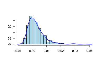
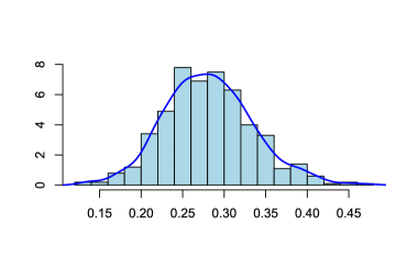
(A): Empirical distribution of $\mathrm{gCov}_{n}$ under $H_{0}$	(B): Empirical distribution of $\mathrm{gCov}_{n}$ under $H_{1}$

Figure 1: Empirical distribution of $\mathrm{gCov}_{n}$ under $H_{0}$ and $H_{1}$. In the univariate setting $p=q=1$, the number of nodes $n$ is 500, the kernel function of $G_{1}$ is a Gaussian kernel, and the kernel function of $G_{2}$ is a Laplace kernel. Under the null hypothesis, the latent variable $X$ follows a beta distribution with parameters $\alpha=1$ and $\beta=2$, and $Y$ follows a standard normal distribution. Under the alternative hypothesis, the latent variable $X$ follows a beta distribution with $\alpha=1$ and $\beta=2$, and $Y$ has a linear relationship with $X$. The histogram of empirical $\mathrm{gCov}_{n}$ is obtained by computing 500 independent cases.

3.4.  Permutation Test

We use the permutation test to test the independence of a pair of random graphs (Nichols and Holmes, 2002). The permutation test procedure can approximate the distribution of a test statistic under the null hypothesis by randomly permuting the dataset, and this method is used in many studies (Shen et al., 2019; Lee et al., 2019; Xiong et al., 2019). Next, we discuss the calculation steps and prove the testing consistency of $\mathrm{gCov}$.

The latent position random graphs $G_{1}$ and $G_{2}$ are generated by latent variables $\mathbf{X}$ and $\mathbf{Y}$, respectively. We used the eigendecomposition of the adjacency matrix to estimate the latent position and denoted as $\hat{\mathbf{X}}$ and $\hat{\mathbf{Y}}$. The initial sample $\mathrm{gCor}$ statistic is calculated by $\hat{\mathbf{X}}$ and $\hat{\mathbf{X}}$ and denoted by $\mathrm{gCor}_{n}^{0}(G_{1},G_{2})$. Then shuffle the order of $\hat{\mathbf{Y}}$, record it as $\hat{\mathbf{Y}}^{*}$, calculate the sample $\mathrm{gCor}$ and record it as $\mathrm{gCor}_{n}^{*}(G_{1},G_{2})$. The permutation step is repeated $r$ times, and the following probability obtains the p-value estimate

$$Pr\left\{\mathrm{gCor}_{n}^{*}(G_{1},G_{2})>\mathrm{gCor}_{n}^{0}(G_{1},G_{2})\right\}.$$

The null hypothesis is rejected if the calculated p-value is less than a pre-specified critical level, usually set to 0.05 or 0.01. The following theorem states that the p-value obtained by the permutation test method is valid for testing the independence of random graphs using $\mathrm{gCor}$.

Theorem 5.

Suppose two latent position random graphs $G_{1}$ and $G_{2}$ are generated by latent variables $\mathbf{X}$ and $\mathbf{Y}$, respectively. Given the Type I error level $\alpha>0$, the sample $\mathrm{gCor}$ is a valid test statistic under the permutation test.

4.  Some Extentions

4.1.  Maximum Mean Discrepancy for Independence Test

In this section, we will introduce the maximum mean discrepancy and use it to illustrate the difference and connection between the independence test of the network and the traditional two-sample test problem of the random graph.

Assume $X\sim F_{X}$ and $Y\sim F_{Y}$, where $F_{X}$, $F_{Y}$ are two Borel probability measures defined on a domain $\mathcal{X}$. The definition of maximum mean discrepancy is as follows.

Definition 3 (Maximum Mean Discrepancy (MMD)).

Let $\mathcal{F}$ denotes the set of measurable functions $f$, then the MMD is defined as

$$\mathrm{MMD}(\mathcal{F},F_{X},F_{Y}) :=\underset{f\in\mathcal{F}}{\mathrm{sup}}\left|\int fdF_{X}-\int fdF_{Y}\right|$$

$$=\underset{f\in\mathcal{F}}{\mathrm{sup}}\left|\mathrm{E}_{x}\left[f(x)\right]-\mathrm{E}_{y}\left[f(y)\right]\right|.$$

In (Müller, 1997), this metric can also be called the integral probability metric.

According to the properties in the RKHS, (Gretton et al., 2006) proposed the maximum mean discrepancy for the two-sample test problem in kernel space. The kernel mean of $X$ is defined as follows:

$$\mu_{X}=\int K(x,\cdot)dF_{X}(x)=E_{X}K(X,\cdot),$$

The kernel mean of $Y$ is also similar. Then the MMD can be represented by the norm of kernel mean, as the Lemma 4 in (Gretton et al., 2006).

$$\mathrm{MMD}(\mathcal{F},F_{X},F_{Y})=\underset{\left\|f\right\|_{\mathcal{H}}\leq 1}{\mathrm{sup}}\left\langle\mu_{X}-\mu_{Y},f\right\rangle_{\mathcal{H}}=\left\|\mu_{X}-\mu_{Y}\right\|_{\mathcal{H}}.$$

The traditional two-sample hypothesis testing problem of random graphs aims to see whether two random graphs have similar structures. That is, whether the latent positions that generate the probability matrix are samples from the same distribution, then the null hypothesis is $H_{0}:F_{X}=F_{Y}$. For the MMD we have

$$\mathrm{MMD}(\mathcal{F},F_{X},F_{Y})=0\quad\mathrm{if\ and\ only\ if}\quad F_{X}=F_{Y}.$$

Based on the above conclusions, (Tang et al., 2017) constructed a nonparametric hypothesis testing method to test whether the structures of two random graphs are similar. In the independence test problem for random graphs, the null hypothesis is $H_{0}:F_{XY}=F_{X}F_{Y}$, then we have the following theorem:

Theorem 6.

Suppose two latent position random graphs $G_{1}$ and $G_{2}$ are generated by latent matrices $\mathbf{X}$ and $\mathbf{Y}$, respectively. Then we have

$$\mathrm{MMD}(\mathcal{F},F_{XY},F_{X}F_{Y})=0\quad\mathrm{if\ and\ only\ if}\quad G_{1}\perp G_{2}.$$

Although the traditional two-sample hypothesis testing and independent test in random graphs are two different problems, they can be related by MMD. The difference is the distribution functions compared to MMD.

4.2.  Extension to the normalized Laplacian

The eigendecomposition of Laplacian or the normalized Laplacian matrices can also be used to find feature representations for each node in a random graph. The Laplacian matrix is the discrete form of the Laplace-Beltrami operator, widely used in manifold learning or nonlinear dimension reduction such as Laplacian eigenmaps (Belkin and Niyogi, 2003) and diffusion maps (Coifman and Lafon, 2006).

For the matrix $\mathbf{M}$ with non-negative elements, the normalized Laplacian of matrix $\mathbf{M}$ is defined as follows:

$$\mathbf{\mathcal{L}}(\mathbf{M}):=(\mathrm{diag}(\mathbf{M}\mathbf{1}))^{-1/2}\mathbf{M}(\mathrm{diag}(\mathbf{M}\mathbf{1}))^{-1/2}.$$ (4.1)

We use the definition of the normalized Laplacian matrix in (Tang and Priebe, 2018), which may be slightly different from the normalized Laplacian in some papers, such as denoting it as $\mathbf{I}-\mathbf{\mathcal{L}}(\mathbf{M})$ (Belkin and Niyogi, 2003). For the graph embedding, which uses the eigenvalues and eigenvectors of the normalized Laplacian, the definitions of these two normalized Laplacians are equivalent. Next, we introduce the definition of Laplacian spectral embedding in random graphs.

Definition 4 (Laplacian spectral embedding (LSE)).

Suppose a random graph generated by latent positions $\mathbf{X}\in\mathbb{R}^{n\times p}$ has an adjacency matrix $\mathbf{A}\in\mathbb{R}^{n\times n}$. The normalized Laplacian matrix is $\mathbf{\mathcal{L}}(\mathbf{A})$. Similar to the eigendecomposition of the adjacency matrix, the eigendecomposition of the adjacency matrix’s normalized Laplacian matrix is

$$\mathbf{\mathcal{L}}(\mathbf{A})=\sum_{i=1}^{n}\tilde{\lambda}_{i}\tilde{\mathbf{u}}_{i}\tilde{\mathbf{u}}_{i}^{\mathrm{T}},$$

where $\tilde{\lambda}_{1}\geq\tilde{\lambda}_{2}\geq\cdots\tilde{\lambda}_{n}$ are the eigenvalues and $\tilde{\mathbf{u}}_{1},\cdots,\tilde{\mathbf{u}}_{n}$ are the corresponding eigenvectors. Let $\tilde{\mathbf{S}}_{\mathrm{A}}=\mathrm{diag}\left(\tilde{\lambda}_{1},\tilde{\lambda}_{2},\cdots,\tilde{\lambda}_{d}\right)$, which composed of the first $d$ eigenvalues. $\tilde{\mathbf{U}}_{\mathrm{A}}$ an $n\times d$ matrix composed of the corresponding eigenvectors $\tilde{\mathbf{u}}_{1},\cdots,\tilde{\mathbf{u}}_{d}$. The Lapalcian spectral embedding of $\mathbf{A}$ is $\breve{\mathbf{X}}=\tilde{\mathbf{U}}_{\mathrm{A}}\tilde{\mathbf{S}}_{\mathrm{A}}^{1/2}$.

For the latent position random graph $G=(V,E)$, suppose the kernel matrix $\mathbf{K}$ is generated by the latent positions $\mathbf{X}\in\mathbb{R}^{n\times p}$. Based on the concentration inequality in (Oliveira, 2009), we extend the Lemma 1 into the form of the normalized Laplacian matrix, shown as follows:

Lemma 2.

In the latent position graph with kernel function, let $\tilde{\mathbf{U}}_{\mathrm{A}}\tilde{\mathbf{S}}_{\mathrm{A}}\tilde{\mathbf{U}}_{\mathrm{A}}^{\mathrm{T}}$ be the eigendecomposition of normalized Laplacian matrix $\mathbf{\mathcal{L}}(\mathbf{A})$. The eigendecomposition of $\mathbf{\mathcal{L}}(\mathbf{K})$ is $\tilde{\mathbf{U}}_{\mathrm{K}}\tilde{\mathbf{S}}_{\mathrm{K}}\tilde{\mathbf{U}}_{\mathrm{K}}^{\mathrm{T}}$, let $\tilde{\mathbf{X}}_{n}=\tilde{\mathbf{U}}_{\mathrm{K}}\tilde{\mathbf{S}}_{\mathrm{K}}^{1/2}$. Then for some orthogonal matrix $\mathbf{W}\in\mathbb{R}^{d\times d}$ we have

$$\left\|\breve{\mathbf{X}}_{n}\mathbf{W}-\tilde{\mathbf{X}}_{n}\right\|_{F}\leq 168\delta_{d}^{-2}\sqrt{\frac{d\log{(4n/\eta)}}{\log{n}}},$$ (4.2)

$\delta_{d}$ denotes the quantity $\lambda_{d}-\lambda_{d+1}$ and $\eta$ is a constant in $(0,1/2)$. Let $\breve{\phi}_{d}({\bf x}_{i})$ the i-th row of $\tilde{\mathbf{U}}_{\mathrm{A}}\tilde{\mathbf{S}}_{\mathrm{A}}^{1/2}\mathbf{W}$ and $\tilde{\phi}_{d}({\bf x}_{i})$ the i-th row of $\tilde{\mathbf{U}}_{\mathrm{K}}\tilde{\mathbf{S}}_{\mathrm{K}}^{1/2}$, for $i\in\left[n\right]$ and any $\varepsilon>0$:

$$\mathbb{P}\left(\left\|\breve{\phi}_{d}(X_{i})-\tilde{\phi}_{d}(X_{i})\right\|>\varepsilon\right)\leq 168\delta_{d}^{-2}\varepsilon^{-1}\sqrt{\frac{2d\log{(4n^{3})}}{n\log{n}}}.$$ (4.3)

Lemma 2 indicates that the eigendecomposition of $\mathbf{\mathcal{L}}(\mathbf{A})$ can be used to approximate the eigendecomposition of $\mathbf{\mathcal{L}}(\mathbf{K})$, so we have the following theorem.

Theorem 7.

Suppose two latent position random graphs $G_{1}$ and $G_{2}$ are generated by latent matrices $\mathbf{X}$ and $\mathbf{Y}$, respectively, and the kernel matrices are $\mathbf{K}_{1}$ and $\mathbf{K}_{2}$. Let $\mathbf{A}_{1}$ be the adjacency matrix of $G_{1}$ and $\mathbf{A}_{2}$ be the adjacency matrix of $G_{2}$. The spectral decomposition of $\mathbf{\mathcal{L}}(\mathbf{A}_{1})$ is $\breve{\mathbf{X}}$ and $\mathbf{\mathcal{L}}(\mathbf{A}_{2})$ is $\breve{\mathbf{Y}}$. The spectral decomposition of $\mathbf{\mathcal{L}}(\mathbf{K}_{1})$ is $\tilde{\mathbf{X}}$ and $\mathbf{\mathcal{L}}(\mathbf{K}_{2})$ is $\tilde{\mathbf{Y}}$. Then we have

$$E(\mathrm{dCov}_{n}(\breve{\mathbf{X}},\breve{\mathbf{Y}}))=\mathrm{dCov}_{n}(\tilde{\mathbf{X}},\tilde{\mathbf{Y}})+\mathcal{O}(1/n),$$

$$\mathrm{dCov}_{n}(\breve{\mathbf{X}},\breve{\mathbf{Y}})\overset{n\rightarrow\infty}{\longrightarrow}\mathrm{dCov}_{n}(\tilde{\mathbf{X}},\tilde{\mathbf{Y}}),$$

where $\mathrm{dCov}_{n}$ denotes the sample version of distance covariance.

The above theorem still holds when the Hilbert-Schmidt covariance replaces the distance covariance. Considering the calculation of Hilbert-Schmidt covariance needs to select the kernel function, we choose distance covariance to avoid confusion with the kernel function that generates random graphs. This theorem is still established under the Hilbert-Schmidt covariance.

The spectral decomposition of $\mathbf{\mathcal{L}}(\mathbf{A})$ can only approximate the spectral decomposition of $\mathbf{\mathcal{L}}(\mathbf{K})$. This step can be regarded as the graph embedding of the random graph. Then we can calculate the distance correlation or Hilbert-Schmidt correlation after obtaining lower-dimensional data. Using normalized Laplacian differs from our previous one-step estimation method, a two-step estimation procedure. However, graph embedding is necessary when dealing with random graphs because the direct computation of Euclidean distances in high dimensions ignores the manifold’s topology. This two-step estimation is also widely adopted (Lee et al., 2019), and our theorem above is theoretically proven valid.

4.3.  Extension to Inhomogeneous Random Graphs

We can extend these conclusions to inhomogeneous random graphs (Bollobás et al., 2007). Given the i.i.d latent variable $\left\{X_{i}\right\}_{i=1}^{n}\sim F$, the kernel matrix $\mathbf{K}_{n}=\left\{\rho_{n}K(X_{i},X_{j})\right\}_{i,j=1}^{n}$. The $\rho_{n}\in(0,1)$ is a scaling parameter that makes the random graph sparse, which is more reliable with some practical application scenarios. A common choice for $\rho_{n}$ is $\rho_{n}=(\log{n})/n$ (Bollobás et al., 2007; Oliveira, 2009). We assume the scaling parameter $\rho_{n}$ and the concentration of the random graph satisfies the following two conditions.

• Condition 1. The scaling parameter $\rho_{n}$ satisfies $n\rho_{n}=\omega\left((\log n)^{\frac{1}{2}+\epsilon}\right)$ for $\epsilon>0$. Here the sequence $a_{n}=\omega(b_{n})$ means for any positive constant $C$, there exists $n_{0}$ such that $a_{n}>Cb_{n}$ for all $n\leq n_{0}$.

• Condition 2. Let $\mathbf{A}$ be the adjacency matrix of the inhomogeneous random graph and $E\mathbf{A}$ denotes its expectation. Then we have

  $$\left\|\mathbf{A}-E\mathbf{A}\right\|\leq\sqrt{\log n}$$

  with high probability.

Condition 1 makes the inhomogeneous random graph become a semi-sparse random graph. The semi-sparse random graph also concentrates however, the deviation bound may change. So condition 2 is not very strict. Satisfying the above two conditions, our proposed method for calculating the sample $\mathrm{gCov}_{n}$ can still converge to the population version of $\mathrm{gCov}$, as shown in the following theorem.

Theorem 8.

Suppose two random graphs $G_{1}$ and $G_{2}$ are generated by latent positions $\mathbf{X}\in\mathbb{R}^{n\times p}$ and $\mathbf{Y}\in\mathbb{R}^{n\times q}$, respectively. The scaling parameter is $\rho_{n}$. Each row of $\mathbf{X}$ and $\mathbf{Y}$ are generated i.i.d from $(X,Y)\sim F_{XY}$. The population Hilbert-Schmidt covariance is defined as 2.1. The sample graph covariance is calculated by 3.4. Then we have

$$\mathrm{gCov}_{n}(G_{1},G_{2})\overset{n\rightarrow\infty}{\longrightarrow}\mathrm{gCov}(G_{1},G_{2}).$$

We can see that the main difference between the sparse and dense settings is that the convergence of the sample $\mathrm{gCov}_{n}$ will be affected by the scaling parameter $\rho_{n}$ under the sparse setting. We can also recover concentration after regularization for sparse random graphs, and the effect of regularization remains to explore.

5.  Numerical Studies

5.1.  Simulations

In the numerical simulation section, we verify the convergence of Gcorr and compare the simulation results of Gcorr, MGC, and Dcorr under nine different simulation settings (Székely et al., 2007; Shen et al., 2019; Lee et al., 2019). The first four can be considered linear or approximate linear relationships, and the last five are nonlinear. The specific distributions are shown in the appendix.

Study 1. First, we use two linear relationships to verify that the sample Gcorr will converge to the HSIC directly calculated from the latent position when the number of network nodes increases. The graph’s number of nodes $n$ is from 100 to 5000. Suppose the latent positions $X_{1},\cdots,X_{n}$ are generated from a beta distribution with $\alpha=1$ and $\beta=2$, we consider two linear relationships of $X$ and $Y$: (i) $Y=X$; (ii) $Y=\mathrm{exp}(X)$. Two noise levels are also set for each relationship separately. The kernel functions for generating random graphs are Gaussian kernel $K(x,x^{{}^{\prime}})=\mathrm{exp}(-\frac{(x-x^{{}^{\prime}})^{2}}{\sigma^{2}})$ with $\sigma=1$ and Laplace Kernel $K(y,y^{{}^{\prime}})=\mathrm{exp}(-c\left|y-y^{{}^{\prime}}\right|)$ with $c=1$. For every choice of nodes, we calculate the Gcorr from the embedding dimension $d$ 1 to 5 and get the mean Gcorr. Figure 2 shows that Gcorr converges to the HISC computed directly from the latent positions as the number of nodes increases. Convergence also holds under white noise with variances of 0.05 and 0.1 but may require more nodes. It is worth noting that in practical applications, the latent position cannot be observed and can only be estimated by graph embedding, which also shows the rationality of our estimation method.

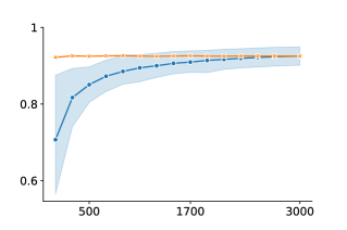
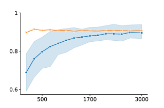
(A): Linear with noise level 0	(B): Exponential with noise level 0
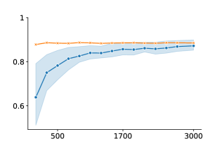
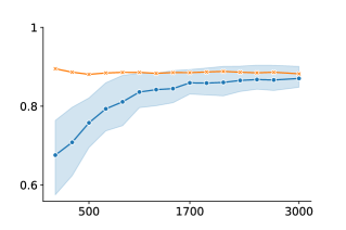
(C): Linear with noise level 0.05	(D): Exponential with noise level 0.05
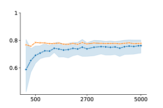
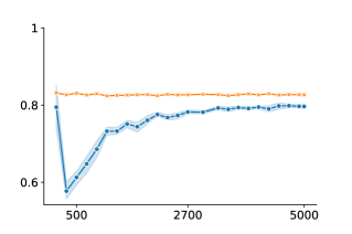
(E): Linear with noise level 0.1	(F): Exponential with noise level 0.1

Figure 2: Simulation results of the sample Gcorr ($\bullet$) and HSIC ($\times$). The left column denotes latent positions $X$, and $Y$ have a linear relationship, and the right column denotes the exponential relationship. The first row results from noise level 0, the second is noise level 0.05, and the third is 0.1. The vertical axis represents the calculated correlation, and the horizontal axis represents the number of graph nodes.

Study 2. Figure 3 shows the sample statistics of Gcorr and MGC for nine correlation settings. For each simulation, we generate a latent position sample $(X,Y)$ at $p=q=1$ and nodes $n=100,500,1500,2000$ with white noise and compare their sample statistics. For the MGC of the random graph, we use the method in (Lee et al., 2019), which uses the eigendecomposition of normalized Laplacian matrix as the sample data. For the dependence relationships (types 1-8), Gcorr and MGC are almost all significantly greater than 0. When the number of nodes in the network is small, Gcorr is considerably higher than MGC, especially in the four nonlinear relationships (types 5-8). As a one-step estimation method, the calculation of Gcorr directly uses the adjacency matrix spectral decomposition to estimate the kernel distance of the latent position. In study 1, we can also see that Gcorr will converge to HSIC of latent position vectors as the number of nodes increases. Although HSIC may not perform as well as MGC in characterizing local correlations, this one-step approach makes estimation more straightforward and interpretable.

Study 3. Figure 4 shows the testing power of Gcorr, MGC and Dcorr under finite samples. Let $p=q=1$ and the number of nodes from 20 to 100 with white noise. We use the following method to estimate the testing power. First, we generate the dependent sample data and calculate the sample statistics, then shuffle the order of $Y$ to generate independent $(X,Y)$ and calculate the new sample statistic. The above process is repeated 1000 times to obtain the p-value, and the testing power is estimated at the Type I error level $\alpha=0.05$ with 100 repetitions. It can be seen that Dcorr does not perform as well as Gcorr and MGC, while the performance of Gcorr and MGC are almost identical in different simulation settings. The testing power reaches 1 when the number of nodes increases to 100, except for the relationship of the W-shape. Therefore, there should be no significant difference between Gcorr and MGC in testing power because the number of nodes is relatively large in the actual data. Since MGC considers local correlations, it is reasonable that the testing power of MGC is better than Dcorr under nonlinear relations. Our method directly estimated the kernel space’s distance, which is also a nonlinear relationship.

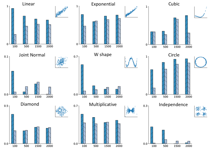
Figure 3: The top right corner is the visualization $(X,Y)$ generated with $n=200$ and $p=q=1$. The bar plot compares sample Gcorr (//) and MGC ($\backslash\backslash$) when the number of nodes is $n=100,500,1500,2000$. The values of the statistics are between 0 and 1, where 0 indicates no relationship. The horizontal axis of the bar plot represents the number of nodes, and the vertical axis represents the sample statistics.

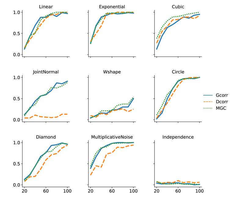
Figure 4: Comparing the testing power of Gcorr, MGC, and Dcorr for nine univariate simulations. The dependent sample data was generated 100 times, and independent data was generated 1000 times. The number of nodes $n$ from 20 to 100 and the Type I error level $\alpha=0.05$. The solid line represents Gcorr, the long dashed line represents Dorr, and the short dashed line represents MGC. The horizontal axis represents the number of nodes, and the vertical axis represents the empirical power.

Study 4.

Figure 5 shows the running time of Gcorr, MGC and Dcorr under finite samples. The p-value of MGC is calculated using the multiscale_graphcorr function of the scipy.stats package in python, the p-value of Dcorr is calculated using the dcor package in python, and Gcorr uses the function written by ourselves, and the timing uses the time package. MGC and Dcorr use a two-step estimation method, first performing eigendecomposition of the normalized Laplacian of the random graph to obtain the low-dimensional vector representation of the random graph and then implementing an independence test between the low-dimensional vectors. Among the three methods, Dcorr is the fastest, MGC is the slowest, and Gcorr runs faster than MGC.

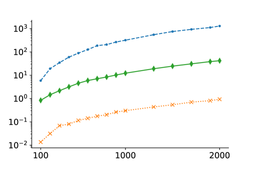
Figure 5: Comparing the running time of Gcorr, MGC, and Dcorr for different nodes. The number of nodes $n$ is from 100 to 2000. The $\blacklozenge$ represents Gcorr, the $\times$ represents Dorr, and the $\bullet$ represents MGC. The horizontal axis represents the number of nodes, and the vertical axis represents the logscale running time.

5.2.  Real Data Analysis

Synaptic connections between neurons play an essential role in understanding the nervous system. The collaboration between neurons can be seen as a complex network through the connection of synapses. While this problem is widely addressed in theory, studying neuronal connections in the existing nervous systems requires electron microscopy, so this method is unsuitable for large structures. The anatomical wiring diagram of the nervous system that has now been fully observed is that of neuronal connections in Caenorhabditis elegans (Jarrell et al., 2012).

The dataset we used is the neuronal connectivity network of the hermaphrodite C. elegans. This data was collected and organized in (Chen et al., 2006; Varshney et al., 2011), and now it can be directly downloaded from https://www.wormatlas.org/neuronalwiring.html#NeuronalconnectivityII. The dataset contains 6417 connections of 280 nonpharyngeal neurons, covering six synaptic connection types: Send or output, Send-poly, Receive or input, Receive-poly, Electric junction, on and Neuromuscular junction. A complete network of neuronal connections in Caenorhabditis elegans can be established by this dataset. In addition, we divide the neurons into two parts that connect the sensory and the muscles of the body. The data used in this step also came from previous studies (White et al., 1986; Dixon and Roy, 2005). Two hundred sensory and motor neurons connect 20 sensory features and 95 body wall muscles. To enrich our study, we subdivided the connections between neurons and muscles into dorsal and ventral body wall muscles. The previously complete network of neuronal connections can be divided into three sub-networks responsible for sensory control, the dorsal body wall muscles and the ventral body wall muscles. Our study aims to explore whether there is a correlation between these three sub-networks. Figure 6 shows the adjacency matrices for these sub-networks.

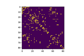
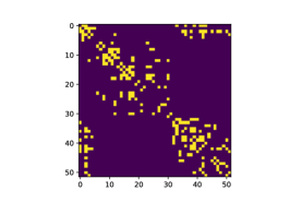
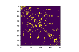
(A): Sensory	(B): Dorsal muscle	(C): Ventral muscle

Figure 6: The adjacency matrices of three sub-networks.

Next, we use the method proposed in this paper to test the network independence between three sub-networks. For the graph correlation, we calculate the three sub-networks pairs: sensory versus the dorsal body wall muscle, sensory versus the ventral body wall muscle, and dorsal body wall muscle versus ventral body wall muscle, respectively. The embedding dimension d is set from 1 to 10. The P value obtained from the permutation test and corresponding graph correlation coefficient are shown in Figure 7. In addition, we set up a control group, that is, the sensory sub-network and a randomly generated Erdös-Rényi model with 80 nodes to test the correlation. Our results show a strong correlation between these three sub-networks; the P values are almost all less than 0.05 under different embedding dimensions.

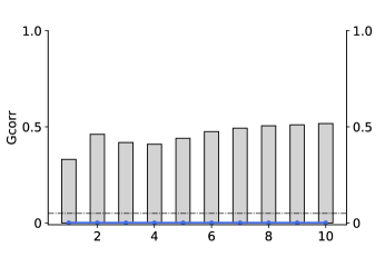
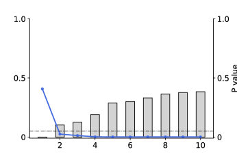
(A): Sensory and Dorsal muscle	(B): Sensory and Ventral muscle
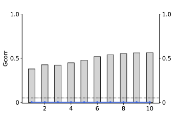
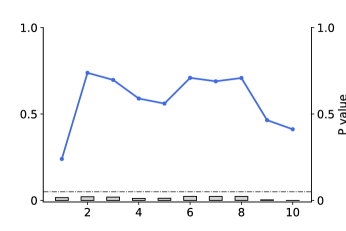
(C): Dorsal muscle and Ventral muscle	(D): Control Group

Figure 7: Comparison of graph correlation coefficients and p-values. The permutation test was repeated $m=1000$. The Bar plot shows the graph correlation coefficient under different embedding dimensions, the solid blue line shows the test p-value, and the gray dotted line denotes the p-value of 0.05.

6.  Discussion

In this paper, we formalized the population version correlation of the latent position random graph, estimated the unbiased sample version by spectral decomposition of the adjacency matrix, and demonstrated convergence from the sample version to the population version. We proved the asymptotic distribution of the sample graph covariance. Numerical simulation confirms that $\mathrm{Gcor}$ performs well in linear and nonlinear dependencies and reduces computational complexity.

There are many potential aspects worthy of further pursuit. For example, our proposed method is based on latent space random graphs. Although we demonstrate that this method can be generalized to inhomogeneous random graphs, the estimation of scaling parameters for inhomogeneous random graphs needs further exploration. In addition, testing random graphs with small nodes displays relatively small testing power, and the choice of embedding dimension may affect the estimation of test statistics. The solution to these problems will further improve the dependence test of the random graph.

SUPPLEMENT TO “RKHS-BASED LATENT POSITION RANDOM GRAPH CORRELATION”

All the proofs for theorems and technical lemmas are involved in A. The simulation dependence functions and subnetwork visualizationin of real data application are in Section B.

Appendix A Proof

Proof of Theorem 1.

Step 1. First, introduce the Mercer’s representation theorem in RKHS, and define the truncated population graph covariance.

From our previous definition, the population graph covariance $\mathrm{hCov}(G_{1},G_{2})$ of two random graphs can be written as

$$\mathrm{hCov}(G_{1},G_{2})=\mathrm{E}\left[K(X,{X}^{\prime})L(Y,{Y}^{\prime})\right]+\mathrm{E}\left[K(X,{X}^{\prime})\right]\mathrm{E}\left[L(Y,{Y}^{\prime})\right]-2\mathrm{E}\left[K(X,{X}^{\prime})L(Y,{Y}^{\prime\prime})\right].$$

Assume we have a compact metric space $(\mathcal{X},d)$ and $\nu$ denotes the strictly positive and finite Borel $\sigma$-field of $\mathcal{X}$. In the calculation equation of $\mathrm{hCov}(G_{1},G_{2})$, the $K:\mathcal{X}\times\mathcal{X}\rightarrow[0,1]$ is continuous and positive definite kernel function. For the dot product $\left\langle\cdot,\cdot\right\rangle$, the RKHS has the following reproducing property:

$$\left\langle f(\cdot),K(x,\cdot)\right\rangle=f(x).$$

Then define the space of square-integrable functions on $\nu$ as $L^{2}(\mathcal{X},\nu)$, the integral operator $T_{K}:L^{2}(\mathcal{X},\nu)\rightarrow L^{2}(\mathcal{X},\nu)$ defined by:

$$T_{K}f:=\int_{\mathcal{X}}K(x,{x}^{\prime})f({x}^{\prime})d\nu({x}^{\prime}),\quad f\in L^{2}(\mathcal{X},\nu).$$

$T_{K}$ is a continuous and compact operator. Let $\left\{\lambda_{i}\right\}$ be the set of eigenvalues of $\mathscr{K}$ and $\lambda_{1}\geq\lambda_{2}\geq\cdots\geq 0$. $\left\{\psi_{i}\right\}$ be the set of corresponding eigenfunctions of $T_{K}$.

Considering the feature mapping of a kernel which takes the form

$$\left\langle\phi(x),\phi({x}^{\prime})\right\rangle_{\mathcal{H}}=K(x,{x}^{\prime}),$$

the Mercer’s representation theorem shows that the feature map $\phi(x)$ can be denoted as

$$\phi(x)=(\sqrt{\lambda_{j}}\psi_{j}(x):j=1,2,\cdots).$$

Let $\phi_{d}(x)$ as the truncation of $\phi(x)$ to $\mathbb{R}^{d}$, where

$$\phi_{d}(x)=(\sqrt{\lambda_{j}}\psi_{j}(x):j=1,2,\cdots,d).$$

Let $K_{d}(x,{x}^{\prime})=\left\langle\phi_{d}(x),\phi_{d}({x}^{\prime})\right\rangle_{\mathcal{H}}$ represents the d-th truncation of the kernel space, and the d-th truncation of $\mathrm{hCov}(G_{1},G_{2})$ is $\mathrm{hCov}^{(d)}(G_{1},G_{2})$, then the truncated population graph covariance can be defined as follows:

$$\mathrm{hCov}^{(d)}(G_{1},G_{2}) =\mathrm{E}\left[K_{d}(X,{X}^{\prime})L_{d}(Y,{Y}^{\prime})\right]+\mathrm{E}\left[K_{d}(X,{X}^{\prime})\right]\mathrm{E}\left[L_{d}(Y,{Y}^{\prime})\right]$$

$$-2\mathrm{E}\left[K_{d}(X,{X}^{\prime})L_{d}(Y,{Y}^{\prime\prime})\right].$$

Step 2. Then we need to show the $\mathrm{hCov}^{(d)}(G_{1},G_{2})$ is equvalent to $\mathrm{hCov}(G_{1},G_{2})$, the proof process refers to (Tang et al., 2013)’s Lemma 3.4. We will use the projection to shows that the subspace spanned by $\phi_{d}$ is equivalent to the subspace spanned by $\phi$.

Let $\mathcal{H}$ be the RKHS induced by kernel function $K$ and define the operators $T_{\mathcal{H}}:\mathcal{H}\rightarrow\mathcal{H}$ and $T_{\mathcal{H},n}:\mathcal{H}\rightarrow\mathcal{H}$ given by:

$$T_{\mathcal{H}}f:=\int_{\mathcal{X}}\left\langle f,K(\cdot,x)\right\rangle_{\mathcal{H}}K(\cdot,x)d\nu(x),$$

$$T_{\mathcal{H},n}f:=\frac{1}{n}\sum_{i=1}^{n}\left\langle f,K(\cdot,x_{i})\right\rangle_{\mathcal{H}}K(\cdot,x_{i}).$$

Assume $\lambda$ is a nonzero eigenvalue of $T_{K}$ and $u$, $v$ are associated eigenfunctions of $T_{K}$ and $T_{\mathcal{H}}$, normalized to norm 1 in $L^{2}(\mathcal{X},\nu)$ and $\mathcal{H}$ respectively, then for $x\in\mathrm{supp}(\nu)$ we have:

$$u(x)=\frac{1}{\sqrt{\lambda}}v(x),\quad v(x)=\frac{1}{\sqrt{\lambda}}\int_{\mathcal{X}}K(x,s)u(s)d\nu(s).$$ (A.1)

The spectra decomposition of kernel matrix $\mathbf{R}$ can be used to estimate the eigenfunction of $T_{K}$. Suppose $\hat{\lambda}$ is a nonzero eigenvalue and $\hat{u}$, $\hat{v}$ are the associated eigenvector and eigenfunction of $\mathbf{R}$ and $T_{\mathcal{H},n}$, normalized to norm 1 in $\mathbb{R}^{n}$ and $\mathcal{H}$ respectively, then:

$$\hat{u}=\frac{1}{\sqrt{\hat{\lambda}}}(\hat{v}(x_{1},\cdots,\hat{v}(x_{n}),\quad\hat{v}(\cdot)=\frac{1}{\sqrt{\hat{\lambda}}}\left(\frac{1}{n}\sum_{i=1}^{n}K(\cdot,x_{i})\hat{u}_{i}\right).$$ (A.2)

Let $\mathcal{P}_{\mathbf{R}}=\mathbf{U}_{\mathbf{R}}\mathbf{U}_{\mathbf{R}}^{\mathrm{T}}$, where $\mathbf{U}_{\mathbf{R}}$ denotes the eigenvectors of kernel matrix $\mathbf{R}=\left\{K(x_{i},x_{j})\right\}_{i,j=1}^{n}$ in graph $G_{1}$. For the samples $X_{1},X_{2},\cdots,X_{n}$, let $\phi_{r,n}\in\mathbb{R}^{n}$ be the vector with elements $\sqrt{\lambda_{r}}\psi_{r}(X_{i})$ for $i=1,2,\cdots,n$, where $\lambda_{r}$ are eigenvalues of $T_{K}$. Then $\mathbf{R}=\sum_{r=1}^{\infty}\phi_{r,n}\phi_{r,n}^{\mathrm{T}}$. Selecting the $d$ largest eigenvalues of $\mathbf{R}$ and denotes the associated eigenvectors as $\hat{u}^{(1)},\cdots,\hat{u}^{(d)}$. We have

$$\left\{\mathcal{P}_{\mathbf{R}}(\mathbf{R})\right\}_{i,j=1}^{n}=\sum_{s=1}^{d}\sum_{r=1}^{\infty}\hat{u}_{i}^{(s)}(\hat{u}^{(s)})^{\mathrm{T}}\phi_{r,n}\phi_{r,n}^{\mathrm{T}}\hat{u}^{(s)}\hat{u}_{j}^{(s)}.$$

For the $\hat{v}^{(1)},\cdots,\hat{v}^{(d)}$ defined in A.2, the following formula is established:

$$\left\langle\hat{v}^{(s)},\sqrt{\lambda_{r}}\psi_{r}\right\rangle_{\mathcal{H}} =\left\langle\frac{1}{\sqrt{\hat{\lambda_{s}}}}\left(\frac{1}{n}\sum_{i=1}^{n}K(\cdot,X_{i})\hat{u}_{i}^{(s)}\right),\sqrt{\lambda_{r}}\psi_{r}\right\rangle_{\mathcal{H}}$$

$$=\frac{1}{\sqrt{\hat{\lambda_{s}}}n}\sum_{i=1}^{n}\psi_{r}(X_{i})\sqrt{\lambda_{r}}\hat{u}_{i}^{(s)}$$

$$=\frac{1}{\sqrt{\hat{\lambda_{s}}}n}\left\langle\hat{u}^{(s)},\phi_{r,n}\right\rangle_{\mathbb{R}^{n}}.$$

Thus we have the following equivalent expression

$$\hat{u}_{i}^{(s)}(\hat{u}^{(s)})^{\mathrm{T}}\phi_{r,n}=\hat{u}_{i}^{(s)}\left\langle\hat{u}^{(s)},\phi_{r,n}\right\rangle_{\mathbb{R}^{n}}=\hat{v}^{(s)}(X_{i})\left\langle\hat{v}^{(s)},\sqrt{\lambda_{r}}\psi_{r}\right\rangle_{\mathcal{H}}.$$

Next, define the $\hat{\mathcal{P}}_{d}$ as the d-dimensional subspace of $T_{K}$, and we have

$$\quad\left\langle\hat{\mathcal{P}}_{d}K(\cdot,X_{i}),\hat{\mathcal{P}}_{d}K(\cdot,X_{j})\right\rangle_{\mathcal{H}}$$

$$=\left\langle\sum_{s=1}^{d}\left\langle\hat{v}^{(s)},K(\cdot,X_{i})\right\rangle_{\mathcal{H}}\hat{v}^{(s)},\sum_{s=1}^{d}\left\langle\hat{v}^{(s)},K(\cdot,X_{i})\right\rangle_{\mathcal{H}}\hat{v}^{(s)}\right\rangle_{\mathcal{H}}$$

$$=\sum_{s=1}^{d}\left\langle\hat{v}^{(s)}(X_{i})\sum_{r=1}^{\infty}\left\langle\hat{v}^{(s)},\sqrt{\lambda_{r}}\psi_{r}\right\rangle_{\mathcal{H}}\sqrt{\lambda_{r}}\psi_{r},\hat{v}^{(s)}(X_{j})\sum_{r=1}^{\infty}\left\langle\hat{v}^{(s)},\sqrt{\lambda_{r}}\psi_{r}\right\rangle_{\mathcal{H}}\sqrt{\lambda_{r}}\psi_{r}\right\rangle_{\mathcal{H}}$$

$$=\sum_{s=1}^{d}\sum_{r=1}^{\infty}\hat{u}_{i}^{(s)}(\hat{u}^{(s)})^{\mathrm{T}}\phi_{r,n}\phi_{r,n}^{\mathrm{T}}\hat{u}^{(s)}\hat{u}_{j}^{(s)}=\left\{\mathcal{P}_{\mathbf{R}}(\mathbf{R})\right\}_{i,j=1}^{n}.$$

The above equations means there exists a matrix $\mathbf{X}\in\mathbb{R}^{n\times d}$ such that $\mathbf{X}\mathbf{X}^{\mathrm{T}}=\mathbf{R}$ and the rows of $\mathbf{X}$ correspond to the projections $\hat{\mathcal{P}}_{d}K(\cdot,X_{i})$. This means the d-dimensional embedding Hilbert space is isometric with $T_{K}$, thus it has distance-preserving property, in that way we can have $\mathrm{hCov}^{(d)}(G_{1},G_{2})=\mathrm{hCov}(G_{1},G_{2})$.

Step 3. Finally, we want to show the sample graph covariance $\mathrm{gCov}_{n}(G_{1},G_{2})$ converges to the truncated population graph covariance.

Let $\hat{K}_{d}(x,{x}^{\prime})=\left\langle\hat{\phi}_{d}(x),\hat{\phi}_{d}({x}^{\prime})\right\rangle_{\mathcal{H}}$, then

$$\left|E\left[K_{d}(x,{x}^{\prime})\right]-E\left[\hat{K}_{d}(x,{x}^{\prime})\right]\right| =\left|\frac{1}{n(n-1)}\sum_{i=1}^{n}\sum_{j\neq i}^{n}K_{d}(x_{i},x_{j})-\frac{1}{n(n-1)}\sum_{i=1}^{n}\sum_{j\neq i}^{n}\hat{K}_{d}(x_{i},x_{j})\right|$$

$$=\left|\frac{1}{n(n-1)}\sum_{i=1}^{n}\sum_{j\neq i}^{n}\left[K_{d}(x_{i},x_{j})-\hat{K}_{d}(x_{i},x_{j})\right]\right|$$

For $K_{d}(x_{i},x_{j})-\hat{K}_{d}(x_{i},x_{j})$:

$$\left|K_{d}(x_{i},x_{j})-\hat{K}_{d}(x_{i},x_{j})\right| =\left|\left\langle\phi_{d}(x_{i}),\phi_{d}(x_{j})\right\rangle_{\mathcal{H}}-\left\langle\hat{\phi}_{d}(x_{i}),\hat{\phi}_{d}(x_{j})\right\rangle_{\mathcal{H}}\right|$$

$$=\left|\left\langle\phi_{d}(x_{i})-\hat{\phi}_{d}(x_{i}),\phi_{d}(x_{j})\right\rangle_{\mathcal{H}}-\left\langle\hat{\phi}_{d}(x_{i}),\phi_{d}(x_{j})-\hat{\phi}_{d}(x_{j})\right\rangle_{\mathcal{H}}\right|$$

$$\leq\left\|\phi_{d}(x_{i})-\hat{\phi}_{d}(x_{i})\right\|\left\|\phi_{d}(x_{j})\right\|+\left\|\hat{\phi}_{d}(x_{i})\right\|\left\|\phi_{d}(x_{j})-\hat{\phi}_{d}(x_{j})\right\|$$

$$\leq C\delta_{d}^{-2}\sqrt{\frac{d\mathrm{log}n}{n}}.$$

Where $C$ is a constant which can bound $\phi_{d}(x_{i})$. The second inequality is obtained by the proof process of Theorem 3.1 in (Tang et al., 2013). Since $K_{d}(x_{i},x_{j})\in\left[0,1\right]$ for $\forall i,j$, then $K_{d}(x_{i},x_{j})$ is uniformly integrable. Then we have:

$$\mathbb{P}(\left|E\left[K_{d}(x,{x}^{\prime})\right]-E\left[\hat{K}_{d}(x,{x}^{\prime})\right]\right|\geq\varepsilon)\rightarrow 0\quad n\rightarrow\infty.$$

Then the proposed $\mathrm{gCov}_{n}(G_{1},G_{2})$ can approximate the d-th truncation of $\mathrm{hCov}(G_{1},G_{2})$, where random graphs are generated by $\mathbf{X}$ and $\mathbf{Y}$.

∎

Proof of Theorem 2.

When $G_{1}$ and $G_{2}$ are independent, the random variables $\left\{X_{i}\right\}_{i=1}^{n}$ and $\left\{Y_{i}\right\}_{i=1}^{n}$ that generate $G_{1}$ and $G_{2}$ are independent.

Considering the Hilbert-Schmidt Independent Criterion (HISC) of random variables X and Y. The Hilbert-Schmidt Independence Criterion is given by

$$\mathrm{HSIC}(p_{xy},\mathcal{F},\mathcal{G}):=\left\|C_{xy}\right\|_{\mathcal{H}}^{2},$$

where $p_{xy}$ denotes the joint measure, random variable $X$ mapped to a reproducing kernel Hilbert space $\mathcal{F}$ and $Y$ mapped to $\mathcal{G}$. $C_{xy}$ denotes the cross-covariance operator. The cross-covariance operator can be calculated by:

$$C_{xy} =\mathrm{E}_{x,y}\left[(f(x)-\mu_{x})\otimes(g(y)-\mu_{y})\right]$$

$$=\mathrm{E}_{x,y}\left[f(x)\otimes g(y)\right]-\mu_{x}\otimes\mu_{y}=\tilde{C}_{xy}-M_{xy}.$$

In the above equations, $\otimes$ denotes the tensor product in Hilbert space. $f(x)$ and $g(y)$ are feature map functions, then $\left\langle f(x),f({x}^{\prime})\right\rangle_{\mathcal{F}}=K(x,{x}^{\prime})$ and $\left\langle g(y),g({y}^{\prime})\right\rangle_{\mathcal{G}}=L(y,{y}^{\prime})$, where $K$ and $L$ are associated kernel functions. Theorem 4 in (Gretton et al., 2005) shows $\left\|C_{xy}\right\|_{\mathcal{H}}=0$ if and only if $x$ and $y$ are independent. Therefore, combined with the definition of $C_{xy}$, the $\mathrm{HSIC}(p_{xy},\mathcal{F},\mathcal{G})$ can be represented in terms of kernel by the definition of the cross-covariance and the relationship between kernel function and feature map:

$$\mathrm{HSIC}(p_{xy},\mathcal{F},\mathcal{G}) =\left\langle\tilde{C}_{xy}-M_{xy},\tilde{C}_{xy}-M_{xy}\right\rangle_{\mathcal{H}}$$

$$=\mathrm{E}\left[\left\langle f(x)\otimes g(y),f(x)\otimes g(y)\right\rangle_{\mathcal{H}}\right]-2\mathrm{E}\left[\left\langle f(x)\otimes g(y),\mu_{x}\otimes\mu_{y}\right\rangle_{\mathcal{H}}\right]$$

$$+\left\langle\mu_{x}\otimes\mu_{y},\mu_{x}\otimes\mu_{y}\right\rangle_{\mathcal{H}}$$

$$=\mathrm{E}\left[K(x,{x}^{\prime})L(y,{y}^{\prime})\right]-2\mathrm{E}\left[K(x,{x}^{\prime})L(y,{y}^{\prime\prime})\right]+\mathrm{E}\left[K(x,{x}^{\prime})\right]\mathrm{E}\left[L(y,{y}^{\prime})\right]$$

Then the independent criterion is equivalent to $\mathrm{hCov}(G_{1},G_{2})=0$ if and only if $G_{1}$ and $G_{2}$ are independent. In the Theorem 1 we proved that $\mathrm{gCov}_{n}(G_{1},G_{2})$ converge to $\mathrm{gCov}(G_{1},G_{2})$ almost surely.

Besides, when $G_{1}$ and $G_{2}$ are independent, $\mathrm{hCov}(G_{1},G_{1})=0$, so $\mathrm{hCor}(G_{1},G_{1})=0$ as well. On the other hand, $\mathrm{hCor}(G_{1},G_{1})>0$ if dependent. Then follows the convergence property of $\mathrm{gCor}_{n}(G_{1},G_{1})$, the proof was completed.

∎

Proof of Theorem 3.

First, we want to obtain the asymptotic distribution of $\mathrm{hCov}_{n}(G_{1},G_{2})$.

Since the U-statistics can be used to estimate $\mathrm{hCov}_{n}(G_{1},G_{2})$. According to Theorem A in Chap 5.5 of (Serfling, 2009), the $\mathrm{hCov}_{n}(G_{1},G_{2})$ is asymptotic normality with mean $\mathrm{hCov}(G_{1},G_{2})$ and variance $\frac{m^{2}}{n}\zeta_{1}$ when $\zeta_{1}\neq 0$. The $\zeta_{c}$ wa defined as follows:

$$\zeta_{c}=E_{F}\left\{\tilde{h}(X_{a_{1}},\cdots,X_{a_{m}})\tilde{h}(X_{b_{1}},\cdots,X_{b_{m}})\right\},$$ (A.3)

where $\tilde{h}(X_{a_{1}},\cdots,X_{a_{m}})=h(X_{a_{1}},\cdots,X_{a_{m}})-\mu$. $c$ represents the number of common elements in sets $\left\{a_{1},\cdots,a_{m}\right\}$ and $\left\{b_{1},\cdots,b_{m}\right\}$. In our estimation procedure, we have $m=4$ and $c=1$. Thus the variance $\sigma_{u}^{2}$ can be written as

$$\sigma_{u}^{2}=16E_{F}\left\{h(X_{a_{1}},\cdots,X_{a_{4}})h(X_{b_{1}},\cdots,X_{b_{4}})-\mathrm{hCov}^{2}\right\}.$$

Known that there is one common element in the two sets $\left\{a_{1},\cdots,a_{4}\right\}$ and $\left\{b_{1},\cdots,b_{4}\right\}$, then we have

$$E_{F}\left\{h(X_{a_{1}},\cdots,X_{a_{4}})h(X_{b_{1}},\cdots,X_{b_{4}})\right\} =(\textrm{C}_{n}^{1})^{-1}\sum_{i=1}^{n}\left\{(\textrm{C}_{n-1}^{4-1})^{-1}\sum_{(j,q,r)\setminus\left\{i\right\}}\frac{1}{3!}h(i,j,q,r)\right\}^{2}$$

$$=\frac{1}{n}\sum_{i=1}^{n}\left\{(n-1)_{3}^{-1}\sum_{(j,q,r)\setminus\left\{i\right\}}h(i,j,q,r)\right\}^{2}=R.$$

where $(n)_{m}=\frac{n!}{(n-m)!}$.

Since $\mathrm{gCov}_{n}(G_{1},G_{2})$ converges to $\mathrm{hCov}_{n}(G_{1},G_{2})$ almost surely, then $\mathrm{gCov}_{n}(G_{1},G_{2})$ also has the same asymptotic normal distribution, which complete the proof.

∎

Proof of Theorem 4.

By the property of the reproducing kernel of the Hilbert space, we can define a centered kernel at probability measure $\nu$ as follows:

$$\bar{K}(x,{x}^{\prime}) :=\left\langle K(x,\cdot)-E_{X}K(X,\cdot),K({x}^{\prime},\cdot)-E_{X}K(X,\cdot)\right\rangle_{\mathcal{H}}$$

$$=K(x,{x}^{\prime})+E_{X{X}^{\prime}}K(X,{X}^{\prime})-E_{X}K(x,X)-E_{X}K({x}^{\prime},X).$$

Since the $\bar{K}(x,{x}^{\prime})$ can also be written as $\bar{K}(x,{x}^{\prime})=\left\langle K(x,\cdot)-\mu_{x},K({x}^{\prime},\cdot)-\mu_{{x}^{\prime}}\right\rangle_{\mathcal{H}}$ by the Bochner integral $\mu_{x}=\int K(x,\cdot)d\nu(x)=E_{X}K(X,\cdot)$. Then we have

$$\mathrm{E}(\bar{K}(x,{x}^{\prime})\bar{L}(y,{y}^{\prime})) =\mathrm{E}\left(\left\langle K(x,\cdot)-\mu_{x},K({x}^{\prime},\cdot)-\mu_{{x}^{\prime}}\right\rangle_{\mathcal{H}}\cdot\left\langle L(y,\cdot)-\mu_{y},L({y}^{\prime},\cdot)-\mu_{{y}^{\prime}}\right\rangle_{\mathcal{H}}\right)$$

$$=\mathrm{E}\left(\left\langle(K(x,\cdot)-\mu_{x})\otimes(L(y,\cdot)-\mu_{y}),(K({x}^{\prime},\cdot)-\mu_{{x}^{\prime}})\otimes(L({y}^{\prime},\cdot)-\mu_{{y}^{\prime}})\right\rangle_{\mathcal{H}}\right)$$

$$=\mathrm{E}\left[\left\langle K(x,\cdot)\otimes L(y,\cdot),K({x}^{\prime},\cdot)\otimes L({y}^{\prime},\cdot)\right\rangle_{\mathcal{H}}\right]-2\mathrm{E}\left[\left\langle K(x,\cdot)\otimes L(y,\cdot),\mu_{x}\otimes\mu_{y}\right\rangle_{\mathcal{H}}\right]$$

$$+\left\langle\mu_{x}\otimes\mu_{y},\mu_{x}\otimes\mu_{y}\right\rangle_{\mathcal{H}}$$

$$=\mathrm{E}\left[K(x,{x}^{\prime})L(y,{y}^{\prime})\right]-2\mathrm{E}\left[K(x,{x}^{\prime})L(y,{y}^{\prime\prime})\right]+\mathrm{E}\left[K(x,{x}^{\prime})\right]\mathrm{E}\left[L(y,{y}^{\prime})\right]$$

$$=\mathrm{hCov}(G_{1},G_{2}).$$

Let $(X^{i},Y^{i})$ be independent for $i\in\left\{1,2,\cdots,6\right\}$. In the (lyons2013distance) introduce the ”core” defined as follows:

$$h((X^{1},Y^{1}),(X^{2},Y^{2}),\cdots,(X^{6},Y^{6})):=f(X^{1},X^{2},X^{3},X^{4})f(Y^{1},Y^{2},Y^{5},Y^{6}),$$

where for $x_{i}\in\mathcal{X}$:

$$f(x_{1},x_{2},x_{3},x_{4}) :=d(x_{1},x_{2})-d(x_{1},x_{3})-d(x_{2},x_{4})+d(x_{3},x_{4})$$

$$=-2\left\{K(x_{1},x_{2})-K(x_{1},x_{3})-K(x_{2},x_{4})+K(x_{3},x_{4})\right\}.$$

The second equation is obtained from the relation in (Sejdinovic et al., 2013) that

$$d(x,{x}^{\prime})=K(x,x)+K({x}^{\prime},{x}^{\prime})-2K(x,{x}^{\prime}).$$

Then, using Fubini’s theorem, we can obtain that:

$$\mathrm{E}\left\{h((X^{1},Y^{1}),\cdots,(X^{6},Y^{6}))\right\} =E\left\{f(X^{1},X^{2},X^{3},X^{4})f(Y^{1},Y^{2},Y^{5},Y^{6})\right\}$$

$$=4\mathrm{E}(\bar{K}(X,{X}^{\prime})\bar{L}(Y,{Y}^{\prime}))=4\mathrm{hCov}(G_{1},G_{2}).$$

Under the null hypothesis, $\mathrm{hCov}(G_{1},G_{2})=0$ since $G_{1}$ and $G_{2}$ are independent, then the kernel $h$ is degenerate of order 1, that is, $\zeta_{1}=0$, where $\zeta_{c}$ is defined in A.3. Then we need to show that $\zeta_{2}\neq 0$. Define the average of kernel $h$ as follows:

$$\bar{h}((X^{1},Y^{1}),\cdots,(X^{6},Y^{6})):=\frac{1}{6!}\sum_{\sigma\in A}h((X^{\sigma(1)},Y^{\sigma(1)}),\cdots,(X^{\sigma(6)},Y^{\sigma(6)})),$$

where $A$ denotes the set of all permutations of $\left\{1,2,\cdots,6\right\}$. Then we have

$$\bar{h}_{2}((x,y),({x}^{\prime},{y}^{\prime})) =\frac{1}{6!}\cdot 2\cdot 4!\cdot h((X^{1},Y^{1}),\cdots,(X^{6},Y^{6}))$$

$$=\frac{4}{15}\mathrm{E}(\bar{K}(X,{X}^{\prime})\bar{L}(Y,{Y}^{\prime})).$$

Therefore the $h((X^{1},Y^{1}),\cdots,(X^{6},Y^{6}))$ has finite second moments. We can use the theory of degenerate U-statistic in Theorem 5.5.2 in (Serfling, 2009) that the $\mathrm{gCov}_{n}(G_{1},G_{2})$ is approximate a chi-square distribution under $H_{0}$.

∎

Proof of Theorem 5.

Define the maps $\tau:\left\{1,2,\cdots,n\right\}\to\left\{1,2,\cdots,n\right\}$ and $\tau_{i}$ will be a permutations of $\left\{1,2,\cdots,n\right\}$ for $i=1,2,\cdots,B$, where $B$ denotes the permutation time. To simplify notation, we denote $\mathrm{gCor}^{*}_{n}(G_{1},G_{2})$ as $\hat{g}(\tau_{i}G)$ and $\mathrm{gCor}^{0}_{n}(G_{1},G_{2})$ as $\hat{g}(G)$. Then we define $R$ as:

$$R=\sum_{i=1}^{B}\mathbbm{1}\left\{\hat{g}(\tau_{i}G)\geq\hat{g}(G)\right\},$$

and reject if $\hat{p}:=\frac{1+R}{1+B}\leq\alpha$, where $\alpha>0$ denotes the Type I erroe level. The finite-sample permutation test has p-value

$$\hat{p}=\frac{1}{B+1}+\frac{1}{B+1}\sum_{i=1}^{B}\mathbbm{1}\left\{\hat{g}(\tau_{i}G)\geq\hat{g}(G)\right\}.$$

When $B$ is large enough, $\hat{p}\leq\alpha$ can be approximated as $\mathbb{P}\left(\hat{g}(\tau_{i}G)\geq\hat{g}(G)\right)\leq\alpha$. Let $d_{n}$ be the number of permutations of $\left\{1,2,\cdots,n\right\}$ that are derangements. Then we have

$$\mathbb{P}\left(\hat{g}(\tau_{i}G)\geq\hat{g}(G)\right)=\mathbb{P}\left(\hat{g}(\tau_{i}G)\geq\hat{g}(G)\mid\tau_{i}=d_{n}\right)\mathbb{P}(\tau_{i}=d_{n})$$

Known that as $n\to\infty$, we have $\mathbb{P}(\tau_{i}=d_{n})\to e^{-1}/d_{n}!$ and $\hat{g}(G)\to\epsilon>0$ under dependence. Thus it suffices to show that for any $\epsilon>0$,

$$\lim_{n\to\infty}e^{-1}\sum_{d_{n}=0}^{n}\mathbb{P}\left(\hat{g}(\tau_{i}G)\geq\epsilon\mid\tau_{i}=d_{n}\right)/d_{n}!\to 0.$$

Given the permutation size $d_{n}$, $G_{1}$ and $G_{2}$ are asymptotically independent, implies $\mathbb{P}\left(\hat{g}(\tau_{i}G)\geq\epsilon\mid\tau_{i}=d_{n}\right)\to 0$ as $n\to\infty$. Then for any $\alpha>0$, there exists $N_{2}>N_{1}$ that for any $d_{n}\leq N_{1}$ and $n>N_{2}$, $\mathbb{P}\left(\hat{g}(\tau_{i}G)\geq\epsilon\mid\tau_{i}=d_{n}\right)<\alpha/2$. Besides, since $\lim_{n\to\infty}\sum_{d_{n}=0}^{n}\frac{1}{d_{n}!}\to e$, we can deduce that $\lim_{n\to\infty}e^{-1}\sum_{d_{n}=N_{1}+1}^{n}\frac{1}{d_{n}!}\leq\alpha/2$. Then for all $n>N_{2}$, we have

$$\quad e^{-1}\sum_{d_{n}=0}^{n}\mathbb{P}\left(\hat{g}(\tau_{i}G)\geq\epsilon\mid\tau_{i}=d_{n}\right)/d_{n}!$$

$$=e^{-1}\sum_{d_{n}=0}^{N_{1}}\mathbb{P}\left(\hat{g}(\tau_{i}G)\geq\epsilon\mid\tau_{i}=d_{n}\right)/d_{n}!+e^{-1}\sum_{d_{n}=N_{1}+1}^{n}\mathbb{P}\left(\hat{g}(\tau_{i}G)\geq\epsilon\mid\tau_{i}=d_{n}\right)/d_{n}!$$

$$\leq e^{-1}\sum_{d_{n}=0}^{N_{1}}\alpha/2d_{n}!+e^{-1}\sum_{d_{n}=N_{1}+1}^{n}1/d_{n}!$$

$$\leq\alpha.$$

Therefore, in the case of $G_{1}$ and $G_{2}$ dependence, for any Type I error level $\alpha>0$, the p-value obtained by the permutation test will be less than $\alpha$ as the sample size $n$ increases. Therefore, the permutation test is consistent for the $\mathrm{gCor}_{n}$ of finite samples. When $G_{1}$ and $G_{2}$ are independent, $\mathrm{gCor}_{n}\to 0$, so $\mathbb{P}\left(\hat{g}(\tau_{i}G)\geq\hat{g}(G)\right)$ is uniformly distributed between 0 and 1, and the permutation test is also valid. ∎

Proof of Theorem 6.

Using the definition of $\mathrm{MMD}(\mathcal{F},F_{XY},F_{X}F_{Y})$, we can have the following equations:

$$\mathrm{MMD}^{2}(\mathcal{F},F_{XY},F_{X}F_{Y}) =\left\|\mu_{XY}-\mu_{X}\otimes\mu_{Y}\right\|_{\mathcal{H}}^{2}$$

$$=\left\langle\mu_{XY}-\mu_{X}\otimes\mu_{Y},\mu_{XY}-\mu_{X}\otimes\mu_{Y}\right\rangle_{\mathcal{H}}$$

$$=\left\langle\mu_{XY},\mu_{XY}\right\rangle_{\mathcal{H}}+\left\langle\mu_{X}\otimes\mu_{Y},\mu_{X}\otimes\mu_{Y}\right\rangle_{\mathcal{H}}-2\left\langle\mu_{XY},\mu_{X}\otimes\mu_{Y}\right\rangle_{\mathcal{H}}$$

$$=\mathrm{E}\left[K(X,{X}^{\prime})L(Y,{Y}^{\prime})\right]+\mathrm{E}\left[K(X,{X}^{\prime})\right]\mathrm{E}\left[L(Y,{Y}^{\prime})\right]$$

$$-2\mathrm{E}\left[K(X,{X}^{\prime})L(Y,{Y}^{\prime\prime})\right]$$

$$=\mathrm{HSIC}(X,Y)=\mathrm{hCov}(G_{1},G_{2}).$$

Thus $\mathrm{MMD}(\mathcal{F},F_{XY},F_{X}F_{Y})=0$ if and only if $G_{1}$ and $G_{2}$ are independent. ∎

Proof of Theorem 7.

The unbiased estimator of sample distance covariance can be calculated by the following formula:

$$\mathrm{dCov}_{n}(X,Y)=\left(\tilde{\mathbf{B}}\cdot\tilde{\mathbf{C}}\right)=\frac{1}{n(n-3)}\sum_{i\neq j}\tilde{b}_{ij}\tilde{c}_{ij},$$

where $\tilde{\mathbf{B}}$ and $\tilde{\mathbf{C}}$ are $\mathcal{U}$-centered matrices of the distance matrices $\mathbf{B}$ and $\mathbf{C}$. Considering the notation $b_{k\cdot}=\sum_{l=1}^{n}b_{kl}$, $b_{\cdot l}=\sum_{k=1}^{n}b_{kl}$ and $b_{\cdot\cdot}=\sum_{k,l=1}^{n}b_{kl}$. The Proposition 1 in (Székely and Rizzo, 2014) shows that the $\left(\tilde{\mathbf{B}}\cdot\tilde{\mathbf{C}}\right)$ can be rewritten as:

$$n(n-3)\left(\tilde{\mathbf{B}}\cdot\tilde{\mathbf{C}}\right)=T_{1}-\frac{T_{2}}{(n-1)(n-2)^{2}}-\frac{2T_{3}}{n-2},$$

where

$$T_{1}=\sum_{k\neq l}b_{kl}c_{kl},\quad T_{2}=b_{\cdot\cdot}c_{\cdot\cdot},\quad T_{3}=\sum_{k}b_{k\cdot}c_{k\cdot}.$$

Let

$$n(n-3)\mathrm{dCov}_{n}(\tilde{\mathbf{X}},\tilde{\mathbf{Y}})=\tilde{T}_{1}-\frac{\tilde{T}_{2}}{(n-1)(n-2)^{2}}-\frac{2\tilde{T}_{3}}{n-2},$$

$$n(n-3)\mathrm{dCov}_{n}(\breve{\mathbf{X}},\breve{\mathbf{Y}})=\breve{T}_{1}-\frac{\breve{T}_{2}}{(n-1)(n-2)^{2}}-\frac{2\breve{T}_{3}}{n-2}.$$

The sepctral decomposition of $\mathbf{\mathcal{L}}(\mathbf{A}_{1})$ is $\breve{\mathbf{X}}$ and $\mathbf{\mathcal{L}}(\mathbf{A}_{2})$ is $\breve{\mathbf{Y}}$, and the spectral decomposition of $\mathbf{\mathcal{L}}(\mathbf{K}_{1})$ is $\tilde{\mathbf{X}}$ and $\mathbf{\mathcal{L}}(\mathbf{K}_{2})$ is $\tilde{\mathbf{Y}}$. let $\breve{X}_{i}$ the i-th row of $\breve{\mathbf{X}}$, $\breve{Y}_{i}$ the i-th row of $\breve{\mathbf{Y}}$, $\tilde{X}_{i}$ the i-th row of $\tilde{\mathbf{X}}$ and $\tilde{Y}_{i}$ the i-th row of $\tilde{\mathbf{Y}}$. Then we have

$$\tilde{T}_{1}-\breve{T}_{1} =\sum_{k\neq l}\left(\left\|\tilde{X}_{k}-\tilde{X}_{l}\right\|\left\|\tilde{Y}_{k}-\tilde{Y}_{l}\right\|-\left\|\breve{X}_{k}-\breve{X}_{l}\right\|\left\|\breve{Y}_{k}-\breve{Y}_{l}\right\|\right)$$

$$=\sum_{k\neq l}(\left\|\tilde{X}_{k}-\tilde{X}_{l}\right\|\left\|\tilde{Y}_{k}-\tilde{Y}_{l}\right\|-\left\|\tilde{X}_{k}-\tilde{X}_{l}\right\|\left\|\breve{Y}_{k}-\breve{Y}_{l}\right\|$$

$$+\left\|\tilde{X}_{k}-\tilde{X}_{l}\right\|\left\|\breve{Y}_{k}-\breve{Y}_{l}\right\|-\left\|\breve{X}_{k}-\breve{X}_{l}\right\|\left\|\breve{Y}_{k}-\breve{Y}_{l}\right\|)$$

$$=l_{1}+l_{2}$$

where

$$l_{1} =\sum_{k\neq l}\left(\left\|\tilde{X}_{k}-\tilde{X}_{l}\right\|\left\|\tilde{Y}_{k}-\tilde{Y}_{l}\right\|-\left\|\tilde{X}_{k}-\tilde{X}_{l}\right\|\left\|\breve{Y}_{k}-\breve{Y}_{l}\right\|\right)$$

$$l_{2} =\sum_{k\neq l}\left(\left\|\tilde{X}_{k}-\tilde{X}_{l}\right\|\left\|\breve{Y}_{k}-\breve{Y}_{l}\right\|-\left\|\breve{X}_{k}-\breve{X}_{l}\right\|\left\|\breve{Y}_{k}-\breve{Y}_{l}\right\|\right).$$

Then we have

$$l_{1} =\sum_{k\neq l}\left(\left\|\tilde{X}_{k}-\tilde{X}_{l}\right\|\left\|\tilde{Y}_{k}-\tilde{Y}_{l}\right\|-\left\|\tilde{X}_{k}-\tilde{X}_{l}\right\|\left\|\breve{Y}_{k}-\breve{Y}_{l}\right\|\right)$$

$$=\sum_{k\neq l}\left\|\tilde{X}_{k}-\tilde{X}_{l}\right\|\left(\left\|\tilde{Y}_{k}-\tilde{Y}_{l}\right\|-\left\|\breve{Y}_{k}-\breve{Y}_{l}\right\|\right)$$

$$=\sum_{k\neq l}\left\|\tilde{X}_{k}-\tilde{X}_{l}\right\|\left(\left\|\tilde{Y}_{k}-\breve{Y}_{k}+\breve{Y}_{k}-\tilde{Y}_{l}\right\|-\left\|\breve{Y}_{k}-\breve{Y}_{l}\right\|\right)$$

$$\leq\sum_{k\neq l}\left\|\tilde{X}_{k}-\tilde{X}_{l}\right\|\left(\left\|\tilde{Y}_{k}-\breve{Y}_{k}\right\|+\left\|\breve{Y}_{k}-\breve{Y}_{l}+\breve{Y}_{l}-\tilde{Y}_{l}\right\|-\left\|\breve{Y}_{k}-\breve{Y}_{l}\right\|\right)$$

$$\leq\sum_{k\neq l}\left\|\tilde{X}_{k}-\tilde{X}_{l}\right\|\left(\left\|\tilde{Y}_{k}-\breve{Y}_{k}\right\|+\left\|\breve{Y}_{l}-\tilde{Y}_{l}\right\|\right).$$

Similarly, we have

$$l_{2}\leq\sum_{k\neq l}\left\|\breve{Y}_{k}-\breve{Y}_{l}\right\|\left(\left\|\tilde{X}_{k}-\breve{X}_{k}\right\|+\left\|\breve{X}_{l}-\tilde{X}_{l}\right\|\right).$$

Then using the results in Lemma 2 we can have the following inequality:

$$\frac{1}{n(n-3)}(\tilde{T}_{1}-\breve{T}_{1})\leq\frac{2}{n(n-3)}2d(n-1)\cdot 168\delta_{d}^{-2}\sqrt{\frac{d\log{(4n/\eta)}}{\log{n}}}\longrightarrow 0$$

as $n\rightarrow\infty$. The rest of $T_{2}$ and $T_{3}$ can also be proved similarly.

∎

Proof of Theorem 8.

For the semi-sparse random graph, we denote the concentration property as

$$\left\|\mathbf{A}-E\mathbf{A}\right\|\leq C$$

Since $E\mathbf{A}=\rho_{n}\mathbf{P}$, then we have

$$\left\|\tilde{\mathbf{A}}-\mathbf{P}\right\|\leq\rho_{n}^{-1}C$$

where $\tilde{\mathbf{A}}=\rho_{n}^{-1}\mathbf{A}$. The eigendecomposition of $\mathbf{P}$ is $\mathbf{U}_{\mathrm{P}}\mathbf{S}_{\mathrm{P}}\mathbf{U}_{\mathrm{P}}^{\mathrm{T}}$, where $\mathbf{U}_{\mathrm{P}}$ composed by the eigenvectors corresponding to the $d$ largest eigenvalues. Let $\mathcal{P}_{\tilde{\mathbf{A}}}=\mathbf{U}_{\mathrm{\tilde{A}}}\mathbf{U}_{\mathrm{\tilde{A}}}^{\mathrm{T}}$ and $\mathcal{P}_{\mathbf{P}}=\mathbf{U}_{\mathrm{P}}\mathbf{U}_{\mathrm{P}}^{\mathrm{T}}$ and $\delta_{d}=\lambda_{d}(\mathcal{K})-\lambda_{d+1}(\mathcal{K})$. The Theorem B.2 in (Tang et al., 2013) shows that with probability at least $1-\eta$, we have

$$\frac{\lambda_{d}(\mathbf{P})}{n}-\frac{\lambda_{d+1}(\mathbf{P})}{n}\geq\delta_{d}-4\sqrt{2}\sqrt{\frac{\log{(2/\eta)}}{n}}.$$

Meanwhile, define the $S_{1}$ and $S_{2}$ as follows:

$$S_{1} =\left\{\lambda:\lambda\geq n\lambda_{d}(\mathbf{P})-\rho_{n}^{-1}C\right\},$$

$$S_{2} =\left\{\lambda:\lambda<n\lambda_{d+1}(\mathbf{P})+\rho_{n}^{-1}C\right\}.$$

Then

$$\mathrm{dist}(S_{1},S_{2})\geq n\delta_{d}-4\sqrt{2}\sqrt{n\log{(2/\eta)}}-2\rho_{n}^{-1}C.$$

Assume $S_{1}$ and $S_{2}$ are disjoint, then we have $\mathrm{dist}(S_{1},S_{2})>0$. According to the $\sin\Theta$ theorem in (davis1970rotation) we have:

$$\left\|\mathcal{P}_{\tilde{\mathbf{A}}}(S_{1})-\mathcal{P}_{\mathbf{P}}(S_{1})\right\| \leq\frac{\left\|\tilde{\mathbf{A}}-\mathbf{P}\right\|}{\mathrm{dist}(S_{1},S_{2})}$$

$$\leq\frac{\rho_{n}^{-1}C}{n\delta_{d}-4\sqrt{2}\sqrt{n\log{(2/\eta)}}-2\rho_{n}^{-1}C}$$

$$\leq\frac{2\rho_{n}^{-1}C}{n\delta_{d}}$$

Since $4\sqrt{2}\sqrt{n\log{(2/\eta)}}+2\rho_{n}^{-1}C\leq n\delta_{d}/2$. Then we have

$$\left\|\mathcal{P}_{\tilde{\mathbf{A}}}(\tilde{\mathbf{A}})-\mathcal{P}_{\mathbf{P}}(\mathbf{P})\right\| \leq\left\|\mathcal{P}_{\tilde{\mathbf{A}}}(\tilde{\mathbf{A}}-\mathbf{P})\right\|+\left\|(\mathcal{P}_{\tilde{\mathbf{A}}}-\mathcal{P}_{\mathbf{P}})\mathbf{P}\right\|$$

$$\leq\rho_{n}^{-1}C+\frac{2\rho_{n}^{-1}C}{\delta_{d}}$$

$$\leq\delta_{d}^{-1}\rho_{n}^{-1}C+2\delta_{d}^{-1}\rho_{n}^{-1}C$$

$$=3\delta_{d}^{-1}\rho_{n}^{-1}C.$$

Having $\mathcal{P}_{\tilde{\mathbf{A}}}=\mathbf{U}_{\mathrm{\tilde{A}}}\mathbf{U}_{\mathrm{\tilde{A}}}^{\mathrm{T}}=\rho_{n}^{-1}\mathbf{U}_{\mathrm{A}}\mathbf{U}_{\mathrm{A}}^{\mathrm{T}}=\rho_{n}^{-1}\mathcal{P}_{\mathbf{A}}$, for some orthogonal matrix $\mathbf{W}\in\mathbb{R}^{d\times d}$, we can obtain the following inequalities:

$$\left\|\rho_{n}^{-1/2}\mathbf{U}_{\mathrm{A}}\mathbf{S}_{\mathrm{A}}^{1/2}\mathbf{W}-\mathbf{U}_{\mathrm{P}}\mathbf{S}_{\mathrm{P}}^{1/2}\right\| \leq\left\|\mathcal{P}_{\tilde{\mathbf{A}}}(\tilde{\mathbf{A}})-\mathcal{P}_{\mathbf{P}}(\mathbf{P})\right\|\frac{\sqrt{d\mathcal{P}_{\tilde{\mathbf{A}}}(\tilde{\mathbf{A}})}+\sqrt{d\mathcal{P}_{\mathbf{P}}(\mathbf{P})}}{\lambda_{d}(\mathbf{P})}$$

$$\leq 3\delta_{d}^{-1}\rho_{n}^{-1}C\frac{2\sqrt{dn}}{\lambda_{d}(\mathbf{P})}\leq 3\delta_{d}^{-1}\rho_{n}^{-1}C\frac{4\sqrt{dn}}{\lambda_{d}(\mathcal{K})}\leq 12\delta_{d}^{-2}\rho_{n}^{-1}C\sqrt{\frac{d}{n}}.$$

Let $\hat{\phi}_{d}(X_{i})$ denotes the i-th column of $\rho_{n}^{-1/2}\mathbf{U}_{\mathrm{A}}\mathbf{S}_{\mathrm{A}}^{1/2}\mathbf{W}$ and $\phi_{d}(X_{i})$ denotes the i-th column of $\mathbf{U}_{\mathrm{P}}\mathbf{S}_{\mathrm{P}}^{1/2}$. Then we have

$$E\left[\left\|\hat{\phi}_{d}(X_{i})-\phi_{d}(X_{i})\right\|\right] \leq\sqrt{E\left[\left\|\hat{\phi}_{d}(X_{i})-\phi_{d}(X_{i})\right\|^{2}\right]}$$

$$\leq\sqrt{\frac{1}{n}E\left[\left\|\rho_{n}^{-1/2}\mathbf{U}_{\mathrm{A}}\mathbf{S}_{\mathrm{A}}^{1/2}\mathbf{W}-\mathbf{U}_{\mathrm{P}}\mathbf{S}_{\mathrm{P}}^{1/2}\right\|_{F}^{2}\right]}$$

$$\leq\frac{1}{\sqrt{n}}\sqrt{(1-\frac{2}{n^{2}})\left(12\delta_{d}^{-2}\rho_{n}^{-1}C\sqrt{\frac{d}{n}}\right)^{2}+\frac{2}{n^{2}}2n}$$

$$\leq 12\delta_{d}^{-2}\rho_{n}^{-1}C\frac{\sqrt{2d}}{n}.$$

Then, by combining the proof process of Theorem 1 and the two conditions, we can derive the following:

$$\mathrm{gCov}_{n}(G_{1},G_{2})\overset{n\rightarrow\infty}{\longrightarrow}\mathrm{gCov}(G_{1},G_{2}).$$

∎

Proof of Lemma 2.

We can rewrite the probability link matrix in the following form for the inhomogeneous random graph:

$$\mathbf{P}=\mathbf{U}_{\mathrm{P}}\mathbf{S}_{\mathrm{P}}\mathbf{U}_{\mathrm{P}}^{\mathrm{T}}=\mathbf{U}_{\mathrm{P}}\mathbf{S}_{\mathrm{P}}^{1/2}(\mathbf{U}_{\mathrm{P}}\mathbf{S}_{\mathrm{P}}^{1/2})^{\mathrm{T}}=\mathbf{X}\mathbf{X}^{\mathrm{T}}.$$

We can rewrite the probability link for the inhomogeneous random graph in the following form. Then the probability link matrix can be expressed as a random dot product graph model under the kernel assumption. The central limit theorem of the Laplacian transform of the random dot product graph model in (Tang and Priebe, 2018) can be directly generalized to a more general model, and we can have $E(\mathbf{\mathcal{L}}(\mathbf{A}))=\mathbf{\mathcal{L}}(\mathbf{P})$.

Then, using the concentration inequality in (Oliveira, 2009), for the normalized Laplacian matrices $\mathbf{\mathcal{L}}(\mathbf{A})$ and $\mathbf{\mathcal{L}}(\mathbf{P})$, with probability at least $1-\eta$, we have

$$\left\|\mathbf{\mathcal{L}}(\mathbf{A})-\mathbf{\mathcal{L}}(\mathbf{P})\right\|\leq 14\sqrt{\frac{\log{(4n/\eta)}}{d_{0}}}\leq 14\sqrt{\frac{\log{(4n/\eta)}}{\log{n}}},$$

where $d_{0}$ is the minimum vertex degree and we suppose $d_{0}\geq C\log{n}$ for some constant $C$.

Similar to $\mathbf{\mathcal{L}}(\mathbf{A})$, the eigendecomposition of $\mathbf{\mathcal{L}}(\mathbf{P})$ is $\tilde{\mathbf{U}}_{\mathrm{P}}\tilde{\mathbf{S}}_{\mathrm{P}}\tilde{\mathbf{U}}_{\mathrm{P}}^{\mathrm{T}}$, where $\tilde{\mathbf{U}}_{\mathrm{P}}$ composed by the eigenvectors corresponding to the $d$ largest eigenvalues. Let $\tilde{\mathcal{P}}_{\mathbf{A}}=\tilde{\mathbf{U}}_{\mathrm{A}}\tilde{\mathbf{U}}_{\mathrm{A}}^{\mathrm{T}}$ and $\tilde{\mathcal{P}}_{\mathbf{P}}=\tilde{\mathbf{U}}_{\mathrm{P}}\tilde{\mathbf{U}}_{\mathrm{P}}^{\mathrm{T}}$ and $\delta_{d}=\lambda_{d}(\mathcal{K})-\lambda_{d+1}(\mathcal{K})$. Like the proof of theorem 8 we have, with probability at least $1-\eta$,

$$\frac{\lambda_{d}(\mathbf{P})}{n}-\frac{\lambda_{d+1}(\mathbf{P})}{n}\geq\delta_{d}-4\sqrt{2}\sqrt{\frac{\log{(2/\eta)}}{n}}.$$

Meanwhile, define the $S_{1}$ and $S_{2}$ as follows:

$$S_{1} =\left\{\lambda:\lambda\geq n\lambda_{d}(\mathbf{P})-14\sqrt{\frac{\log{(4n/\eta)}}{\log{n}}}\right\},$$

$$S_{2} =\left\{\lambda:\lambda<n\lambda_{d+1}(\mathbf{P})+14\sqrt{\frac{\log{(4n/\eta)}}{\log{n}}}\right\}.$$

Then

$$\mathrm{dist}(S_{1},S_{2}) \geq n\delta_{d}-4\sqrt{2}\sqrt{n\log{(2/\eta)}}-28\sqrt{\frac{\log{(4n/\eta)}}{\log{n}}}$$

$$\geq n\delta_{d}-4(\sqrt{2}+7)\sqrt{\frac{n\log{(n/\eta)}}{\log{n}}}.$$

Then we have:

$$\left\|\tilde{\mathcal{P}}_{\mathbf{A}}(S_{1})-\tilde{\mathcal{P}}_{\mathbf{P}}(S_{1})\right\| \leq\frac{\left\|\mathbf{\mathcal{L}}(\mathbf{A})-\mathbf{\mathcal{L}}(\mathbf{P})\right\|}{\mathrm{dist}(S_{1},S_{2})}$$

$$\leq\frac{14\sqrt{\frac{\log{(4n/\eta)}}{\log{n}}}}{n\delta_{d}-4(\sqrt{2}+7)\sqrt{\frac{n\log{(n/\eta)}}{\log{n}}}}\leq 28\sqrt{\frac{\log{(4n/\eta)}}{n\delta_{d}^{2}\log{n}}},$$

provided that $4(\sqrt{2}+7)\sqrt{\frac{n\log{(n/\eta)}}{\log{n}}}\leq n\delta_{d}/2$. Then with probability at least $1-2\eta$,

$$\left\|\tilde{\mathcal{P}}_{\mathbf{A}}-\tilde{\mathcal{P}}_{\mathbf{P}}\right\|\leq 28\sqrt{\frac{\log{(4n/\eta)}}{n\delta_{d}^{2}\log{n}}}.$$

Since $\left\|\mathbf{\mathcal{L}}(\mathbf{A})\right\|\leq n$ and $\left\|\mathbf{\mathcal{L}}(\mathbf{P})\right\|\leq n$ for the normalized Laplacian matrix, we can obtain the following inequalities:

$$\left\|\tilde{\mathcal{P}}_{\mathbf{A}}\mathbf{\mathcal{L}}(\mathbf{A})-\tilde{\mathcal{P}}_{\mathbf{P}}\mathbf{\mathcal{L}}(\mathbf{P})\right\| \leq\left\|\tilde{\mathcal{P}}_{\mathbf{A}}(\mathbf{\mathcal{L}}(\mathbf{A})-\mathbf{\mathcal{L}}(\mathbf{P}))\right\|+\left\|(\tilde{\mathcal{P}}_{\mathbf{A}}-\tilde{\mathcal{P}}_{\mathbf{P}})\mathbf{\mathcal{L}}(\mathbf{P})\right\|$$

$$\leq 14\sqrt{\frac{\log{(4n/\eta)}}{\log{n}}}+28\delta_{d}^{-1}\sqrt{\frac{n\log{(4n/\eta)}}{\log{n}}}\leq 42\delta_{d}^{-1}\sqrt{\frac{n\log{(4n/\eta)}}{\log{n}}}.$$

Then using the Lemma A.1 in (Tang et al., 2013), there exists an orthogonal matrix $\mathbf{W}\in\mathbb{R}^{d\times d}$ such that

$$\left\|\tilde{\mathbf{U}}_{\mathrm{A}}\tilde{\mathbf{S}}_{\mathrm{A}}^{1/2}\mathbf{W}-\tilde{\mathbf{U}}_{\mathrm{P}}\tilde{\mathbf{S}}_{\mathrm{P}}^{1/2}\right\| \leq\left\|\tilde{\mathcal{P}}_{\mathbf{A}}\mathbf{\mathcal{L}}(\mathbf{A})-\tilde{\mathcal{P}}_{\mathbf{P}}\mathbf{\mathcal{L}}(\mathbf{P})\right\|\frac{\sqrt{d\tilde{\mathcal{P}}_{\mathbf{A}}\mathbf{\mathcal{L}}(\mathbf{A})}+\sqrt{d\tilde{\mathcal{P}}_{\mathbf{A}}\mathbf{\mathcal{L}}(\mathbf{P})}}{\lambda_{d}(\mathbf{P})}$$

$$\leq 42\delta_{d}^{-1}\sqrt{\frac{n\log{(4n/\eta)}}{\log{n}}}\frac{2\sqrt{nd}}{\lambda_{d}(\mathbf{P})}=84\delta_{d}^{-1}n\lambda_{d}(\mathbf{P})^{-1}\sqrt{\frac{d\log{(4n/\eta)}}{\log{n}}}.$$

Noted that $\lambda_{d}(\mathbf{P})\geq n\lambda_{d}(\mathcal{K})/2$, then we have

$$\left\|\tilde{\mathbf{U}}_{\mathrm{A}}\tilde{\mathbf{S}}_{\mathrm{A}}^{1/2}\mathbf{W}-\tilde{\mathbf{U}}_{\mathrm{P}}\tilde{\mathbf{S}}_{\mathrm{P}}^{1/2}\right\|_{F}\leq 168\delta_{d}^{-1}\lambda_{d}(\mathcal{K})^{-1}\sqrt{\frac{d\log{(4n/\eta)}}{\log{n}}}\leq 168\delta_{d}^{-2}\sqrt{\frac{d\log{(4n/\eta)}}{\log{n}}}$$

with probability at least $1-2\eta$. Let $\tilde{\phi}_{d}(X_{i})$ denotes the i-th column of $\tilde{\mathbf{U}}_{\mathrm{A}}\tilde{\mathbf{S}}_{\mathrm{A}}^{1/2}\mathbf{W}$ and $\breve{\phi}_{d}(X_{i})$ denotes the i-th column of $\tilde{\mathbf{U}}_{\mathrm{P}}\tilde{\mathbf{S}}_{\mathrm{P}}^{1/2}$. Besides, let $\eta=n^{-2}$ we have

$$E\left[\left\|\tilde{\phi}_{d}(X_{i})-\breve{\phi}_{d}(X_{i})\right\|\right] \leq\sqrt{E\left[\left\|\tilde{\phi}_{d}(X_{i})-\breve{\phi}_{d}(X_{i})\right\|^{2}\right]}$$

$$\leq\sqrt{\frac{1}{n}E\left[\left\|\tilde{\mathbf{U}}_{\mathrm{A}}\tilde{\mathbf{S}}_{\mathrm{A}}^{1/2}\mathbf{W}-\tilde{\mathbf{U}}_{\mathrm{P}}\tilde{\mathbf{S}}_{\mathrm{P}}^{1/2}\right\|_{F}^{2}\right]}$$

$$\leq\frac{1}{\sqrt{n}}\sqrt{(1-\frac{2}{n^{2}})\left(168\delta_{d}^{-2}\sqrt{\frac{d\log{(4n^{3})}}{\log{n}}}\right)^{2}+\frac{2}{n^{2}}2n}$$

$$\leq 168\delta_{d}^{-2}\sqrt{\frac{2d\log{(4n^{3})}}{n\log{n}}}.$$

Then, by Markov’s inequality, for any $\varepsilon>0$ we have

$$\mathbb{P}\left(\left\|\tilde{\phi}_{d}(X_{i})-\breve{\phi}_{d}(X_{i})\right\|>\varepsilon\right)\leq 168\delta_{d}^{-2}\varepsilon^{-1}\sqrt{\frac{2d\log{(4n^{3})}}{n\log{n}}}.$$

∎

Appendix B Simulation functions and Sub-networks

B.1.  Simulation dependence functions

This section presents our nine simulation settings, including four linear relationships, four nonlinear relationships and one independent relationship. Our settings are mainly from the previous work of (Shen et al., 2019), and we have modified some initial distributions and noise values. In this paper, we only consider the simulation results of univariate, that is, $X,Y\in\mathbb{R}$. Besides, $\mathrm{Beta}(a,b)$ denotes the beta distribution with parameters $a$ and $b$, $U(a,b)$ denotes the uniform distribution on the interval $(a,b)$, $N(a,b)$ denotes the normal distribution with mean $a$ and variance $b$ and $B(p)$ denotes the Bernoulli distribution with probability $p$. $\kappa$ is used to control the existence of noise. When there is noise, $\kappa$ equals 1, and 0 otherwise. $c$ represents the variance of the normal distribution, which is used to control the noise level. For example, if the noise level is 0.1, $c$ equals 0.1.

1. Linear $(X,Y)\in\mathbb{R}\times\mathbb{R}$:

   $$X \sim\mathrm{Beta}(1,2),$$

   $$Y =X+\kappa N(0,c).$$

2. Exponential $(X,Y)\in\mathbb{R}\times\mathbb{R}$:

   $$X \sim\mathrm{Beta}(1,2),$$

   $$Y =exp(X)+\kappa N(0,c).$$

3. Cubic $(X,Y)\in\mathbb{R}\times\mathbb{R}$:

   $$X \sim\mathrm{Beta}(1,2),$$

   $$Y =128(X-\frac{1}{3})^{3}+48(X-\frac{1}{3})^{2}-12(X-\frac{1}{3})+\kappa N(0,c).$$

4. Joint normal $(X,Y)\in\mathbb{R}\times\mathbb{R}$:

   $$(X,Y)\sim N(0,\Sigma).$$

   where $\Sigma=\begin{bmatrix}1&0.5\\ 0.5&2\end{bmatrix}$.

5. W shape $(X,Y)\in\mathbb{R}\times\mathbb{R}$:

   $$X \sim\mathrm{Beta}(1,2),$$

   $$Y =4\left\{(X^{2}-\frac{1}{2})^{2}-\frac{1}{500}U(-1,1)\right\}+0.5\kappa N(0,c).$$

6. Circle $(X,Y)\in\mathbb{R}\times\mathbb{R}$, for radius $r=1$ and $\theta=U(0,2\pi)$:

   $$X =r\cos\theta,$$

   $$Y =r\sin\theta+0.5\kappa N(0,c).$$

7. Diamond $(X,Y)\in\mathbb{R}\times\mathbb{R}$, for $u\sim U(-1,1)$, $v\sim U(-1,1)$ and $\theta=-\pi/4$:

   $$X =u\cos\theta+v\sin\theta,$$

   $$Y =-u\sin\theta+v\cos\theta+0.5\kappa N(0,c).$$

8. Multiplicative Noise $(X,Y)\in\mathbb{R}\times\mathbb{R}$, for $u\sim N(0,1)$,

   $$X N(0,1),$$

   $$Y =Xu+0.5\kappa N(0,c).$$

9. Multimodal Independence $(X,Y)\in\mathbb{R}\times\mathbb{R}$, for $u\sim N(0,1)$, $v\sim N(0,1)$, $u_{1}\sim B(0.5)$ and $v_{1}\sim B(0.5)$,

   $$X =u/3+2u_{1}-1,$$

   $$Y =v/3+2v_{1}-1.$$

B.2.  Sub-networks visualization of real data application

In our actual data study, the 280 neurons of Caenorhabditis elegans can be divided into three parts: the neurons controlling the senses, the neurons controlling the dorsal muscles and the neurons controlling the ventral muscles. The interaction of neurons in each area is shown in the figure below.

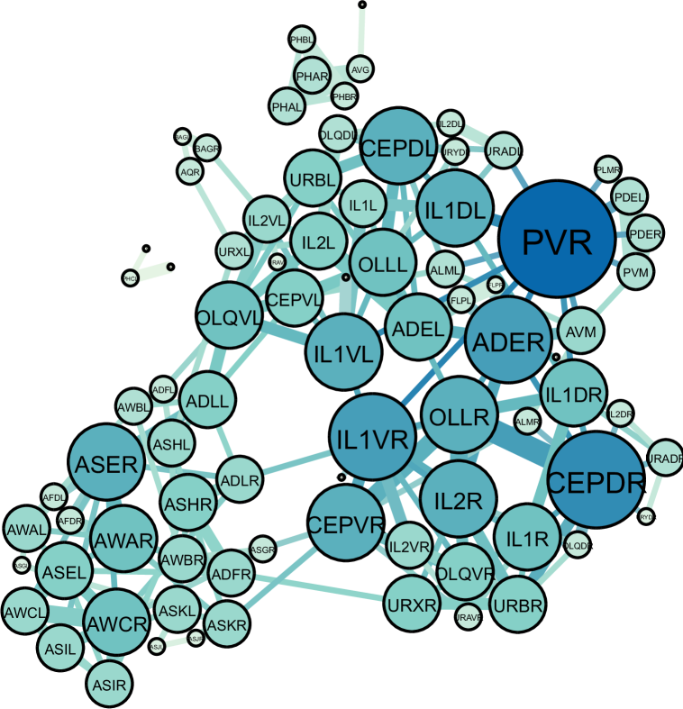
Figure 8: Sub-network for sensory.

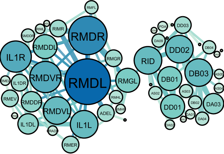
Figure 9: Sub-network for dorsal body wall muscle.

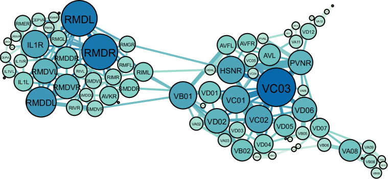
Figure 10: Sub-network for ventral body wall muscle.