Seminormal forms for the Temperley-Lieb algebra.

Abstract

Let ${\mathbb{TL}_{n}^{\!\mathbb{Q}}}$ be the rational Temperley-Lieb algebra, with loop parameter $2$. In the first part of the paper we study the seminormal idempotents $E_{\mathfrak{t}}$ for ${\mathbb{TL}_{n}^{\!\mathbb{Q}}}$ for $\mathfrak{t}$ running over two-column standard tableaux. Our main result is here a concrete combinatorial construction of $E_{\mathfrak{t}}$ using Jones-Wenzl idempotents ${\mathbf{JW}_{\!k}}$ for ${\mathbb{TL}_{k}^{\!\mathbb{Q}}}$ where $k\leq n$.

In the second part of the paper we consider the Temperley-Lieb algebra ${\mathbb{TL}_{n}^{\!{\mathbb{F}}_{p}}}$ over the finite field ${\mathbb{F}}_{\!p}$, where $p>2$. The KLR-approach to ${\mathbb{TL}_{n}^{\!{\mathbb{F}}_{p}}}$ gives rise to an action of a symmetric group $\mathfrak{S}_{m}$ on ${\mathbb{TL}_{n}^{\!{\mathbb{F}}_{p}}}$, for some $m<n$. We show that the $E_{\mathfrak{t}}$’s from the first part of the paper are simultaneous eigenvectors for the associated Jucys-Murphy elements for $\mathfrak{S}_{m}$. This leads to a KLR-interpretation of the $p$-Jones-Wenzl idempotent ${}^{p}\!{\mathbf{JW}_{\!n}}$ for ${\mathbb{TL}_{n}^{\!{\mathbb{F}}_{p}}}$, that was introduced recently by Burull, Libedinsky and Sentinelli.

1   Introduction

In the present paper we introduce a new perspective on both the semisimple and the non-semisimple representation theory of the Temperley-Lieb algebra ${\mathbb{TL}_{n}}$. Some of the ingredients of this new perspective are very classical and well-known, whereas other ingredients are based on ideas developed within the last few couple of years. The unifying element of these ingredients are seminormal forms.

In the representation theory of the symmetric group $\mathfrak{S}_{n}$, the seminormal form has a long history going back to Young’s papers a century ago. A milestone in this history was Murphy’s discovery in the eighties, realizing the seminormal form as common eigenvectors for the Jucys-Murphy elements of the symmetric group. Later on, Mathas showed that Murphy’s results hold in the general framework of a cellular algebra $\mathcal{A}$ endowed with a family of $\mathbf{JM}$-elements. In the present paper we show that ${\mathbb{TL}_{n}}$ fits into this framework, with cellular structure given by the diagram basis and $\mathbf{JM}$-elements induced from the $\mathbf{JM}$-element from the symmetric group.

In Mathas’ framework there is a dichotomy between the ’separated’ and the ’unseparated’ cases and our treatment of ${\mathbb{TL}_{n}}$ follows this dichotomy, with ${\mathbb{TL}_{n}^{\!\mathbb{Q}}}$ corresponding to the separated case and ${\mathbb{TL}_{n}^{\!{\mathbb{F}}_{p}}}$ to the unseparated case. In the separated case, $\mathcal{A}$ is semisimple and there exists a complete set of orthogonal idempotents $\{\mathbb{E}_{\mathfrak{t}}\,|\,\mathfrak{t}\in{\rm Std}(\Lambda)\}$ that are common eigenvectors for the $\mathbf{JM}$-elements. In the unseparated case however, $\mathcal{A}$ is not semisimple and the $\mathbb{E}_{\mathfrak{t}}$’s are undefined, but summing over a $p$-class $[\mathfrak{t}]$ of standard tableaux we have well defined class idempotents in $\mathcal{A}$, given by

$$\mathbb{E}_{[\mathfrak{t}]}:=\sum_{\mathfrak{s}\in[\mathfrak{t}]}\mathbb{E}_{\mathfrak{s}}$$ (1.1)

In general one is especially interested in the primitive idempotents in $\mathcal{A}$, since they correspond to the indecomposable projective modules for $\mathcal{A}$, that carry essential relevant information about the representation theory of $\mathcal{A}$, such as decomposition numbers, etc. The primitive idempotent for the projective cover of the trivial ${\mathbb{TL}_{n}^{\!{\mathbb{F}}_{p}}}$-module, the $p$-Jones-Wenzl idempotent $\,{}^{p}\!{\mathbf{JW}_{\!n}}$, was determined recently by Burull, Libedinsky and Sentinelli in [3], via a recursive construction involving the expansion of $n+1$ in base $p$. The class idempotents $\mathbb{E}_{[\mathfrak{t}]}$ are not always primitive, but in our final Theorem 6.8 we show that ${}^{p}\!{\mathbf{JW}_{\!n}}$ can in fact be built from the class idempotents, via a recursive construction in KLR-theory.

In the separated case, our main results are Theorem 3.7 and Corollary 3.8 that together give a realization of the idempotents $\mathbb{E}_{\mathfrak{t}}$ in terms of a concrete diagrammatic construction involving Jones-Wenzl idempotents ${\mathbf{JW}_{\!k}}$ for ${\mathbb{TL}_{k}^{\!\mathbb{Q}}}$ where $k\leq n$. A key ingredient for the proof of these results is contained in our Theorem 3.3, giving a surprisingly close connection between the Jones-Wenzl idempotents and the seminormal form, in which the well-known recursive formula for ${\mathbf{JW}_{\!n}}$

(1.2)

becomes exactly the classical formula for the action of the symmetric group on the seminormal form, see Corollary 3.4.

Our treatment of the unseparated case ${\mathbb{TL}_{n}^{\!{\mathbb{F}}_{p}}}$ relies heavily on the KLR-algebra (Khovanov-Lauda-Rouquier) approach to ${\mathbb{TL}_{n}^{\!{\mathbb{F}}_{p}}}$. The KLR-algebra was introduced independently by Khovanov-Lauda and Rouquier in [17] and [32], in order to categorify the positive part of the type $A$ quantum group. In seminal papers by Brundan-Kleshchev and Rouquier, see [1] and [32], an isomorphism $\mathcal{R}_{n}\cong{\mathbb{F}}_{\!p}\mathfrak{S}_{n}$ was established (in fact in the greater generality of cyclotomic Hecke algebras). Hu and Mathas gave in [13] a new simpler proof of this isomorphism using seminormal forms, and via this they were able to lift it to an isomorphism ${\mathcal{R}}_{n}^{\mathbb{Z}_{(p)}}\cong\mathbb{Z}_{(p)}\mathfrak{S}_{n}$, where ${\mathcal{R}}_{n}^{\mathbb{Z}_{(p)}}$ is an integral version of ${\mathcal{R}}_{n}$, defined over the localization $\mathbb{Z}_{(p)}$ of $\mathbb{Z}$ at the prime $p$. This isomorphism and its proof is important to us. It firstly induces an isomorphism ${\mathcal{R}}_{n}^{\mathbb{Z}_{(p)}}\!/{\cal I}_{n}\cong{\mathbb{TL}_{n}^{\!{\mathbb{Z}}_{(p)}}}$ where ${\cal I}_{n}$ is an ideal of ${\mathcal{R}}_{n}^{\mathbb{Z}_{(p)}}$, generalizing a result by D. Plaza and the second author, see Theorem 5.3 and [31].

Under the isomorphism ${\mathcal{R}}_{n}^{\mathbb{Z}_{(p)}}\!/{\cal I}_{n}\cong{\mathbb{TL}_{n}^{\!{\mathbb{Z}}_{(p)}}}$, the KLR-generator $e(\mathbf{i})$ for $\mathbf{i}=(0,-1,-2,\ldots,-n+1)$ corresponds to the class idempotent $\mathbf{e}=\mathbb{E}_{[\mathfrak{t}_{n}]}$ where $\mathfrak{t}_{n}$ is the unique one-column standard tableau of length $n$, and so we consider the idempotent truncated subalgebra $\mathbf{e}{\mathbb{TL}_{n}^{\!{\mathbb{Z}}_{(p)}}}\mathbf{e}$ of ${\mathbb{TL}_{n}^{\!{\mathbb{Z}}_{(p)}}}$. It contains block intertwining elements $\mathbb{U}_{i}$, that are represented diagrammatically by ’diamonds’ as follows, for $p=3$.

$$\mathbb{U}_{1}=\raisebox{-0.5pt}{\includegraphics[scale={0.75}]{dib76.pdf}} \mathbb{U}_{2}=\raisebox{-0.5pt}{\includegraphics[scale={0.75}]{dib77.pdf}}$$ (1.3)

Similar elements have been already been considered before for example in [18], [19], [20] and [21], but only in the context of the original KLR-algebra $\mathcal{R}_{n}$ defined over a field.

Our main results in the unseparated case revolve around the action of the $\mathbb{U}_{i}$’s on the seminormal form for ${\mathbb{TL}_{n}^{\!\mathbb{Q}}}$, given by Hu-Mathas’ isomorphism. The key result is our Theorem 6.1, which establishes a formula reminiscent of the classical formula for the action of the symmetric group on Young’s seminormal form. The fact that such a formula is possible in the representation theory of ${\mathbb{TL}_{n}^{\!{\mathbb{Z}}_{(p)}}}$, and hence also of ${\mathbb{TL}_{n}^{\!{\mathbb{F}}_{p}}}$, is highly surprising, and could surely not have been conceived before the introduction of KLR-algebra in representation theory, in particular before Hu-Mathas’ proof of the isomorphism ${\mathcal{R}}_{n}^{\mathbb{Z}_{(p)}}\cong\mathbb{Z}_{(p)}\mathfrak{S}_{n}$.

As a first consequence of Theorem 6.1 we obtain in Corollary 6.9 an injection $\iota_{KLR}:{\mathbb{TL}}_{n_{2}}^{\!{\mathbb{Z}}_{(p)}}\rightarrow{\mathbb{TL}}_{n}^{\!{\mathbb{Z}}_{(p)}}$ for $n_{2}$ a concretely given number $n_{2}<n$. The small Temperley-Lieb algebra ${\mathbb{TL}}_{n_{2}}^{\!{\mathbb{Z}}_{(p)}}$ is of course endowed with its own $\mathbf{JM}$-elements $\textswab{L}_{i}$, with associated seminormal form idempotents $\{\mathbf{E}_{s}\}$ that apriori are unrelated to the original seminormal form idempotents $\{\mathbb{E}_{\mathfrak{t}}\}$ for ${\mathbb{TL}_{n}^{\!\mathbb{Q}}}$. But nevertheless we establish in Theorem 6.5, Corollary 6.6 and Corollary 6.7 another series of surprising facts, showing that the $\mathbb{E}_{\mathfrak{t}}$’s are eigenvectors for the $\textswab{L}_{i}$’s, and that the product $\mathbf{E}_{\mathfrak{s}}\mathbb{E}_{\mathfrak{t}}$ is given by a simple formula.

These last results are the essence of our recursive construction of ${}^{p}\!{\mathbf{JW}_{\!n}}$, We obtain a chain

$$0\subseteq{\mathbb{TL}}_{n^{k-1}_{2}}^{\!{\mathbb{Z}}_{(p)}}\subseteq{\mathbb{TL}}_{n^{k-2}_{2}}^{\!{\mathbb{Z}}_{(p)}}\subseteq\cdots\subseteq{\mathbb{TL}}_{n_{2}^{0}}^{\!{\mathbb{Z}}_{(p)}}={\mathbb{TL}}_{n}^{\!{\mathbb{Z}}_{(p)}}$$ (1.4)

of subalgebras, and let $\mathbf{E}_{[\mathfrak{t}_{n^{i}_{2}}]}$ be the class idempotent for ${\mathbb{TL}}_{n_{2}^{i}}^{\!{\mathbb{Z}}_{(p)}}$, considered as element of ${\mathbb{TL}}_{n}^{\!{\mathbb{Z}}_{(p)}}$. In our final Theorem 6.8 we show that $\,{}^{p}\!{\mathbf{JW}_{\!n}}$ is the product of these $\mathbf{E}_{[\mathfrak{t}_{n^{i}_{2}}]}$’s.

The organization of our paper is as follows. In section 2 we fix notation and recall some basic results concerning the objects that are studied in the paper, that is the Temperley-Lieb algebra ${\mathbb{TL}_{n}}$, the group algebra of the symmetric group, and so on. In section 3, we construct for each two-column standard tableau $\mathfrak{t}$ an element $\mathbb{E}_{\mathfrak{t}}^{\prime}\in{\mathbb{TL}_{n}^{\!\mathbb{Q}}}$ and show that $\mathbb{E}_{\mathfrak{t}}^{\prime}=\mathbb{E}_{\mathfrak{t}}$. In section 4, we initiate our study of the unseparated case. We recall the construction of $\,{}^{p}\!{\mathbf{JW}_{\!n}}$ and give various examples that motivate and illustrate the main results of the last section. In section 5, we recall the KLR algebra $\mathcal{R}_{n}$ and in particular Hu and Mathas’ integral version ${\mathcal{R}}_{n}^{\mathbb{Z}_{(p)}}$ of $\mathcal{R}_{n}$. We also recall the basic ingredients in Hu and Mathas’ proof of the isomorphism ${\mathcal{R}}_{n}^{\mathbb{Z}_{(p)}}\cong\mathbb{Z}_{(p)}\mathfrak{S}_{n}$. They involve a series of formulas for the action of the KLR-generators on the seminormal basis.

In section 6, we prove our main results concerning the unseparated case, starting with Theorem 6.1, which describes the action of the $\mathbb{U}_{i}$ on the seminormal basis. We found the results of this section with considerable aid from the Sage computer system. The proof of Theorem 6.1 is a lengthy calculation involving Hu-Mathas’ formulas. We firmly believe that it is possible to generalize all our results of the present paper to hold for the Tempeley-Lieb algebra at loop parameter $q+q^{-1}$ and have in fact already made some progress in this direction. On the other hand, we also realized that the generalization of Theorem 6.1 to loop parameter $q+q^{-1}$ involves substantially more calculations and we therefore decided to develop our results firstly in the loop parameter 2 setting.

We thank N. Libedinsky, D. Plaza and S. Griffeth for useful comments on a previous version of this work. We specially thank G. Burull for explaining us the construction of ${}^{p}\!{\mathbf{JW}_{\!n}}$.

2   Basic notions

In this section we fix notation and recall the basic notions related to the symmetric group and Temperley-Lieb algebra and their representation theories.

Let $n$ be a positive integer. A partition of $n$ of length $k$ is a weakly decreasing sequence $\lambda=(\lambda_{1},\lambda_{2},\ldots,\lambda_{k})$ of positive integers with total sum $n$. The set of partitions of $n$ is denoted ${\rm Par}_{n}$. A partition $\lambda=(\lambda_{1},\lambda_{2},\ldots,\lambda_{k})\in{\rm Par}_{n}$ is represented diagrammatically by its Young diagram, which consists of $k$, left aligned, rows of nodes with $\lambda_{1}$ nodes in the first row, $\lambda_{2}$ nodes in the second row, and so on. For example, $\lambda=(7,4,2^{2})=(7,4,2,2)\in{\rm Par}_{15}$ is represented by the following Young diagram

$$\lambda=\raisebox{-0.5pt}{\includegraphics[scale={0.7}]{dib47.pdf}}$$ (2.1)

As in (2.1), we shall identify $\lambda\in{\rm Par}_{n}$ with its Young diagram. The set of partitions of $n$ whose Young diagram has less than two columns is denoted ${\rm Par}_{n}^{\leq k}$. For $\lambda,\mu\in{\rm Par}_{n}$ we write $\lambda\trianglelefteq\mu$ if $\lambda_{1}\leq\mu_{1}$, $\lambda_{1}+\lambda_{2}\leq\mu_{1}+\mu_{2}$, $\lambda_{1}+\lambda_{2}+\lambda_{3}\leq\mu_{1}+\mu_{2}+\mu_{3}$, and so on. This is the dominance order on ${\rm Par}_{n}$. For $\lambda\in{\rm Par}_{n}$, a $\lambda$-tableau $\mathfrak{t}$ is a filling of the nodes of the Young diagram of $\lambda$ using the numbers from the set $\{1,2,\ldots,n\}$, with each number occurring once. A $\lambda$-tableau $\mathfrak{t}$ is said to be standard if the numbers from $\{1,2,\ldots,n\}$ appear increasingly from left to right along the rows of $\lambda$, and increasing from top to bottom along the columns of $\lambda$. The set of standard $\lambda$-tableaux is denoted ${\rm Std}(\lambda)$. Here is an example of a standard $\lambda$-tableau $\mathfrak{t}$, for $\lambda$ as in (2.1)

$$\mathfrak{t}=\raisebox{-0.5pt}{\includegraphics[scale={0.7}]{dib48.pdf}}$$ (2.2)

We define $\text{shape}(\mathfrak{t})=\lambda$ if $\mathfrak{t}\in{\rm Std}(\lambda)$. For $\mathfrak{t}$ any standard tableau we define $\mathfrak{t}|_{\leq m}$ to be the tableau obtained from $\mathfrak{t}$ by deleting all the nodes that contain numbers strictly larger than $m$. We then extend the dominance order to standard tableaux via $\mathfrak{s}\trianglelefteq\mathfrak{t}$ if $\text{shape}(\mathfrak{s}|_{\leq m})\trianglelefteq\text{shape}(\mathfrak{t}|_{\leq m})$ for all $m=1,2,\ldots,n$.

For $\lambda\in{\rm Par}_{n}$ we define $\mathfrak{t}^{\lambda}\in{\rm Std}(\lambda)$ as the row-reading tableau, and similarly we define $\mathfrak{t}_{\lambda}\in{\rm Std}(\lambda)$ as the column-reading tableau. When restricted to ${\rm Std}(\lambda)$, we have that $\mathfrak{t}^{\lambda}$ is the unique maximal tableau and $\mathfrak{t}_{\lambda}$ is the unique minimal tableau, with respect to $\trianglelefteq$. For example, for $\lambda$ as in (2.1) we have

$$\mathfrak{t}^{\lambda}=\raisebox{-0.5pt}{\includegraphics[scale={0.7}]{dib49.pdf}},\,\,\,\,\,\,\,\,\mathfrak{t}_{\lambda}=\raisebox{-0.5pt}{\includegraphics[scale={0.7}]{dib50.pdf}}$$ (2.3)

The Temperley-Lieb algebra was introduced in the seventies from motivations in statistical mechanics. In this paper we shall use the variation of the Temperley-Lieb algebra that has loop parameter equal to $2$. It is defined as follows.

Definition 2.1.

The Temperley-Lieb algebra ${\mathbb{TL}_{n}}$ is the associative unitary $\mathbb{Z}$-algebra on generators $\mathbb{u}_{1},\mathbb{u}_{2},\ldots,\mathbb{u}_{n-1}$ subject to the relations

$$\mathbb{u}_{i}^{2} =2\mathbb{u}_{i}, \mbox{if }1\leq i<n$$ (2.4)

$$\mathbb{u}_{i}\mathbb{u}_{j}\mathbb{u}_{i} =\mathbb{u}_{i}, \mbox{if }|i-j|=1$$ (2.5)

$$\mathbb{u}_{i}\mathbb{u}_{j} =\mathbb{u}_{j}\mathbb{u}_{i}, \mbox{if }|i-j|>1$$ (2.6)

For $\Bbbk$ a commutative ring containing a nonzero element $\xi$, we shall also consider the specialized version ${\mathbb{TL}_{n}^{\!\Bbbk}}$ of ${\mathbb{TL}_{n}}$, defined as

$${\mathbb{TL}_{n}^{\!\Bbbk}}:={\mathbb{TL}_{n}}\otimes_{\mathbb{Z}}\Bbbk$$ (2.7)

Here we are mostly interested in the cases where $\Bbbk$ is the rational field $\mathbb{Q}$, the finite field with $p$ elements ${\mathbb{F}}_{\!p}$ or the localization $\mathbb{Z}_{(p)}$ of $\mathbb{Z}$ at the prime $p$, and $\xi=1$. The corresponding Temperley-Lieb algebras are ${\mathbb{TL}_{n}^{\!\mathbb{Q}}}$, ${\mathbb{TL}_{n}^{\!{\mathbb{F}}_{p}}}$ and ${\mathbb{TL}}_{n}^{\!{\mathbb{Z}}_{(p)}}$.

A well-known and important feature of ${\mathbb{TL}_{n}}$ is the fact that it is a diagram algebra. Concretely, ${\mathbb{TL}_{n}}$ is isomorphic to the diagrammatically defined algebra ${\mathbb{TL}_{n}^{\!diag}}$ with basis given by non-crossing planar matchings of $n$ northern points of a(n invisible) rectangle with $n$ southern points of the rectangle. Here are three examples for $n=5$.

(2.8)

We refer to such matchings as Temperley-Lieb diagrams. For two Temperley-Lieb diagrams $D_{1}$ and $D_{2}$ the product $D_{1}D_{2}$ in ${\mathbb{TL}_{n}^{\!diag}}$ is given by concatenation with $D_{1}$ on top of $D_{2}$. For example, choosing $D_{1}$ and $D_{2}$ as the first two diagrams in (2.8) we have that

$$D_{1}D_{2}\,\,=\,\,\raisebox{-0.4pt}{\includegraphics[scale={0.75}]{dib2.pdf}}\,\,=\,\,D_{3}$$ (2.9)

where $D_{3}$ is the third diagram of (2.8). This concatenation product may give rise to diagrams with internal loops. Each internal loop is removed from the diagram, and the resulting diagram is multiplied by the scalar $2\in\mathbb{Z}$. For example, if $D_{1}$ and $D_{3}$ are as above, we have that

$$D_{1}D_{3}\,\,=\,\,\raisebox{-0.4pt}{\includegraphics[scale={0.75}]{dib3.pdf}}\,\,=\,\,2D_{3}$$ (2.10)

The isomorphism between ${\mathbb{TL}_{n}}$ and ${\mathbb{TL}_{n}^{\!diag}}$ is given by

$$\mathbb{1}\,\,\,\,\mapsto\,\,\,\,\raisebox{-0.35pt}{\includegraphics[scale={0.75}]{dib5.pdf}},\,\,\,\mathbb{u}_{i}\,\,\mapsto\,\,\raisebox{-0.35pt}{\includegraphics[scale={0.75}]{dib4.pdf}}$$ (2.11)

where $\mathbb{1}$ is the one-element of ${\mathbb{TL}_{n}}$. From now on we shall identify ${\mathbb{TL}_{n}}$ with ${\mathbb{TL}_{n}^{\!diag}}$ via this isomorphism. There is similar isomorphism for the specialized Temperley-Lieb algebra ${\mathbb{TL}_{n}^{\!\Bbbk}}$ and here we shall also identify ${\mathbb{TL}_{n}^{\!\Bbbk}}$ with the corresponding diagrammatic algebra, defined over $\Bbbk$.

Throughout the paper we shall be interested in the Jones-Wenzl idempotent ${\mathbf{JW}_{\!n}}$ of ${\mathbb{TL}_{n}^{\!\mathbb{Q}}}$. It is the unique nonzero idempotent of ${\mathbb{TL}_{n}^{\!\mathbb{Q}}}$ satisfying

$$\mathbb{u}_{i}{\mathbf{JW}_{\!n}}={\mathbf{JW}_{\!n}}\mathbb{u}_{i}=0\mbox{ for all }i$$ (2.12)

We use the following standard diagrammatic notation for ${\mathbf{JW}_{\!n}}$

$${\mathbf{JW}_{\!n}}=\raisebox{-0.35pt}{\includegraphics[scale={0.7}]{dib6.pdf}}\in{\mathbb{TL}_{n}^{\!\mathbb{Q}}}$$ (2.13)

For example we have that

(2.14)

(2.15)

In general, as one already observes in (2.14) and (2.15), when expanding ${\mathbf{JW}_{\!n}}$ in terms of the diagram basis for ${\mathbb{TL}_{n}^{\!\mathbb{Q}}}$, the coefficient of $\mathbb{1}$ is 1, whereas the other coefficients in general are rational numbers $\dfrac{a}{b}$ with non-trivial denominator. These denominators $b$ prohibit the specialization of ${\mathbf{JW}_{\!n}}$ to fields $\Bbbk$ whose characteristic $p$ divides $b$.

On the other hand, we always have $\mathbf{JW}_{n}^{\ast}={\mathbf{JW}_{\!n}}$ where $\ast$ is the antiautomorphism of ${\mathbb{TL}_{n}^{\!\mathbb{Q}}}$ given by reflection through a horizontal axis, and similarly ${\mathbf{JW}_{\!n}}$ is symmetric with respect to reflection through a vertical axis. These properties can be observed in (2.14) and (2.15).

For general $n$ there is no known closed formula for calculating the coefficients of ${\mathbf{JW}_{\!n}}$ in terms of the diagram basis for ${\mathbb{TL}_{n}^{\!\mathbb{Q}}}$; all known formulas are recursive. We shall need the following recursive formula that goes back to Jones and Wenzl, see [16] and [38].

(2.16)

Combining it with (2.4) we obtain the following well known formula

(2.17)

which can be repeated to arrive at

(2.18)

Using (2.16) one proves that for $m<n$ we have $\mathbf{JW}_{m}\mathbf{JW}_{n}=\mathbf{JW}_{n}$, or diagrammatically

(2.19)

We next recall the basic elements of the representation theory of ${\mathbb{TL}_{n}}$, using the language of cellular algebras. The notion of cellular algebras was introduced by Graham and Lehrer in [7] and in fact ${\mathbb{TL}_{n}}$ was one of their motivating examples.

Definition 2.2.

Let $A$ be an associative $R$-algebra with unit, where $R$ is a commutative ring. A cell datum for $A$ is a triple $(\Lambda,T,C)$ where $\Lambda=(\Lambda,>)$ is a finite poset, $T$ is a function from $\Lambda$ to finite sets and $C$ is an injective function

$$C:\prod_{\lambda\in\Lambda}T(\lambda)\times T(\lambda)\rightarrow A,(s,t)\in T(\lambda)\times T(\lambda)\mapsto C_{st}^{\lambda}$$ (2.20)

These data should satisfy that

1. The image of $C$, that is $im\,C=\{C_{st}^{\lambda}\,|\,(s,t)\in T(\lambda)\times T(\lambda),\lambda\in\Lambda\}$, is an $R$-basis for $A$.

2. For any $a\in A$ we have

   $$C_{st}^{\lambda}a=\sum_{v\in T(\lambda)}r_{tva}C_{sv}^{\lambda}\,\mbox{ mod }A^{\lambda}$$ (2.21)

   where $A^{\lambda}$ is the $R$-submodule of $A$ spanned by $\{C_{st}^{\mu}\,|\,\mu>\lambda\}$.

3. The $R$-linear map $\ast$ of $A$ given by $C_{st}^{\lambda}\mapsto C_{ts}^{\lambda}$ is an algebra anti-isomorphism of $A$.

An algebra endowed with a cell datum $(\Lambda,T,C)$ is called a cellular algebra, with cellular basis $im\,C$.

${\mathbb{TL}_{n}}$ is an example of a cellular algebra. To see this one lets $\Lambda$ be the set of two-column integer partitions ${\rm Par}^{\leq 2}_{n}$, endowed with the usual dominance order, and for $\lambda\in{\rm Par}^{\leq 2}_{n}$ one lets $T(\lambda)$ be the set of standard $\lambda$-tableaux ${\rm Std}(\lambda)$. To explain $C$, one first constructs for $\lambda\in{\rm Par}^{\leq 2}_{n}$ and $\mathfrak{t}\in{\rm Std}(\lambda)$ a Temperley-Lieb half-diagram $C_{\mathfrak{t}}^{\lambda}$ for ${\mathbb{TL}_{n}}$ as follows. Going through the numbers $\{1,2\,\ldots,n\}$ in increasing order, one raises for any $i$ occurring in the first column of $\mathfrak{t}$ a vertical line from the $i$’th lower position of the rectangle and for any $i$ occurring in the second column of $\mathfrak{t}$, one joins the $i$’th lower position with the top end of the first vacant line to the left, always avoiding line crossings. Here is an example for $\lambda=(2^{4},1^{3})\in{\rm Par}_{11}$.

$$\mathfrak{t}:=\raisebox{-0.5pt}{\includegraphics[scale={0.7}]{dib12.pdf}}\mapsto\,\,\,\,C_{\mathfrak{t}}^{\lambda}=\,\raisebox{-0.3pt}{\includegraphics[scale={0.7}]{dib13.pdf}}$$ (2.22)

For a pair of standard $\lambda$-tableaux $(\mathfrak{s},\mathfrak{t})$, one then defines $C_{\mathfrak{s}\mathfrak{t}}^{\lambda}$ as the diagram obtained from $C_{\mathfrak{s}}^{\lambda}$ and $C_{\mathfrak{t}}^{\lambda}$ by reflecting $C_{\mathfrak{s}}^{\lambda}$ horizontally and concatenating below with $C_{\mathfrak{t}}^{\lambda}$. Here is an example.

$$(\mathfrak{s},\mathfrak{t}):=\raisebox{-0.5pt}{\includegraphics[scale={0.7}]{dib14.pdf}}\mapsto\,\,\,\,C_{\mathfrak{s}\mathfrak{t}}^{\lambda}=\,\raisebox{-0.5pt}{\includegraphics[scale={0.7}]{dib15.pdf}}$$ (2.23)

Using the multiplication rules explained in (2.9) and (2.10), one now checks that ${\mathbb{TL}_{n}}$ indeed is a cellular algebra over $\mathbb{Z}$, with the ingredients just introduced, and similarly ${\mathbb{TL}_{n}^{\!\Bbbk}}$ is a cellular algebra over $\Bbbk$.

In general, for a cellular algebra $A$ there is a family of cell modules $\{\Delta(\lambda)\,|\,\lambda\in\Lambda\}$ that play a key role when studying the representation theory of $A$. To define $\Delta(\lambda)$ one chooses an arbitrary $s_{0}\in T(\lambda)$ and sets

$$\Delta(\lambda):={\rm span}_{R}\{C_{s_{0}t}^{\lambda}\,|\,t\in T(\lambda)\}$$ (2.24)

The action of $A$ on $\Delta(\lambda)$ is given by $C_{s_{0}t}^{\lambda}a=\sum_{v\in T(\lambda)}r_{tva}C_{s_{0}v}^{\lambda}$ where $r_{tva}\in R$ is the scalar that appears in (2.21). Note that $\Delta(\lambda)$ is a right module. We shall sometimes write $\Delta^{R}(\lambda)$ for $\Delta(\lambda)$ to indicate the dependence on the ground ring $R$.

In the case of ${\mathbb{TL}_{n}}$, we identify for $\mathfrak{s}_{0},\mathfrak{t}\in{\rm Std}(\lambda)$ the $\Delta(\lambda)$ basis element $C_{\mathfrak{s}_{0}\mathfrak{t}}^{\lambda}$ with the half-diagram $C_{\mathfrak{t}}^{\lambda}$. Under this identification, for a Temperley-Lieb diagram $D$ we have that $C_{\mathfrak{t}}^{\lambda}D$ is the concatenation with $C_{\mathfrak{t}}^{\lambda}$ on top of $D$, where internal loops are removed by multiplying by $2$, and where half-diagrams that do not belong to $\{C_{\mathfrak{t}}^{\lambda}\,|\,\mathfrak{t}\in{\rm Std}(\lambda)\}$ are set equal to zero.

In the present paper, Jucys-Murphy elements play an important role. Their key properties were developed in Murphy’s papers in the eighties, see [26], [27], [28]. These properties were formalized by Mathas as follows, see [25].

Definition 2.3.

Let $A$ be a cellular algebra over $R$ with triple $(\Lambda,T,C)$, and suppose that for each $\lambda\in\Lambda$ there is a poset structure on $T(\lambda)$ with order relation $<$. Then a family of elements $\{L_{1},L_{2},\ldots,L_{M}\}$ is called a set of $\mathbf{JM}$-elements for $A$ if it satisfies the following conditions.

1. The $L_{i}$’s commute and satisfy $L_{i}^{\ast}=L_{i}$.

2. For each $t\in T(\Lambda):=\coprod_{\lambda\in\Lambda}T(\lambda)$ there is a function $c_{t}:\{1,2,\ldots,M\}\rightarrow R$ such that the following triangularity formula holds in $\Delta(\lambda)$

   $$C^{\lambda}_{t}L_{i}=c_{t}(i)C^{\lambda}_{t}+\sum_{s\in T(\lambda),s>t}a_{s}C_{s}^{\lambda}$$ (2.25)

   for some $a_{s}\in R$.

If $\{L_{1},L_{2},\ldots,L_{M}\}$ is a family of $\mathbf{JM}$-elements for $A$, then the corresponding functions $c_{t}$ are called content functions.

$\mathbf{JM}$-elements were first constructed for the group algebra of the symmetric group, and from these one obtains $\mathbf{JM}$-elements for ${\mathbb{TL}_{n}}$, as we shall shortly see.

Let $\mathfrak{S}_{n}$ be the symmetric group of bijections $\{1,2,\ldots,n\}$. For $\sigma\in\mathfrak{S}_{n}$ and $i\in\{1,2,\ldots,n\}$ we write $(i)\sigma$ for the image of $i$ under $\sigma$. This notation reflects our general preference for right actions and right modules over left actions and left modules. We shall use standard cycle notation for elements of $\mathfrak{S}_{n}$, that is $\sigma=(i_{1},i_{2},\ldots,i_{k})$ is the element of $\mathfrak{S}_{n}$ defined by $(i_{1})\sigma=i_{2},(i_{2})\sigma=i_{3},\ldots,(i_{k})\sigma=i_{1}$. For elements $\sigma_{1},\sigma_{2}\in\mathfrak{S}_{n}$ the product $\sigma_{1}\sigma_{2}\in\mathfrak{S}_{n}$ is given by $(i)(\sigma_{1}\sigma_{2})=((i)\sigma_{1})\sigma_{2}$.

Let $\{L_{1},L_{2},\ldots,L_{n}\}\subseteq\mathbb{Z}\mathfrak{S}_{n}\,{(\mbox{or }}\Bbbk\mathfrak{S}_{n})$ be defined by

$$L_{1}:=0,\mbox{ and }L_{i}:=(1,i)+(2,i)+\ldots+(i-1,i)\mbox{ for }i=2,3,\ldots,n$$ (2.26)

Define moreover for $\mathfrak{t}\in{\rm Std}(\lambda)$ the function $c_{\mathfrak{t}}:\{1,2,\ldots,n\}\rightarrow\mathbb{Z}\,{(\mbox{or }}\Bbbk)$ by

$$c_{\mathfrak{t}}(i):=c-r\mbox{ for }\mathfrak{t}[r,c]=i$$ (2.27)

where $\mathfrak{t}[r,c]$ is the number that appears in the $r$’th row of $\mathfrak{t}$, counted from top to bottom, and in the $c$’th column of $\mathfrak{t}$, counted from the left to right.

$\mathfrak{S}_{n}$ is a Coxeter group on the simple transpositions $s_{i}:=(i,i+1)$. We need the following well known fundamental Lemma, which is easily verified.

Lemma 2.4.

There is a surjection $\Phi:\mathbb{Z}\mathfrak{S}_{n}\rightarrow{\mathbb{TL}_{n}}$, given by $s_{i}\mapsto\mathbb{u}_{i}-\mathbb{1}$. The kernel of $\Phi$ is the ideal in $\mathbb{Z}\mathfrak{S}_{n}$ generated by $s_{1}s_{2}s_{1}+s_{1}s_{2}+s_{2}s_{1}+s_{1}+s_{2}+1$. A similar statement holds over $\Bbbk$.

Let $\mathbf{L}_{i}:=\Phi(L_{i})$. We represent $\mathbf{L}_{i}$ diagrammatically as follows

$$\mathbf{L}_{i}=\raisebox{-0.35pt}{\includegraphics[scale={0.7}]{dib36.pdf}}$$ (2.28)

We now have the following key result.

Theorem 2.5.

$\{\mathbf{L}_{1},\mathbf{L}_{2},\ldots,\mathbf{L}_{n}\}$ is a family of $\mathbf{JM}$-elements for ${\mathbb{TL}_{n}}$ with respect to the content functions $c_{\mathfrak{t}}$, defined in (2.27).

Proof: $\{L_{1},L_{2},\ldots,L_{n}\}$ is known to be a family of $\mathbf{JM}$-elements for the cellular structure on $\mathbb{Z}\mathfrak{S}_{n}$ given by the specialization $q=1$ of Murphy’s standard basis for the Hecke algebra, see [24] and [28]. On the other hand, $\Phi:\mathbb{Z}\mathfrak{S}_{n}\rightarrow{\mathbb{TL}_{n}}$ maps the standard basis cellular structure on $\mathbb{Z}\mathfrak{S}_{n}$ to the diagram basis cellular structure on ${\mathbb{TL}_{n}}$ and therefore $\{\mathbf{L}_{1},\mathbf{L}_{2},\ldots,\mathbf{L}_{n}\}$ is a family of $\mathbf{JM}$-elements for ${\mathbb{TL}_{n}}$, as claimed. For more details one should consult [30].   $\square$

3   The separated case

In this section we consider the rational Temperley-Lieb algebra ${\mathbb{TL}_{n}^{\!\mathbb{Q}}}$. The ground ring for ${\mathbb{TL}_{n}^{\!\mathbb{Q}}}$ is $\mathbb{Q}$ which implies that for two-column partitions $\lambda$ and $\mu$ and for standard tableaux $\mathfrak{s}\in{\rm Std}(\lambda)$ and $\mathfrak{t}\in{\rm Std}(\mu)$ we have that

$$c_{\mathfrak{s}}(i)=c_{\mathfrak{t}}(i)\mbox{ for }i=1,2,\ldots,n\Longrightarrow\mathfrak{s}=\mathfrak{t}$$ (3.1)

In other words, the separation condition in [25] is fulfilled and so ${\mathbb{TL}_{n}^{\!\mathbb{Q}}}$ is semisimple. The separation condition also implies that the simultaneous action of the $\mathbf{L}_{i}$’s on ${\mathbb{TL}_{n}^{\!\mathbb{Q}}}$ via right multiplication is diagonalizable with eigenvalues given by the $c_{\mathfrak{t}}(i)$’s, and similarly for the left action. Moreover, under the separation condition we have the following expression for the idempotent projector $\mathbb{E}_{\mathfrak{t}}$ for the common eigenvector for all the $\mathbf{L}_{i}$’s with eigenvalues $c_{\mathfrak{t}}(i)$.

$$\mathbb{E}_{\mathfrak{t}}=\prod_{c\in{\cal C}}\,\,\prod_{\begin{subarray}{c}i=1,\ldots,n\\ c\neq c_{\mathfrak{t}}(i)\end{subarray}}\dfrac{\mathbf{L}_{i}-c}{c_{\mathfrak{t}}(i)-c}\in{\mathbb{TL}_{n}^{\!\mathbb{Q}}}$$ (3.2)

where ${\cal C}$ is the set of contents for standard tableaux of two-column partitions, that is

$${\cal C}:=\{c_{\mathfrak{t}}(i)\,|\,i=1,2,\ldots,n\mbox{ and }\mathfrak{t}\in{\rm Std}({\rm Par}^{\leq 2}_{n})\}\,\,\mbox{where}\,\,\,{\rm Std}({\rm Par}^{\leq 2}_{n}):=\bigcup_{\lambda\in{\rm Par}^{\leq 2}_{n}}{\rm Std}(\lambda)$$ (3.3)

With $\mathfrak{t}$ running over ${\rm Std}({\rm Par}^{\leq 2}_{n})$, the $\mathbb{E}_{\mathfrak{t}}$’s form a complete set of orthogonal primitive idempotents for ${\mathbb{TL}_{n}^{\!\mathbb{Q}}}$, that is we have

$$\mathbb{1}=\sum_{\mathfrak{t}\in{\rm Std}({\rm Par}^{\leq 2}_{n})}\mathbb{E}_{\mathfrak{t}},\,\,\,\,\,\mathbf{L}_{i}\mathbb{E}_{\mathfrak{t}}=\mathbb{E}_{\mathfrak{t}}\mathbf{L}_{i}=c_{\mathfrak{t}}(i)\mathbb{E}_{\mathfrak{t}},\,\,\,\,\,\mathbb{E}_{\mathfrak{s}}\mathbb{E}_{\mathfrak{t}}=\delta_{\mathfrak{s}\mathfrak{t}}\mathbb{E}_{\mathfrak{s}}$$ (3.4)

where $\delta_{\mathfrak{s}\mathfrak{t}}$ is the Kronecker delta.

The formulas in (3.2) and (3.4) are consequences of the general theory for $\mathbf{JM}$-elements developed in [25]. For $\mathbb{Q}\mathfrak{S}_{n}$ the analogues of (3.2) and (3.4) were first found by Murphy in [29]. We find it worthwhile to mention that the corresponding properties do not hold for the Young symmetrizer idempotents for $\mathbb{Q}\mathfrak{S}_{n}$, since these are not orthogonal.

The expression for $\mathbb{E}_{\mathfrak{t}}$ given in (3.2) contains many redundant factors and is in general intractable, in the symmetric group case as well as in the Temperley-Lieb case.

The purpose of this section is to give a new expression for $\mathbb{E}_{\mathfrak{t}}$ in the Temperley-Lieb case, using Jones-Wenzl idempotents. In view of this, one may now consider seminormal forms and Jones-Wenzl idempotents as two aspects of the same theory.

Let $\mathfrak{t}\in{\rm Std}(\lambda)$ be a two-column standard tableau. Then $\mathfrak{t}$ can be written in the form

$$\mathfrak{t}=\raisebox{-0.5pt}{\includegraphics[scale={0.75}]{dib16.pdf}}$$ (3.5)

where each $D_{i}$ and $M_{i}$ is a non-empty block of consecutive natural numbers, except that $M_{k}$ is allowed to be empty, satisfying that the numbers of both $D_{i}$ and $M_{i}$ are less than the numbers of both $D_{j}$ and $M_{j}$ if $i<j$. Conversely, each sequence of blocks $D_{1},M_{1},D_{2},\ldots,M_{k}$ satisfying these conditions give rise to a two-column standard tableau $\mathfrak{t}$.

Let $d_{i}:=|D_{i}|$ and $m_{i}=|M_{i}|$ be the cardinalities of $D_{i}$ and $M_{i}$ and define $n_{i}$ for $i=1,2,\ldots,k$ via

$$n_{1}:=d_{1}\mbox{ and }n_{i}=(d_{1}+d_{2}+\ldots+d_{i})-(m_{1}+m_{2}+\ldots+m_{i-1})\mbox{ for }i>1$$ (3.6)

We now associate with $\mathfrak{t}$ an element $f_{\mathfrak{t}}\in\Delta^{\mathbb{Q}}(\lambda)$ in the following recursive way. Suppose first that $M_{k}\neq\emptyset$. If $k=1$ we set

$$f_{\mathfrak{t}}=\raisebox{-0.35pt}{\includegraphics[scale={0.7}]{dib17.pdf}}$$ (3.7)

and if $k=2$ we set

$$f_{\mathfrak{t}}\,\,\,=\,\,\,\raisebox{-0.5pt}{\includegraphics[scale={0.7}]{dib18.pdf}}$$ (3.8)

We repeat this recursively, that is in the $i$’th step we first concatenate on top with $\mathbf{JW}_{\!n_{i}}$ and then bend down the $m_{i}$ top and rightmost lines to the bottom. If $M_{k}=\emptyset$ the construction is the same as for $M_{k}\neq\emptyset$, except that in the last step the bending down of the $m_{k}$ top and rightmost lines is omitted.

For example,

$$\text{if }\mathfrak{t}\,:=\,\raisebox{-0.5pt}{\includegraphics[scale={0.7}]{dib19.pdf}} f_{\mathfrak{t}}\,\,\,=\,\,\,\raisebox{-0.5pt}{\includegraphics[scale={0.6}]{dib20.pdf}}$$ we have that (3.9)

In general, if $i$ appears in the first column of $\mathfrak{t}$ then $i$ is connected in $f_{\mathfrak{t}}$ to the southern border of a Jones-Wenzl element, and if $i$ appears in the second column of $\mathfrak{t}$ then $i$ is connected in $f_{\mathfrak{t}}$ to the northern border of a Jones-Wenzl element. We have indicated this in (3.9), using colors.

In general, for $\mathfrak{t}$ as in (3.5) we shall sometimes represent $f_{\mathfrak{t}}$ in the following schematic way

$$f_{\mathfrak{t}}=\raisebox{-0.5pt}{\includegraphics[scale={0.7}]{dib23.pdf}}$$ (3.10)

where $n$ is a shorthand for ${\mathbf{JW}_{\!n}}$ and where $m_{i}$ indicates the number of lines being bent down, which may be zero for $m_{k}$.

For $\mathfrak{t}$ a two-column standard tableau we set

$$\gamma_{\mathfrak{t}}:=\prod_{j=1}^{k}\dfrac{n_{i}+1}{n_{i}-m_{i}+1}$$ (3.11)

We define $f_{\mathfrak{t}\mathfrak{t}}$ as the concatenation of $f_{\mathfrak{t}}^{\ast}$ with $f_{\mathfrak{t}}$ with $f_{\mathfrak{t}}^{\ast}$ on top of $f_{\mathfrak{t}}$ and finally we define $\mathbb{E}_{\mathfrak{t}}^{\prime}\in{\mathbb{TL}_{n}^{\!\mathbb{Q}}}$ as $\mathbb{E}_{\mathfrak{t}}^{\prime}:=\dfrac{1}{\gamma_{\mathfrak{t}}}f_{\mathfrak{t}\mathfrak{t}}$, or diagrammatically

$$\mathbb{E}_{\mathfrak{t}}^{\prime}:=\dfrac{1}{\gamma_{\mathfrak{t}}}\raisebox{-0.5pt}{\includegraphics[scale={0.7}]{dib24.pdf}}$$ (3.12)

The elements $\mathbb{E}_{\mathfrak{t}}^{\prime}$ have already appeared in the literature, see [9] and [23], although our approach to them is quite different from the previous approaches. The purpose of this section is to show that $\mathbb{E}_{\mathfrak{t}}=\mathbb{E}_{\mathfrak{t}}^{\prime}$. This is a new result.

We start out by proving the following Theorem.

Theorem 3.1.

$\{\mathbb{E}_{\mathfrak{t}}^{\prime}\,|\,\mathfrak{t}\in{\rm Std}({\rm Par}^{\leq 2}_{n})\}$ is a complete set of primitive orthogonal idempotents for ${\mathbb{TL}_{n}^{\!\mathbb{Q}}}$.

Proof: We first observe that (2.18) implies $f_{\mathfrak{t}\mathfrak{t}}^{2}=\gamma_{\mathfrak{t}}f_{\mathfrak{t}\mathfrak{t}}$ and so $\mathbb{E}_{\mathfrak{t}}^{\prime}$ is indeed an idempotent. Similarly, we observe that $f_{\mathfrak{t}}^{\ast}C_{\mathfrak{t}}=\gamma_{\mathfrak{t}}{\rm JW}_{n_{k}-m_{k}}$ from which it follows that $f_{\mathfrak{t}}\neq 0$, and hence also $\mathbb{E}_{\mathfrak{t}}^{\prime}\neq 0$.

We next assume that $\mathfrak{t}\neq\overline{\mathfrak{t}}$ and must show that $\mathbb{E}_{\mathfrak{t}}^{\prime}\mathbb{E}_{\overline{\mathfrak{t}}}{}^{\!\!\prime}=0$ which can be done by showing that $f_{\mathfrak{t}}f_{\overline{\mathfrak{t}}}{}^{\!\!\ast}=0$. Letting $\{\overline{D}_{i}\,|\,i=1,2,\ldots,\overline{k}\}$ and $\{\overline{M}_{i}\,|\,i=1,2,\ldots,\overline{k}\}$ be the blocks for $\overline{\mathfrak{t}}$, as in (3.5), and defining $\overline{n}_{i}$ and $\overline{m}_{i}$ as in (3.6), we must show that the following diagram is zero

$$f_{\mathfrak{t}}f_{\overline{\mathfrak{t}}}{}^{\!\!\ast}=\raisebox{-0.5pt}{\includegraphics[scale={0.65}]{dib25.pdf}}$$ (3.13)

If $n_{1}=\overline{n}_{1}$ and $m_{1}=\overline{m}_{1}$ then (3.13) is equal to $\dfrac{n_{1}+1}{n_{1}-m_{1}+1}$ times $f_{\mathfrak{t}_{1}}f_{\overline{\mathfrak{t}}_{1}}{}^{\!\!\ast}$ where $\mathfrak{t}_{1}$ and $\overline{\mathfrak{t}}_{1}$ are the standard tableaux obtained from $\mathfrak{t}$ and $\overline{\mathfrak{t}}$ by removing the blocks $M_{1},D_{1}$ and $\overline{M_{1}},\overline{D_{1}}$ and so we may assume that $n_{1}\neq\overline{n}_{1}$ or $m_{1}\neq\overline{m}_{1}$. If $n_{1}<\overline{n}_{1}$ then at least one line from $\mathbf{JW}_{n_{1}}$ is bent down to $\mathbf{JW}_{n_{1}^{\prime}}$, and so it follows from (2.19) that the resulting diagram is zero: to illustrate this we take $n_{1}=3$ and $n_{1}^{\prime}=4$ where the relevant part of $f_{\mathfrak{t}_{1}}f_{\overline{\mathfrak{t}}_{1}}{}^{\!\!\!\!\ast}$ is

$$\raisebox{-0.55pt}{\includegraphics[scale={0.65}]{dib26.pdf}}\,\,=\,\,0$$ (3.14)

If $n_{1}>\overline{n}_{1}$ one applies $\ast$ to (3.13) and is then reduced to the previous case $n_{1}<\overline{n}_{1}$. If $n_{1}=\overline{n}_{1}$ and $m_{1}>\overline{m}_{1}$ then a line from $\mathbf{JW}_{n_{1}}$ is bent down to $\mathbf{JW}_{n_{2}^{\prime}}$ and so the resulting diagram is also zero in this case. Let us illustrate this using $n_{1}=\overline{n}_{1}=4$ and $m_{1}=3,\overline{m}_{1}=2$ and $n_{2}=3$ where the relevant part of (3.13) is as follows

(3.15)

Finally, if $n_{1}=\overline{n}_{1}$ and $m_{1}<\overline{m}_{1}$ we once again first apply $\ast$ and are then reduced to the previous case. This proves that $\{\mathbb{E}_{\mathfrak{t}}^{\prime}\,|\,\mathfrak{t}\in{\rm Std}({\rm Par}^{\leq 2}_{n})\}$ is a set of orthogonal idempotents.

The proof of the remaining parts of the Theorem, that is the statement that the $\{\mathbb{E}_{\mathfrak{t}}^{\prime}\,|\,\mathfrak{t}\in{\rm Std}({\rm Par}^{\leq 2}_{n})\}$ are a set of complete and primitive idempotents, is postponed to Corollary 3.8.   $\square$

Corollary 3.2.

Let $\lambda$ be a two-column partition. Then $\{f_{\mathfrak{t}}\,|\,\mathfrak{t}\in{\rm Std}(\lambda)\}$ is a $\mathbb{Q}$-basis for $\Delta^{\mathbb{Q}}(\lambda)$.

Proof: We have that $f_{\mathfrak{t}}\mathbb{E}^{\prime}_{\mathfrak{s}}=\delta_{\mathfrak{s}\mathfrak{t}}f_{\mathfrak{t}}$ and so it follows from Theorem 3.1 that $\{f_{\mathfrak{t}}\,|\,\mathfrak{t}\in{\rm Std}(\lambda)\}$ is a $\mathbb{Q}$-linearly independent subset of $\Delta^{\mathbb{Q}}(\lambda)$. Since $\dim\Delta^{\mathbb{Q}}(\lambda)=|{\rm Std}(\lambda)|$ it is also a basis for $\Delta^{\mathbb{Q}}(\lambda)$.   $\square$

The action of $\mathfrak{S}_{n}$ on $\{1,2,\ldots,n\}$ extends naturally to an action of $\mathfrak{S}_{n}$ on $\lambda$-tableaux, by permuting the entries. For $\mathfrak{t}$ a $\lambda$-tableau and $\sigma\in\mathfrak{S}_{n}$, we denote by $\mathfrak{t}\sigma$ the action of $\sigma$ on $\mathfrak{t}$.

We now set out to prove $\mathbb{E}_{\mathfrak{t}}^{\prime}=\mathbb{E}_{\mathfrak{t}}$. Our proof will be an induction over the dominance order on standard tableaux and for this the following Theorem is a key ingredient.

Theorem 3.3.

Suppose that $\mathfrak{t}\in{\rm Std}(\lambda)$ where $\lambda\in{\rm Par}^{\leq 2}_{n}$. Suppose first that for a simple transposition $s_{i}\in\mathfrak{S}_{n}$ we have that $\mathfrak{t}s_{i}\in{\rm Std}(\lambda)$ and that $\mathfrak{t}\unlhd\mathfrak{t}s_{i}$. Then, setting $\mathfrak{t}_{d}:=\mathfrak{t},\mathfrak{t}_{u}:=\mathfrak{t}s_{i}$ and $r:=c_{\mathfrak{t}_{u}}(i)-c_{\mathfrak{t}_{d}}(i)$, the following formulas hold

a)

$f_{\mathfrak{t}_{d}}\mathbb{u}_{i}=\dfrac{r+1}{r}f_{\mathfrak{t}_{d}}+\dfrac{r^{2}-1}{r^{2}}f_{\mathfrak{t}_{u}}$

b)

$f_{\mathfrak{t}_{u}}\mathbb{u}_{i}=\dfrac{r-1}{r}f_{\mathfrak{t}_{u}}+f_{\mathfrak{t}_{d}}$

Suppose next that $\mathfrak{t}s_{i}\notin{\rm Std}(\lambda)$. Then

c)

$f_{\mathfrak{t}}\mathbb{u}_{i}=0\,\,\,\,\,\,\,\mbox{ if }i,i+1\mbox{ are in the same column of }\mathfrak{t}$

d)

$f_{\mathfrak{t}}\mathbb{u}_{i}=2f_{\mathfrak{t}}\,\mbox{ if }i,i+1\mbox{ are in the same row of }\mathfrak{t}$

Proof: We first show a). We have blocks $D_{j}$ and $M_{j}$ for $\mathfrak{t}$, as in (3.5). By the assumptions, $i$ lies in the first column of $\mathfrak{t}$, as the biggest number of a block $D_{j}$, whereas $i+1$ lies in the second column of $\mathfrak{t}$, as the smallest number of the block $M_{j}$, as indicated in the example below.

$$\mathfrak{t}=\raisebox{-0.5pt}{\includegraphics[scale={0.7}]{dib29.pdf}},\,\,\,\,\,\,\,\,\,f_{\mathfrak{t}}=\raisebox{-0.5pt}{\includegraphics[scale={0.7}]{dib30.pdf}}$$ (3.16)

In (3.16), we have indicated the corresponding $f_{\mathfrak{t}}$ and have singled out the lines for $f_{\mathfrak{t}}$ that are connected to $i$ and $i+1$. We now get, using (2.17)

$$f_{\mathfrak{t}}\mathbb{u}_{i}=\raisebox{-0.5pt}{\includegraphics[scale={0.7}]{dib31.pdf}}=\raisebox{-0.5pt}{\includegraphics[scale={0.7}]{dib32.pdf}}$$ (3.17)

On the other hand, bending down the last top line of the recursive formula (2.16) for ${\mathbf{JW}_{\!n}}$ we have

(3.18)

and inserting this in the right hand side of (3.17) we obtain

$$\begin{array}[]{ll}f_{\mathfrak{t}}\mathbb{u}_{i}&=\raisebox{-0.35pt}{\includegraphics[scale={0.75}]{dib34.pdf}}\\ &\\ &=\dfrac{n_{2}+1}{n_{2}}f_{\mathfrak{t}_{u}}+\dfrac{n_{2}^{2}-1}{n_{2}^{2}}f_{\mathfrak{t}_{d}}\end{array}$$ (3.19)

One finally checks that $n_{2}=c_{\mathfrak{t}_{u}}(i)-c_{\mathfrak{t}_{d}}(i)=r$ and so a) follows from (3.19), at least for $\mathfrak{t}$ as in (3.16). For general $\mathfrak{t}$ the proof of a) is carried out the same way. From this b) follows by applying $\mathbb{u}_{i}$ to both sides of a). Finally, c) is a consequence of the definitions.   $\square$

Theorem 3.3 is an analogue of Young’s seminormal form known from the representation theory of $\mathbb{Q}\mathfrak{S}_{n}$. To make this explicit we set

$$\mathbb{s}_{i}:=\Phi(s_{i})=\mathbb{u}_{i}-\mathbb{1}$$ (3.20)

Then we have the following Corollary to Theorem 3.3.

Corollary 3.4.

(Young’s seminormal form YSF for ${\mathbb{TL}_{n}^{\!\mathbb{Q}}}$). Let $\mathfrak{t},s_{i},\mathfrak{t}_{u},\mathfrak{t}_{d}$ and $r$ be as in Theorem 3.3. Then we have

a)

$f_{\mathfrak{t}_{d}}\mathbb{s}_{i}=\dfrac{1}{r}f_{\mathfrak{t}_{d}}+\dfrac{r^{2}-1}{r^{2}}f_{\mathfrak{t}_{u}}$

b)

$f_{\mathfrak{t}_{u}}\mathbb{s}_{i}=-\dfrac{1}{r}f_{\mathfrak{t}_{u}}+f_{\mathfrak{t}_{d}}$

Suppose next that $\mathfrak{t}s_{i}\notin{\rm Std}(\lambda)$. Then

c)

$f_{\mathfrak{t}}\mathbb{s}_{i}=-f_{\mathfrak{t}}\,\,\,\,\,\,\mbox{ if }i,i+1\mbox{ are in the same column of }\mathfrak{t}$

d)

$f_{\mathfrak{t}}\mathbb{s}_{i}=f_{\mathfrak{t}}\,\,\,\,\,\,\,\,\,\,\mbox{ if }i,i+1\mbox{ are in the same row of }\mathfrak{t}$

Proof: This follows immediately from Theorem 3.3.   $\square$

Note that the main ingredient for proving Theorem 3.3, and hence also Corollary 3.4, was the recursive formula (2.16) for ${\mathbf{JW}_{\!n}}$. In view of this one main consider (2.16) and YSF, that is Corollary 3.4, as two sides of the same coin.

We next aim at proving that $f_{\mathfrak{t}}$’s is an eigenvector for $\mathbf{L}_{i}$ with eigenvalue $c_{\mathfrak{t}}(i)$. The argument for this will be an induction on ${\rm Std}(\lambda)$ over $\trianglelefteq$. We may either carry out this induction from top to bottom, using $\mathfrak{t}^{\lambda}$ as inductive basis, or from bottom to top, using $\mathfrak{t}_{\lambda}$ as inductive basis. In either case it turns out that the inductive step, using Theorem 3.3, is relatively straightforward and similar to the inductive step for the $\mathbb{Q}\mathfrak{S}_{n}$-case, whereas the inductive basis is the most complicated part of the proof. The $\mathfrak{t}_{\lambda}$-case is slightly simpler than the $\mathfrak{t}^{\lambda}$-case and so we choose to carry out the induction from bottom to top. In other words, to prove the inductive basis we should take $\mathfrak{t}=\mathfrak{t}_{\lambda}$ where $\lambda={\rm Par}^{\leq 2}_{n}$ and must show that $f_{\mathfrak{t}_{\lambda}}\mathbf{L}_{i}=c_{\mathfrak{t}_{\lambda}}(i)f_{\mathfrak{t}_{\lambda}}$ for all $i=1,2,\ldots,n$. This is the content(!) of the next Lemma.

Lemma 3.5.

Let the situation be as just described, that is $\mathfrak{t}=\mathfrak{t}_{\lambda}$ where $\lambda=(2^{l_{2}},1^{l_{1}-l_{2}})\in{\rm Par}^{\leq 2}_{n}$ and $l_{1}$ and $l_{2}$ are the lengths of the two columns of $\lambda$. Then we have that $f_{\mathfrak{t}}\mathbf{L}_{i}=(1-i)f_{\mathfrak{t}}$ for $i=1,\ldots,l_{1}$ and $f_{\mathfrak{t}}\mathbf{L}_{i}=(2-i+l_{1})f_{\mathfrak{t}}$ for $i=l_{1}+1,\ldots,n$, that is

$$f_{\mathfrak{t}}\mathbf{L}_{i}=c_{\mathfrak{t}}(i)f_{\mathfrak{t}}$$ (3.21)

Proof: We have that

$$f_{\mathfrak{t}}=\raisebox{-0.47pt}{\includegraphics[scale={0.7}]{dib35.pdf}},\,\,f_{\mathfrak{t}}{\mathbf{L}}_{l_{1}+1}=\raisebox{-0.4pt}{\includegraphics[scale={0.7}]{dib37.pdf}}$$ (3.22)

Since the product $f_{\mathfrak{t}}\mathbf{L}_{l_{1}+1}$ only involves the leftmost $l_{1}+1$ bottom lines of $f_{\mathfrak{t}}$ we assume from now on that $l_{2}=1$. We therefore prove by induction on $l_{1}$ that $f_{\mathfrak{t}}\mathbf{L}_{l_{1}+1}=c_{\mathfrak{t}}(i)f_{\mathfrak{t}}$ where $\lambda=(2,1^{l_{1}-1})$. For this the basis case $l_{1}=1$ is the claim that

(3.23)

or equivalently that $\mathbb{u}_{1}\mathbf{L}_{2}=\mathbb{u}_{1}(\mathbb{u}_{1}-\mathbb{1})$ which follows immediately from the definitions.

To prove the induction step we assume the statement for $l_{1}-1$ and prove it for $l_{1}$. From the definition of the $\mathbf{JM}$-elements (2.26) we have the following formula, valid for $i=1,2,\ldots,n-1$.

$$\mathbf{L}_{i+1}=\mathbb{s}_{i}\mathbf{L}_{i}\mathbb{s}_{i}+\mathbb{s}_{i}=(\mathbb{u}_{i}-\mathbb{1})\mathbf{L}_{i}(\mathbb{u}_{i}-\mathbb{1})+\mathbb{u}_{i}-\mathbb{1}$$ (3.24)

But $f_{\mathfrak{t}}\mathbb{u}_{i}=0$ for $i=1,2,\ldots,l_{1}-1$ and so we deduce from (3.24) that

$$f_{\mathfrak{t}}\mathbf{L}_{i}=(1-i)f_{\mathfrak{t}}\mbox{ for }i=1,2\ldots,l_{1}$$ (3.25)

which shows (3.21) except when $i=l_{1}+1$.

In order to treat the case $i=l_{1}+1$, in view of (3.24), we first calculate an expression for $f_{\mathfrak{t}}(\mathbb{u}_{l_{1}}-\mathbb{1})$. We find

$$\begin{array}[]{l}f_{\mathfrak{t}}(\mathbb{u}_{l_{1}}-\mathbb{1})=\raisebox{-0.6pt}{\includegraphics[scale={0.7}]{dib39.pdf}}\end{array}$$ (3.26)

$$=\raisebox{-0.55pt}{\includegraphics[scale={0.7}]{dib40.pdf}}$$ (3.27)

$$=\raisebox{-0.38pt}{\includegraphics[scale={0.7}]{dib41.pdf}}$$ (3.28)

$$=\raisebox{-0.38pt}{\includegraphics[scale={0.7}]{dib42.pdf}}$$ (3.29)

where we used the (3.18) variation of (2.16) for (3.28). We next apply $\mathbf{L}_{l_{1}}$ to (3.29) in order to arrive at an expression for $f_{\mathfrak{t}}(\mathbb{u}_{l_{1}}-\mathbb{1})\mathbf{L}_{l_{1}}$. Using (3.25) we see that $\mathbf{L}_{l_{1}}$ acts on the first term of (3.29) by multiplication with $1-l_{1}$ and, by inductive hypothesis, it acts on the second term of (3.29) by multiplication with $1$. Combining, we get that

$$f_{\mathfrak{t}}(\mathbb{u}_{l_{1}}-\mathbb{1})\mathbf{L}_{l_{1}}=\raisebox{-0.38pt}{\includegraphics[scale={0.7}]{dib43.pdf}}$$ (3.30)

We now get

$$f_{\mathfrak{t}}(\mathbb{u}_{l_{1}}-\mathbb{1})\mathbf{L}_{l_{1}}(\mathbb{u}_{l_{1}}-\mathbb{1})=\raisebox{-0.73pt}{\includegraphics[scale={0.7}]{dib44.pdf}}$$ (3.31)

$$=\raisebox{-0.4pt}{\includegraphics[scale={0.7}]{dib45.pdf}}$$ (3.32)

Finally, adding (3.29) and (3.32) we get, using (3.24)

$$f_{\mathfrak{t}}\mathbf{L}_{l_{1}+1}=\raisebox{-0.5pt}{\includegraphics[scale={0.7}]{dib46.pdf}}=f_{\mathfrak{t}}$$ (3.33)

This proves the induction step and then also the Lemma.

$\square$

Lemma 3.6.

We have the following commutation relations between $\mathbf{L}_{k}$ and $\mathbb{u}_{i}$.

a)

If $k\neq i,i+1$ then $\mathbb{u}_{i}\mathbf{L}_{k}=\mathbf{L}_{k}\mathbb{u}_{i}$

b)

We have $(\mathbb{u}_{i}-\mathbb{1})\mathbf{L}_{i}=\mathbf{L}_{i+1}(\mathbb{u}_{i}-\mathbb{1})-1$

c)

We have $(\mathbb{u}_{i}-\mathbb{1})\mathbf{L}_{i+1}=\mathbf{L}_{i}(\mathbb{u}_{i}-\mathbb{1})+1$

Proof: This follows immediately from $\mathbf{L}_{k}=\Phi(L_{i})$ and the definition of $L_{i}$ in (2.26).

$\square$

We can now show the Theorem that was mentioned above.

Theorem 3.7.

Let $\mathfrak{t}\in{\rm Std}(\lambda)$ where $\lambda\in{\rm Par}^{\leq 2}_{n}$. Then for all $i=1,2,\ldots,n$ we have

$$f_{\mathfrak{t}}\mathbf{L}_{i}=c_{\mathfrak{t}}(i)f_{\mathfrak{t}}$$ (3.34)

Proof: As already mentioned, we show the formula (3.34) by upwards induction on ${\rm Std}(\lambda)$. The basis case $\mathfrak{t}=\mathfrak{t}_{\lambda}$ is given by Lemma 3.5, so let us assume that $\mathfrak{t}\neq\mathfrak{t}_{\lambda}$ and that (3.34) holds for all $\mathfrak{s}$ such that $\mathfrak{s}\lhd\mathfrak{t}$. We must then check it for $\mathfrak{t}$. Since $\mathfrak{t}\neq\mathfrak{t}_{\lambda}$ there is an $i$ appearing in the second column of $\mathfrak{t}$, but with $i+1$ appearing in the first column of $\mathfrak{t}$, in a lower position, and so $\mathfrak{t}s_{i}\lhd\mathfrak{t}$. Setting $f_{d}=f_{\mathfrak{t}s_{i}}$, $f_{u}=f_{\mathfrak{t}}$ and $r:=c_{u}(i)-c_{d}(i)$ where $c_{u}(k):=c_{\mathfrak{t}}(k)$ and $c_{d}(k):=c_{\mathfrak{t}s_{i}}(k)$, we have from a) of Theorem 3.3 that

$$f_{d}\mathbb{u}_{i}=\dfrac{r+1}{r}f_{d}+\dfrac{r^{2}-1}{r^{2}}f_{u}$$ (3.35)

By induction hypothesis we have that $f_{d}\mathbf{L}_{k}=c_{d}(k)f_{u}$ for all $k$. Suppose first that $k\neq i,i+1$. Then we get from Lemma 3.6 that $\mathbb{u}_{i}\mathbf{L}_{k}=\mathbf{L}_{k}\mathbb{u}_{i}$. Acting upon $f_{d}$, this equation becomes via (3.35)

$$\dfrac{r+1}{r}c_{d}(k)f_{d}+\dfrac{r^{2}-1}{r^{2}}f_{u}\mathbf{L}_{k}=\dfrac{r+1}{r}c_{d}(k)f_{d}+\dfrac{r^{2}-1}{r^{2}}c_{d}(k)f_{u}$$ (3.36)

from which we deduce that $f_{u}\mathbf{L}_{k}=c_{d}(k)f_{u}$. But in this case $c_{u}(k)=c_{d}(k)$ and so $f_{u}\mathbf{L}_{k}=c_{u}(k)f_{u}$, as claimed.

Suppose now that $k=i$. We have from Lemma 3.6 that $(\mathbb{u}_{i}-\mathbb{1})\mathbf{L}_{i}=\mathbf{L}_{i+1}(\mathbb{u}_{i}-\mathbb{1})-1$. Acting upon $f_{d}$, this becomes $f_{d}(\mathbb{u}_{i}-\mathbb{1})\mathbf{L}_{i}=f_{d}(\mathbf{L}_{i+1}(\mathbb{u}_{i}-\mathbb{1})-1)$. Using (3.35), the left hand side of this is

$${\rm LHS}=\dfrac{1}{r}c_{d}(i)f_{d}+\dfrac{r^{2}-1}{r^{2}}f_{u}\mathbf{L}_{i}$$ (3.37)

whereas the right hand side is

$$\begin{split}{\rm RHS}=&\dfrac{1}{r}c_{d}(i+1)f_{d}+\dfrac{r^{2}-1}{r^{2}}c_{d}(i+1)f_{u}-f_{d}=\dfrac{-r+c_{d}(i+1)}{r}f_{d}+\dfrac{r^{2}-1}{r^{2}}c_{d}(i+1)f_{u}\\ =&\dfrac{c_{d}(i)}{r}f_{d}+\dfrac{r^{2}-1}{r^{2}}c_{d}(i+1)f_{u}\end{split}$$ (3.38)

where we used $c_{d}(i+1)=c_{u}(i)$ and $r=c_{u}(i)-c_{d}(i)$ for the last equality. Comparing (3.37) and (3.38) we conclude that $f_{u}\mathbf{L}_{i}=c_{d}(i+1)f_{d}=c_{u}(i)f_{d}$, proving the Theorem in this case as well.

Finally, the case $k=i+1$ is proved the same way. The Theorem is proved.   $\square$

Corollary 3.8.

For $\lambda$ a two-column partition and $\mathfrak{t}\in{\rm Std}(\lambda)$ we have that $\mathbb{E}^{\prime}_{\mathfrak{t}}=\mathbb{E}_{\mathfrak{t}}$. In particular, the $\{\mathbb{E}_{\mathfrak{t}}^{\prime}\}$ form a complete set of primitive idempotents for ${\mathbb{TL}_{n}^{\!\mathbb{Q}}}$.

Proof: It follows from Theorem 3.7 and the formula $\mathbb{E}_{\mathfrak{t}}^{\prime}:=\dfrac{1}{\gamma_{\mathfrak{t}}}f_{\mathfrak{t}\mathfrak{t}}$ that $\mathbb{E}^{\prime}_{\mathfrak{t}}\mathbf{L}_{k}=\mathbf{L}_{k}\mathbb{E}^{\prime}_{\mathfrak{t}}=c_{\mathfrak{t}}(k)\mathbb{E}^{\prime}_{\mathfrak{t}}$ for all $k$. But this property characterizes the idempotent $\mathbb{E}_{\mathfrak{t}}$ and so $\mathbb{E}^{\prime}_{\mathfrak{t}}=\mathbb{E}_{\mathfrak{t}}$, as claimed.   $\square$

4   The unseparated case

We shall from now on focus on the Temperley-Lieb algebra ${\mathbb{TL}_{n}^{\!{\mathbb{F}}_{p}}}$ defined over the finite field ${\mathbb{F}}_{\!p}$, where $p>2$. We are interested in idempotents in ${\mathbb{TL}_{n}^{\!{\mathbb{F}}_{p}}}$.

If $p>n$ the condition (3.1) still holds and so ${\mathbb{TL}_{n}^{\!{\mathbb{F}}_{p}}}$ is a semisimple algebra and in fact all the results from the previous section remain valid. Let us therefore assume that $p\leq n$. Under that assumption (3.1) does not hold, and so we are in the unseparated case in the notation of [25]. Moreover, the coefficients of ${\mathbf{JW}_{\!n}}$ and of $\mathbb{E}_{\mathfrak{t}}$ cannot be reduced from $\mathbb{Q}$ to ${\mathbb{F}}_{\!p}$, and hence these idempotents do not exist in ${\mathbb{TL}_{n}^{\!{\mathbb{F}}_{p}}}$. In fact, if $p\leq n$ there are in general no nonzero idempotents in ${\mathbb{TL}_{n}^{\!{\mathbb{F}}_{p}}}$ satisfying (2.12).

On the other hand, we can still apply the general theory of $\mathbf{JM}$-elements to construct idempotents for ${\mathbb{TL}_{n}^{\!{\mathbb{F}}_{p}}}$. Let us briefly explain this.

For $\mathfrak{t}\in{\rm Std}(\lambda)$ where $\lambda\in{\rm Par}^{\leq 2}_{n}$ we define the $p$-class $[\mathfrak{t}]$ of $\mathfrak{t}$ via

$$[\mathfrak{t}]=\{\mathfrak{s}\in{\rm Std}({\rm Par}^{\leq 2}_{n})\,|\,c_{\mathfrak{s}}(i)\equiv c_{\mathfrak{t}}(i)\mbox{ mod }p\mbox{ for all }i=1,2,\ldots,n\}$$ (4.1)

We now set

$$\mathbb{E}_{[\mathfrak{t}]}:=\sum_{\mathfrak{s}\in[\mathfrak{t}]}\mathbb{E}_{\mathfrak{s}}$$ (4.2)

By definition $\mathbb{E}_{[\mathfrak{t}]}\in{\mathbb{TL}_{n}^{\!\mathbb{Q}}}$, but it follows from the general theory developed in [25] that $\mathbb{E}_{[\mathfrak{t}]}$ in fact belongs to ${\mathbb{TL}}_{n}^{\!{\mathbb{Z}}_{(p)}}$ where $\mathbb{Z}_{(p)}:=\{\dfrac{a}{b}\in\mathbb{Q}\,|\,p\mbox{ does not divide }b\}$. We have that $\mathbb{Z}_{(p)}$ is a local ring with maximal ideal $\pi:=p\mathbb{Z}_{(p)}$ and $\mathbb{Z}_{(p)}/\pi\cong{\mathbb{F}}_{\!p}$. and hence $\mathbb{E}_{[\mathfrak{t}]}$ can be reduced to an element of ${\mathbb{TL}_{n}^{\!{\mathbb{F}}_{p}}}$, that we shall also denote $\mathbb{E}_{[\mathfrak{t}]}$.

The $\mathbb{E}_{[\mathfrak{t}]}$’s clearly are idempotents in ${\mathbb{TL}_{n}^{\!{\mathbb{F}}_{p}}}$, called class idempotents, but they are not primitive idempotents in general, as we shall shortly see.

Let $M_{triv}:=\Delta^{{\mathbb{F}}_{\!p}}(1^{n})$ be the trivial ${\mathbb{TL}_{n}^{\!{\mathbb{F}}_{p}}}$-module, in other words $M_{triv}$ is the one-dimensional ${\mathbb{TL}_{n}^{\!{\mathbb{F}}_{p}}}$-module on which $\mathbb{u}_{k}$ acts as zero for all $k$. Let $P_{triv}$ be the projective cover for $M_{triv}$. By general principles there exists a primitive idempotent ${}^{p}\mathbb{E}_{triv}\in{\mathbb{TL}_{n}^{\!{\mathbb{F}}_{p}}}$ such that ${}^{p}\mathbb{E}_{triv}{\mathbb{TL}_{n}^{\!{\mathbb{F}}_{p}}}=P_{triv}$. Recently, it was observed in [34] that the idempotent ${}^{p}\mathbb{E}_{triv}$ coincides with the $p$-Jones-Wenzl idempotent ${}^{p}\!{\mathbf{JW}_{\!n}}$ that was introduced by Burull, Libedinsky and Sentinelli, see [3]. We need this fact in the following, and shall therefore recall the definition of ${}^{p}\!{\mathbf{JW}_{\!n}}$.

For $n\in{\mathbb{N}}$ we define non-negative integers $a_{i}$ satisfying $0\leq a_{i}<p,a_{k}\neq 0$ and

$$n+1=a_{k}p^{k}+a_{k-1}p^{k-1}+\ldots+a_{1}p+a_{0}$$ (4.3)

In other words, $(a_{k},a_{k-1},\ldots,a_{1},a_{0})$ are the coefficients of $n+1$ when written in base $p$. We then define ${\mathcal{I}}_{n}\subseteq{\mathbb{N}}$ via

$${\mathcal{I}}_{n}:=\{a_{k}p^{k}\pm a_{k-1}p^{k-1}\pm\ldots\pm a_{1}p\pm a_{0}\}-1$$ (4.4)

One checks that each $m\in{\mathcal{I}}_{n}$ is given uniquely by the corresponding sequence of signs for the nonzero $a_{k}$’s. Using this, for $m\in{\mathcal{I}}_{n}$ we now define a tableau $\mathfrak{t}_{m}\in{\rm Std}({\rm Par}^{\leq 2}_{n})$ in terms of a block decomposition for standard tableaux as in (3.5), using blocks $D_{1},M_{1},D_{2},M_{2},\ldots,D_{k},M_{k}$ of consecutive numbers, as follows.

Suppose first that $i_{1}\geq 0$ is maximal such that $(a_{k},a_{k-1},\ldots,a_{k-i_{1}})$ all appear in $m$ with non-negative sign. Then $D_{1}$ is defined by the condition that it be of cardinality $|D_{1}|=a_{k}p^{k}+\ldots+a_{k-i_{1}}p^{k-i_{1}}-1$. Suppose next that $i_{2}>i_{1}$ is maximal such that $(a_{k-i_{1}-1},a_{k-i_{1}-2},\ldots,a_{k-i_{2}})$ all appear in $m$ with non-positive sign. Then we define $M_{1}$ by the condition that it be of cardinality $|M_{1}|=a_{k-i_{1}-1}p^{k-i_{1}-1}+\ldots+a_{k-i_{2}}p^{k-i_{2}}$. We then continue the same way, defining $D_{2},M_{2},\ldots$ except that the $-1$ term should only appear for $D_{1}$.

The $p$-Jones-Wenzl idempotent ${}^{p}\!{\mathbf{JW}_{\!n}}$ is now defined as follows

$$^{p}\!{\mathbf{JW}_{\!n}}:=\sum_{m\in{\cal I}_{n}}\mathbb{E}_{\mathfrak{t}_{m}}^{\prime}$$ (4.5)

Note that, unlike our definition (4.5), the original definition of ${}^{p}\!{\mathbf{JW}_{\!n}}$ in [3] was formulated recursively, and did not use standard tableaux. Note also that the original definition of ${}^{p}\!{\mathbf{JW}_{\!n}}$ was carried out for the Temperley-Lieb algebra with loop parameter $-2$, as opposed to loop parameter $2$ as in the present paper. To switch between the two settings one should apply the isomorphism $\mathbb{u}_{i}\mapsto-\mathbb{u}_{i}$. But modulo these observations, the two definitions can quickly be seen to coincide.

Let us give a couple of examples. If $n=3$ and $p=3$ we have ${\cal I}_{3}=\{3\pm 1\}-1=\{3,1\}$. The tableaux corresponding to the elements of ${\cal I}_{3}$ are as follows

$$\mathfrak{t}_{3}=\raisebox{-0.4pt}{\includegraphics[scale={0.7}]{dib51.pdf}},\,\,\,\,\mathfrak{t}_{1}=\raisebox{-0.45pt}{\includegraphics[scale={0.7}]{dib52.pdf}}$$ (4.6)

and so we get

$$^{3}\!{\mathbf{JW}_{\!3}}=\mathbb{E}_{\mathfrak{t}_{3}}^{\prime}+\mathbb{E}_{\mathfrak{t}_{1}}^{\prime}=\raisebox{-0.42pt}{\includegraphics[scale={0.7}]{dib53.pdf}}$$ (4.7)

To verify that ${}^{3}\!{\mathbf{JW}_{\!3}}$ belongs to ${\mathbb{TL}_{3}^{\!{\mathbb{F}}_{3}}}$, one uses (2.14) and (2.15) to expand ${\mathbf{JW}_{2}}$ and ${\mathbf{JW}_{\!3}}$ and finds

$$^{3}\!{\mathbf{JW}_{\!3}}=\raisebox{-0.42pt}{\includegraphics[scale={0.7}]{dib54.pdf}}$$ (4.8)

which indeed belongs to ${\mathbb{TL}_{3}^{\!{\mathbb{F}}_{3}}}$.

In the tableaux in (4.6) we have indicated with color red, for each $i=1,2,3$, the residue $c_{\mathfrak{t}}(i)\,\,{\rm mod}\,\,p$ of the content $c_{\mathfrak{t}}(i)$. Using this we get that the $3$-class of $\mathfrak{t}_{3}$ is $[\mathfrak{t}_{3}]=\{\mathfrak{t}_{3},\mathfrak{t}_{1}\}$. We now use Corollary 3.8 and get that

$$\mathbb{E}_{[\mathfrak{t}_{3}]}=\,^{3}\!{\mathbf{JW}_{\!3}}$$ (4.9)

Thus in this case the class idempotent $\mathbb{E}_{[\mathfrak{t}_{3}]}$ is in fact primitive.

To give an example where the class idempotent is not primitive we choose $p=3$ and $n=12$. We then have $n+1=9+3+1$ and so ${\cal I}_{n}=\{9\pm 3\pm 1\}-1=\{12,10,6,4\}$ and so we have that ${}^{3}\!{\mathbf{JW}_{\!12}}=\mathbb{E}_{\mathfrak{t}_{12}}^{\prime}+\mathbb{E}_{\mathfrak{t}_{10}}^{\prime}+\mathbb{E}_{\mathfrak{t}_{6}}^{\prime}+\mathbb{E}_{\mathfrak{t}_{4}}^{\prime}$

The corresponding standard tableaux, with $3$-residues indicated with color red as before, are as follows

$$\mathfrak{t}_{12}=\raisebox{-0.5pt}{\includegraphics[scale={0.7}]{dib55.pdf}} \mathfrak{t}_{10}=\raisebox{-0.455pt}{\includegraphics[scale={0.7}]{dib56.pdf}} \mathfrak{t}_{6}=\raisebox{-0.34pt}{\includegraphics[scale={0.7}]{dib58.pdf}} \mathfrak{t}_{4}=\raisebox{-0.26pt}{\includegraphics[scale={0.7}]{dib57.pdf}}$$ (4.10)

Note that $\mathfrak{t}_{12},\mathfrak{t}_{10},\mathfrak{t}_{16}$ and $\mathfrak{t}_{4}$ all belong to the same $3$-class, as can be seen by comparing the residues modulo $3$. But the class $[\mathfrak{t}_{12}]$ contains two more tableaux, namely

$$\mathfrak{s}=\raisebox{-0.5pt}{\includegraphics[scale={0.7}]{dib60.pdf}} \mathfrak{t}=\raisebox{-0.44pt}{\includegraphics[scale={0.7}]{dib59.pdf}}$$ (4.11)

obtained by interchanging $\{6,7,8\}$ and $\{9,10,11\}$ in $\mathfrak{t}_{6}$ and $\mathfrak{t}_{4}$. From this we get that

$$\mathbb{E}_{[\mathfrak{t}_{12}]}=\,^{3}\!{\mathbf{JW}_{\!12}}+\mathbb{E}_{\mathfrak{s}}^{\prime}+\mathbb{E}_{\mathfrak{t}}^{\prime}$$ (4.12)

which shows that $\mathbb{E}_{\mathfrak{s}}^{\prime}+\mathbb{E}_{\mathfrak{t}}^{\prime}\in{\mathbb{TL}_{n}^{\!{\mathbb{F}}_{p}}}$. By expanding in terms of the diagram basis for ${\mathbb{TL}_{n}^{\!{\mathbb{F}}_{p}}}$, one gets $\mathbb{E}_{\mathfrak{s}}^{\prime}+\mathbb{E}_{\mathfrak{t}}^{\prime}\neq 0$ in ${\mathbb{TL}_{n}^{\!{\mathbb{F}}_{p}}}$ and clearly ${\mathbf{JW}_{\!12}}$ and $\mathbb{E}_{\mathfrak{s}}^{\prime}+\mathbb{E}_{\mathfrak{t}}^{\prime}$ are orthogonal. Hence $\mathbb{E}_{[\mathfrak{t}_{12}]}$ is not a primitive idempotent in ${\mathbb{TL}_{n}^{\!{\mathbb{F}}_{p}}}$.

The purpose of the rest of the paper is to show that a variation of the principle for constructing idempotents given in (4.2), this time using KLR-theory, can be applied recursively to derive the $p$-Jones-Wenzl idempotents for ${\mathbb{TL}_{n}^{\!{\mathbb{F}}_{p}}}$, that is the primitive idempotents.

Let us start out by proving the following Lemma, which is a generalization of (4.12).

Lemma 4.1.

Let $\mathbb{E}_{[\mathfrak{t}_{n}]}\in{\mathbb{TL}_{n}^{\!{\mathbb{F}}_{p}}}$ be the class idempotent for the $p$-class $[\mathfrak{t}_{n}]$, given by the one-column tableau $\mathfrak{t}_{n}=\mathfrak{t}_{1^{n}}=\raisebox{-0.5pt}{\includegraphics[scale={0.5}]{dib61.pdf}}$. Then $\mathbb{E}_{[\mathfrak{t}_{n}]}=\,^{p}\!{\mathbf{JW}_{\!n}}+\mathbb{E}$ for some idempotent $\mathbb{E}$ in ${\mathbb{TL}_{n}^{\!{\mathbb{F}}_{p}}}$, orthogonal to ${}^{p}\!{\mathbf{JW}_{\!n}}$.

Proof: We must show that $\mathfrak{t}_{m}\in[\mathfrak{t}_{n}]$ for all $m\in{\cal I}_{n}$ as in (4.4). Let $D_{1},M_{1},\ldots,D_{k},M_{k}$ be the sequence of blocks defining $\mathfrak{t}_{m}$, as in the paragraph preceding (4.5). Then clearly $c_{\mathfrak{t}_{n}}(i)\equiv c_{\mathfrak{t}_{m}}(i)\mbox{ mod }p$ for $i\in D_{1}$, since in fact $c_{\mathfrak{t}_{n}}(i)=c_{\mathfrak{t}_{m}}(i)$ for these $i$. Suppose now that $M_{1}\neq\emptyset$ and that $m_{1,min}$ is the first number in $M_{1}$. Then by the cardinality of $D_{1}$ we have that $c_{\mathfrak{t}_{n}}(m_{1,min})\equiv c_{\mathfrak{t}_{m}}(m_{1,min})\equiv 1\mbox{ mod }p$ and then $c_{\mathfrak{t}_{n}}(m)\equiv c_{\mathfrak{t}_{m}}(m)\mbox{ mod }p$ for all $m\in M_{1}$. This patterns repeats itself. If $D_{2}\neq\emptyset$ we let $d_{2,min}$ be the first number of $D_{2}$. Then by the cardinality of $D_{1}\cup M_{1}$ we have that $c_{\mathfrak{t}_{n}}(d_{2,min})\equiv c_{\mathfrak{t}_{m}}(d_{2,min})\equiv 1\mbox{ mod }p$ and then $c_{\mathfrak{t}_{n}}(d)\equiv c_{\mathfrak{t}_{m}}(d)\mbox{ mod }p$ for all $d\in D_{2}$, and so on recursively. This proves the Lemma.   $\square$

For the rest of the article we fix the following notation. We set $N:=n$ and define $N_{1},N_{2},R\in{\mathbb{N}}$ using integer division as follows

$$N=(p-1)+N_{1},\,N_{1}=pN_{2}+R\,\mbox{ where }0\leq R<p$$ (4.13)

Recall that we have $n\geq p$ so that indeed $N_{1}\in{\mathbb{N}}$.

The next Lemma gives us a kind of recursive description of the class $[\mathfrak{t}_{N}]$.

Lemma 4.2.

If $R=0$ there is a bijection

$$f_{1}:[\mathfrak{t}_{N}]\rightarrow{\rm Std}({\rm Par}^{\leq 2}_{N_{2}})$$ (4.14)

Otherwise, if $R>0$, there is a bijection

$$f_{2}:[\mathfrak{t}_{N}]\rightarrow{\rm Std}({\rm Par}^{\leq 2}_{N_{2}})\times\{1,2\}$$ (4.15)

Proof: Suppose first that $R=0$ and let $\mathfrak{t}\in[\mathfrak{t}_{N}]$. We must define $f_{1}(\mathfrak{t})$ and must show that it is a bijection. Since $\mathfrak{t}\in[\mathfrak{t}_{N}]$, the numbers $(1,2,\ldots,p-1)$, whose content residues in $\mathfrak{t}$ are $(0,p-1,\ldots,2)$, all appear in the first column of $\mathfrak{t}$. We now consider consecutive blocks of consecutive numbers $B_{1},B_{2},\ldots,B_{n_{2}}$ in $\mathfrak{t}$, all of length $p$, starting with the block $B_{1}:=(p,p+1,\ldots,2p-1)$. For each $B_{i}$, the content residues are $(1,0,p-1,p-2,\ldots,3,2)$. The numbers of each $B_{i}$ may appear in either column of $\mathfrak{t}$, but they all appear in the same column of $\mathfrak{t}$, since $\mathfrak{t}\in[\mathfrak{t}_{N}]$. Using this observation, we can define $f_{1}(\mathfrak{t})$ as the two-column standard tableau that has $i$ in the first column iff the numbers of $B_{i}$ are in the first column of $\mathfrak{t}$.

Here are two examples of $f_{1}(\mathfrak{t})$, using $p=3$, in which we have indicated the blocks $B_{1},B_{2},B_{3}$ and $B_{4}$ with colors.

$$f_{1}:\raisebox{-0.5pt}{\includegraphics[scale={0.7}]{dib62.pdf}}\mapsto\raisebox{-0.4pt}{\includegraphics[scale={0.7}]{dib63.pdf}},\,\,\,\,\,\,\,\,\,\,\,\,f_{1}:\raisebox{-0.5pt}{\includegraphics[scale={0.7}]{dib65.pdf}}\mapsto\raisebox{-0.4pt}{\includegraphics[scale={0.7}]{dib64.pdf}}$$ (4.16)

One readily checks that $f_{1}$, defined this way, is a bijection, proving (4.14).

In order to show (4.15), we choose $\mathfrak{t}\in[\mathfrak{t}_{N}]$ and proceed as before, defining blocks $B_{1},B_{2},\ldots,B_{n_{2}}$ of consecutive numbers of length $p$. But since $R>0$ there will this time be an ’extra’ block $B_{n_{2}+1}$ of length $R$. The numbers of $B_{n_{2}+1}$ may appear in either column of $\mathfrak{t}$, but they all appear in the same column. Let $\mathfrak{t}_{1}:=\mathfrak{t}|_{\leq n-R}$. We now define $f_{2}(\mathfrak{t}):=(f_{1}(\mathfrak{t}_{1}),1)$ if the numbers of $B_{n_{2}+1}$ are all in the first column of $\mathfrak{t}$, and otherwise we define $f_{2}(\mathfrak{t}):=(f_{1}(\mathfrak{t}_{1}),2)$. Here are two examples, using $p=3$ and $R=2$.

$$f_{2}:\raisebox{-0.5pt}{\includegraphics[scale={0.7}]{dib66.pdf}}\mapsto\left(\raisebox{-0.4pt}{\includegraphics[scale={0.7}]{dib64.pdf}},1\right),\,\,\,\,\,\,\,\,\,\,\,\,f_{2}:\raisebox{-0.5pt}{\includegraphics[scale={0.7}]{dib67.pdf}}\mapsto\left(\raisebox{-0.4pt}{\includegraphics[scale={0.7}]{dib64.pdf}},2\right)$$ (4.17)

Once again, one checks that $f_{2}$ is a bijection, which proves (4.15), and hence the Lemma.

$\square$

Returning to the examples (4.10) and (4.11), where $n=12$ and $p=3$, we have that $[\mathfrak{t}_{12}]=\{\mathfrak{t}_{12},\mathfrak{t}_{10},\mathfrak{t}_{6},\mathfrak{t}_{4},\mathfrak{s},\mathfrak{t}\}$ and writing $f=f_{2}$ we get

$$f(\mathfrak{t}_{12})=\left(\raisebox{-0.45pt}{\includegraphics[scale={0.7}]{dib68.pdf}},1\right),\,f(\mathfrak{t}_{10})=\left(\raisebox{-0.45pt}{\includegraphics[scale={0.7}]{dib68.pdf}},2\right),\,f(\mathfrak{t}_{6})=\left(\raisebox{-0.45pt}{\includegraphics[scale={0.7}]{dib69.pdf}},1\right),\,f(\mathfrak{t}_{4})=\left(\raisebox{-0.45pt}{\includegraphics[scale={0.7}]{dib69.pdf}},2\right)$$ (4.18)

whereas

$$f(\mathfrak{s})=\left(\raisebox{-0.45pt}{\includegraphics[scale={0.7}]{dib70.pdf}},1\right),\,f(\mathfrak{t})=\left(\raisebox{-0.45pt}{\includegraphics[scale={0.7}]{dib70.pdf}},2\right),\,$$ (4.19)

Note now that $[\mathfrak{t}_{3}]=\left\{\raisebox{-0.45pt}{\includegraphics[scale={0.7}]{dib68.pdf}},\raisebox{-0.45pt}{\includegraphics[scale={0.7}]{dib69.pdf}}\right\}$, which are the two tableaux that appear in (4.18), but that does not belong to $[\mathfrak{t}_{3}]$. Our second goal is to explain, in general, that this is the reason why the tableaux $\mathfrak{s}$ and $\mathfrak{t}$ should not be taken into account when giving the primitive idempotent.

5   The integral KLR-algebra

Brundan-Kleshchev and independently Rouquier found a new presentation for the group algebra ${\mathbb{F}}_{\!p}\mathfrak{S}_{n}$, proving that it is isomorphic to the KLR-algebra ${\mathcal{R}}_{n}$ (in fact they worked in the greater generality of cyclotomic Hecke algebras). If $n\geq p$ it follows from their work that ${\mathbb{F}}_{\!p}\mathfrak{S}_{n}$ is endowed with a non-trivial $\mathbb{Z}$-grading, since ${\mathcal{R}}_{n}$ is endowed with a non-trivial $\mathbb{Z}$-grading in that case. The isomorphism ${\mathbb{F}}_{\!p}\mathfrak{S}_{n}\cong{\mathcal{R}}_{n}$ is important to us since it induces, via Lemma 2.4, an isomorphism ${\mathbb{TL}_{n}^{\!{\mathbb{F}}_{p}}}\cong{\mathcal{R}}_{n}/{\mathcal{I}}_{n}$ where ${\mathcal{I}}_{n}$ is a graded ideal in ${\mathcal{R}}_{n}$, and hence in particular ${\mathbb{TL}_{n}^{\!{\mathbb{F}}_{p}}}$ inherits a $\mathbb{Z}$-grading from ${\mathbb{F}}_{\!p}\mathfrak{S}_{n}$, see [31] for more details on this.

Hu and Mathas gave in [13] a new simpler proof of the Brundan-Kleshchev and Rouquier isomorphism using seminormal forms, and via this they were able to lift it to an isomorphism $\mathbb{Z}_{(p)}\mathfrak{S}_{n}\cong{\mathcal{R}}_{n}^{\mathbb{Z}_{(p)}}$, where ${\mathcal{R}}_{n}^{\mathbb{Z}_{(p)}}$ is an integral version of ${\mathcal{R}}_{n}$ (once again the result was proved in the greater generality of cyclotomic Hecke algebras). We shall need this isomorphism and its proof so let us recall the precise definition of ${\mathcal{R}}_{n}^{\mathbb{Z}_{(p)}}$ from [13].

We first arrange the elements of ${\mathbb{F}}_{\!p}=\{0,1,2,\ldots,p-1\}$ in a cyclic quiver as follows

(5.1)

and for $i,j\in{\mathbb{F}}_{\!p}$ we write $i\rightarrow j$ if $i$ and $j$ are adjacent in the quiver in the way that the arrows indicate. We shall refer to the elements $\mathbf{i}=(i_{1},i_{2},\ldots,i_{n})$ of ${\mathbb{F}}_{\!p}^{n}$ as residue sequences.

Definition 5.1.

The integral KLR-algebra ${\mathcal{R}}_{n}^{\mathbb{Z}_{(p)}}$ is the $\mathbb{Z}_{(p)}$-algebra generated by the elements

$$\{e(\mathbf{i})\,|\,\mathbf{i}\in{\mathbb{F}}_{\!p}^{n}\}\cup\{\psi_{k}\,|\,1\leq k<n\}\cup\{y_{l}\,|\,1\leq l\leq n\}$$ (5.2)

with identity $1=\sum_{\mathbf{i}\in{\mathbb{F}}_{\!p}^{n}}e(\mathbf{i})$, subject to the relations

$$e(\mathbf{i})e(\mathbf{j}) =\delta_{\mathbf{i},\mathbf{j}}e(\mathbf{i}) y_{l}e(\mathbf{i}) =e(\mathbf{i})y_{l}$$ (5.3)

$$\psi_{k}e(\mathbf{i}) =e(\mathbf{i}\cdot s_{k})\psi_{k} y_{l}y_{m} =y_{m}y_{l}$$ (5.4)

$$\psi_{k}y_{k+1}e(\mathbf{i}) =(y_{k}\psi_{k}+\delta_{i_{k},i_{k+1}})e(\mathbf{i}) y_{k+1}\psi_{k}e(\mathbf{i}) =(\psi_{k}y_{k}+\delta_{i_{k},i_{k+1}})e(\mathbf{i})$$ (5.5)

$$\psi_{k}y_{l} =y_{l}\psi_{k} l\neq k,k+1$$ if (5.6)

$$\psi_{k}\psi_{m} =\psi_{m}\psi_{k} |l-m|>1$$ if (5.7)

$$e(\mathbf{i}) =0 i_{1}\neq 0\mbox{\rm\,\, mod }p$$ if (5.8)

$$y_{1}e(\mathbf{i}) =0$$ (5.9)

$$\big{(}\psi_{k}\psi_{k+1}\psi_{k}-\psi_{k+1}\psi_{k}\psi_{k+1}\big{)}e(\mathbf{i})=\begin{cases}-e(\mathbf{i})&\text{if }i_{k+2}=i_{k}\rightarrow i_{k+1}\\ e(\mathbf{i})&\text{if }i_{k+2}=i_{r}\leftarrow i_{k+1}\\ 0&\text{otherwise}\end{cases}$$ (5.10)

$$\psi_{k}^{2}e(\mathbf{i})=\begin{cases}(y_{k}-y_{k+1})e(\mathbf{i})&\mbox{if }i_{k}\rightarrow i_{k+1}\neq 0\\ (y_{k}+p-y_{k+1})e(\mathbf{i})&\mbox{if }i_{k}\rightarrow i_{k+1}=0\\ (y_{k+1}-y_{k})e(\mathbf{i})&\mbox{if }0\neq i_{k}\leftarrow i_{k+1}\\ (y_{k+1}+p-y_{k})e(\mathbf{i})&\mbox{if }0=i_{k}\leftarrow i_{k+1}\\ 0&\mbox{if }i_{k}=i_{k+1}\\ e(\mathbf{i})&\mbox{otherwise}\end{cases}$$ (5.11)

where $\mathbf{i}\cdot s_{k}=(i_{1},i_{2},\ldots,i_{k},i_{k+1},\ldots,i_{n})\cdot s_{k}:=(i_{1},i_{2},\ldots,i_{k+1},i_{k},\ldots,i_{n})$.

It is easy to check that ${\mathcal{R}}_{n}^{\mathbb{Z}_{(p)}}\otimes_{\mathbb{Z}_{p}}{\mathbb{F}}_{\!p}\cong{\mathcal{R}}_{n}$ where ${\mathcal{R}}_{n}$ is the original cyclotomic KLR-algebra. Note however, that the degree function for ${\mathcal{R}}_{n}$ does not induce a $\mathbb{Z}$-grading on ${\mathcal{R}}_{n}^{\mathbb{Z}_{(p)}}$, since the relations in (5.11) are not homogeneous.

We have already alluded to the following Theorem, that was proved by Hu and Mathas in [13].

Theorem 5.2.

There is an isomorphism of $\mathbb{Z}_{(p)}$-algebras $F:{\mathcal{R}}_{n}^{\mathbb{Z}_{(p)}}\cong\mathbb{Z}_{(p)}\mathfrak{S}_{n}$.

We next recall the diagrammatics for ${\mathcal{R}}_{n}^{\mathbb{Z}_{(p)}}$, as given in [13]. It is an extension of the diagrammatics for ${\mathcal{R}}_{n}$. A KLR-diagram $D$ for ${\mathcal{R}}_{n}$ consists of $n$ strands connecting $n$ northern points with $n$ southern points of a(n invisible) rectangle. Crossings are allowed in $D$, but only crossings involving two strands. Isotopic diagrams are considered to be equal. The strands of $D$ are decorated with elements of ${\mathbb{F}}_{\!p}$, and the segments of a strand are decorated with a nonnegative number of dots. The product $D_{1}D_{2}$ of KLR-diagrams $D_{1}$ and $D_{2}$ is realized by vertical concatenation with $D_{1}$ on top of $D_{2}$ where $D_{1}D_{2}$ is set to zero if the bottom residue sequence for $D_{1}$ does not coincide with the top residue sequence for $D_{2}$. Here is an example of a KLR-diagram, using $n=6$ and $p=3$.

(5.12)

The diagrammatics for ${\mathcal{R}}_{n}^{\mathbb{Z}_{(p)}}$ is given by

$$\begin{split}&e(\mathbf{i})\mapsto\raisebox{-0.5pt}{\includegraphics[scale={0.8}]{dib73.pdf}},\,\,\,\,\,\,y_{l}e(\mathbf{i})\mapsto\raisebox{-0.5pt}{\includegraphics[scale={0.8}]{dib74.pdf}}\\ &\psi_{k}e(\mathbf{i})\mapsto\raisebox{-0.5pt}{\includegraphics[scale={0.8}]{dib75.pdf}}\end{split}$$ (5.13)

Via this, one can convert the relations (5.3) – (5.11) into a set of diagrammatic relations for ${\mathcal{R}}_{n}^{\mathbb{Z}_{(p)}}$.

We now have the following Theorem which is an extension of Theorem 3.2 and Remark 3.7 of [31] to the integral case.

Theorem 5.3.

Let $n\geq 3$. If $p>3$ then the homomorphism $\Phi$ from Lemma 2.4 induces an isomorphism between ${\mathbb{TL}_{n}^{\!{\mathbb{Z}}_{(p)}}}$ and the quotient of ${\mathcal{R}}_{n}^{\mathbb{Z}_{(p)}}$ given by the relation

$$e(\mathbf{i}) =0 i_{1}=0\mbox{\rm\, mod }p,\,\,\,i_{2}=1\mbox{\rm\, mod }p\mbox{ and }i_{3}=2\mbox{\rm\, mod }p$$ if (5.14)

If $p=3$ then $\Phi$ induces an isomorphism between ${\mathbb{TL}_{n}^{\!{\mathbb{Z}}_{(p)}}}$ and the quotient of ${\mathcal{R}}_{n}^{\mathbb{Z}_{(p)}}\!\!$ given by the relation

$$y_{3}e(\mathbf{i}) =0 i_{1}=0\mbox{\rm\, mod }p,\,\,\,i_{2}=1\mbox{\rm\, mod }p\mbox{ and }i_{3}=2\mbox{\rm\, mod }p$$ if (5.15)

Proof: The proof from [31] carries over. It uses properties of Murphy’s standard basis that also hold in the present case. These properties lead to a description of ${\rm ker}\,\psi$ as the ideal in ${\mathcal{R}}_{n}^{\mathbb{Z}_{(p)}}\!$, given by (5.14) and (5.15).   $\square$

We need the basic ingredients in Hu-Mathas’s proof of 5.2, in the special case $\mathbb{Z}_{(p)}\mathfrak{S}_{n}$ that we are considering.

Let $\{x_{\mathfrak{s}\mathfrak{t}}^{\lambda}\,|\,(\mathfrak{s},\mathfrak{t})\in{\rm Std}(\lambda)^{\times 2},\lambda\in{\rm Par}_{n}\}$ be the specialization $q=1$ of Murphy’s standard basis for the Hecke algebra of type $A_{n}$, see [24] and [28]. As already mentioned in the proof of Theorem 2.5, it is a cellular basis for $\mathbb{Z}_{(p)}\mathfrak{S}_{n}$ on poset $({\rm Par}_{n},\trianglelefteq)$, and the elements $\{L_{1},L_{2},\ldots,L_{n}\}$ defined in (2.26) form a family of $\mathbf{JM}$-elements for $\mathbb{Z}_{(p)}\mathfrak{S}_{n}$ with respect to the content function defined in (2.27). For $\mathbb{Q}\mathfrak{S}_{n}$, these $\mathbf{JM}$-elements are separating, and so for $\mathfrak{t}\in{\rm Std}(\lambda)$ we have an idempotent $E_{\mathfrak{t}}\in\mathbb{Q}\mathfrak{S}_{n}$, using the formula in (3.2). For $\mathfrak{s},\mathfrak{t}\in{\rm Std}({\rm Par}_{n})$ we define

$$f_{\mathfrak{s}\mathfrak{t}}:=E_{\mathfrak{s}}x_{\mathfrak{s}\mathfrak{t}}E_{\mathfrak{t}}\in\mathbb{Q}\mathfrak{S}_{n}$$ (5.16)

Then the elements $\{f_{\mathfrak{s}\mathfrak{t}}\,|\,(\mathfrak{s},\mathfrak{t})\in{\rm Std}(\lambda)^{2},\lambda\in{\rm Par}_{n}\}$ form a $\mathbb{Q}$-basis for $\mathbb{Q}\mathfrak{S}_{n}$.

For $\lambda\in{\rm Par}^{\leq 2}_{n}$ and $\mathfrak{s},\mathfrak{t}\in{\rm Std}(\lambda)$ we define similarly elements $f_{\mathfrak{s}\mathfrak{t}}$ in ${\mathbb{TL}_{n}^{\!\mathbb{Q}}}$, denoted the same way, via

$$f_{\mathfrak{s}\mathfrak{t}}:=\mathbb{E}_{\mathfrak{s}}C^{\lambda}_{\mathfrak{s}\mathfrak{t}}\mathbb{E}_{\mathfrak{t}}\in{\mathbb{TL}_{n}^{\!\mathbb{Q}}}$$ (5.17)

that form a $\mathbb{Q}$-basis for ${\mathbb{TL}_{n}^{\!\mathbb{Q}}}$. For $\Phi:\mathbb{Q}\mathfrak{S}_{n}\rightarrow{\mathbb{TL}_{n}^{\!\mathbb{Q}}}$ the homomorphism from Lemma 2.4 we have that $\Phi(x_{\mathfrak{s}\mathfrak{t}}^{\lambda})=C_{\mathfrak{s}\mathfrak{t}}^{\lambda}+\mbox{ higher terms}$, where the higher terms are a linear combination of $C_{\mathfrak{s}_{1}\mathfrak{t}_{1}}$ with $\mathfrak{s}_{1}\rhd\mathfrak{s}$ and $\mathfrak{t}_{1}\rhd\mathfrak{t}$, see Theorem 9 of [14]. Using this, and that $\Phi(L_{i})=\mathbf{L}_{i}$ and therefore $\Phi(E_{\mathfrak{t}})=\mathbb{E}_{\mathfrak{t}}$ for $\mathfrak{t}\in{\rm Std}({\rm Par}^{\leq 2}_{n})$ we get that

$$\Phi(f_{\mathfrak{s}\mathfrak{t}})=f_{\mathfrak{s}\mathfrak{t}}\,\,\,\,\,\,\mbox{ for }\mathfrak{s},\mathfrak{t}\in{\rm Std}({\rm Par}^{\leq 2}_{n})$$ (5.18)

For $p$ a prime and $\mathfrak{t}\in{\rm Std}({\rm Par}_{n})$ we define the $p$-class $[\mathfrak{t}]\subseteq{\rm Std}({\rm Par}_{n})$, as in (4.1). There is a well-defined function from $p$-classes to residue sequences, given by $[\mathfrak{t}]\mapsto\mathbf{i}^{\mathfrak{t}}:=(c_{\mathfrak{t}}(1),c_{\mathfrak{t}}(2),\ldots,c_{\mathfrak{t}}(n))$.

In the proof of the isomorphism Theorem in 5.2, Hu and Mathas construct left and right actions of $e(\mathbf{i})$, $y_{l}$ and $\psi_{k}$ on $\mathbb{Z}_{(p)}\mathfrak{S}_{n}$, by defining their actions on $\{f_{\mathfrak{s}\mathfrak{t}}\}$. Let us explain the formulas that they used for this.

The formulas for $e(\mathbf{i})$ are the simplest. They are given by

$$e(\mathbf{i})f_{\mathfrak{s}\mathfrak{t}}:=\begin{cases}f_{\mathfrak{s}\mathfrak{t}}&\mbox{ if }\mathbf{i}^{\mathfrak{s}}=\mathbf{i}\\ 0&\mbox{ if }\mathbf{i}^{\mathfrak{s}}\neq\mathbf{i}\end{cases} f_{\mathfrak{s}\mathfrak{t}}e(\mathbf{i}):=\begin{cases}f_{\mathfrak{s}\mathfrak{t}}&\mbox{ if }\mathbf{i}^{\mathfrak{t}}=\mathbf{i}\\ 0&\mbox{ if }\mathbf{i}^{\mathfrak{t}}\neq\mathbf{i}\end{cases}$$ (5.19)

The formulas for $y_{l}$ correspond to taking the nilpotent part of the $\mathbf{JM}$-element $L_{i}$, just as in the proof of the original isomorphism Theorem. For $i\in\mathbb{Z}$ let $\hat{i}\in\mathbb{Z}$ be given via integer division such that $0\leq\hat{i}\leq p-1$ and $\hat{i}\equiv i\,\,{\rm mod}\,\,p$ and consider $\hat{i}$ as an element of $\mathbb{Z}_{(p)}$. Then

$$y_{l}f_{\mathfrak{s}\mathfrak{t}}:=\left(c_{\mathfrak{s}}(l)-\widehat{c_{\mathfrak{s}}(l)}\right)f_{\mathfrak{s}\mathfrak{t}} f_{\mathfrak{s}\mathfrak{t}}y_{l}:=\left(c_{\mathfrak{t}}(l)-\widehat{c_{\mathfrak{t}}(l)}\right)f_{\mathfrak{s}\mathfrak{t}}$$ (5.20)

The formulas for $\psi_{k}$ are a bit more complicated, but also the most important for us.

For $\mathfrak{s}\in{\rm Std}(\lambda)$ where $\lambda\in{\rm Par}_{n}$ and $k=1,2,\ldots,n-1$ we set $\mathfrak{t}:=\mathfrak{s}s_{k}$ and $r=r_{\mathfrak{s}}(k):=c_{\mathfrak{s}}(k)-c_{\mathfrak{t}}(k)$. We then define $\alpha=\alpha_{\mathfrak{s}}(k)\in\mathbb{Q}$ via

$$\alpha_{\mathfrak{s}}(k):=\begin{cases}1&\text{ if }\mathfrak{t}\in{\rm Std}(\lambda)\text{ and }\mathfrak{t}\lhd\mathfrak{s}\\ \dfrac{r^{2}-1}{r^{2}}&\text{ if }\mathfrak{t}\in{\rm Std}(\lambda)\text{ and }\mathfrak{t}\rhd\mathfrak{s}\\ 0&\text{ otherwise }\end{cases}$$ (5.21)

In the terminology of [13], $\alpha_{\mathfrak{s}}(k)$ is a choice of a seminormal coefficient system. It is the ’canonical choice’ of a seminormal coefficient system, since it corresponds to the ’non-diagonal’ part of YSF, see Corollary 3.4.

In order to define the action of $\psi_{k}$ it is enough to define the left action of $\psi_{k}e(\mathbf{i})$ and the right action of $e(\mathbf{i})\psi_{k}$. Suppose that $\mathbf{i}^{\mathfrak{s}}=(i_{1},i_{2},\ldots,i_{k},i_{k+1},\ldots,i_{n})$. We first define $\beta=\beta_{\mathfrak{s}}(k)\in\mathbb{Q}$ and $\widehat{\beta}=\widehat{\beta}_{\mathfrak{s}}(k)\in\mathbb{Q}$ via

$$\beta_{\mathfrak{s}}(k):=\begin{cases}\dfrac{\alpha}{1-r}&\text{ if }i_{k}\equiv i_{k+1}\,\,{\rm mod}\,\,p\\ \alpha r&\text{ if }i_{k}\equiv i_{k+1}+1\,\,{\rm mod}\,\,p\\ \dfrac{\alpha r}{1-r}&\text{ otherwise }\end{cases} \widehat{\beta}_{\mathfrak{s}}(k):=\begin{cases}\dfrac{\alpha}{1+r}&\text{ if }i_{k}\equiv i_{k+1}\,\,{\rm mod}\,\,p\\ -\alpha r&\text{ if }i_{k}\equiv i_{k+1}-1\,\,{\rm mod}\,\,p\\ -\dfrac{\alpha r}{1+r}&\text{ otherwise }\end{cases}$$ (5.22)

Let $\mathfrak{a}\in{\rm Std}(\lambda)$. We then have

$$\psi_{k}e(\mathbf{i})f_{\mathfrak{s}\mathfrak{a}}:=\begin{cases}\beta f_{\mathfrak{t}\mathfrak{a}}-\delta_{i_{k},i_{k+1}}\dfrac{1}{r}f_{\mathfrak{s}\mathfrak{a}}&\mbox{ if }\mathbf{i}^{\mathfrak{s}}=\mathbf{i}\\ 0&\mbox{ if }\mathbf{i}^{\mathfrak{s}}\neq\mathbf{i}\end{cases}$$ (5.23)

$$f_{\mathfrak{a}\mathfrak{s}}e(\mathbf{i})\psi_{k}:=\begin{cases}\widehat{\beta}f_{\mathfrak{a}\mathfrak{t}}-\delta_{i_{k},i_{k+1}}\dfrac{1}{r}f_{\mathfrak{a}\mathfrak{s}}&\mbox{ if }\mathbf{i}^{\mathfrak{s}}=\mathbf{i}\\ 0&\mbox{ if }\mathbf{i}^{\mathfrak{s}}\neq\mathbf{i}\end{cases}$$ (5.24)

The formulas in (5.19) – (5.24) are a key ingredient in Hu and Mathas’ proof of Theorem 5.2, see Lemma 4.23 in [13]. Note that the formulas (5.19) – (5.24) in fact over-determine $F(e(\mathbf{i})),F(y_{l})$ and $F(\psi_{k})$, since already the left action on the basis $\{f_{\mathfrak{s}\mathfrak{t}}\}$ is enough to determine $F(e(\mathbf{i})),F(y_{l})$ and $F(\psi_{k})$. In other words, the left action determines the right action and vice versa.

We now return to the homomorphism $\Phi:\mathbb{Z}_{(p)}\mathfrak{S}_{n}\rightarrow{\mathbb{TL}_{n}^{\!{\mathbb{Z}}_{(p)}}}$ from Lemma 2.4. We have the following compatibility Theorem.

Theorem 5.4.

The actions of $\Phi(e(\mathbf{i}))$, $\Phi(y_{l})$ and $\Phi(\psi_{k})$ are given by the formulas in (5.19) – (5.23), with the only difference that $f_{\mathfrak{s}\mathfrak{t}}$ is now the element of ${\mathbb{TL}_{n}^{\!\mathbb{Q}}}$ defined in (5.18).

Proof: This is an immediate consequence of (5.18) and the definitions in (5.19) – (5.23).   $\square$

6   Seminormal form for $\mathbf{e}{\mathbb{TL}_{n}^{\!{\mathbb{F}}_{p}}}\mathbf{e}$

We write for simplicity $\mathbf{e}:=\mathbb{E}_{[\mathfrak{t}_{N}]}\in{\mathbb{TL}_{n}^{\!{\mathbb{Z}}_{(p)}}}$, that is $\mathbf{e}:=\Phi(e(\mathbf{i}))$ where $\mathbf{i}=(0,-1,-2,\ldots,-n+1)$ is the decreasing residue sequence. This is an idempotent in ${\mathbb{TL}_{n}^{\!{\mathbb{Z}}_{(p)}}}$ and so we obtain an idempotent truncated subalgebra $\mathbf{e}{\mathbb{TL}_{n}^{\!{\mathbb{Z}}_{(p)}}}\mathbf{e}$ of ${\mathbb{TL}_{n}^{\!{\mathbb{Z}}_{(p)}}}$. This subalgebra plays an important role for what follows. To a certain extent, this runs parallel to several recent papers, for example [19] and [21], where similar idempotent truncated algebras have been studied. By general principles, $\mathbf{e}{\mathbb{TL}_{n}^{\!{\mathbb{Z}}_{(p)}}}\mathbf{e}$ is a subalgebra of ${\mathbb{TL}_{n}^{\!{\mathbb{Z}}_{(p)}}}$, but with one-element $\mathbf{e}$.

Under the isomorphism from Theorem 5.3, the elements $\mathbf{e}{\mathbb{TL}_{n}^{\!{\mathbb{Z}}_{(p)}}}\mathbf{e}$ are linear combinations of KLR-diagrams that have top and bottom residue sequences both equal to $\mathbf{i}=(0,-1,-2,\ldots,-n+1)$.

Recall from (4.2) that we have fixed natural numbers $N_{1}$, $N_{2}$ and $R$ such that $N=(p-1)+N_{1}$ and $N_{1}=pN_{2}+R$. As in Lemma 4.2 we furthermore have blocks $B_{1},B_{2}.\ldots,B_{N_{2}}$ of length $p$ of consecutive natural numbers. The largest number of $B_{i}$ is $I:=(i+1)p-1$ and we define $S_{i}\in\mathfrak{S}_{n}$ as

$$S_{i}:=s_{I}(s_{I-1}s_{I+1})\cdots(s_{I-p+1}s_{I-p+3}\cdots s_{I+p-3}s_{I+p-1})\cdots(s_{I-1}s_{I+1})s_{I}$$ (6.1)

$S_{I}$ is a reduced expression for the element of $\mathfrak{S}_{n}$ that interchanges the blocks $B_{i}$ and $B_{i+1}$, respecting the orders of the elements of each block. We then define $\mathbb{U}_{i}$ as the element of $e(\mathbf{i}){\mathcal{R}}_{n}^{\mathbb{Z}_{(p)}}\!e(\mathbf{i})$ that is obtained from $S_{i}$ by converting each $s_{j}$ to $\psi_{j}$, and finally multiplying on the left and on the right by $\mathbf{e}$. Similar elements have been considered before in [18], [19] and [21], but only for the original KLR-algebra ${\mathcal{R}}_{n}$ defined over a field. In [19] and [21], the $\mathbb{U}_{i}$’s are called diamonds. For example, for $n=14$ and $p=3$ we have

$$\mathbb{U}_{1}=\raisebox{-0.5pt}{\includegraphics[scale={0.75}]{dib76.pdf}} \mathbb{U}_{2}=\raisebox{-0.5pt}{\includegraphics[scale={0.75}]{dib77.pdf}}$$ (6.2)

Our goal is to describe the left and right actions on the $\mathbb{Q}$-basis $\{f_{\mathfrak{s}\mathfrak{t}}\}$ for ${\mathbb{TL}_{n}^{\!\mathbb{Q}}}$. For this we have the following surprising Theorem, which may be viewed as a generalization of Theorem 3.3, and then also of Corollary 3.4, that is YSF, to the non-semisimple setting. As we shall see, its proof relies on (5.19) and (5.23), and so ultimately on Hu and Mathas’s proof of the isomorphism Theorem 5.2. It is valid for $\mathbf{e}{\mathbb{TL}_{n}^{\!{\mathbb{Z}}_{(p)}}}\mathbf{e}$ and $\mathbf{e}{\mathbb{TL}_{n}^{\!{\mathbb{F}}_{p}}}\mathbf{e}$.

Theorem 6.1.

Suppose that $\mathfrak{s},\mathfrak{a}\in[\mathfrak{t}_{N}]\cap{\rm Std}({\rm Par}^{\leq 2}_{n})$, and that $i=1,2,\ldots,N_{2}-1$. Let $\mathfrak{t}:=\mathfrak{s}\cdot S_{i}$ and suppose that $\mathfrak{t}$ is a standard tableau. If $\mathfrak{s}\rhd\mathfrak{t}$ set $\mathfrak{s}_{u}:=\mathfrak{s}$, otherwise set $\mathfrak{s}_{u}:=\mathfrak{t}$. Let $\mathfrak{s}_{d}=\mathfrak{s}_{u}\cdot S_{i}$. In the notation of Lemma 4.2, define $f$ as $f_{1}$ if $R=0$, otherwise as the first component of $f_{2}$. Define $\varrho:=c_{f(\mathfrak{s}_{u})}(i)-c_{f(\mathfrak{s}_{u})}(i+1)$ and $X\in\mathbb{Q}$ via

$$X:=\dfrac{\Bigl{(}(\varrho+1)p-1\Bigr{)}\Bigl{(}(\varrho+1)p-2\Bigr{)}\cdots\Bigl{(}\varrho p+1\Bigr{)}}{\Bigl{(}\varrho p-1\Bigr{)}\Bigl{(}\varrho p-2\Bigr{)}\cdots\Bigl{(}(\varrho-1)p+1\Bigr{)}}$$ (6.3)

with $p-1$ factors in decreasing order in numerator as well as denominator. Then the left action of $\mathbb{U}_{i}$ is given by

a)

$\mathbb{U}_{i}f_{\mathfrak{s}_{d}\mathfrak{a}}=\dfrac{\varrho+1}{\varrho}f_{\mathfrak{s}_{d}\mathfrak{a}}+\dfrac{\varrho^{2}-1}{X\varrho^{2}}f_{\mathfrak{s}_{u}\mathfrak{a}}$

b)

$\mathbb{U}_{i}f_{\mathfrak{s}_{u}\mathfrak{a}}=\dfrac{\varrho-1}{\varrho}f_{\mathfrak{s}_{u}\mathfrak{a}}+Xf_{\mathfrak{s}_{d}\mathfrak{a}}$

Suppose next that $\mathfrak{t}$ is not standard. Then $\mathbb{U}_{i}$ acts via

c)

$\mathbb{U}_{i}f_{\mathfrak{s}\mathfrak{a}}=0\,\,\,\,\,\,\,\,\,\,\mbox{ if }i,i+1\mbox{ are in the same column of }f(\mathfrak{s})$

d)

$\mathbb{U}_{i}f_{\mathfrak{s}\mathfrak{a}}=2f_{\mathfrak{s}\mathfrak{a}}\,\mbox{ if }i,i+1\mbox{ are in the same row of }f(\mathfrak{s})$

Proof: Let us first prove ${\bf b)}$. The proof is a book-keeping of the coefficients that arise from the applications via (5.23) of the $\psi_{i}$’s that appear in $\mathbb{U}_{i}$. By the assumptions, in $\mathfrak{s}_{u}$ the block of numbers $B_{i}$ is positioned above the block of numbers $B_{i+1}$ as indicated below.

$$\mathfrak{s}_{u}=\,\,\,\raisebox{-0.5pt}{\includegraphics[scale={0.7}]{dib78.pdf}}\,\,\,S_{i}=\,\raisebox{-0.49pt}{\includegraphics[scale={0.7}]{dib79.pdf}}$$ (6.4)

For simplicity we write $f_{\mathfrak{s}_{u}}=f_{\mathfrak{s}_{u}\mathfrak{a}}$ and $f_{\mathfrak{s}_{d}}=f_{\mathfrak{s}_{d}\mathfrak{a}}$. We first claim that $\mathbb{U}_{i}$ maps $f_{\mathfrak{s}_{u}}$ to a linear combination of $f_{\mathfrak{s}_{u}}$ and $f_{\mathfrak{s}_{d}}$, disregarding the coefficients for the time being.

To show this claim we proceed as follows. When applying $\psi_{I}$ to $f_{\mathfrak{s}_{u}}$, corresponding to the top row in the ’diamond’ for $S_{i}$ in (6.4), the residue difference is $1$, as can be read off from the red numbers in (6.4), and so by (5.23) the result is a scalar multiple of $f_{\mathfrak{s}_{u}\cdot s_{I}}$, that is one term. Next when applying $\psi_{I+1}$ and $\psi_{I-1}$ to $f_{\mathfrak{s}_{u}\cdot s_{I}}$, corresponding to the second row in the diamond for $S_{i}$ in (6.4), the residue difference is $2$ and so by (5.23) the result is a multiple of $f_{\mathfrak{s}_{u}\cdot(s_{I}s_{I-1}s_{I+1})}$, that is one term once again. This pattern repeats itself until we reach the middle row of the diamond where the residue differences are all $p$, and so by (5.23) these $\psi_{i}$’s produce two terms each, corresponding to the two terms in (5.23). The tableau of the first term is given by the action by $s_{i}$ whereas the tableau of the second is given by the omission of $s_{i}$. On the other hand, the $\psi_{i}$’s in the lower part of the diamond once again only produce one term each. This pattern of residue differences can be read off from the KLR-diamonds as well, see (6.2).

We conclude from this that $\mathbb{U}_{i}$ maps $f_{\mathfrak{s}_{u}}$ to a linear combination of $f_{\mathfrak{s}_{u}\cdot\sigma}$ where $\sigma$ is a subexpression of $S_{i}$ obtained from $S_{i}$ by deleting certain of the $s_{i}$’s from the middle row of $S_{i}$ and where $\mathfrak{s}_{u}\cdot\sigma$ is standard. If $\sigma$ is the subexpression obtained by deleting all the $s_{i}$’s of the middle row, the resulting term is $f_{\mathfrak{s}_{u}\cdot\sigma}=f_{\mathfrak{s}_{u}}$ and if no $s_{i}$ is deleted the resulting term is $f_{\mathfrak{s}_{u}\cdot\sigma}=f_{\mathfrak{s}_{d}}$, of course.

We must however also consider the mixed cases where some of the $s_{i}$’s from the middle row of $S_{i}$ are deleted, but not all. In these cases we may use Coxeter relations to move a generator $s_{i}\neq s_{I}$ to the top of $S_{i}$ and so we deduce that $\mathfrak{s}_{u}\cdot\sigma$ is not standard. Here is an example, using $p=5$, and the indicated tableau $\mathfrak{s}_{u}$.

$$\mathfrak{s}_{u}=\,\,\,\raisebox{-0.5pt}{\includegraphics[scale={0.6}]{dib80.pdf}}\,\,\raisebox{-0.5pt}{\includegraphics[scale={0.6}]{dib81.pdf}}$$ (6.5)

It follows from this observation that the part of the action of $\psi_{\sigma}$ on $f_{\mathfrak{s}_{u}}$ that gives rise to $f_{\mathfrak{s}_{u}\cdot\sigma}$ must involve the third case of (5.21), for at least one of the $\psi_{i}$’s, since the other cases produce standard tableaux. But then the result is zero, proving that the mixed cases do not contribute to the action of $\mathbb{U}_{i}$ and so the claim is proved.

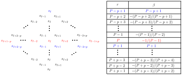
Figure 1: Values of $r$ and $\beta$ for each row of the diamond.

Let us now calculate the coefficent of $f_{\mathfrak{s}_{d}}$ under the action of $\mathbb{U}_{i}$ on $f_{\mathfrak{s}_{u}}$. The contribution to this coefficient for each $\psi_{i}$ of the middle row of the diamond is given by always choosing the first term of (5.23). This implies that the coefficient of $f_{\mathfrak{s}_{d}}$ always comes from ’going down’ and so $\alpha=1$ for all occurrences of (5.21) involved in the coefficient of $f_{\mathfrak{s}_{d}}$. The value of $\beta$, according to (5.22), therefore only depends on $r$ and the relevant residue differences, that are constant along the rows of the diamond.

The table in Figure 1 gives the values of $r$ and $\beta$ for each row of the diamond, where we write $P:=\varrho p$, for simplicity. The colors in the table correspond to the three cases in the definition of $\beta$ in (5.22), with red corresponding to the first case, blue to the second case and black to the third case. To get the coefficient of $f_{\mathfrak{s}_{d}}$ we must now multiply all the $\beta$’s of the table in Figure 1, with multiplicities given by the cardinalities of the rows of the diamond.

We first claim that the sign of this product is $+$. To show this we observe that the number of black or red $\beta$’s in the table in (5.22) is $p^{2}$ minus the number of blue $\beta$’s, that is $p^{2}-p=p(p-1)$ which is even, proving the claim.

The product of the $\beta$’s is therefore

$$\begin{split}&{\color[rgb]{0,0,1}{\frac{(P-p+1)}{1}}}\frac{(P-p+2)^{2}}{(P-p+1)^{2}}\frac{(P-p+3)^{3}}{(P-p+2)^{3}}\cdots\frac{(P-1)^{p-1}}{(P-2)^{p-1}}{\color[rgb]{1,0,0}{\frac{1}{(P-1)^{p}}}}{\color[rgb]{0,0,1}{\frac{(P+1)^{p-1}}{1}}}\cdots\frac{(P+p-3)^{3}}{(P+p-4)^{3}}\frac{(P+p-2)^{2}}{(P+p-3)^{2}}\frac{(P+p-1)}{(P+p-2)}=\\ &\\ &{\color[rgb]{0,0,1}{\frac{\cancel{(P-p+1)}}{1}}}\frac{\cancel{(P-p+2)^{2}}}{(P-p+1)^{\cancel{2}}}\frac{\cancel{(P-p+3)^{3}}}{(P-p+2)^{\cancel{3}}}\cdots\frac{\cancel{(P-1)^{p-1}}}{(P-2)^{\cancel{p-1}}}{\color[rgb]{1,0,0}{\frac{1}{(P-1)^{\cancel{p}}}}}{\color[rgb]{0,0,1}{\frac{(P+1)^{\cancel{p-1}}}{1}}}\cdots\frac{(P+p-3)^{\cancel{3}}}{\cancel{(P+p-4)^{3}}}\frac{(P+p-2)^{\cancel{2}}}{\cancel{(P+p-3)^{2}}}\frac{(P+p-1)}{\cancel{(P+p-2)}}=\\ &\\ &\frac{(P+1)}{(P-p+1)}\frac{(P+2)}{(P-p+2)}\cdots\frac{(P+p-2)}{(P-2)}\frac{(P+p-1)}{(P-1)}\end{split}$$ (6.6)

Remembering that $P=\varrho p$, we conclude from this that the coefficient of $f_{\mathfrak{s}_{d}}$ is $X$ as claimed.

In order to determine the coefficient of $f_{\mathfrak{s}_{u}}$ we use the same method as for the coefficient of $f_{\mathfrak{s}_{d}}$, with the difference that this time $\alpha$ is ’going down’ only until reaching the middle row of diamond in which it ’stand still’, and after this point, corresponding to the lower part of the diamond, $\alpha$ is ’going up’ again. Thus the table for $f_{\mathfrak{s}_{u}}$ coincides with the table in Figure 1 in the upper half of the diamond, but differs from it in the middle row and below. Using the definitions of $r$, $\alpha$ and $\beta$, we then get the following table, where we use the same color scheme as in Figure 1, and once again $P:=\varrho p$.

   (6.7)

We must calculate the product of the $\beta$’s that appear in (6.7). There is only one $\beta$ appearing with a positive sign in (6.7), namely the one in the first row, and so the sign of the product of all the $\beta$’s is $(-1)^{p^{2}-1}=1$, since $p$ is an odd prime. It is now easy to calculate the product of the $\beta$’s: indeed multiplying the $\beta$ of the first row with the $\beta$ of the last row, the $\beta$’s of the second row with the $\beta$’s of the second last row, and so on, we find that the product of the $\beta$’s is

$$\dfrac{P-p}{P}=\dfrac{\varrho p-p}{\varrho p}=\dfrac{\varrho-1}{\varrho}$$ (6.8)

which proves ${\bf b)}$

The other parts of the Theorem are proved with the same methods and are left to the reader.   $\square$

We have the following variant of Theorem 6.1 describing the right action of $\mathbb{U}_{i}$ on $\{f_{\mathfrak{s}\mathfrak{t}}\}$. Note that the formulas for the right action are the same as the formulas for the left action, except that $X$ should be replaced by $\dfrac{1}{X}$.

Theorem 6.2.

Let the notation be the same as in Theorem 6.1. Then the right action of $\mathbb{U}_{i}$ is given by

a)

$f_{\mathfrak{a}\mathfrak{s}_{d}}\mathbb{U}_{i}=\dfrac{\varrho+1}{\varrho}f_{\mathfrak{a}\mathfrak{s}_{d}}+\dfrac{X(\varrho^{2}-1)}{\varrho^{2}}f_{\mathfrak{a}\mathfrak{s}_{u}}$

b)

$f_{\mathfrak{a}\mathfrak{s}_{u}}\mathbb{U}_{i}=\dfrac{\varrho-1}{\varrho}f_{\mathfrak{a}\mathfrak{s}_{u}}+\dfrac{1}{X}f_{\mathfrak{a}\mathfrak{s}_{d}}$

Suppose that $\mathfrak{t}$ is not standard. Then $\mathbb{U}_{i}$ acts via

c)

$f_{\mathfrak{a}\mathfrak{s}}\mathbb{U}_{i}=0\,\,\,\,\,\,\,\,\,\,\mbox{ if }i,i+1\mbox{ are in the same column of }f(\mathfrak{s})$

d)

$f_{\mathfrak{a}\mathfrak{s}}\mathbb{U}_{i}=2f_{\mathfrak{a}\mathfrak{s}}\,\mbox{ if }i,i+1\mbox{ are in the same row of }f(\mathfrak{s})$

Statements similar to the one of the following Corollary, but for the original KLR-algebra ${\mathcal{R}}_{n}$ defined over a field, are already present in literature, see for example [18], [21] and [19], although the proofs in these references are different from ours, since they rely on KLR-diagrammatics.

Corollary 6.3.

Let $N_{2}$ be chosen as (4.13). Then there is an injection of Temperley-Lieb algebras

$$\iota_{KLR}:{\mathbb{TL}}_{N_{2}}^{\!{\mathbb{Z}}_{(p)}}\rightarrow{\mathbb{TL}}_{N}^{\!{\mathbb{Z}}_{(p)}},\,\,\,\mathbb{u}_{i}\mapsto\left\{f_{\mathfrak{s}\mathfrak{t}}\mapsto\mathbb{U}_{i}f_{\mathfrak{s}\mathfrak{t}}\right\}\mbox{ for }i=1,2,\ldots,N_{2}-1$$ (6.9)

Proof: We must show that the left action of the $\mathbb{U}_{i}$’s verify the Temperley-Lieb relations (2.4), (2.5) and (2.6). The quadratic relation (2.4) follows immediately from Theorem 6.1, since the $2\times 2$-matrix ${\mathbf{M}_{\mathbb{U}_{i}}}$ expressing the left action of $\mathbb{U}_{i}$ in terms of $\{f_{\mathfrak{a}\mathfrak{t}_{d}},f_{\mathfrak{a}\mathfrak{t}_{u}}\}$ has the form

$$\mathbf{M}_{\mathbb{U}_{i}}=\begin{bmatrix}\dfrac{\varrho+1}{\varrho}&X\\ \dfrac{\varrho^{2}-1}{X\varrho}&\dfrac{\varrho-1}{\varrho}\end{bmatrix}$$ (6.10)

which satisfies $\mathbf{M}_{\mathbb{U}_{i}}^{2}=\mathbf{M}_{\mathbb{U}_{i}}$.

In order to show relation (2.5), we choose $\mathfrak{s},\mathfrak{t}\in[\mathfrak{t}_{N}]\cap{\rm Std}({\rm Par}^{\leq 2}_{n})$ and show that the left action of $\mathbb{U}_{i}\mathbb{U}_{i\pm 1}\mathbb{U}_{i}$ on $f_{\mathfrak{s}\mathfrak{t}}$ is equal to the left action of $\mathbb{U}_{i}$ on $f_{\mathfrak{s}\mathfrak{t}}$. Let us focus on $\mathbb{U}_{i}\mathbb{U}_{i+1}\mathbb{U}_{i}$. We then consider the positions of $i,i+1$ and $i+2$ in $f(\mathfrak{s})$ where $f$ is as in Theorem 6.1. If $i,i+1$ and $i+2$ are in different rows of $f(\mathfrak{s})$, we have the following possibilities $\mathfrak{s}_{1},\mathfrak{s}_{2},\ldots,\mathfrak{s}_{6}$ for $f(\mathfrak{s})$.

   (6.11)

One now checks for all $j=1,2,\ldots,6$ that indeed $\mathbb{U}_{i}\mathbb{U}_{i+1}\mathbb{U}_{i}f_{\mathfrak{s}_{j}\mathfrak{t}}=\mathbb{U}_{i}f_{\mathfrak{s}_{j}\mathfrak{t}}$. For example, using $\varrho:=c_{\mathfrak{s}_{2}}(i)-c_{\mathfrak{s}_{1}}(i)$ one gets, using Theorem 6.1 repeatedly

$$\begin{split}&\mathbb{U}_{i}\mathbb{U}_{i+1}\mathbb{U}_{i}f_{\mathfrak{s}_{1}\mathfrak{t}}=\mathbb{U}_{i+1}\mathbb{U}_{i}\left(\dfrac{\varrho+1}{\varrho}f_{\mathfrak{s}_{1}\mathfrak{t}}+\dfrac{\varrho^{2}-1}{X\varrho^{2}}f_{\mathfrak{s}_{2}\mathfrak{t}}\right)=\dfrac{\varrho^{2}-1}{X\varrho^{2}}\mathbb{U}_{i+1}\mathbb{U}_{i}f_{\mathfrak{s}_{2}\mathfrak{t}}\\ &=\dfrac{\varrho^{2}-1}{X\varrho^{2}}\mathbb{U}_{i}\left(\dfrac{\varrho}{\varrho-1}f_{\mathfrak{s}_{2}\mathfrak{t}}+\dfrac{(\varrho-1)^{2}-1}{X_{1}(\varrho-1)^{2}}f_{\mathfrak{s}_{3}\mathfrak{t}}\right)=\mathbb{U}_{i}\left(\dfrac{\varrho+1}{X\varrho}f_{\mathfrak{s}_{2}\mathfrak{t}}\right)\\ &=\dfrac{\varrho+1}{X\varrho}\left(\dfrac{\varrho-1}{\varrho}f_{\mathfrak{s}_{2}\mathfrak{t}}+Xf_{\mathfrak{s}_{1}\mathfrak{t}}\right)=\dfrac{\varrho^{2}-1}{X\varrho^{2}}f_{\mathfrak{s}_{2}\mathfrak{t}}+\dfrac{\varrho+1}{\varrho}f_{\mathfrak{s}_{1}\mathfrak{t}}\end{split}$$ (6.12)

which equals $\mathbb{U}_{i}f_{\mathfrak{s}_{1}\mathfrak{t}}$. For the other $\mathfrak{s}_{j}$’s, the verification of $\mathbb{U}_{i}\mathbb{U}_{i+1}\mathbb{U}_{i}f_{\mathfrak{s}_{j}\mathfrak{t}}=\mathbb{U}_{i}f_{\mathfrak{s}_{j}\mathfrak{t}}$. is done the same way.

If two of the numbers $i,i+1$ and $i+2$ are in the same row of $f(\mathfrak{t})$ we have the following possibilities

   (6.13)

and in each case one checks that $\mathbb{U}_{i}\mathbb{U}_{i+1}\mathbb{U}_{i}$ and $\mathbb{U}_{i}$ act the same way. The verification of $\mathbb{U}_{i}\mathbb{U}_{i-1}\mathbb{U}_{i}=\mathbb{U}_{i}$ is done the same way, and finally the verification of relation (2.6) is trivial.

In order to show injectivity of $\iota_{KLR}$ one first checks that throughout the above arguments, one may always replace left actions by right actions. (This also follows from the theory in [13]).

Let now $\{C_{\mathfrak{s}\mathfrak{t}}\,|\,\mathfrak{s},\mathfrak{t}\in{\rm Std}(\lambda),\lambda\in{\rm Par}^{\leq 2}_{N_{2}}\}$ be the basis for ${\mathbb{TL}}_{N_{2}}^{\!{\mathbb{Z}}_{(p)}}$, as introduced in the paragraph before (2.23). From the formulas in Theorem 6.1 we have that $\mathfrak{u},\mathfrak{v}\in{\rm Std}(\mu)$ with $\mu\in{\rm Par}^{\leq 2}_{N_{2}}$ and $C_{\mathfrak{s}\mathfrak{t}}f_{\mathfrak{u}\mathfrak{v}}\neq 0$ implies $\mathfrak{u}\unrhd\mathfrak{t}$, and similarly, from the formulas in Theorem 6.2, we have that $f_{\mathfrak{u}\mathfrak{v}}C_{\mathfrak{s}\mathfrak{t}}\neq 0$ implies $\mathfrak{v}\unrhd\mathfrak{s}$. Moreover, we also that $C_{\mathfrak{t}^{\lambda}\mathfrak{u}}f_{\mathfrak{u}\mathfrak{v}}=\mu^{l}_{\mathfrak{u}}f_{\mathfrak{t}^{\lambda}\mathfrak{v}}$ where $\mu^{l}_{\mathfrak{u}}\neq 0$ and that $f_{\mathfrak{u}\mathfrak{v}}C_{\mathfrak{v}\mathfrak{t}^{\lambda}}=\mu^{r}_{\mathfrak{v}}f_{\mathfrak{u}\mathfrak{t}^{\lambda}}$ where $\mu^{r}_{\mathfrak{v}}\neq 0$ and where $\mathfrak{u},\mathfrak{v}$ are of shape $\lambda$.

Suppose now that $0\neq C=\sum_{\mathfrak{s},\mathfrak{t}}\lambda_{\mathfrak{s}\mathfrak{t}}C_{\mathfrak{s}\mathfrak{t}}\in{\rm ker}\,\iota_{KLR}$. Choose $(\mathfrak{s}_{0},\mathfrak{t}_{0})$ such that $\lambda_{\mathfrak{s}_{0}\mathfrak{t}_{0}}\neq 0$ and such that $(\mathfrak{s}_{0},\mathfrak{t}_{0})$ is minimal with respect to this property. Then, using $Cf_{\mathfrak{s}_{0}\mathfrak{t}_{0}}=0$ we get $0=f_{\mathfrak{t}_{0}\mathfrak{s}_{0}}Cf_{\mathfrak{s}_{0}\mathfrak{t}_{0}}=\lambda_{\mathfrak{s}_{0}\mathfrak{t}_{0}}c\,\mu^{l}_{\mathfrak{s}_{0}}\mu^{r}_{\mathfrak{t}_{0}}f_{\mathfrak{t}_{0}\mathfrak{t}_{0}}$, where $c\neq 0$, which implies $\lambda_{\mathfrak{s}_{0}\mathfrak{t}_{0}}=0$. This is however a contradiction, and so the injectivity of $\iota_{KLR}$ has been proved.

$\square$

Let $\{\textswab{L}_{1},\textswab{L}_{2},\ldots,\textswab{L}_{N_{2}}\}$ be the family of $\mathbf{JM}$-elements in ${\mathbb{TL}}_{N_{2}}^{\!{\mathbb{Z}}_{(p)}}$ given by $\textswab{L}_{i}:=\Phi(L_{i})$ where $\{L_{1},L_{2},\ldots,L_{N_{2}}\}\subseteq\mathbb{Z}_{(p)}\mathfrak{S}_{N_{2}}$ is the original family of $\mathbf{JM}$-elements in (2.26) and where $\Phi:\mathbb{Z}_{(p)}\mathfrak{S}_{N_{2}}\rightarrow{\mathbb{TL}}_{N_{2}}^{\!{\mathbb{Z}}_{(p)}}$ is the surjection from Lemma 2.4. Using the general theory in [25], we then obtain idempotents $\mathbf{E}_{\mathfrak{t}}\in{\mathbb{TL}}_{N_{2}}^{\!\mathbb{Q}}$ for $\mathfrak{t}\in{\rm Par}^{\leq 2}_{N_{2}}$ that are common eigenvectors for the $\textswab{L}_{i}$’s, via the construction in (3.12) and Corollary 3.8. On the other hand, the inclusion $\iota_{KLR}:{\mathbb{TL}}_{N_{2}}^{\!{\mathbb{Z}}_{(p)}}\rightarrow{\mathbb{TL}}_{n}^{\!{\mathbb{Z}}_{(p)}}$ from Corollary 6.3 induces an inclusion $\iota_{KLR}^{\mathbb{Q}}:{\mathbb{TL}}_{N_{2}}^{\!\mathbb{Q}}\subseteq{\mathbb{TL}_{n}^{\!\mathbb{Q}}}$ and so we may view the $\mathbf{E}_{\mathfrak{t}}$’s as idempotents in ${\mathbb{TL}_{n}^{\!\mathbb{Q}}}$ via $\iota_{KLR}^{\mathbb{Q}}$.

Our next goal is to show that, quite surprisingly, these new idempotents $\{\mathbf{E}_{\mathfrak{t}}\,|\,\mathfrak{t}\in{\rm Std}({\rm Par}^{\leq 2}_{N_{2}})$, viewed as elements in ${\mathbb{TL}_{n}^{\!\mathbb{Q}}}$, are closely related to the first idempotents $\{\mathbb{E}_{\mathfrak{t}}\,|\,\mathfrak{t}\in{\rm Std}({\rm Par}^{\leq 2}_{n})\}$ in ${\mathbb{TL}_{n}^{\!\mathbb{Q}}}$. We start with the following Lemma, which should be compared with Lemma 3.5.

Lemma 6.4.

Let $\lambda\in{\rm Std}({\rm Par}^{\leq 2}_{n})$ and suppose that $\mathfrak{t}=\mathfrak{t}_{\lambda}\in[\mathfrak{t}_{N}]\cap{\rm Std}({\rm Par}^{\leq 2}_{n})$ and that $\mathfrak{a}\in[\mathfrak{t}_{N}]\cap{\rm Std}(\lambda)$. Set $\mathfrak{s}:=f(\mathfrak{t}_{\lambda})\in{\rm Par}^{\leq 2}_{N_{2}}$ where $f$ is as in Theorem 6.1. Let $f_{\mathfrak{t}\mathfrak{a}}$ and $f_{\mathfrak{a}\mathfrak{t}}$ be as in (5.17). Then for for $i=1,2,\ldots,N_{2}$ we have that

$$\textswab{L}_{i}f_{\mathfrak{t}\mathfrak{a}}=c_{\mathfrak{s}}(i)f_{\mathfrak{t}\mathfrak{a}}\,\,\,\,\,\,\,\mbox{and}\,\,\,\,\,\,\,f_{\mathfrak{t}\mathfrak{a}}\textswab{L}_{i}=c_{\mathfrak{s}}(i)f_{\mathfrak{t}\mathfrak{a}}$$ (6.14)

Proof: Let us show the formula for the left action of $\textswab{L}_{i}$. Letting $l_{1}$ and $l_{2}$ be the column lengths of $\mathfrak{s}$ we have that

$$\mathfrak{s}=\raisebox{-0.5pt}{\includegraphics[scale={0.6}]{dib86.pdf}}\,\,$$ (6.15)

Once again, we use the recursive formula $\textswab{L}_{i+1}=(\mathbb{U}_{i}-\mathbb{1})\textswab{L}_{i}(\mathbb{U}_{i}-\mathbb{1})+\mathbb{U}_{i}-\mathbb{1}.$ Together with ${\bf c)}$ of Theorem 6.1, it reduces the proof to the case $l_{2}=1$ and $i=l_{1}+1$ where we must show that

$$\textswab{L}_{l_{1}+1}f_{\mathfrak{t}\mathfrak{t}}=f_{\mathfrak{t}\mathfrak{t}}$$ (6.16)

We do so by induction over $l_{1}$. The basis of the induction, corresponding to $l_{1}=1$, is the affirmation that $\textswab{L}_{2}f_{\mathfrak{t}\mathfrak{a}}=f_{\mathfrak{t}\mathfrak{a}}\Longleftrightarrow(\mathbb{U}_{1}-\mathbb{1})f_{\mathfrak{t}\mathfrak{a}}=f_{\mathfrak{t}\mathfrak{a}}$ which is true by ${\bf d)}$ of Theorem 6.1.

To show the inductive step $l_{1}-1\Longrightarrow l_{1}$ we write for simplicity $l:=l_{1}$, $\mathfrak{t}_{d}:=\mathfrak{t}$ and $\mathfrak{t}_{u}:=\mathfrak{t}\cdot s_{l}$ and get via ${\bf a)}$ and ${\bf b)}$ of Theorem 6.1 that

$$\begin{split}&\textswab{L}_{l+1}f_{\mathfrak{t}\mathfrak{a}}=\Big{(}\mathbb{U}_{l}-\mathbb{1})\textswab{L}_{l}(\mathbb{U}_{l}-\mathbb{1})+\mathbb{U}_{l}-\mathbb{1}\Big{)}f_{\mathfrak{t}_{d}\mathfrak{a}}=\textswab{L}_{l}(\mathbb{U}_{l}-\mathbb{1})\Big{(}\dfrac{1}{l}f_{\mathfrak{t}_{d}\mathfrak{t}}+\dfrac{l^{2}-1}{X\,l^{2}}f_{\mathfrak{t}_{u}\mathfrak{t}}\Big{)}+\Big{(}\dfrac{1}{l}f_{\mathfrak{t}_{d}\mathfrak{a}}+\dfrac{l^{2}-1}{X\,l^{2}}f_{\mathfrak{t}_{u}\mathfrak{a}}\Big{)}\\ &=(\mathbb{U}_{l}-\mathbb{1})\Big{(}\dfrac{1-l}{l}f_{\mathfrak{t}_{d}\mathfrak{a}}+\dfrac{l^{2}-1}{X\,l^{2}}f_{\mathfrak{t}_{u}\mathfrak{a}}\Big{)}+\Big{(}\dfrac{1}{l}f_{\mathfrak{t}_{d}\mathfrak{a}}+\dfrac{l^{2}-1}{X\,l^{2}}f_{\mathfrak{t}_{u}\mathfrak{a}}\Big{)}=\mathbb{U}_{l}\Big{(}\dfrac{1-l}{l}f_{\mathfrak{t}_{d}\mathfrak{a}}+\dfrac{l^{2}-1}{X\,l^{2}}f_{\mathfrak{t}_{u}\mathfrak{a}}\Big{)}+f_{\mathfrak{t}_{d}\mathfrak{a}}\\ &=\dfrac{1-l}{l}\mathbb{U}_{l}\Big{(}f_{\mathfrak{t}_{d}\mathfrak{a}}-\dfrac{l+1}{X\,l}f_{\mathfrak{t}_{u}\mathfrak{a}}\Big{)}+f_{\mathfrak{t}_{d}}=f_{\mathfrak{t}_{d}\mathfrak{a}}=f_{\mathfrak{t}\mathfrak{a}}\end{split}$$ (6.17)

The proof of the formula for the right action is done the same way.

$\square$

The previous Lemma is the basis step for the inductive proof of the following Theorem which should be compared with Theorem 3.7.

Theorem 6.5.

Suppose that $\mathfrak{t},\mathfrak{a}\in[\mathfrak{t}_{N}]\cap{\rm Std}({\rm Par}^{\leq 2}_{n})$. Set $\mathfrak{s}:=f(\mathfrak{t})\in{\rm Par}^{\leq 2}_{N_{2}}$ where $f$ is as in Theorem 6.1. Then for $i=1,2,\ldots,N_{2}$ we have that

$$\textswab{L}_{i}f_{\mathfrak{t}\mathfrak{a}}=c_{\mathfrak{s}}(i)f_{\mathfrak{t}\mathfrak{a}}\,\,\,\,\,\,\,\mbox{and}\,\,\,\,\,\,\,f_{\mathfrak{a}\mathfrak{t}}\textswab{L}_{i}=c_{\mathfrak{s}}(i)f_{\mathfrak{a}\mathfrak{t}}$$ (6.18)

Proof: As already indicated, the proof is by upwards induction over the dominance order in ${\rm Std}(\lambda)$, with Lemma 6.4 corresponding to the induction basis. The induction step is carried out the same way as the induction step in the proof of Theorem 3.7, with Theorem 6.1 replacing Theorem 3.4. The extra factors $X$ or $1/X$ in the equations corresponding to (3.35)–(3.38) do not affect the conclusion.   $\square$

We have two Corollaries to Theorem 6.5.

Corollary 6.6.

Let $\mathfrak{t}$ and $\mathfrak{s}$ be as in Theorem 6.5 and let $\mathbb{E}_{\mathfrak{t}}\in{\mathbb{TL}_{n}^{\!\mathbb{Q}}}$ be the idempotent from Corollary 3.8. Then we have

$$\textswab{L}_{i}\mathbb{E}_{\mathfrak{t}}=\mathbb{E}_{\mathfrak{t}}\textswab{L}_{i}=c_{\mathfrak{s}}(i)\mathbb{E}_{\mathfrak{t}}\,\mbox{ for }i=1,2,\ldots,N_{2}$$ (6.19)

Proof: This follows directly from Theorem 6.5 together with the construction of $\mathbb{E}_{\mathfrak{t}}$ in (3.12) and Corollary 3.8.   $\square$

Corollary 6.7.

Suppose that $\mathfrak{t}\in[\mathfrak{t}_{N}]\cap{\rm Std}({\rm Par}^{\leq 2}_{n})$ and that $\mathfrak{s}\in{\rm Par}^{\leq 2}_{N_{2}}$ where $N_{2}$ is as in Lemma 4.14. Let $\iota_{KLR}^{\mathbb{Q}}:{\mathbb{TL}}_{N_{2}}^{\!\mathbb{Q}}\subseteq{\mathbb{TL}_{n}^{\!\mathbb{Q}}}$ be the inclusion given by Corollary 6.3. Then we have

$$\iota_{KLR}^{\mathbb{Q}}\big{(}\mathbf{E}_{\mathfrak{s}}\big{)}\cdot\mathbb{E}_{\mathfrak{t}}=\mathbb{E}_{\mathfrak{t}}\,\cdot\iota_{KLR}^{\mathbb{Q}}\big{(}\mathbf{E}_{\mathfrak{s}}\big{)}=\begin{cases}\mathbb{E}_{\mathfrak{t}}&\mbox{ if }f(\mathfrak{t})=\mathfrak{s}\\ 0&\text{ if }f(\mathfrak{t})\neq\mathfrak{s}\end{cases}$$ (6.20)

Proof: Suppose first that $f(\mathfrak{t})=\mathfrak{s}$. Using (3.2) and Corollary 6.6 we then get

$$\iota_{KLR}^{\mathbb{Q}}\big{(}\mathbf{E}_{\mathfrak{s}}\big{)}\cdot\mathbb{E}_{\mathfrak{t}}=\left(\prod_{c\in{\cal C}}\,\,\prod_{\begin{subarray}{c}i=1,\ldots,N_{2}\\ c\neq c_{\mathfrak{s}}(i)\end{subarray}}\dfrac{\textswab{L}_{i}-c}{c_{\mathfrak{s}}(i)-c}\right)\mathbb{E}_{\mathfrak{t}}=\left(\prod_{c\in{\cal C}}\,\,\prod_{\begin{subarray}{c}i=1,\ldots,N_{2}\\ c\neq c_{\mathfrak{s}}(i)\end{subarray}}\dfrac{c_{\mathfrak{s}}(i)-c}{c_{\mathfrak{s}}(i)-c}\right)\mathbb{E}_{\mathfrak{t}}=\mathbb{E}_{\mathfrak{t}}$$ (6.21)

as claimed. Suppose next that $f(\mathfrak{t})\neq\mathfrak{s}$. Then there is $i\in\{1,2,\ldots,N_{2}\}$ such that $c_{f(\mathfrak{t})}(i)\neq c_{\mathfrak{s}}(i)$, since the separability condition (3.1) is fulfilled, and so $\iota_{KLR}^{\mathbb{Q}}\big{(}\mathbf{E}_{\mathfrak{s}}\big{)}$ has $\big{(}\textswab{L}_{i}-c_{f(\mathfrak{t})}(i)\big{)}$ as a factor. But by Corollary 6.6 we have $\big{(}\textswab{L}_{i}-c_{f(\mathfrak{t})}(i)\big{)}E_{\mathfrak{t}}=0$ which implies $\iota_{KLR}^{\mathbb{Q}}\big{(}\mathbf{E}_{\mathfrak{s}}\big{)}E_{\mathfrak{t}}=0$. The formula for the right action is proved the same way.

$\square$

In the rest of the article we shall show how ${}^{p}\!{\mathbf{JW}_{\!n}}$ fits into the picture. Recall from (4.3) the expansion of $n+1$ in base $p$

$$n+1=a_{k}p^{k}+a_{k-1}p^{k-1}+\ldots+a_{1}p+a_{0}$$ (6.22)

From (4.13) we have $n=N=N_{1}+(p-1)$ and $N_{1}=pN_{2}+R$ and so we get

$$R=a_{0}\,\,\mbox{ and }N_{2}+1=a_{k}p^{k-1}+a_{k-1}p^{k-2}+\ldots+a_{1}$$ (6.23)

Repeating this process we find that $N,N_{1},N_{2}$ and $R$ belong to sequences of natural numbers $N^{i},N_{1}^{i},N_{2}^{i}$ and $R^{i}$ where $N:=N^{0},N_{1}=N_{1}^{0},N_{2}=N_{2}^{0}$ and $R=R^{0}$ and where

$$N^{i}=N_{1}^{i}+(p-1),\,\,\,N^{i}_{1}=pN^{i}_{2}+R^{i},\,\,\,N^{i+1}=N_{2}^{i}\,\mbox{ for }i=0,1,\ldots,k-1$$ (6.24)

In fact we have

$$R^{i}=a_{i}\,\,\mbox{ and }N_{2}^{i}+1=a_{k}p^{k-i-1}+a_{k-1}p^{k-i-2}+\ldots+a_{i+1}$$ (6.25)

Using Corollary 6.9 we then get a chain of injections

$${\mathbb{TL}}_{N^{k-1}_{2}}^{\!{\mathbb{Z}}_{(p)}}\subseteq{\mathbb{TL}}_{N^{k-2}_{2}}^{\!{\mathbb{Z}}_{(p)}}\subseteq\cdots\subseteq{\mathbb{TL}}_{N_{2}^{0}}^{\!{\mathbb{Z}}_{(p)}}={\mathbb{TL}}_{N}^{\!{\mathbb{Z}}_{(p)}}={\mathbb{TL}}_{n}^{\!{\mathbb{Z}}_{(p)}}$$ (6.26)

Let $\mathbf{E}_{[\mathfrak{t}_{N^{i}_{2}}]}$ be the class idempotent for ${\mathbb{TL}}_{N_{2}^{i}}^{\!{\mathbb{Z}}_{(p)}}$. We may view it as an idempotent of ${\mathbb{TL}}_{n}^{\!{\mathbb{Z}}_{(p)}}$ via the chain in (6.26).

We can now prove the following main Theorem. It establishes the promised connection between the $p$-Jones-Wenzl idempotents and KLR-theory for the Temperley-Lieb algebra, via the seminormal form approach to KLR-theory.

Theorem 6.8.

In the above setting we have

$$^{p}\!{\mathbf{JW}_{\!n}}=\prod_{i=0}^{k-1}\mathbf{E}_{[\mathfrak{t}_{N^{i}_{2}}]}$$ (6.27)

Proof: $\mathbf{E}_{[\mathfrak{t}_{N^{0}_{2}}]}=\mathbf{E}_{[\mathfrak{t}_{n}]}=\sum_{\mathfrak{t}\in[\mathfrak{t}_{n}]}\mathbb{E}_{\mathfrak{t}}$ is the class idempotent for ${\mathbb{TL}_{n}^{\!{\mathbb{Z}}_{(p)}}}$ and so we get from Corollary 6.7 that the right hand side RHS of (6.27) has the form

$${\rm RHS}=\sum_{\mathfrak{t}\in\mathcal{A}_{n}}\mathbb{E}_{\mathfrak{t}}$$ (6.28)

for $\mathcal{A}$ a subset of $[\mathfrak{t}_{n}]$. We must show that $\mathcal{A}_{n}={\mathcal{I}}_{n}$, where ${\mathcal{I}}_{n}$ is as in (4.4). Given $\mathfrak{t}\in\mathcal{A}_{n}$ we must therefore show that $\mathfrak{t}$ is given by blocks $D_{1},M_{1},D_{2},M_{2},\ldots,D_{k},M_{k}$ of consecutive numbers, of the cardinalities specified in the paragraphs following (4.4).

Let us first focus on the numbers $\{1,2,\ldots,(a_{k}p^{k}-1)\}$ in $\mathfrak{t}$. We must show that they all appear in the first column of $\mathfrak{t}$. But as already observed in the preceding sections, since $\mathbf{E}_{[\mathfrak{t}_{N^{0}_{2}}]}$ is a factor of RHS certainly the numbers $\{1,2,\ldots,p-1\}$ all appear in the first column of $\mathfrak{t}$.

We then consider the numbers $\{p,p+1,\ldots(a_{k}p^{k}-1)\}$ grouped in blocks of cardinality $p$. But $\mathbf{E}_{[\mathfrak{t}_{N^{1}_{2}}]}$ is a factor of RHS, from which we deduce that the first $p-1$ of these blocks also appear in the first column of $\mathfrak{t}$. We have $(p-1)+(p-1)p=p^{2}-1$ and so we have shown that the numbers $\{1,2,\ldots,p^{2}-1\}$ appear in the first column of $\mathfrak{t}$. We next consider blocks of cardinality $p^{2}$ and use the factor factor $\mathbf{E}_{[\mathfrak{t}_{N^{2}_{2}}]}$ to show that in fact the numbers $\{1,2,\ldots,p^{3}-1\}$ all appear in the first column of $\mathfrak{t}$. Repeating this argument, we finally get that the numbers $\{1,2,\ldots,(a_{k}p^{k}-1)\}$ all appear in the first column of $\mathfrak{t}$, as claimed.

But using that $\mathbf{E}_{[\mathfrak{t}_{N^{k-2}_{2}}]}$ is a factor of RHS, we now get that the $a_{k-1}p^{k-1}$ numbers following $\{1,2,\ldots,(a_{k}p^{k}-1)\}$ all appear either in first or in the second column of $\mathfrak{t}$. Repeating this last argument recursively, we finally find that $\mathfrak{t}\in\mathcal{A}_{n}$, as claimed. The Theorem is proved.

$\square$

References

[1] J. Brundan, A. Kleshchev,
Blocks of cyclotomic Hecke algebras and Khovanov-Lauda algebras, Invent. Math. 178, (2009), 451-484.
[2] C. Bowman, A. Cox, A. Hazi, Path isomorphisms between quiver Hecke and diagrammatic Bott-Samelson endomorphism algebras, arXiv:2005.02825.
[3]
G. Burrull, N. Libedinsky, P. Sentinelli, p-Jones-Wenzl idempotents,
Adv. Math. 352, (2019), 246-264.
[4] B. Elias, N. Libedinsky, Indecomposable Soergel bimodules for universal Coxeter groups.
With an appendix by Ben Webster, Trans. Am. Math. Soc.
369(6) (2017), 3883-3910.
[5]
M. Ehrig, C. Stroppel, Koszul gradings on Brauer algebras,
Int. Math. Res. Not. 2016 (13), (2016), 3970-4011.
[6] K. Erdmann, A. Henke, On Ringel duality for Schur algebras, Math. Proc. Cambridge Philos. Soc. 132, (2002), 97–116.
[7] J. J. Graham, G. I. Lehrer,
Cellular algebras, Inventiones Mathematicae 123, (1996), 1-34.
[8] J. J. Graham, G. I. Lehrer,
The representation theory of affine Temperley-Lieb algebras,
Enseign. Math., II. Sér. 44(3-4), (1998), 173-218.
[9] F. M. Goodman, H. Wenzl,
The Temperley-Lieb Algebra at roots of unity,
Pacific Journal of Mathematics 161(2), (1993), 307-334.
[10] F. M. Goodman, H. Wenzl,
Ideals in the Temperley-Lieb category, appendix to: A mathematical
model with a possible Chern-Simons phase by M. Freedman, Comm. Math. Phys. 234, (2003),
129–183.
[11]
A. Hazi, P. Martin, A. Parker, Indecomposable tilting modules for the blob algebra,
Journal of Algebra 568, (2021), 273-313.
[12] J. Hu, A. Mathas, Graded cellular bases for the cyclotomic Khovanov-Lauda-Rouquier
algebras of type , Adv. Math., 225, (2010), 598-642.
[13]
J. Hu, A. Mathas,
Seminormal forms and cyclotomic quiver Hecke algebras of type A,
Math. Ann. 364(3-4), (2016), 1189-1254.
[14] M. Härterich,
Murphy bases of generalized Temperley-Lieb algebras,
Arch. Math. 72(5), (1999), 337-345.
[15] J. E. Humphreys, Reflection groups and Coxeter groups, volume 29 of Cambridge Studies in
Advanced Mathematics. Cambridge University Press, Cambridge, (1990).
[16] V.F.R. Jones, Index for subfactors, Invent. Math. 72(1), (1983), 1–25.
[17] M. Khovanov, A. Lauda, A diagrammatic approach to categorification of quantum groups I, Represent. Theory 13, (2009), 309-347.
[18]
A. Kleshchev, A. Mathas, A. Ram, Universal graded Specht modules for cyclotomic Hecke algebras,
Proc. Lond. Math. Soc. (3) 105(6), (2012), 1245-1289.
[19] N. Libedinsky, D. Plaza, Blob algebra approach to modular representation theory,
Proc. of the London Math. Soc. (121)(3), (2020), 656-701.
[20] D. Lobos, On Generalized blob algebras: Vertical idempotent truncations and Gelfand-Tsetlin subalgebras, arXiv:2203.15139.
[21] D. Lobos, D. Plaza, S. Ryom-Hansen,
The nil-blob algebra: an incarnation of type
Soergel calculus and of the truncated blob algebra,
Journal Algebra 570, (2021), 297-365.
[22] D. Lobos, S. Ryom-Hansen,
Graded cellular basis and Jucys-Murphy elements
for generalized blob algebras,
Journal of Pure and Applied Algebra,
224(7), (2020), 106277, 1-40.
[23] P. Martin,
Potts models and related problems in statistical mechanics,
Series on Advances in Statistical Mechanics, 5. Singapore etc.: World Scientific. xiii, 344 pages,
(1991).
[24] A. Mathas,
Hecke algebras and Schur algebras of the symmetric group,
Univ. Lecture Notes, 15, A.M.S., Providence, R.I., (1999).
[25] A. Mathas, Seminormal forms and Gram determinants for cellular algebras, J.
Reine Angew. Math., 619, (2008), 141-173. With an appendix by M. Soriano.
[26] G. E. Murphy, A new construction of Young’s seminormal representation of the symmetric groups,
J. of Algebra 69, (1981), 287-297.
[27] G. E. Murphy, The idempotents of the symmetric group and
Nakayama’s conjecture, J. of Algebra 81, (1983), 258-265.
[28] G. E. Murphy, The Representations of Hecke Algebras of type
, J. of Algebra 173, (1995), 97-121.
[29] G. E. Murphy, On the Representation Theory of the Symmetric Groups and associated Hecke Algebras,
J. of Algebra 152, (1992),, 492-513.
[30] K. Ormeño, Elementos de Jucys-Murphy en el álgebra de Temperley-Lieb,
Tesis de magister, Universidad de Talca.
[31]
D. Plaza, S. Ryom-Hansen, Graded cellular bases for Temperley-Lieb algebras of type A and B,
Journal of Algebraic Combinatorics, 40(1), (2014), 137-177.
[32]
R. Rouquier, 2-Kac-Moody algebras, arXiv:0812.5023.
[33] S. Ryom-Hansen, Jucys-Murphy elements for Soergel bimodules, Journal of Algebra, 551, (2020), 154-190.
[34]
M. Stuart, R. A. Spencer,
-Jones-Wenzl idempotents,
J. Algebra 603, (2022), 41-60.
[35]
L. Sutton, D. Tubbenhauer, P. Wedrich, J. Zhu,
tilting modules in the mixed case,
arXiv:2105.07724.
[36]
D. Tubbenhauer, P. Wedrich,
Quivers for
tilting modules,
Represent. Theory 25, (2021), 440-480.
[37]
D. Tubbenhauer, P. Wedrich,
The center of
tilting modules,
Glasg. Math. J. 64(1), (2022), 165-184.
[38] H. Wenzl, On sequences of projections, C. R. Math. Rep. Acad. Sci. Can. 9 1,
(1987), 5–9.