Distributed exact quantum algorithms for Bernstein-Vazirani and search problems

Abstract

Distributed quantum computation has gained extensive attention since small-qubit quantum computers seem to be built more practically in the noisy intermediate-scale quantum (NISQ) era. In this paper, we give a distributed Bernstein-Vazirani algorithm (DBVA) with $t$ computing nodes, and a distributed exact Grover’s algorithm (DEGA) that solve the search problem with only one target item in the unordered databases. Though the designing techniques are simple in the light of BV algorithm, Grover’s algorithm, the improved Grover’s algorithm by Long, and the distributed Grover’s algorithm by Qiu et al, in comparison to BV algorithm, the circuit depth of DBVA is not greater than $2^{\text{max}(n_{0},n_{1},\cdots,n_{t-1})}+3$ instead of $2^{n}+3$, and the circuit depth of DEGA is $8(n~{}\text{mod}~{}2)+9$, which is less than the circuit depth of Grover’s algorithm, $1+8\left\lfloor\frac{\pi}{4}\sqrt{2^{n}}\right\rfloor$. In particular, we provide situations of our DBVA and DEGA on MindQuantum (a quantum software) to validate the correctness and practicability of our methods. By simulating the algorithms running in the depolarized channel, it further illustrates that distributed quantum algorithm has superiority of resisting noise.

1 Introduction

Quantum computation, a novel computing model, utilizes quantum information units to perform computation depending on the laws of quantum mechanics. It has attracted considerable attention in the past couple of decades since Benioff [1, 2] proposed the concept of the quantum Turing machine in 1980. Subsequently, a great number of remarkable and valuable quantum algorithms have been presented, such as Deutsch’s algorithm [3], Deutsch-Jozsa (DJ) algorithm [4], Bernstein-Vazirani (BV) algorithm [5], Simon’s algorithm [6], Shor’s algorithm [7], Grover’s algorithm [8], HHL algorithm [9] and so on. For some specific problems, quantum algorithms have the potential to offer essential advantages over classical algorithms.

Bernstein-Vazirani (BV) algorithm [5] was proposed after DJ algorithm. It proves that quantum algorithms are capable of not only determining properties of Boolean functions [10, 11, 12], but also determining the functions themselves. For BV problem, it aims to find the hidden string $s\in\{0,1\}^{n}$ satisfying the function $f_{s}(x)=\langle s\cdot x\rangle=\left(\sum_{i=0}^{n-1}s_{i}\cdot x_{i}\right)~{}\text{mod}~{}2:\{0,1\}^{n}\rightarrow\{0,1\}$. Suppose we have a black box (Oracle) that can return $f_{s}(x_{0})$ for an input $x_{0}$. In order to solve the BV problem, the classical algorithm will have to query Oracle $n$ times, while the BV algorithm will just need to query once. In 2017, Nagata et al. [13] presented a generalized Bernstein-Vazirani algorithm.

Grover’s algorithm [8] was proposed by Grover in 1996, which is a quantum search algorithm that solves the search problem in an unordered databases with $2^{n}$ elements. Specifically, let Boolean function $f:\{0,1\}^{n}\rightarrow\{0,1\}$. For the $m$ targets search problem, it aims to find out one target string $x_{i}\in\{0,1\}^{n}$ satisfying $f(x_{i})=1$, where $i\in\{0,1,\cdots,m-1\}$. Suppose we have a black box (Oracle) that can recognize the inputs, which means it will return $f(x)=1$ when $x$ is a target string, and output $f(x)=0$ otherwise. The classical algorithms have to query Oracle $\mathcal{O}(2^{n}/m)$ times, while Grover’s algorithm just need to query $\mathcal{O}(\sqrt{2^{n}/m})$ times to figure out the target string with high probability, which has square acceleration compared with the classical algorithms.

Grover’s algorithm has been widely used in the minimum search problem [14], string matching problem [15], quantum dynamic programming [16] and computational geometry problem [17], etc. Subsequently, a generalization of Grover’s algorithm known as the quantum amplitude amplification and estimation algorithms [18] were presented.

However, Grover’s algorithm is unable to search for the target state accurately, except in the case of looking for one data in an unordered database with a size of four [19]. In 2001, Long [20] improved Grover’s algorithm, which acquires the goal state exactly.

Currently, quantum computation is entering the noisy intermediate-scale quantum (NISQ) era [21]. During this period, a great deal of theoretical and experimental work has been devoted to the development of quantum devices. Studies on small-scale quantum computers based on ions [22], photons [23], superconduction [24], and other quantum systems [25, 26] have been extensively conducted. It may contain tens to thousands of qubits with a gate error rate of less than $10^{-3}$ [27]. Currently, small-qubit quantum computers seem to be built more practically, compared to large-scale universal quantum computers. Hence, researchers are considering how several small-scale devices might collaborate to accomplish a task on a large scale.

Distributed quantum computation, a research field in computer science, combines distributed computing and quantum computation. It aims to divide a large problem into many small parts and then distribute them across multiple quantum computers for processing. In this way, each component needs fewer qubits and has a shallower quantum circuit.

There has been great interest in distributed quantum algorithms [28, 29, 30, 31]. Avron et al. [32] proposed a distributed method for constructing Oracles. Qiu et al. [33] proposed two distributed Grover’s algorithms (parallel and serial) and these algorithms require fewer qubits and have shallower depth of circuits. Also, the distributed algorithms by Qiu et al. [33] can solve the search problem with multiple targets. They [33] divided a Boolean function $f$ into $2^{k}$ subfunctions, where $2^{k}$ represents the number of computing nodes. Theyr determine the number of solutions in each subfunction by using the quantum counting algorithm, and then ran $(n-k)$-qubit Grover’s algorithm for each subfunction. Particularly, Qiu et al. [33] proposed an efficient algorithm of constructing quantum circuits for realizing the Oracle corresponding to any Boolean function with conjunctive normal form (CNF).

Tan, Xiao, and Qiu et al. [34] presented an interesting and novel distributed Simon’s algorithm. Recently, Xiao and Qiu et al. [35] proposed a distributed Shor’s algorithm, which can separately estimate patrial bits of $s/r$ for some $s\in\{0,1,\cdots,r-1\}$ by two quantum computers during solving order-finding.

In this paper, we give a distributed Bernstein-Vazirani algorithm (DBVA) with $t$ computing nodes. After that, we present a distributed exact Grover’s algorithm (DEGA) for the case of only one target item in the unordered databases. DBVA and DEGA are distributed exact quantum algorithm. In comparison to the BV algorithm, the circuit depth of DBVA is not greater than $2^{\text{max}(n_{0},n_{1},\cdots,n_{t-1})}+3$ instead of $2^{n}+3$. The circuit depth of DEGA is $8(n~{}\text{mod}~{}2)+9$, which is less than the circuit depths of the original Grover’s algorithm, $1+8\left\lfloor\frac{\pi}{4}\sqrt{2^{n}}\right\rfloor$.

MindQuantum (a quantum software) [36] is a general software library supporting the development of applications for quantum computation. In this paper, we provide particular situations of our DBVA and DEGA on MindQuantum to validate the correctness and practicability of our methods. At the first, we explicate the concrete circuits of a 6-qubit DBVA on MindQuantum as an example, which shows how to decompose the original 6-qubit BV problem into two 3-qubit and three 2-qubit tasks. In the next part, we explicate the specific steps of implement $n$-qubit DEGA, where $n\in\{2,3,4,5\}$. In the end, by simulating the 6-qubit DBVA and 5-qubit DEGA running in the depolarized channel, it further illustrates that distributed quantum algorithm has superiority of resisting noise.

The rest of the paper is organized as follows. We will review BV algorithm and Grover’s algorithm in Section 2 and mainly describe our DBVA and DEGA in Section 3 and Section 4. Next, the analysis of our algorithms will be presented in Section 5. After that, we provide particular situations of our DBVA and DEGA on MindQuantum in Section 6. Finally, a brief conclusion is given in Section 7.

2 Preliminaries

In this section, we will review BV algorithm [5], Grover’s algorithm [8], and the algorithm by Long [20].

2.1 Bernstein-Vazirani problem [5]

Let Boolean function $f:\{0,1\}^{n}\rightarrow\{0,1\}$. Consider a function

$$f_{s}(x)=\langle s\cdot x\rangle=\left(\sum_{i=0}^{n-1}s_{i}\cdot x_{i}\right)~{}\text{mod}~{}2,$$ (1)

where $x\in\{0,1\}^{n}$. Suppose we have an Oracle ($O_{f_{s}(x)}:|x\rangle\rightarrow(-1)^{f_{s}(x)}|x\rangle$) that can return $f_{s}(x_{0})$ for an input $x_{0}\in\{0,1\}^{n}$. For BV problem, it aims to identify the hidden string $s\in\{0,1\}^{n}$.

For BV algorithm, it will just need to query Oracle once (see Figure 1).

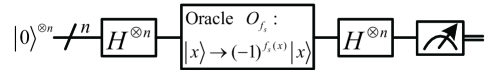
Figure 1: Quantum circuit of the BV algorithm.

The evolution of the quantum state in BV algorithm is shown below:

$$|0\rangle^{\otimes n} \stackrel{{\scriptstyle H^{\otimes n}}}{{\longrightarrow}} \frac{1}{\sqrt{2^{n}}}\sum_{x\in\{0,1\}^{n}}|x\rangle$$ (2)

$$\stackrel{{\scriptstyle O_{f_{s}(x)}}}{{\longrightarrow}} \frac{1}{\sqrt{2^{n}}}\sum_{x\in\{0,1\}^{n}}(-1)^{f_{s}(x)}|x\rangle=\frac{1}{\sqrt{2^{n}}}\sum_{x\in\{0,1\}^{n}}(-1)^{\langle s\cdot x\rangle}|x\rangle$$

$$= \frac{1}{\sqrt{2^{n}}}\sum_{x_{0}x_{1}\cdots x_{n-1}\in\{0,1\}^{n}}(-1)^{\left(\sum_{i=0}^{n-1}s_{i}\cdot x_{i}\right)~{}\text{mod}~{}2}|x_{0}x_{1}\cdots x_{n-1}\rangle$$

$$\stackrel{{\scriptstyle H^{\otimes n}}}{{\longrightarrow}} |s_{0}s_{1}s_{2}\cdots s_{n-1}\rangle=|s\rangle.$$

2.2 Grover’s algorithm [8]

Suppose that the search task is carried out in an unordered set (or database) with $2^{n}$ elements. We establish a one-to-one correspondence between the elements in the database and the indexes (integers from 0 to $2^{n}-1$). We focus on searching the indexes of these elements.

Let Boolean function $f:\{0,1\}^{n}\rightarrow\{0,1\}$. Define a function for the search problem as follows:

$$f(x)=\begin{cases}1,x=\tau,\\ 0,x\neq\tau,\end{cases}$$ (3)

where $x\in\{0,1\}^{n}$ and $\tau$ is the target index. In a quantum system, indexes are represented by quantum states $|0\rangle,|1\rangle,\cdots,|2^{n}-1\rangle$ (or $|00\cdots 0\rangle,|00\cdots 1\rangle,\cdots,|11\cdots 1\rangle$).

Without losing of generality, we consider a search problem that includes only one target item in the unordered databases throughout this paper. Suppose we have a black box (Oracle $U_{f(x)}:|x\rangle\rightarrow(-1)^{f(x)}|x\rangle$, where $x\in\{0,1\}^{n}$) that can recognize the inputs. The purpose of Grover’s algorithm is to find out $|\tau\rangle$ with high probability.

Here, we briefly review Grover’s algorithm in Algorithm 2.2. The whole quantum circuit is shown in Figure 2.

  Algorithm 1 Grover’s Algorithm (includes only one target).

 

  Input: (1) The number of qubits $n$; (2) A function $f(x)$, where $f(x)=0$ for all $x\in\{0,1\}^{n}$ except $\tau$, for which $f(\tau)=1$.

  Initialization: An Oracle $U_{f(x)}:|x\rangle\rightarrow(-1)^{f(x)}|x\rangle$, where $x\in\{0,1\}^{n}$.

  Output: The string $\tau\in\{0,1\}^{n}$ such that $f(\tau)=1$ with great probability.

  Procedure:

  Step 1. Initialize $n$ qubits $|0\rangle^{\otimes n}$.

  Step 2. Apply $n$ Hadamard gates $H^{\otimes n}$.

  Step 3. Grover operator $G=-H^{\otimes n}U_{0}H^{\otimes n}U_{f(x)}$ is executed with $\left\lfloor\frac{\pi}{4}\sqrt{2^{n}}\right\rfloor$ times, where $U_{0}=I_{n}-2(|0\rangle\langle 0|)^{\otimes n}$ and $U_{f(x)}=I_{n}-2|\tau\rangle\langle\tau|$.

  Step 4. Measure each qubit in the basis $\{|0\rangle,|1\rangle\}$.

 

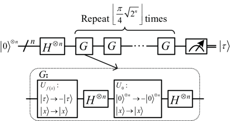
Figure 2: Quantum circuit of Grover’s algorithm.

2.3 The algorithm by Long [20]

In 2001, Long improved Grover’s algorithm, which will acquire the goal state with a probability of $100\%$. Its main idea is to extend Grover operator $G$ to another operator $L$.

Here, we briefly review this algorithm in Algorithm 2.3. The whole quantum circuit is shown in Figure 3.

  Algorithm 2 The algorithm by Long (includes only one target).

 

  Input: (1) The number of qubits $n$; (2) A function $f(x)$, where $f(x)=0$ for all $x\in\{0,1\}^{n}$ except $\tau$, for which $f(\tau)=1$.

  Initialization: An Oracle $R_{f(x)}:|x\rangle\rightarrow e^{i\phi\cdot f(x)}|x\rangle$, where $x\in\{0,1\}^{n}$, $\phi=2\arcsin\left(\sin\left(\frac{\pi}{4J+6}\right)/\sin\theta\right)$, $J=\lfloor(\pi/2-\theta)/(2\theta)\rfloor$, and $\theta=\arcsin{\sqrt{1/2^{n}}}$.

  Output: The string $\tau\in\{0,1\}^{n}$ such that $f(\tau)=1$ with a probability of $100\%$.

  Procedure:

  Step 1. Initialize $n$ qubits $|0\rangle^{\otimes n}$.

  Step 2. Apply $n$ Hadamard gates $H^{\otimes n}$.

  Step 3. Operator $L=-H^{\otimes n}R_{0}H^{\otimes n}R_{f(x)}$ is executed with $J+1$ times, where $R_{0}=I_{n}+(e^{i\phi}-1)(|0\rangle\langle 0|)^{\otimes n}$ and $R_{f(x)}=I_{n}+(e^{i\phi}-1)|\tau\rangle\langle\tau|$.

  Step 4. Measure each qubit in the basis $\{|0\rangle,|1\rangle\}$.

 

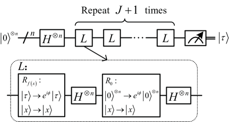
Figure 3: Quantum circuit of the algorithm by Long.

3 Distributed Bernstein-Vazirani algorithm

In this section, we mainly describe our distributed Bernstein-Vazirani algorithm (DBVA) with $t$ computing nodes.

3.1 Subfunctions

As mentioned in [32], an $n$-qubit Boolean function $f:\{0,1\}^{n}\rightarrow\{0,1\}$ can be split into two subfunctions $f_{\text{even}/\text{odd}}:\{0,1\}^{n-1}\rightarrow\{0,1\}$,

$$f_{\text{even}}(x) = f(x_{0}x_{1}\cdots x_{i-1}0x_{i+1}\cdots x_{n-2}x_{n-1}),$$ (4)

$$f_{\text{odd}}(x) = f(x_{0}x_{1}\cdots x_{i-1}1x_{i+1}\cdots x_{n-2}x_{n-1}),$$ (5)

where $x=x_{0}x_{1}\cdots x_{i-1}x_{i+1}\cdots x_{n-2}x_{n-1}\in\{0,1\}^{n-1}$.

Furthermore, if we choose last $k\in\{1,2,\cdots,n-1\}$ bits to divide $f$, we can divide the original function into $2^{k}$ subfunctions $f_{p}:\{0,1\}^{n-k}\rightarrow\{0,1\}$:

$$f_{p}(x) = f(\underbrace{x_{0}x_{1}\cdots x_{n-k-1}}_{n-k}\underbrace{y_{p_{0}}y_{p_{1}}\cdots y_{p_{k-1}}}_{k}),$$ (6)

where $k\in\{1,2,\cdots,n-1\}$, $x=x_{0}x_{1}\cdots x_{n-k-1}\in\{0,1\}^{n-k}$, and $y_{p_{0}}y_{p_{1}}\cdots y_{p_{k-1}}\in\{0,1\}^{k}$ is the binary representation of $p\in\{0,1,\cdots,2^{k}-1\}$.

More generally, $y_{p_{0}}y_{p_{1}}\cdots y_{p_{k-1}}$ can be at any $k$ positions in $x$ of the original function $f$. For instance, we can also obtain another $2^{k}$ subfunctions $f_{q}:\{0,1\}^{n-k}\rightarrow\{0,1\}$:

$$f_{q}(x) = f(\underbrace{y_{q_{0}}y_{q_{1}}\cdots y_{q_{k-1}}}_{k}\underbrace{x_{k}x_{k+1}\cdots x_{n-1}}_{n-k}),$$ (7)

where $k\in\{1,2,\cdots,n-1\}$, $x=x_{k}x_{k+1}\cdots x_{n-1}\in\{0,1\}^{n-k}$, and $y_{q_{0}}y_{q_{1}}\cdots y_{q_{k-1}}\in\{0,1\}^{k}$ is the binary representation of $q\in\{0,1,\cdots,2^{k}-1\}$.

Next, we must declare our partition strategy for the original function $f_{s}(x)$ before providing our DBVA.

Suppose that the hidden string $s\in\{0,1\}^{n}$ of the original problem we are looking for can be expressed as

$$s=s_{n_{0}}s_{n_{1}}\cdots s_{n_{t-1}}\in\{0,1\}^{n},$$ (8)

where $s_{n_{j}}\in\{0,1\}^{n_{j}}$, $\sum_{j=0}^{t-1}n_{j}=n$, and $j\in\{0,1,\cdots,t-1\}$.

Let the number of qubits of the $j$-th computing node be $n_{j}$, where $j\in\{0,1,\cdots,t-1\}$.

For the zeroth computing node ($j=0$), we choose last $n_{1}+n_{2}+\cdots+n_{t-1}$ bits in $x$ to divide $f$, then we can get $2^{n_{1}+n_{2}+\cdots+n_{t-1}}$ subfunctions. We keep the subfunction when $p=0$, and denote it as

$$f_{{s_{n_{0}}}}(m_{0})=f(m_{0}\underbrace{00\cdots 00}_{n_{1}+n_{2}+\cdots+n_{t-1}}),$$ (9)

where $m_{0}\in\{0,1\}^{n_{0}}$.

For the $j$-th computing node ($j\in\{1,2,\cdots,t-2\}$), we choose first $n_{0}+n_{1}+\cdots+n_{j-2}$ and last $n_{j}+n_{j+1}+\cdots+n_{t-1}$ bits in $x$ to divide $f$, then we can get $2^{n_{0}+n_{1}+\cdots+n_{j-2}+n_{j}+n_{j+1}+\cdots+n_{t-1}}$ subfunctions. We keep the subfunction when $p=0$, and denote it as

$$f_{{s_{n_{j-1}}}}(m_{j-1})=f(\underbrace{00\cdots 00}_{n_{0}+n_{1}+\cdots+n_{j-2}}m_{j-1}\underbrace{00\cdots 00}_{n_{j}+n_{j+1}+\cdots+n_{t-1}}),$$ (10)

where $m_{j-1}\in\{0,1\}^{n_{j-1}}$.

For the last computing node ($j=t-1$), we choose first $n_{0}+n_{1}+\cdots+n_{t-2}$ bits in $x$ to divide $f$, then we can get $2^{n_{0}+n_{1}+\cdots+n_{t-2}}$ subfunctions. We keep the subfunction when $p=0$, and denote it as

$$f_{{s_{n_{t-1}}}}(m_{t-1})=f(\underbrace{00\cdots 00}_{n_{0}+n_{1}+\cdots+n_{t-2}}m_{t-1}),$$ (11)

where $m_{t-1}\in\{0,1\}^{n_{t-1}}$.

3.2 DBVA

Assume that it is easy to obtain the Oracle for each subfunction, which means we can obtain $t$ Oracles $O_{f_{s_{n_{j}}}(m_{j})}$ corresponding to $t$ subfunctions $f_{{s_{n_{j}}}}(m_{j})=\langle s_{n_{j}}\cdot m_{j}\rangle:\{0,1\}^{n_{j}}\rightarrow\{0,1\}$, where

$$O_{f_{s_{n_{j}}}(m_{j})}:|m_{j}\rangle\rightarrow(-1)^{f_{{s_{n_{j}}}}(m_{j})}|m_{j}\rangle,$$ (12)

$s_{n_{j}}\in\{0,1\}^{n_{j}}$, $\sum_{j=0}^{t-1}n_{j}=n$, and $j\in\{0,1,\cdots,t-1\}$.

Next, we provide a detailed introduction to our DBVA in Algorithm 3.2. The whole quantum circuit is shown in Figure 4.

  Algorithm 3 Distributed Bernstein-Vazirani algorithm (with $t$ computing nodes).

 

Input: (1) The number of original qubits $n$; (2) A function $f_{s}(x)=\langle s\cdot x\rangle=(\sum_{i=0}^{n-1}s_{i}\cdot x_{i})~{}\text{mod}~{}2$, where $x\in\{0,1\}^{n}$; (3) The number of computing nodes $t$; (4) The number of qubits of the $j$-th computing node $n_{j}$, where $\sum_{j=0}^{t-1}n_{j}=n$and $j\in\{0,1,\cdots,t-1\}$. Output: The string $s=s_{n_{0}}s_{n_{1}}\cdots s_{n_{t-1}}\in\{0,1\}^{n}$, where $s_{n_{j}}\in\{0,1\}^{n_{j}}$. Procedure:Step 1: Let $j=0$. Step 2: Initialize $n_{j}$qubits: $|0\rangle^{\otimes n_{j}}$. Step 3: Apply $n_{j}$Hamadard gates and get $\frac{1}{\sqrt{2^{n_{j}}}}\sum_{m_{j}\in\{0,1\}^{n_{j}}}|m_{j}\rangle$. Step 4: Generate subfunction $f_{{s_{n_{j}}}}(m_{j})=\langle s_{n_{j}}\cdot m_{j}\rangle:\{0,1\}^{n_{j}}\rightarrow\{0,1\}$according to function $f_{s}(x)$and its corresponding Oracle $O_{f_{s_{n_{j}}}(m_{j})}$. Step 5: Query the Oracle $O_{f_{{s_{n_{j}}}}(m_{j})}$and get $\frac{1}{\sqrt{2^{n_{j}}}}\sum_{m_{j}\in\{0,1\}^{n_{j}}}(-1)^{\langle s_{n_{j}}\cdot m_{j}\rangle}|m_{j}\rangle$. Step 6: Perform $n_{j}$Hamadard gates and get $|s_{n_{j}}\rangle$. Step 7: Measure each qubit in the basis $\{|0\rangle,|1\rangle\}$and obtain $s_{n_{j}}$. Step 8: Let $j=j+1$. Step 9: Repeat Step 2 to Step 8 until $j=t$.

 

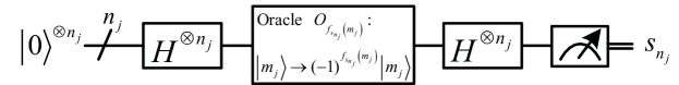
Figure 4: Quantum circuit of DBVA with $t$ computing nodes.

The hidden string $s=s_{n_{0}}s_{n_{1}}\cdots s_{n_{t-1}}\in\{0,1\}^{n}$ will be exactly acquired after following the above algorithm steps. Hence, the entire process of our DBVA with $t$ computing nodes is achieved.

4 Distributed exact Grover’s algorithm

In this section, we mainly describe our distributed exact Grover’s algorithm (DEGA), which decomposes the original search problem into $\lfloor n/2\rfloor$ parts to solve.

4.1 Subfunctions

Similarly, we need to describe our partitioning strategy for the original function before providing our algorithm. We will generate a total of $\lfloor n/2\rfloor$ subfunctions $g_{i}(m_{i})$ for our DEGA, where $i\in\{0,1,\cdots,\lfloor n/2\rfloor-1\}$. The specific generation method is as follows.

When $i\in\{0,1,\cdots,\lfloor n/2\rfloor-2\}$, we choose first $2i$ and last $n-2(i+1)$ bits in $x$ to divide $f$, then we can get $2^{n-2}$ subfunctions $f_{{i},j}:\{0,1\}^{2}\rightarrow\{0,1\}$:

$$f_{{i},j}(m_{i})=f(\underbrace{y_{j_{0}}y_{j_{1}}\cdots y_{j_{2i-1}}}_{2i}m_{i}\underbrace{y_{j_{2i}}y_{j_{2i+1}}\cdots y_{j_{n-3}}}_{n-2(i+1)}),$$ (13)

where $m_{i}\in\{0,1\}^{2}$ and $y_{j_{0}}y_{j_{1}}\cdots y_{j_{2i-1}}y_{j_{2i}}y_{j_{2i+1}}\cdots y_{j_{n-3}}\in\{0,1\}^{n-2}$ is the binary representation of $j\in\{0,1,\cdots,$ $2^{n-2}-1\}$. Afterwards, we generate a new function $g_{i}:\{0,1\}^{2}\rightarrow\{0,1\}$ in terms of these subfunctions,

$$g_{i}(m_{i})=\text{OR}(f_{{i},0}(m_{i}),f_{{i},1}(m_{i}),\cdots,f_{{i},2^{n-2}-1}(m_{i})),$$ (14)

where $m_{i}\in\{0,1\}^{2}$. Besides,

$$\text{OR}(x)=\begin{cases}1,|x|\geq 1,\\ 0,|x|=0,\end{cases}$$ (15)

where $|x|$ is the Hamming weight of $x\in\{0,1\}^{n}$ (its number of 1’s). It means we have acquired $\lfloor n/2\rfloor-1$ subfunctions $g_{i}:\{0,1\}^{2}\rightarrow\{0,1\}$, where $i\in\{0,1,\cdots,\lfloor n/2\rfloor-2\}$.

When $i=\lfloor n/2\rfloor-1$, we choose first $2i$ bits in $x$ to divide $f$, then we can get $2^{2i}$ subfunctions $f_{{i},j}:\{0,1\}^{n-2i}\rightarrow\{0,1\}$:

$$f_{{i},j}(m_{i})=f(\underbrace{y_{j_{0}}y_{j_{1}}\cdots y_{j_{2i-1}}}_{2i}\underbrace{m_{i}}_{n-2i}),$$ (16)

where $m_{i}\in\{0,1\}^{n-2i}$ and $y_{j_{0}}y_{j_{1}}\cdots y_{j_{2i-1}}\in\{0,1\}^{2i}$ is the binary representation of $j\in\{0,1,\cdots,$ $2^{2i}-1\}$. Afterwards, we also generate a new function $g_{i}:\{0,1\}^{n-2i}\rightarrow\{0,1\}$ by means of these subfunctions,

$$g_{i}(m_{i})=\text{OR}(f_{{i},0}(m_{i}),f_{{i},1}(m_{i}),\cdots,f_{{i},2^{2i}-1}(m_{i})),$$ (17)

where $m_{i}\in\{0,1\}^{n-2i}$. Specifically, when $n$ is an even number, we have

$$n-2i=n-2(\lfloor n/2\rfloor-1)=n-2\left(\frac{n}{2}-1\right)=2.$$ (18)

When $n$ is an odd number, we have

$$n-2i=n-2(\lfloor n/2\rfloor-1)=n-2\left(\frac{n-1}{2}-1\right)=3.$$ (19)

4.2 DEGA

So far, we have successfully generated a total of $\lfloor n/2\rfloor$ subfunctions $g_{i}(m_{i})$ according to the original function $f(x)$ and $n$, where $i\in\{0,1,\cdots,$ $\lfloor n/2\rfloor-1\}$. Additionally, we assume that obtaining the Oracle for each subfunction is simple. In other words, we can have $\lfloor n/2\rfloor-1$ Oracles

$$U_{g_{i}(x)}:|x\rangle\rightarrow(-1)^{g_{i}(x)}|x\rangle,$$ (20)

where $x\in\{0,1\}^{2}$, $i\in\{0,1,\cdots,$ $\lfloor n/2\rfloor-2\}$, and $\tau_{i}$ is the target string of $g_{i}(x)$ such that $g_{i}(\tau_{i})=1$.

For the last subfunctions $g_{i}:\{0,1\}^{n-2i}\rightarrow\{0,1\}$, we need to first determine the parity of $n$. If $n$ is an even number, we can also have the Oracle as in Eq. (20), where $i=\lfloor n/2\rfloor-1$. Otherwise, we can have another Oracle

$$R_{g_{i}(x)}:|x\rangle\rightarrow e^{i\phi\cdot g_{i}(x)}|x\rangle,$$ (21)

where $x\in\{0,1\}^{3}$, $i=\lfloor n/2\rfloor-1$, $\tau_{i}$ is the target string of $g_{i}(x)$ such that $g_{i}(\tau_{i})=1$, $\phi=2\arcsin\left(\sin\left(\frac{\pi}{4J+6}\right)/\sin\theta\right)$, $J=\lfloor(\pi/2-\theta)/(2\theta)\rfloor$, and $\theta=\arcsin\left({\sqrt{1/2^{3}}}\right)$.

Next, we provide a detailed introduction to our DEGA in Algorithm 4.2. The whole quantum circuit is shown in Figure 5.

  Algorithm 4 Distributed exact Grover’s algorithm (includes only one target).

 

  Input: (1) The number of qubits $n\geq 2$; (2) A function $f(x)$, where $f(x)=0$ for all $x\in\{0,1\}^{n}$ except $\tau$, for which $f(\tau)=1$; (3) $\lfloor n/2\rfloor$ subfunctions $g_{i}(x)$ as in Eq. (14) and Eq. (17) generated according to $f(x)$ and $n$, where $i\in\{0,1,\cdots,$ $\lfloor n/2\rfloor-1\}$.

  Output: The target index string $\tau=\tau_{0}\tau_{1}\cdots\tau_{\lfloor n/2\rfloor-1}\in\{0,1\}^{n}$ such that $f(\tau)=1$ with a probability of $100\%$.

  Procedure:

  Step 1. Initialize $n$ qubits $|0\rangle^{\otimes n}$.

  Step 2. Apply $n$ Hadamard gates $H^{\otimes n}$.

  Step 3. Let $i=0$.

  Step 4. Execute Grover operator $G_{i}=-H^{\otimes 2}U_{0}H^{\otimes 2}U_{g_{i}(x)}$ once, where $U_{0}=I_{2}-2(|0\rangle\langle 0|)^{\otimes 2}$ and $U_{g_{i}(x)}=I_{2}-2|\tau_{i}\rangle\langle\tau_{i}|$ act on the $(2i)$-th and $(2i+1)$-th qubits, and $\tau_{i}$ is the target string of $g_{i}(x)$ such that $g_{i}(\tau_{i})=1$.

  Step 5. Let $i=i+1$.

  Step 6. Repeat Step 4 to Step 5 until $i=\lfloor n/2\rfloor-1$.

  Step 7. Determine the parity of $n$.

  Step 8. If $n$ is an even number, execute Grover operator $G_{i}=-H^{\otimes 2}U_{0}H^{\otimes 2}U_{g_{i}(x)}$ once, where $U_{0}=I_{2}-2(|0\rangle\langle 0|)^{\otimes 2}$ and $U_{g_{i}(x)}=I_{2}-2|\tau_{i}\rangle\langle\tau_{i}|$ act on the $(2i)$-th and $(2i+1)$-th qubits, and $\tau_{i}$ is the target string of $g_{i}(x)$ such that $g_{i}(\tau_{i})=1$.

  Step 9. If $n$ is an odd number, execute operator $L_{i}=-H^{\otimes 3}R_{0}H^{\otimes 3}R_{g_{i}(x)}$ twice, where $R_{0}=I_{3}+(e^{i\phi}-1)(|0\rangle\langle 0|)^{\otimes 3}$ and $R_{g_{i}(x)}=I_{3}+(e^{i\phi}-1)|\tau_{i}\rangle\langle\tau_{i}|$ act on the $(2i)$-th, $(2i+1)$-th, and $(2i+2)$-th qubits, and $\tau_{i}$ is the target string of $g_{i}(x)$ such that $g_{i}(\tau_{i})=1$.

  Step 10. Measure each qubit in the basis $\{|0\rangle,|1\rangle\}$.

 

The target index string $\tau=\tau_{0}\tau_{1}\cdots\tau_{\lfloor n/2\rfloor-1}\in\{0,1\}^{n}$ will be successfully searched with a probability of $100\%$ after following the above algorithm steps.

Therefore, the entire process of our DEGA is accomplished.

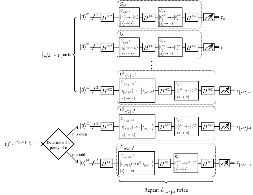
Figure 5: Quantum circuit of DEGA.

5 Analysis

In this section, the analysis of our DBVA and DEGA is presented.

5.1 The degree of $f_{s}(x)$

We demonstrate the degree of $f_{s}(x)$ as in Eq. (1) by the following theorem.

Theorem 1.

The degree $f_{s}(x)$ is $|s|$, where $|s|$ means the Hamming weight of $s$ (its number of 1’s).

Proof.

For the function considering in BV problem:

$$f_{s}(x)=\langle s\cdot x\rangle=\left(\sum_{i=0}^{n-1}s_{i}\cdot x_{i}\right)~{}\text{mod}~{}2,$$ (22)

where $x\in\{0,1\}^{n}$. Once the string $s=s_{0}s_{1}s_{2}\cdots s_{n-1}\in\{0,1\}^{n}$ is determined, then the multilinear polynomial of $f_{s}(x)$ can be expressed as

$$p_{s}(x)=\left(\sum_{i\in\{j|s_{j}=1\}}s_{i}\cdot x_{i}\right)~{}\text{mod}~{}2=\left(\sum_{i\in\{j|s_{j}=1\}}x_{i}\right)~{}\text{mod}~{}2,$$ (23)

where $x\in\{0,1\}^{n}$. Consider the following function,

$$\text{PARITY}_{n}(z)=\left(\sum_{i=0}^{n-1}z_{i}\right)~{}\text{mod}~{}2,$$ (24)

where $z=z_{0}z_{1}z_{2}\cdots z_{n-1}\in\{0,1\}^{n}$. Furthermore, the degree of $\text{PARITY}_{n}(z)$ has been proved to be $n$ [37]. Intuitively, the degree of $f_{s}(x)$ is $|\{j|s_{j}=1\}|=|s|$. Note that $|s|$ means the Hamming weight of $s$ (its number of 1’s).

Therefore, the degree $f_{s}(x)$ is $|s|$. ∎

5.2 Correctness of DBVA

In this subsection, we focus on verifying the correctness of our DBVA. We demonstrate the correctness of Algorithm 3.2 by the following Theorem 2.

Theorem 2.

(Correctness of DBVA) For an $n$-qubit BV problem, suppose that the hidden string $s\in\{0,1\}^{n}$ be expressed as $s=s_{n_{0}}s_{n_{1}}\cdots s_{n_{t-1}}\in\{0,1\}^{n}$, where $s_{n_{j}}\in\{0,1\}^{n_{j}}$ and $\sum_{j=0}^{t-1}n_{j}=n$. We can obtain $s_{j}$ due to Algorithm 3.2, where $j\in\{0,1,\cdots,t-1\}$.

Proof.

It is straightforward. ∎

5.3 Selection of subfunctions

In the previous section, we introduced our partition strategy of the original function. In this subsection, we analyze the selection of subfunctions at the 0-th computing node in DBVA, and similar analysis results can be obtained at other computing nodes.

We choose last $k=n_{1}+n_{2}+\cdots+n_{t-1}$ bits in $x$ to divide $f$, then we can get $2^{k}$ subfunctions $f_{p}:\{0,1\}^{n-k}\rightarrow\{0,1\}$:

$$f_{p}(w) = f(\underbrace{w_{0}w_{1}\cdots w_{n-k-1}}_{n-k}\underbrace{y_{p_{0}}y_{p_{1}}\cdots y_{p_{k-1}}}_{k}),$$ (25)

where $w=w_{0}w_{1}\cdots w_{n-k-1}\in\{0,1\}^{n-k}$, and $y_{p_{0}}y_{p_{1}}\cdots y_{p_{k-1}}\in\{0,1\}^{k}$ is the binary representation of $p\in\{0,1,\cdots,2^{k}-1\}$. We keep the subfunction when $p=0$, and denote it as

$$f_{{s_{n_{0}}}}(m_{0})=f(m_{0}\underbrace{00\cdots 00}_{n_{1}+n_{2}+\cdots+n_{t-1}}),$$ (26)

where $m_{0}\in\{0,1\}^{n_{0}}$.

In fact, no matter which subfunction is selected, the final result will not be affected. For any $p\in\{0,1,\cdots,2^{k}-1\}$, the subfunction $f_{p}(w)$ will be determined accordingly, the final substring is always $s_{0}s_{1}\dots s_{n-k}\in\{0,1\}^{n-k}$.

The similar analysis results can be obtained at other computing nodes.

5.4 The depth of circuir

In order to compare the circuit depth, we give the following definition.

Definition 1.

(Depth of circuit) The depth of circuit is defined as the longest path from the input to the output, moving forward in time along qubit wires.

The depth of the circuit on the left, for example, is 1, whereas the right is 11. (see Figure 6)

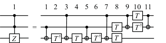
Figure 6: Equivalent quantum circuit of Toffoli gate (or $C^{2}Z$ gate), where $T$ represent $\pi/8$ gate and $T^{\dagger}$ represents the conjugate transpose of $T$.

In the process of building the circuit of BV algorithm, we will run into an issue of how to construct the Oracle required by the algorithm. Due to the algorithm for constructing quantum circuits to realizing Oracle by Qiu et al. [33], we here have the construction for the Oracles immediately as follows.

Given a function $f:\{0,1\}^{n}\rightarrow\{0,1\}$. Suppose there are $k$ inputs $x^{(i)}=(x_{0}x_{1}\cdots x_{n-1})^{(i)}$ satisfying $f(x^{(i)})=1$, where $i\in\{0,1,\cdots,k-1\}$. The Oracle construction is as follows:

Step 1. Let $i=0$.

Step 2. For $x^{(i)}$, execute Pauli $X$ gate on $j$-th qubit if $(x_{j})^{(i)}=0$, otherwise execute identity gate $I$, where $j\in\{0,1,\cdots,n-1\}$.

Step 3. Apply $C^{n-1}Z$ gate once.

Step 4. Execute the same operation as in Step 2.

Step 5. Let $i=i+1$.

Step 6. Repeat Step 2 to Step 5 until $i=k$.

Step 7. Summarize all quantum gates in the above steps.

Following the above steps, we can easily construct the quantum circuit corresponding to Oracle $O_{f}$.

For example, a Boolean function $f:\{0,1\}^{3}\rightarrow\{0,1\}$ is defined as follows:

$$f(x)=\begin{cases}1,x=010,101,\\ 0,\text{otherwise}.\end{cases}$$ (27)

According to the above method, its corresponding Oracle $O_{f}$ quantum circuit is shown below (see Figure 7).

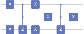
Figure 7: Quantum circuit corresponding to Oracle $O_{f}$ in the example.

Once we figure out how to build the circuit realizing Oracle, we can get the circuit depth of BV algorithm. We need the following lemma.

Lemma 1.

For any $s=s_{0}s_{1}s_{2}\dots s_{n-1}\in\{0,1\}^{n}/0^{n}$, we have $|\{x|f_{s}(x)=1\}|=2^{n-1}$, where $f_{s}(x)$ as in Eq. (1).

Proof.

First of all, $f_{s}(x)=\langle s\cdot x\rangle=\left(\sum_{i=0}^{n-1}s_{i}\cdot x_{i}\right)~{}\text{mod}~{}2:\{0,1\}^{n}\rightarrow\{0,1\}$, where $s\in\{0,1\}^{n}$. Suppose $k\neq 0$ bits in $s$ are 1, and the rest are 0. Without loss of generality, for the purpose of analysis, $s$ can be rearranged so that the bits with the value of 1 are all on the left, as shown below

$$s = \underbrace{s_{i_{0}}s_{i_{1}}\cdots s_{i_{k-1}}}_{k}\underbrace{s_{j_{0}}s_{j_{1}}\cdots s_{j_{n-k-1}}}_{n-k}$$ (28)

$$= \underbrace{11\cdots 11}_{k}\underbrace{00\cdots 00}_{n-k}.$$

Then we have

$$f_{s}(x) = \left(\sum_{i=0}^{k-1}1\cdot x_{i}+\sum_{i=k}^{n-1}0\cdot x_{i}\right)~{}\text{mod}~{}2$$ (29)

$$= \left(\sum_{i=0}^{k-1}x_{i}\right)~{}\text{mod}~{}2.$$

It means that once we determine the first $k$ bits in $x\in\{0,1\}^{n}$, no matter what the value of the last $n-k$ bits in $x$ is, it will not affect the final function value. Therefore, we can regard Eq. (29) as a parity function: $\{0,1\}^{k}\rightarrow\{0,1\}$:

$$\text{PARITY}_{k}(z)=\left(\sum_{i=0}^{k-1}z_{i}\right)~{}\text{mod}~{}2.$$ (30)

Obviously, since $\text{PARITY}_{k}(z)$ is a balanced function (half of the inputs will output 0, and the other will output 1), there are $2^{k-1}$ strings such that $\text{PARITY}_{k}(z)=1$. Finally, we add the remaining $n-k$ bits, which means there are $2^{k-1}\cdot 2^{n-k}=2^{n-1}$ strings making $f_{s}(x)=1$. In other words, we have $|\{x|f_{s}(x)=1\}|=2^{n-1}$. ∎

We can build a complete quantum circuit of BV algorithm by the Oracle construction method introduced above. According to Lemma 1, there are $2^{n-1}$ target states that need to flip the phase. Furthermore, we should execute a quantum circuit with a circuit depth of 3 to realize phase flipping of a target state. In addition, $H^{\otimes n}$ needs to be executed twice. So the circuit depth of the BV algorithm satisfies

$$dep(\text{BV}) =\begin{cases}3\cdot 2^{n-1}+2,&\text{target states do not contain}~{}|1\rangle^{\otimes n},\\ 3\cdot 2^{n-1}-2+2,&\text{target states contain}~{}|1\rangle^{\otimes n},\end{cases}$$ (31)

$$=\begin{cases}3\cdot 2^{n-1}+2,&\text{target states do not contain}~{}|1\rangle^{\otimes n},\\ 3\cdot 2^{n-1},&\text{target states contain}~{}|1\rangle^{\otimes n},\end{cases}$$

$$\leq 3\cdot 2^{n-1}+2$$

When the target states contain $|1\rangle^{\otimes n}$, it is not necessary to execute Step 2 and Step 4 of the Oracle construction circuit during flipping the phase of $|1\rangle^{\otimes n}$. So the circuit depth can be reduced by 2.

Additionally, since $X$ gate can be executed in parallel on different qubits and $X^{2}=I$, the circuit can be further optimized. For example, the circuit depth of Figure 7 is 6 before optimization and 5 after optimization. Thus, the circuit depth of BV algorithm after optimization satisfies

$$dep(\text{BV, optimized}) =\begin{cases}2\cdot 2^{n-1}+1+2,&\text{target states do not contain}~{}|1\rangle^{\otimes n},\\ 2\cdot 2^{n-1}+1-1+2,&\text{target states contain}~{}|1\rangle^{\otimes n},\end{cases}$$ (32)

$$=\begin{cases}2^{n}+3,&\text{target states do not contain}~{}|1\rangle^{\otimes n},\\ 2^{n}+2,&\text{target states contain}~{}|1\rangle^{\otimes n},\end{cases}$$

$$\leq 2^{n}+3.$$

Similarly, we can get the circuit depth of DBVA by the following theorem.

Theorem 3.

The circuit depth of Algorithm 3.2 is not greater than $2^{\text{max}(n_{0},n_{1},\cdots,n_{t-1})}+3$.

Proof.

Since each computing node will execute a quantum circuit of small-scale BV algorithm, we just need to consider the computing node with the largest number when calculating the circuit depth. Therefore, we can know that the circuit depth of DBVA after optimization satisfies

$$dep(\text{DBVA, optimized})\leq 2^{\text{max}(n_{0},n_{1},\cdots,n_{t-1})}+3.$$ (33)

When the target states do not contain $|1\rangle^{\otimes\text{max}(n_{0},n_{1},\cdots,n_{t-1})}$, the equal sign is true. When the target states contain $|1\rangle^{\otimes\text{max}(n_{0},n_{1},\cdots,n_{t-1})}$, the circuit depth can be $2^{\text{max}(n_{0},n_{1},\cdots,n_{t-1})}+2$. ∎

5.5 Correctness of DEGA

To verify the correctness of our DEGA, it is equivalent to proving that we can obtain the target index string $\tau\in\{0,1\}^{n}$ by Algorithm 4.2 with a probability of $100\%$. Firstly, we give the following theorem.

Theorem 4.

Each subfunction $g_{i}(x)$ (as in Eq. (14) and Eq. (17)) has its corresponding target string $\tau_{i}$ such that $g_{i}(\tau_{i})=1$, which satisfies

$$\tau=\tau_{0}\tau_{1}\cdots\tau_{\lfloor n/2\rfloor-1},$$ (34)

where $i\in\{0,1,\cdots,$ $\lfloor n/2\rfloor-1\}$ and $\tau\in\{0,1\}^{n}$ is the target string of the original function $f(x)$.

Proof.

The method of proof is simple, so we omit the details. ∎

So far, we have proved that the target string corresponding to each subfunction $g_{i}(m_{i})$ is $\tau_{i}$, which satisfies $\tau=\tau_{0}\tau_{1}\cdots\tau_{\lfloor n/2\rfloor-1}$, where $i\in\{0,1,\cdots,$ $\lfloor n/2\rfloor-1\}$.

Next, we demonstrate the correctness of Algorithm 4.2 by the following Theorem 5.

Theorem 5.

(Correctness of DEGA) For an $n$-qubit search problem that includes only one target index string, suppose that the goal can be expressed as $\tau=x_{0}x_{1}\cdots x_{n-1}\in\{0,1\}^{n}$ of the original function $f(x)$. Then we can obtain $\tau=\tau_{0}\tau_{1}\cdots\tau_{\lfloor n/2\rfloor-1}$ by Algorithm 4.2 with a probability of $100\%$, where $\tau_{i}$ is the target string of $g_{i}(x)$ and satisfies

$$\tau_{i}=\begin{cases}x_{2i}x_{2i+1},&i\in\{0,1,\cdots,$ $\lfloor n/2\rfloor-2\},\\ x_{2i}x_{2i+1}\cdots x_{n-1}=\begin{cases}x_{2i}x_{2i+1}=x_{n-2}x_{n-1},&n~{}\text{is even},\\ x_{2i}x_{2i+1}x_{2i+2}=x_{n-3}x_{n-2}x_{n-1},&n~{}\text{is odd},\end{cases},&i=\lfloor n/2\rfloor-1.\end{cases}$$ (35)

Proof.

From subsection 4.1, we have declared how to generate $\lfloor n/2\rfloor$ subfunctions $g_{i}(x)$ as in Eq. (14) and Eq. (17) according to $f(x)$ and $n$, which decomposes the original search problem into $\lfloor n/2\rfloor$ parts to solve, where $i\in\{0,1,\cdots,$ $\lfloor n/2\rfloor-1\}$.

Furthermore, suppose that the goal can be expressed as $\tau=x_{0}x_{1}\cdots x_{n-1}\in\{0,1\}^{n}$ of the original function $f(x)$. Theorem 4 has already explained each subfunction $g_{i}(x)$ has its corresponding target string $\tau_{i}$ such that $g_{i}(\tau_{i})=1$, which satisfies

$$\tau=\tau_{0}\tau_{1}\cdots\tau_{\lfloor n/2\rfloor-1}.$$ (36)

Last but not least, we will accurately obtain the solution of each part. For $i\in\{0,1,\cdots,$ $\lfloor n/2\rfloor-2\}$, by running the 2-qubit Grover’s algorithm, we can precisely determine $\tau_{i}=x_{2i}x_{2i+1}\in\{0,1\}^{2}$. For $i=\lfloor n/2\rfloor-1$, by running the 2-qubit Grover’s algorithm when $n$ is even or the 3-qubit algorithm by Long when $n$ is odd, we can exactly obtain

$$\tau_{i}=x_{2i}x_{2i+1}\cdots x_{n-1}=\begin{cases}x_{2i}x_{2i+1}=x_{n-2}x_{n-1}\in\{0,1\}^{2},&n~{}\text{is even},\\ x_{2i}x_{2i+1}x_{2i+2}=x_{n-3}x_{n-2}x_{n-1}\in\{0,1\}^{3},&n~{}\text{is odd}.\end{cases}$$ (37)

In conclusion, we can obtain $\tau=\tau_{0}\tau_{1}\cdots\tau_{\lfloor n/2\rfloor-1}$ by Algorithm 4.2 with a probability of $100\%$, where $\tau_{i}$ is the target string of $g_{i}(x)$, where $i\in\{0,1,\cdots,$ $\lfloor n/2\rfloor-1\}$. ∎

5.6 Comparison

In order to compare the circuit depth, we will introduce a general construction for the Oracles in Grover’s algorithm.

$U_{f(x)}=I_{n}-2|\tau\rangle\langle\tau|$ is employed in the Grover operator $G=-H^{\otimes n}U_{0}H^{\otimes n}U_{f(x)}$ to flip the phase of the target state $|\tau\rangle=|x_{0}x_{1}\cdots x_{n-1}\rangle$, where $\tau=x_{0}x_{1}\cdots x_{n-1}\in\{0,1\}^{n}$. Thus, the specific construction circuit of $U_{f(x)}$ (see Figure 9) is as follows:

$$O_{U_{f(x)}}=\left(\bigotimes_{i=0}^{n-1}X^{1-x_{i}}\right)\left(C^{n-1}Z\right)\left(\bigotimes_{i=0}^{n-1}X^{1-x_{i}}\right),$$ (38)

where $X$ and $Z$ represent the Pauli-$X$ and Pauli-$Z$ gates, and $C^{n-1}Z$ will only flip the phase of $|1\rangle^{\otimes n}$,

$$\left(C^{n-1}Z\right)|x\rangle=\begin{cases}-|x\rangle,&|x\rangle=|1\rangle^{\otimes n},\\ |x\rangle,&\text{otherwise},\end{cases}$$ (39)

where $x=x_{0}x_{1}\cdots x_{n-1}\in\{0,1\}^{n}$. Besides, it should be noted that

$$X^{1-x_{i}}=\begin{cases}X,&x_{i}=0,\\ I,&x_{i}=1,\end{cases}$$ (40)

where $i\in\{0,1,\cdots,n-1\}$. In particular, the construction circuit of $U_{0}=I_{n}-2(|0\rangle\langle 0|)^{\otimes n}$ (see Figure 9) is

$$O_{U_{0}}=\left(X^{\otimes n}\right)\left(C^{n-1}Z\right)\left(X^{\otimes n}\right).$$ (41)

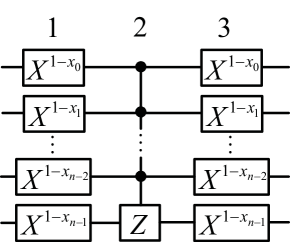
Figure 8: The quantum circuit corresponding to the Oracle $O_{U_{f(x)}}$.

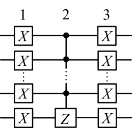
Figure 9: The quantum circuit corresponding to the Oracle $O_{U_{0}}$.

It can be found that the quantum circuit in Figure 9 or Figure 9 has a circuit depth of 3.

Similarly, we can also give the specific construction circuit of $R_{f(x)}=I_{n}+(e^{i\phi}-1)|\tau\rangle\langle\tau|$ with $L=-H^{\otimes n}R_{0}H^{\otimes n}R_{f(x)}$ (see Figure 11) as follows:

$$O_{R_{f(x)}}=\left(\bigotimes_{i=0}^{n-1}X^{1-x_{i}}\right)\left(C^{n-1}R(\phi)\right)\left(\bigotimes_{i=0}^{n-1}X^{1-x_{i}}\right),$$ (42)

where $R(\phi)$ represents the rotation gate,

$$R(\phi)=\left(\begin{array}[]{cc}1&0\\ 0&e^{i\phi}\end{array}\right),$$ (43)

and $C^{n-1}R(\phi)$ will only rotate the phase of $|1\rangle^{\otimes n}$,

$$\left(C^{n-1}R(\phi)\right)|x\rangle=\begin{cases}e^{i\phi}|x\rangle,&|x\rangle=|1\rangle^{\otimes n},\\ |x\rangle,&\text{otherwise},\end{cases}$$ (44)

where $x=x_{0}x_{1}\cdots x_{n-1}\in\{0,1\}^{n}$. In particular, the construction circuit of $R_{0}=I_{n}+(e^{i\phi}-1)(|0\rangle\langle 0|)^{\otimes n}$ is

$$O_{R_{0}}=\left(X^{\otimes n}\right)\left(C^{n-1}R(\phi)\right)\left(X^{\otimes n}\right).$$ (45)

It can be found that the quantum circuits in Figure 11 or Figure 11 also have a circuit depth of 3.

After identifying the specific quantum gates in Grover’s algorithm and the algorithm by Long, we might calculate the circuit depth of these two methods.

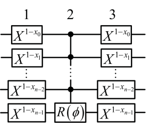
Figure 10: The quantum circuit corresponding to the Oracle $O_{R_{f(x)}}$.

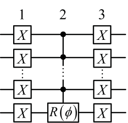
Figure 11: The quantum circuit corresponding to the Oracle $O_{R_{0}}$.

Theorem 6.

The circuit depths for Grover’s algorithm and the algorithm by Long are $1+8\left\lfloor\frac{\pi}{4}\sqrt{2^{n}}\right\rfloor$ and $9+8\left(\left\lfloor\frac{\pi}{4}\sqrt{2^{n}}-\frac{1}{2}\right\rfloor\right)$, respectively.

Proof.

In the Grover’s algorithm, Grover operator $G=-H^{\otimes n}U_{0}H^{\otimes n}U_{f(x)}$ is executed with $\left\lfloor\frac{\pi}{4}\sqrt{2^{n}}\right\rfloor$ times, where $dep(U_{f})=dep(U_{0})=3$ and $dep(H^{\otimes n})=1$. Thus, the circuit depth of Grover’s algorithm is

$$dep(\text{Grover}) = 1+\left\lfloor\frac{\pi}{4}\sqrt{2^{n}}\right\rfloor*(3+1+3+1)$$ (46)

$$= 1+8\left\lfloor\frac{\pi}{4}\sqrt{2^{n}}\right\rfloor.$$

Similarly, since the operator $L=-H^{\otimes n}R_{0}H^{\otimes n}R_{f(x)}$ in the algorithm by Long is executed with $J+1$ times, where $J=\lfloor(\pi/2-\theta)/(2\theta)\rfloor$, $\theta=\arcsin\left(\sqrt{1/2^{n}}\right)$, and $dep(R_{f})=dep(R_{0})=3$, the circuit depth of the algorithm by Long is

$$dep(\text{Long}) = 1+\left(\left\lfloor\frac{\pi}{4}\sqrt{2^{n}}-\frac{1}{2}\right\rfloor+1\right)*(3+1+3+1)$$ (47)

$$= 9+8\left(\left\lfloor\frac{\pi}{4}\sqrt{2^{n}}-\frac{1}{2}\right\rfloor\right).$$

∎

Next, we give the circuit depth of our DEGA by the following theorem.

Theorem 7.

The circuit depth of Algorithm 4.2 is $8(n~{}\text{mod}~{}2)+9$.

Proof.

When $n$ is an even number, our DEGA will run $\lfloor n/2\rfloor$ parts 2-qubit Grover’s algorithm, and each part only needs to iterate the Grover operator $G$ once, so the circuit depth is

$$dep(\text{DEGA},n~{}\text{is even})=1+1*(3+1+3+1)=9.$$ (48)

When $n$ is an odd number, our DEGA will run $\lfloor n/2\rfloor-1$ parts 2-qubit Grover’s algorithm and 1 part 3-qubit algorithm by Long, and the last part needs to iterate the operator $L$ twice, so the circuit depth is

$$dep(\text{DEGA},n~{}\text{is odd})=1+2*(3+1+3+1)=17.$$ (49)

In other words, the actual depth of our circuit is

$$dep(\text{DEGA})=8(n~{}\text{mod}~{}2)+9=\begin{cases}9,&n~{}\text{is even},\\ 17,&n~{}\text{is odd}.\end{cases}$$ (50)

∎

Therefore, the actual circuit depth will be shallower compared with the original Grover’s and the algorithm by Long. The circuit depth of our DEGA only depends on the parity of $n$, and it is not deepened as $n$ increases.

Next, we will contrast our DEGA with the existing distributed Grover’s algorithms.

In [33], Qiu et al. presented the serial and parallel distributed Grover’s algorithms and divided the original function $f$ into $2^{k}$ subfunctions $f_{p}:\{0,1\}^{n-k}\rightarrow\{0,1\}$ as in Eq. (6), where $2^{k}$ represents the number of computing nodes. In particular, the method in [33] can solve the search problem having multiple objectives, but in the present paper we must realize the search problem only having unique objective, otherwise we cannot solve it here. The total number of qubits used in their parallel scheme by Qiu et al. is $2^{k}(n-k)$.

6 Experiment

In this section, we provide particular situations of our DBVA and DEGA on MindQuantum.

6.1 The Bernstein-Vazirani algorithm, the hidden string $s=001011$

Let Boolean function $f:\{0,1\}^{6}\rightarrow\{0,1\}$. Consider a function $f_{s}(x)=\langle s\cdot x\rangle=(\sum_{i=0}^{5}s_{i}\cdot x_{i})~{}\text{mod}~{}2$, where $x\in\{0,1\}^{6}$. Suppose the hidden string we want to find is $s=001011$. The function values corresponding to all input strings are shown in TABLE 1. Then we can build a complete quantum circuit of the BV algorithm (see Figure 12).

$i$	$x^{(i)}$	$f_{s}(x^{(i)})$	$i$	$x^{(i)}$	$f_{s}(x^{(i)})$	$i$	$x^{(i)}$	$f_{s}(x^{(i)})$	$i$	$x^{(i)}$	$f_{s}(x^{(i)})$
0	000000	0	16	010000	0	32	100000	0	48	110000	0
1	000001	1	17	010001	1	33	100001	1	49	110001	1
2	000010	1	18	010010	1	34	100010	1	50	110010	1
3	000011	0	19	010011	0	35	100011	0	51	110011	0
4	000100	0	20	010100	0	36	100100	0	52	110100	0
5	000101	1	21	010101	1	37	100101	1	53	110101	1
6	000110	1	22	010110	1	38	100110	1	54	110110	1
7	000111	0	23	010111	0	39	100111	0	55	110111	0
8	001000	1	24	011000	1	40	101000	1	56	111000	1
9	001001	0	25	011001	0	41	101001	0	57	111001	0
10	001010	0	26	011010	0	42	101010	0	58	111010	0
11	001011	1	27	011011	1	43	101011	1	59	111011	1
12	001100	1	28	011100	1	44	101100	1	60	111100	1
13	001101	0	29	011101	0	45	101101	0	61	111101	0
14	001110	0	30	011110	0	46	101110	0	62	111110	0
15	001111	1	31	011111	1	47	101111	1	63	111111	1

Table 1: Function value of original function $f_{s}(x)$.

Figure 12: The quantum circuit of BV algorithm.

Furthermore, the above circuit can be further optimized (see Figure 13).

Figure 13: The quantum circuit of the BV algorithm after optimization.

The total number of quantum gates before optimization is 236, and after optimization is 130. The circuit depth is reduced from 96 to 66 after optimization.

Sampling the circuit 10,000 times, the results can be found in Figure 14.

Figure 14: The sampling results of BV algorithm after optimization.

The sampling results demonstrate that $s=001011$ is obtained after measurement.

6.2 The DBVA with two computing nodes, the hidden string $s=001011$

The next step is to examine the quantum circuit of our DBVA with two computing nodes. Here, computing nodes $t=2$, and the number of qubits per computing node $n_{0}=n_{1}=3$.

Firstly, generate two subfunctions $f_{s_{n_{0}}}(y)$ and $f_{s_{n_{1}}}(y)$ according to function $f_{s}(x)$:

$$f_{s_{n_{0}}}(y) = f_{s}(y000),$$ (51)

$$f_{s_{n_{1}}}(y) = f_{s}(000y),$$ (52)

where $y\in\{0,1\}^{3}$. Each subfunction value for all input strings is shown in TABLE 2.

$i$	$y^{(i)}$	$f_{s_{n_{0}}}\left(y^{(i)}\right)$	$f_{s_{n_{1}}}\left(y^{(i)}\right)$
0	000	0	0
1	001	1	1
2	010	0	1
3	011	1	0
4	100	0	0
5	101	1	1
6	110	0	1
7	111	1	0

Table 2: Function values of subfunctions $f_{s_{n_{0}}}(y)=f_{s}(y000)$ and $f_{s_{n_{1}}}(y)=f_{s}(000y)$.

We build the complete quantum circuit of our DBVA with two computing nodes (see Figure 15). Note that since the reading order on MindQuantum is from right to left, which is the opposite of our reading order from left to right, the 3-qubit BV algorithm corresponding to $f_{s_{n_{1}}}(y)$ is located on the top of the circuit.

Furthermore, the optimized quantum circuit can be obtained (see Figure 16).

The total number of quantum gates before optimization is 40, and after optimization is 36. The circuit depth is reduced from 14 to 11 after optimization.

By sampling the circuit 10,000 times, the results can be found in Figure 17.

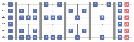
Figure 15: The quantum circuit of DBVA with two computing nodes.

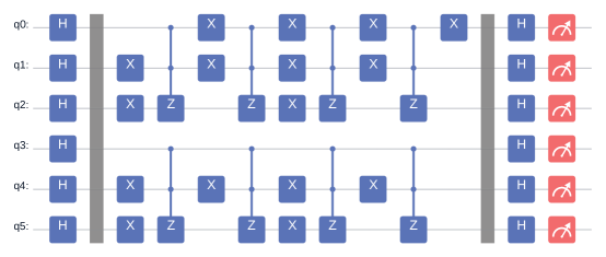
Figure 16: The quantum circuit of DBVA with two computing nodes after optimization.

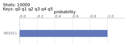
Figure 17: The sampling results of DBVA with two computing nodes after optimization.

As can be seen from the sampling results, we definitely obtain the hidden string $s=s_{n_{0}}s_{n_{1}}=001011$ after our DBVA with two computing nodes, which is the same as the result of the original BV algorithm.

6.3 The DBVA with $t=3$ computing nodes, the hidden string $s=001011$

Further, we consider the experiment of our DBVA with $t=3$ computing nodes. Here, computing nodes $t=3$, and the number of qubits per computing node $n_{0}=n_{1}=n_{2}=2$.

Firstly, generate three subfunctions $f_{s_{n_{0}}}(m)$, $f_{s_{n_{1}}}(m)$, and $f_{s_{n_{2}}}(m)$ according to function $f_{s}(x)$:

$$f_{s_{n_{0}}}(m) = f(m0000),$$ (53)

$$f_{s_{n_{1}}}(m) = f(00m00),$$ (54)

$$f_{s_{n_{2}}}(m) = f(0000m),$$ (55)

where $m\in\{0,1\}^{2}$. Each subfunction value for all input strings is shown in TABLE 3.

$i$	$m^{(i)}$	$f_{s_{n_{0}}}\left(m^{(i)}\right)$	$f_{s_{n_{1}}}\left(m^{(i)}\right)$	$f_{s_{n_{2}}}\left(m^{(i)}\right)$
0	00	0	0	0
1	01	0	0	1
2	10	0	1	1
3	11	0	1	0

Table 3: Function values of subfunctions $f_{s_{n_{0}}}=f(m0000)$, $f_{s_{n_{1}}}(m)=f(00m00)$, $f_{s_{n_{2}}}(m)=f(0000m)$.

We can easily draw the whole quantum circuit of our DBVA with $t=3$ computing nodes (see Figure 19). The 2-qubit BV algorithms corresponding to $f_{s_{n_{2}}}(y)$, $f_{s_{n_{1}}}(y)$ and $f_{s_{n_{0}}}(y)$ are located at the top, middle and bottom of the circuit respectively.

The number of quantum gates is 22 and the circuit depth is 7. By sampling the circuit 10,000 times, the results can be found in Figure 19.

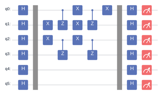
Figure 18: The quantum circuit of DBVA with $t=3$ computing nodes.

Figure 19: The sampling results of DBVA with $t=3$ computing nodes after optimization.

As can be seen from the sampling results, we definitely obtain the hidden string $s=s_{n_{0}}s_{n_{1}}s_{n_{2}}=001011$ after our DBVA with $t=3$ computing nodes, which is the same as the result of the original BV algorithm.

It can be found that the final result of DBVA with two or three computing nodes is consistent with the result of the original BV algorithm. However, DBVA requires fewer quantum gates and has a shallower circuit depth (see TABLE 4). With the increase of the number of computing nodes (from 2 to 3), the number of quantum gates and the circuit depth are further reduced.

	BV	optimized BV	DBVA-2	optimized DBVA-2	optimized DBVA-3
1. The number of computing nodes	1	1	2	2	3
2. Figure number	Figure 12	Figure 13	Figure 15	Figure 16	Figure 19
3. Final result	001011	001011	001011	001011	001011
4. The number of quantum gates	236	130	40	36	22
5. The circuit depth	96	66	14	11	7

Table 4: A simple comparison between our DBVA and the original BV algorithm.

6.4 The 2-qubit DEGA, the target string $\tau=01$

Let Boolean function $f:\{0,1\}^{2}\rightarrow\{0,1\}$. Suppose

$$f(x)=\begin{cases}1,x=01,\\ 0,x\neq 01,\end{cases}$$ (56)

where $x\in\{0,1\}^{2}$ and $\tau=01$ is the target string. When $n=2$, our DEGA is a 2-qubit Grover’s algorithm. Thus, we can build its circuit (see Figure 21). By sampling the circuit 10,000 times, the results can be found in Figure 21. The total number of quantum gates is 14 and the circuit depth is 9.

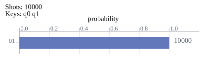
Figure 20: The quantum circuit of the 2-qubit Grover’s algorithm (target string $\tau=01$).

Figure 21: The sampling results of the 2-qubit Grover’s algorithm (target string $\tau=01$).

The sampling results demonstrate that $\tau=01$ is obtained exactly after measurement.

6.5 The 3-qubit DEGA, the target string $\tau=101$

Let Boolean function $f:\{0,1\}^{3}\rightarrow\{0,1\}$. Suppose

$$f(x)=\begin{cases}1,x=101,\\ 0,x\neq 101,\end{cases}$$ (57)

where $x\in\{0,1\}^{3}$ and $\tau=101$ is the target string. When $n=3$, our DEGA is a 3-qubit algorithm by Long. Thus, we can build its circuit (see Figure 23). By sampling the circuit 10,000 times, the results can be found in Figure 23. Note that PhaseShift (called the PS gate) is a single-qubit gate, whose matric is as follows

$$\text{PS($\phi$)}=\left(\begin{array}[]{cc}1&0\\ 0&e^{i\phi}\end{array}\right).$$ (60)

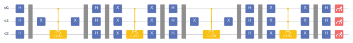
Figure 22: The quantum circuit of the 3-qubit algorithm by Long (target string $\tau=101$). The parameter in the circuit is $\phi=2\arcsin\left(\sin\left(\frac{\pi}{4J+6}\right)/\sin\theta\right)=2.1268800471555034\approx 2.1269$, where $J=\lfloor(\pi/2-\theta)/(2\theta)\rfloor$ and $\theta=\arcsin{\sqrt{1/2^{3}}}$.

Figure 23: The sampling results of the 3-qubit algorithm by Long (target string $\tau=101$).

The total number of quantum gates is 35 and the circuit depth is 17.

The sampling results demonstrate that $\tau=101$ is obtained exactly after measurement.

6.6 The 4-qubit DEGA, the target string $\tau=1001$

Let Boolean function $f:\{0,1\}^{4}\rightarrow\{0,1\}$. Suppose

$$f(x)=\begin{cases}1,x=1001,\\ 0,x\neq 1001,\end{cases}$$ (61)

where $x\in\{0,1\}^{4}$ and $\tau=1001$ is the target string. When $n=4$, we can decomposes the original search problem into $\lfloor n/2\rfloor=2$ parts to solve. To be specific, we choose last $2$ bits in $x$ to divide $f$, then we can get $2^{2}=4$ subfunctions $f_{{0},j}:\{0,1\}^{2}\rightarrow\{0,1\}$:

$$f_{{0},0}(m_{0}) = f(m_{0}00),$$ (62)

$$f_{{0},1}(m_{0}) = f(m_{0}01),$$ (63)

$$f_{{0},2}(m_{0}) = f(m_{0}10),$$ (64)

$$f_{{0},3}(m_{0}) = f(m_{0}11),$$ (65)

where $m_{0}\in\{0,1\}^{2}$ and $j\in\{0,1,2,3\}$. Obviously, $f_{{0},0}(m_{0})=f_{{0},2}(m_{0})=f_{{0},3}(m_{0})\equiv 0$, and

$$f_{{0},1}(m_{0})=\begin{cases}1,m_{0}=10,\\ 0,m_{0}\neq 10,\end{cases}$$ (66)

where $m_{0}\in\{0,1\}^{2}$ and $10$ is the target substring.

Afterwards, we generate a new function $g_{0}:\{0,1\}^{2}\rightarrow\{0,1\}$ in terms of above four subfunctions,

$$g_{0}(m_{0})=\text{OR}\left(f_{{0},0}(m_{0}),f_{{0},1}(m_{0}),f_{{0},2}(m_{0}),f_{{0},3}(m_{0})\right)=\begin{cases}1,m_{0}=10,\\ 0,m_{0}\neq 10,\end{cases}$$ (67)

where $m_{0}\in\{0,1\}^{2}$.

Similarly, we choose first $2$ bits in $x$ to divide $f$, then we can get $2^{2}=4$ subfunctions $f_{{1},j}:\{0,1\}^{2}\rightarrow\{0,1\}$:

$$f_{{1},0}(m_{1}) = f(00m_{1}),$$ (68)

$$f_{{1},1}(m_{1}) = f(01m_{1}),$$ (69)

$$f_{{1},2}(m_{1}) = f(10m_{1}),$$ (70)

$$f_{{1},3}(m_{1}) = f(11m_{1}),$$ (71)

where $m_{1}\in\{0,1\}^{2}$ and $j\in\{0,1,2,3\}$. Obviously, $f_{{1},0}(m_{1})=f_{{1},1}(m_{1})=f_{{1},3}(m_{1})\equiv 0$, and

$$f_{{1},2}(m_{1})=\begin{cases}1,m_{1}=01,\\ 0,m_{1}\neq 01,\end{cases}$$ (72)

where $m_{1}\in\{0,1\}^{2}$ and $01$ is the target substring.

Afterwards, we generate a new function $g_{1}:\{0,1\}^{2}\rightarrow\{0,1\}$ in terms of above four subfunctions,

$$g_{1}(m_{1})=\text{OR}\left(f_{{1},0}(m_{1}),f_{{1},1}(m_{1}),f_{{1},2}(m_{1}),f_{{1},3}(m_{1})\right)=\begin{cases}1,m_{1}=01,\\ 0,m_{1}\neq 01,\end{cases}$$ (73)

where $m_{1}\in\{0,1\}^{2}$.

Next, we can build the completed circuit (see Figure 24). The 2-qubit Grover’s algorithm corresponding to $g_{1}(m_{1})$ is located on the top of the circuit. By sampling the circuit 10,000 times, the results can be found in Figure 25.

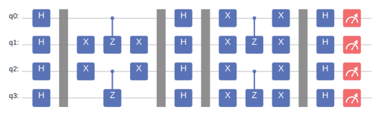
Figure 24: The quantum circuit of the 4-qubit DEGA (target string $\tau=1001$).

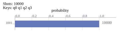
Figure 25: The sampling results of the 4-qubit DEGA (target string $\tau=1001$).

The total number of quantum gates is 28 and the circuit depth is 9.

The sampling results demonstrate that $\tau=1001$ is obtained exactly after measurement.

If the Grover’s algorithm or the algorithm by Long is employed to search 1001, we can build the completed circuits (see Figure 27 and Figure 27) respectively. By sampling the circuits 10,000 times respectively, the results can be found in Figure 29 and Figure 29. The number of quantum gates required by two algorithms is 70, and the circuit depth is 25.

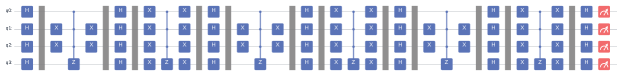
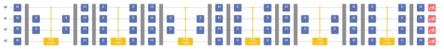
Figure 26: The quantum circuit of the 4-qubit Grover’s algorithm (target string $\tau=1001$).

Figure 27: The quantum circuit of the 4-qubit algorithm by Long (target string $\tau=1001$). The parameter in the circuit is $\phi=2\arcsin\left(\sin\left(\frac{\pi}{4J+6}\right)/\sin\theta\right)=2.195057699090115\approx 2.1951$, where $J=\lfloor(\pi/2-\theta)/(2\theta)\rfloor$ and $\theta=\arcsin{\sqrt{1/2^{4}}}$.

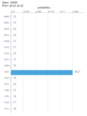
Figure 28: The sampling results of the 4-qubit Grover’s algorithm (target string $\tau=1001$).

Figure 29: The sampling results of the 4-qubit algorithm by Long (target string $\tau=1001$).

It can be found that the probability of the Grover’s algorithm acquiring target string $\tau=1001$ is 0.9627, which is not exact, while the algorithm by Long can accurately obtain $\tau=1001$.

6.7 The 5-qubit DEGA, the target string $\tau=01001$

Let Boolean function $f:\{0,1\}^{5}\rightarrow\{0,1\}$. Suppose

$$f(x)=\begin{cases}1,x=01001,\\ 0,x\neq 01001,\end{cases}$$ (74)

where $x\in\{0,1\}^{5}$ and $\tau=01001$ is the target string. When $n=5$, we can decomposes the original search problem into $\lfloor n/2\rfloor=2$ parts to solve. To be specific, we choose last $2$ bits in $x$ to divide $f$, then we can get $2^{2}=4$ subfunctions $f_{{0},j}:\{0,1\}^{3}\rightarrow\{0,1\}$:

$$f_{{0},0}(m_{0}) = f(m_{0}00),$$ (75)

$$f_{{0},1}(m_{0}) = f(m_{0}01),$$ (76)

$$f_{{0},2}(m_{0}) = f(m_{0}10),$$ (77)

$$f_{{0},3}(m_{0}) = f(m_{0}11),$$ (78)

where $m_{0}\in\{0,1\}^{3}$ and $j\in\{0,1,2,3\}$. Obviously, $f_{{0},0}(m_{0})=f_{{0},2}(m_{0})=f_{{0},3}(m_{0})\equiv 0$, and

$$f_{{0},1}(m_{0})=\begin{cases}1,m_{0}=010,\\ 0,m_{0}\neq 010,\end{cases}$$ (79)

where $m_{0}\in\{0,1\}^{3}$ and $010$ is the target substring.

Afterwards, we generate a new function $g_{0}:\{0,1\}^{3}\rightarrow\{0,1\}$ in terms of above four subfunctions,

$$g_{0}(m_{0})=\text{OR}\left(f_{{0},0}(m_{0}),f_{{0},1}(m_{0}),f_{{0},2}(m_{0}),f_{{0},3}(m_{0})\right)=\begin{cases}1,m_{0}=010,\\ 0,m_{0}\neq 010,\end{cases}$$ (80)

where $m_{0}\in\{0,1\}^{3}$.

Similarly, we choose first $3$ bits in $x$ to divide $f$, then we can get $2^{3}=8$ subfunctions $f_{{1},j}:\{0,1\}^{2}\rightarrow\{0,1\}$:

$$f_{{1},0}(m_{1}) =f(000m_{1}),f_{{1},4}(m_{1}) =f(100m_{1}),$$ (81)

$$f_{{1},1}(m_{1}) =f(001m_{1}),f_{{1},5}(m_{1}) =f(101m_{1}),$$ (82)

$$f_{{1},2}(m_{1}) =f(010m_{1}),f_{{1},6}(m_{1}) =f(110m_{1}),$$ (83)

$$f_{{1},3}(m_{1}) =f(011m_{1}),f_{{1},7}(m_{1}) =f(111m_{1}),$$ (84)

where $m_{1}\in\{0,1\}^{2}$ and $j\in\{0,1,\cdots,7\}$. Obviously, $f_{{1},0}(m_{1})=f_{{1},1}(m_{1})=f_{{1},3}(m_{1})=f_{{1},4}(m_{1})=f_{{1},5}(m_{1})=f_{{1},6}(m_{1})=f_{{1},7}(m_{1})\equiv 0$, and

$$f_{{1},2}(m_{1})=\begin{cases}1,m_{1}=01,\\ 0,m_{1}\neq 01,\end{cases}$$ (85)

where $m_{1}\in\{0,1\}^{2}$ and $01$ is the target substring.

Afterwards, we generate a new function $g_{1}:\{0,1\}^{2}\rightarrow\{0,1\}$ in terms of above eight subfunctions,

$$g_{1}(m_{1})=\text{OR}\left(f_{{1},0}(m_{1}),f_{{1},1}(m_{1}),\cdots,f_{{1},7}(m_{1})\right)=\begin{cases}1,m_{1}=01,\\ 0,m_{1}\neq 01,\end{cases}$$ (86)

where $m_{1}\in\{0,1\}^{2}$.

Next, we can build the completed circuit (see Figure 31). By sampling the circuit 10,000 times, the results can be found in Figure 31. The total number of quantum gates is 53 and the circuit depth is 17.

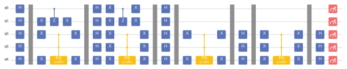
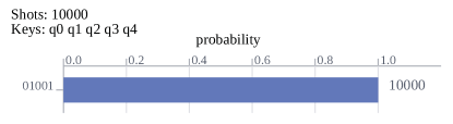
Figure 30: The quantum circuit of the 5-qubit DEGA (target string $\tau=01001$). The parameter in the circuit is $\phi=2\arcsin\left(\sin\left(\frac{\pi}{4J+6}\right)/\sin\theta\right)=2.1268800471555034\approx 2.1269$, where $J=\lfloor(\pi/2-\theta)/(2\theta)\rfloor$ and $\theta=\arcsin{\sqrt{1/2^{3}}}$.

Figure 31: The sampling results of the 5-qubit DEGA (target string $\tau=01001$).

The sampling results demonstrate that $\tau=01001$ is obtained exactly after measurement.

If Grover’s algorithm or the algorithm by Long is employed to search $\tau=01001$, we can build the completed circuits (see Figure 32 and Figure 33) respectively. By sampling the circuits 10,000 times respectively, the results can be found in Figure 35 and Figure 35.

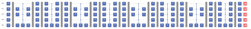
Figure 32: The quantum circuit of the 5-qubit Grover’s algorithm (target string $\tau=01001$).

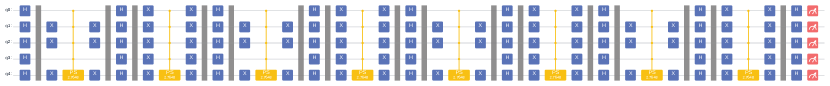
Figure 33: The quantum circuit of the 5-qubit algorithm by Long (target string $\tau=01001$). The parameter in the circuit is $\phi=2\arcsin\left(\sin\left(\frac{\pi}{4J+6}\right)/\sin\theta\right)=2.764763603060391\approx 2.7648$, where $J=\lfloor(\pi/2-\theta)/(2\theta)\rfloor$ and $\theta=\arcsin{\sqrt{1/2^{5}}}$.

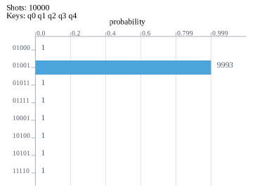
Figure 34: The sampling results of the 5-qubit Grover’s algorithm (target string $\tau=01001$).

Figure 35: The sampling results of the 5-qubit algorithm by Long (target string $\tau=01001$).

The number of quantum gates required by two algorithms is 117, and the circuit depths are 33.

The algorithm by Long and our DEGA can achieve exact search, while Grover’s algorithm can obtain target strings with high probability (see Figure 36).

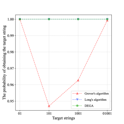
Figure 36: The probability of obtaining the target string by different algorithms.

In addition, the number of quantum gates and circuit depth required by Grover’s and the algorithm by Long are the same, which will be deepened as $n$ increases. However, our DEGA requires fewer quantum gates (see Figure 38) and shallower circuit depth (Figure 38). The circuit depth of our DEGA only depends on the parity of $n$, and it is not deepened as $n$ increases.

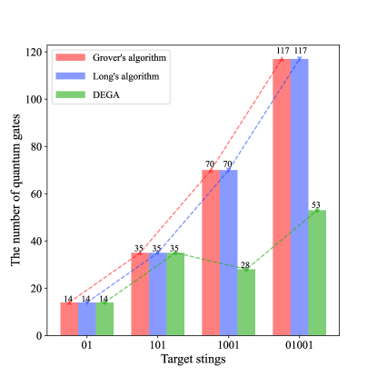
Figure 37: The number of quantum gates required by different algorithms..

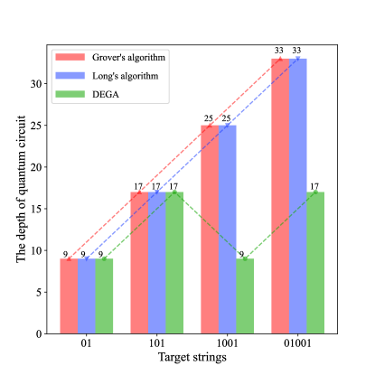
Figure 38: The depth of quantum circuit of different algorithms.

6.8 The depolarization channel

In the above experiment, the quantum circuits we built ignore the influence of noise. However, to run quantum algorithms on real quantum computers, there is a certain error in the operation of each type of quantum gate. In this subsection, we will simulate the 6-qubit DBVA and 5-qubit DEGA running in the depolarization channel that is a crucial type of quantum noise, it further illustrates that distributed quantum algorithm has the superiority of resisting noise.

In the depolarization channel [38], a single qubit will be depolarized with probability $p$. which means it is replaced by complete mixed state $I/2$. Also, it will remain unchanged with the probability of $1-p$. After this noise, the state of the quantum system becomes

$$\varepsilon(\rho)=(1-p)\rho+p\left(\frac{I}{2}\right),$$ (87)

where $\rho$ represents the initial quantum state. For arbitrary state $\rho$, we have

$$\frac{I}{2}=\frac{\rho+X\rho X+Y\rho Y+Z\rho Z}{4},$$ (88)

where $X,Y$ and $Z$ are Pauli operators. Inserting Eq. (88) into Eq. (87) gives

$$\varepsilon(\rho)=\left(1-\frac{3p}{4}\right)\rho+\frac{p}{4}\left(X\rho X+Y\rho Y+Z\rho Z\right).$$ (89)

For convenience, the depolarization channel is sometimes expressed as

$$\varepsilon(\rho)=\left(1-p\right)\rho+\frac{p}{3}\left(X\rho X+Y\rho Y+Z\rho Z\right),$$ (90)

which means the state $\rho$ will remain unchanged with the probability $1-p$, and apply the Pauli operators $X,Y$ or $Z$ with probability $p/3$ for each operators.

Furthermore, the depolarizing channel can be extended to a $d$-dimensional ($d>2$) quantum system. Similarly, the depolarizing channel of a $d$-dimensional quantum system again replaces the quantum system with tcomplete mixed state $I/d$ with probability $p$, and remains unchanged with the probability of $1-p$. The corresponding quantum operation is

$$\varepsilon(\rho)=(1-p)\rho+p\left(\frac{I}{d}\right).$$ (91)

6.8.1 6-qubit DBVA, the hidden string $s=001011$

In this subsection, we simulate the quantum algorithms running in the depolarization channel by adding noise behind each quantum gate. That is, we build the quantum circuits of Figure 12, Figure 13, Figure 16 and Figure 19 in the depolarization channel as shown in Figure 39 to Figure 42. Set the noise parameter $p=0.03$.

Sample the above four circuits in the depolarizing channel 10,000 times, respectively. In order to better reproduce the experimental results, we set the random seeds of simulator and sampling both being 42, the noise parameter $p$ being $0.03$. At last, the results can be found in Figure 46 to Figure 46, respectively.

Figure 39: The quantum circuit of the BV algorithm in the depolarizing channel. Since circuit is too long, divide the whole quantum circuit into upper and lower parts. A gray rectangle represents a barrier gate, which is used to separate quantum gates. And DC represents the depolarization channel.

Figure 40: The quantum circuit of the BV algorithm after optimization in the depolarizing channel.

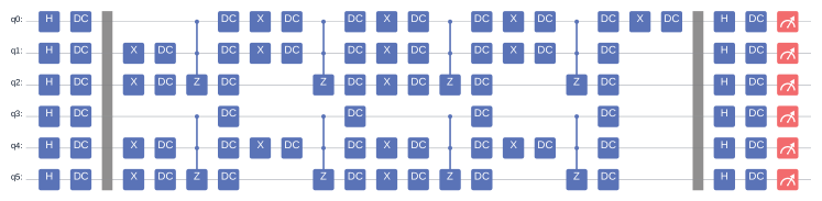
Figure 41: The quantum circuit of DBVA with two computing nodes after optimization in the depolarizing channel.

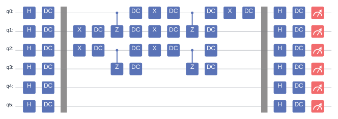
Figure 42: The quantum circuit of DBVA with $t=3$ computing nodes after optimization in the depolarizing channel.

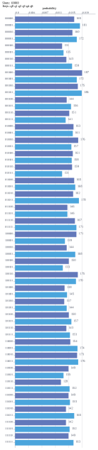
Figure 43: The sampling results of the BV algorithm in the depolarizing channel. The noise parameter $p=0.03$.

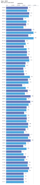
Figure 44: The sampling results of the BV algorithm after optimization in the depolarizing channel. The noise parameter $p=0.03$.

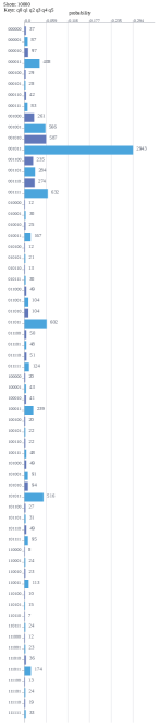
Figure 45: The sampling results of DBVA with two computing nodes after optimization in the depolarizing channel. The noise parameter $p=0.03$.

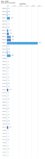
Figure 46: The sampling results of DBVA with $t=3$ computing nodes after optimization in the depolarizing channel. The noise parameter $p=0.03$.

The probability of obtaining the hidden string $s=001011$ are 0.0186, 0.0209, 0.2943 and 0.5611, respectively. However, the desired results were drown out by the channel noise (see Figure 46 and Figure 46). Furthermore, the probability in our DBVA are higher than in the optimized BV algorithm (0.2943 $>$ 0.0209, 0.5611 $>$ 0.0209). When $t$ is greater, the probability is higher (0.5611 $>$ 0.2943).

We already know that there is a certain error in the operation of each type of quantum gate in the depolarizing channel. In other words, the more quantum gates are, the greater the cumulative noise of the quantum circuit is, and the lower the probability of obtaining the target string is. Here, the number of quantum gates required by our DBVA are obviously less than that required by the BV algorithm. At present, to run quantum algorithms on real quantum computers, it is usually necessary to decompose the multi-qubit quantum gates into single-qubit gates and double-qubit gates. If we further consider the decomposition of $C^{n-1}Z$ gates into single-qubit gates and double-qubit gates, the difference between the number of quantum gates required by the BV algorithm and our DBVA will be larger, and the fidelity of theoretical and experimental final states will be lower. However, we will not go into too much details here.

As the number of qubits increases, the depth of quantum circuit or noise parameter $p$ increases, the errors caused by the noise will further accumulate. Fortunately, our DBVA needs fewer quantum gates, resulting in shallower quantum circuits. Hence, our DBVA has higher noise resistance.

6.8.2 5-qubit DEGA, the target string $\tau=01001$

We can rebuild the quantum circuits of the Grover’s algorithm, the algorithm by Long and our DEGA in the depolarization channel (see Figure 47 to Figure 49). Set the noise parameter $p=0.01$ and DC represents the depolarization channel.

Figure 47: The quantum circuit of the 5-qubit Grover’s algorithm (target string $\tau=01001$) in the depolarizing channel.

Figure 48: The quantum circuit of the 5-qubit algorithm by Long (target string $\tau=01001$) in the depolarizing channel. The parameter in the circuit is $\phi=2\arcsin\left(\sin\left(\frac{\pi}{4J+6}\right)/\sin\theta\right)=2.764763603060391\approx 2.7648$, where $J=\lfloor(\pi/2-\theta)/(2\theta)\rfloor$ and $\theta=\arcsin{\sqrt{1/2^{5}}}$.

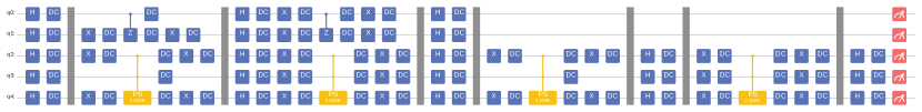
Figure 49: The quantum circuit of the 5-qubit DEGA (target string $\tau=01001$) in the depolarizing channel. The parameter in the circuit is $\phi=2\arcsin\left(\sin\left(\frac{\pi}{4J+6}\right)/\sin\theta\right)=2.1268800471555034\approx 2.1269$, where $J=\lfloor(\pi/2-\theta)/(2\theta)\rfloor$ and $\theta=\arcsin{\sqrt{1/2^{3}}}$.

Sample the above three circuits 10,000 times, respectively. In order to better reproduce the experimental results, we set the random seeds of simulator and sampling both being 42. At last, the sampling results can be found in Figure 52 to Figure 52, respectively. It can be seen that due to the existence of noise, it will not achieve exact search.

Figure 50: The sampling results of 5-qubit Grover’s algorithm in the depolarizing channel. The noise parameter $p=0.01$.

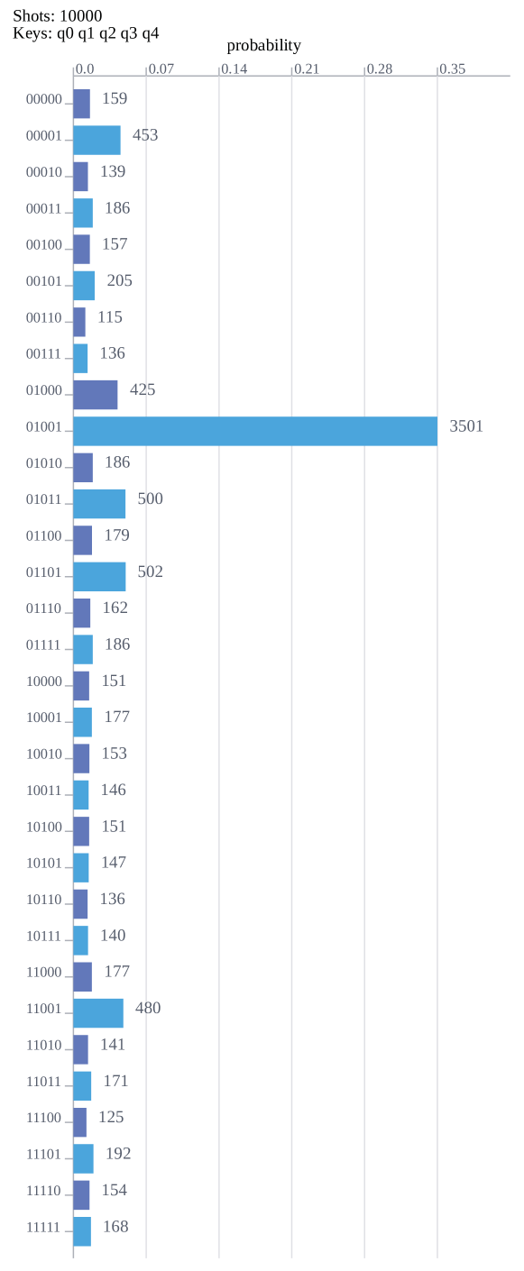
Figure 51: The sampling results of 5-qubit the algorithm by Long in the depolarizing channel. The noise parameter $p=0.01$.

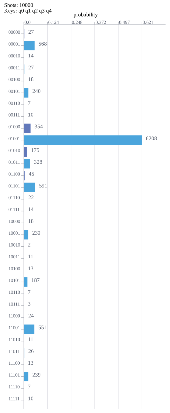
Figure 52: The sampling results of 5-qubit DEGA in the depolarizing channel. The noise parameter $p=0.01$.

Furthermore, we set the noise parameter $p$ as $0,0.01,\cdots,0.09$. The statistical chart as shown in Figure 53.

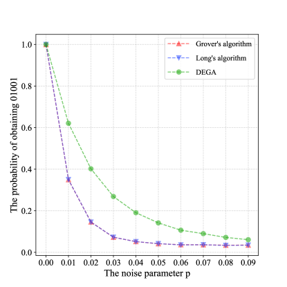
Figure 53: The probability of obtaining $\tau=01001$ by different algorithms.

With the increase of noise parameter $p$, the probability of obtaining $\tau=01001$ decreases. In addition, the probabilities of getting target string by Grover’s algorithm and the algorithm by Long are close. The probability of our DEGA is higher than that of Grover’s algorithm and the algorithm by Long.

When $p=0.07$, the sampling results can be found in Figure 59 to Figure 59, respectively. The desired results are drown out by the channel noise in Grover’s algorithm and the algorithm by Long. However, $\tau=01001$ can still be obtained with a higher probability than other states in our DEGA. Even if $p=0.09$, our DEGA still works (see Figure 59 to Figure 59). It can be found that although the number of qubits of our DEGA is the same as that of Grover’s algorithm and the algorithm by Long, our circuit depth is shallower, so that our scheme is more resistant to the depolarization channel noise.

In short, by simulating the algorithms running in the depolarized channel, it further illustrates that distributed quantum algorithms have the superiority of resisting noise.

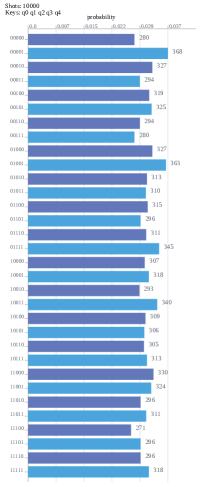
Figure 54: The sampling results of the 5-qubit Grover’s algorithm in the depolarizing channel. The noise parameter $p=0.07$.

Figure 55: The sampling results of the 5-qubit algorithm by Long in the depolarizing channel. The noise parameter $p=0.07$.

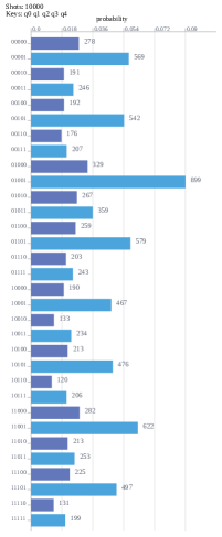
Figure 56: The sampling results of the 5-qubit DEGA in the depolarizing channel. The noise parameter $p=0.07$.

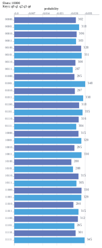
Figure 57: The sampling results of the 5-qubit Grover’s algorithm in the depolarizing channel. The noise parameter $p=0.09$.

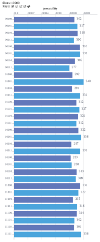
Figure 58: The sampling results of the 5-qubit algorithm by Long in the depolarizing channel. The noise parameter $p=0.09$.

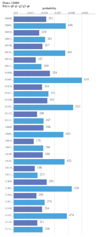
Figure 59: The sampling results of the 5-qubit DEGA in the depolarizing channel. The noise parameter $p=0.09$.

7 Conclusion

Distributed quantum computation has gained extensive attention since small-qubit quantum computers seem to be built more practically in the noisy intermediate-scale quantum (NISQ) era. Hence, researchers are considering how several small-scale devices might collaborate to accomplish a task on a large one.

In this paper, we have given a distributed Bernstein-Vazirani algorithm (DBVA) with $t$ computing nodes, and a distributed exact Grover’s algorithm (DEGA) that solve the search problem with only one target item in the unordered databases. In comparison to the BV algorithm, the circuit depth of DBVA is not greater than $2^{\text{max}(n_{0},n_{1},\cdots,n_{t-1})}+3$ instead of $2^{n}+3$. In addition, the circuit depth of DEGA is $8(n~{}\text{mod}~{}2)+9$, which is less than the circuit depth of Grover’s algorithm, $1+8\left\lfloor\frac{\pi}{4}\sqrt{2^{n}}\right\rfloor$.

Finally, we have provided particular situations of our DBVA and DEGA on MindQuantum to validate the correctness and practicability of our methods. First of all, we have shown how to decompose the original 6-qubit BV problem into two 3-qubit and three 2-qubit tasks. In the next part, we have explicated the specific steps of implementing $n$-qubit DEGA, where $n\in\{2,3,4,5\}$. In the end, we have simulated 6-qubit DBVA and 5-qubit DEGA running in the depolarization channel. By simulating the algorithms running in the depolarized channel, it further illustrates that distributed quantum algorithms have the superiority of resisting noise.

However, we have only designed a distributed exact quantum algorithm for the case of unique target in search problem, so it is still open that designing a distributed exact quantum algorithm solves the search problem with the case of multiple targets.

References

- [1] P. Benioff, The computer as a physical system: a microscopic quantum mechanical Hamiltonian model of computers as represented by Turing machines, Journal of Stat. Phys. 22 (5) (1980) 563-591.
- [2] P. Benioff, Quantum mechanical Hamiltonian models of Turing machines, Journal of Stat. Phys. 29 (3) (1982) 515-546.
- [3] D. Deutsch, Quantum theory, the Church-Turing principle and the universal quantum computer, Proceedings of the Royal Society of London A: Mathematical, Physical and Engineering Sciences 400 (1818) (1985) 97-117.
- [4] D. Deutsch, R. Jozsa, Rapid solution of problems by quantum computation, Proceedings of the Royal Society of London. Series A: Mathematical and Physical Sciences 439 (1907) (1992) 553-558.
- [5] E. Bernstein, U. Vazirani, Quantum complexity theory, Proceedings of the Twenty-Fifth Annual ACM Symposium on Theory of Computing (STOC’93), (1993) pp. 11-20.
- [6] D. R. Simon, On the power of quantum computation, SIAM J. Comput. 26 (5) (1997) 1411-1473.
- [7] P. W. Shor, Algorithms for quantum computation: discrete logarithms and factoring, Proceedings 35th Annual Symposium on Foundations of Computer Science, IEEE, (1994) 124-134.
- [8] L. K. Grover, Quantum mechanics helps in searching for a needle in a haystack, Phys. Rev. Lett. 79 (2) (1997) 325.
- [9] A. W. Harrow, A. Hassidim, S. Lloyd, Quantum algorithm for linear systems of equations, Phys. Rev. Lett. 103 (15) (2009) 150502.
- [10] H. Li, L. Yang, A quantum algorithm for approximating the influences of Boolean functions, Quantum Inf. Process. 14 (6) (2015) 1787-1797.
- [11] Z. Xie, D. Qiu, Quantum algorithms on Walsh transform and Hamming distance for Boolean functions, Quantum Inf. Process. 17 (6) (2018) 139.
- [12] A. Younes, A fast quantum algorithm for the affine Boolean function identification, The Eur. Phys. J. Plus. 130 (2) (2015) 34.
- [13] K. Nagata, G. Resconi, T. Nakamura, and et al., A generalization of the Bernstein-Vazirani algorithm, MOJ Eco Environ. Sci. 2 (1) (2017) 00010-00012.
- [14] D. Christoph, H. Peter, A quantum algorithm for finding the minimum, arXiv: quant-ph/9607014v2, 1996.
- [15] H. Ramesh, V. Vinay, String matching in quantum time, Discrete Algorithms 1 (1) (2003) 103-110.
- [16] A. Ambainis, K. Balodis, J. Iraids, and et al., Quantum speedups for exponential-time dynamic programming algorithms, Proceedings of the 13th Annual ACM-SIAM Symposium on Discrete Algorithms. San Diego: SIAM, (2019) 1783-1793.
- [17] A. Andris, L. Nikita, Quantum algorithms for computational geometry problems, 15th Conference on the Theory of Quantum Computation, Communication and Cryptography, (2020) 9:1-9:10.
- [18] G. Brassard, P. Hoyer, M. Mosca, and et al., Quantum amplitude amplification and estimation, Contemporary Mathematics 305 (2002) 53-74.
- [19] Z. J. Diao, Exactness of the original Grover search algorithm, Phys. Rev. A 82 (4) (2010) 044301.
- [20] G. L. Long, Grover algorithm with zero theoretical failure rate, Phys. Rev. A 64 (2) (2001) 022307.
- [21] J. Preskill, Quantum computing in the NISQ era and beyond, Quantum 2 (2018) 79.
- [22] J. I. Cirac, P. Zoller, Quantum computations with cold trapped ions, Phys. Rev. Lett. 74 (1995) 4091-4094.
- [23] C. Y. Lu, X. Q. Zhou, O. Guhne, and et al., Experimental entanglement of six photons in graph states, Nat. Phys. 3 (2) (2007) 91-95.
- [24] Y. Makhlin, G. Schön, A. Shnirman, Quantum-state engineering with Josephson-junction devices, Rev. Mod.Phys. 73 (2) (2001) 357-400.
- [25] J. Berezovsky, M. H. Mikkelsen, N. G. Stoltz, and et al., Picosecond coherent optical manipulation of a single electron spin in a quantum dot, Science 320 (5874) (2008) 349-352.
- [26] R. Hanson, D. D. Awschalom, Coherent manipulation of single spins in semiconductors, Nature 453 (7198) (2008) 1043-1049.
- [27] S, Endo, Z. Cai, S. C. Benjamin, and et al., Hybrid quantum-classical algorithms and quantum error mitigation, J. Phys. Soc. Jpn. 90 (3) (2021) 032001.
- [28] H. Buhrman and H. Röhrig, Distributed quantum computing, Mathematical Foundations of Computer Science 2003: 28th International Symposium, Springer Berlin Heidelberg, (2003) 1-20.
- [29] A. Yimsiriwattana, S.J. Lomonaco Jr., Distributed quantum computing: a distributed Shor algorithm, Quantum Inf. Comput. II., 5436 (2004) 360.
- [30] R. Beals, S. Brierley, O. Gray and et al., Efficient distributed quantum computing, Proc. R. Soc. A: Math. Phys. Eng. Sci. 469 (2153) (2013) 20120686.
- [31] K. Li, D. W. Qiu, L. Li, and et al., Application of distributed semi-quantum computing model in phase estimation, Inform. Process. Lett. 120 (2017) 23-29.
- [32] J. Avron, O. Casper, and I. Rozen, Quantum advantage and noise reduction in distributed quantum computing, Phys. Rev. A 104 (5) (2021) 052404.
- [33] D. W. Qiu, L. Luo, L. G. Xiao, Distributed Grover’s algorithm, arXiv: 2204.10487v3, 2022.
- [34] J. W. Tan, L. G. Xiao, D. W. Qiu, and et al., Distributed quantum algorithm for Simon’s problem, Phys. Rev. A 106 (3) (2022) 032417.
- [35] L. G. Xiao, D. W. Qiu, L. Luo, and et al., Distributed Shor’s algorithm, Quantum Inf. Comput. 23 (2023) 27-44.
- [36] MindQuantum, https://gitee.com/mindspore/mindquantum, 2021.
- [37] R. Beals, H. Buhrman, R. Cleve, and et al., Quantum lower bounds by polynomials. Proceedings of the 39th Annual Symposium on Foundations of Computer Science, (1998) 352.
- [38] M. A. Nielsen, I. L. Chuang, Quantum Computation and Quantum Information. Cambridge, Cambridge University Press, 2002.