Investigate the strong coupling of $g_{XJ/\psi\phi}$ in $X(4500)\to J/\psi\phi$ by using the three-point sum rules and the light-cone sum rules

Abstract

We assign $X(4500)$ as a D-wave tetraquark state and study the decay of $X(4500)$ $\to$ $J/\psi\phi$. The mass and the decay constant of $X(4500)$ are calculated by using the SVZ sum rules. For the decay width of $X(4500)$ $\to$ $J/\psi\phi$, we present the calculation within the framework of both the three-point sum rules and the light-cone sum rules. The strong coupling $g_{XJ/\psi\phi}$ is obtained by considering the soft-meson approximation when we use the light-cone sum rules calculation. Both calculations show that the decay of $X(4500)$ $\to$ $J/\psi\phi$ close to the total width of $X(4500)$ if we assign $X$(4500) as a D-wave tetraquark. We also consider the open-charm decay channels like $X(4500)\to D_{s}D_{s}$, $X(4500)\to D_{s}^{*}D_{s}$, and $X(4500)\to D_{s}^{*}D_{s}^{*}$ , their widths are small when compared to the width of $X(4500)$, suggesting that the hidden-charm decay channels $X(4500)$ $\to$ $J/\psi\phi$ are predominant when compared with the total width of $X(4500)$. A more rational conclusion can be obtained only if the complete open-charm decay channel is considered. In the future, experiments will be more helpful in determining whether or not this structure of $X(4500)$ is appropriate.

I Introduction

In 2016, the LHCb collaboration analyzed the decay of $B^{+}$ $\to J/\psi\phi K^{+}$ in the $pp$ collision LHCb:2016axx ; LHCb:2016nsl , and found that four resonance-like peaks appeared in the $J/\psi\phi$ invariant mass spectrum. Two of them are named $X(4140)$ and $X(4274)$, and their spin parity numbers are $J^{PC}=1^{++}$. The $J^{PC}$ of the other two, with the names of $X(4500)$ and $X(4700)$ respectively, are $J^{PC}=0^{++}$.

It is necessary to investigate $X(4140)$ and $X(4274)$, $X(4700)$ and $X(4500)$ because they may make up a significant fraction of exotic mesons. Due to the fact that the mass spectrum of $X(4140)$ and $X(4274)$, and the hidden-flavor decay widths of $X(4700)$ have already been calculated with sum rules Agaev:2017foq ; Xie:2022ilz , in this paper, we focus on $X(4500)$, whose mass and width are $\text{M}=4474\pm 3\pm 3\text{MeV}$ and $\Gamma=77\pm 6^{+10}_{-8}\text{MeV}$ respectively LHCb:2021uow .

It is now the structure of X(4500) has not yet been fully established from a variety of studies, that many more works are in progress on this attractive issue.

First, it is interesting to ascertain whether the re-scattering effects may contribute to the resonance peaks in the $J/\psi\phi$ mass spectrum or notLuo:2022xjx . Through investigating this effects or threshold cusps in the process $B^{+}\to J/\psi\phi K^{+}$, the authors in Ref.Liu:2016onn ; Ge:2021sdq found that, for $X$(4700), it can be simulated by the $\psi^{\prime}\phi$ re-scattering via the $\psi^{\prime}K_{1}$ loops, while for $X(4500)$, it is difficult to attribute it to such effects. It may correspond to genuine resonances instead.

Since $X$(4500) appears in the $J/\psi\phi$ invariant mass spectrum, we could speculate that it can be a charmonium. Whether $X(4500)$ is assigned as a $4^{3}P_{0}$ state in the constituent quark model Fernandez:2016bqr ; Ortega:2016hde or assigned as a $\chi_{c0}(4P)$ state in the linear potential modelGui:2018rvv , its predicted mass and width are consistent within the experimental uncertainties. The theoretical calculation shows that $4^{3}P_{0}$ will dominantly decay into charm mesons like $DD_{1}$, $DD_{1}^{\prime}$, $D^{*}D^{\prime}$, and $D^{*}D^{*}_{2}$, and that $\chi_{c0}(4P)$ will dominantly decay into $DD_{1}$, $DD_{1}^{\prime}$, $D^{*}D_{0}$, $D^{*}D_{2}$. However, in experiemnt, no relevant signal of $X(4500)$ appears in the $B\to$ $D^{(*)}_{(s)}\bar{D}^{*}_{(s)}K$ decays Olsen:2017bmm . Besides, since $\chi_{cJ}(nP)$ $\to$ $J/\psi\omega$ is similar to $X(4500)\to J/\psi\phi$, we can surmise the $J/\psi\omega$ mass spectrum in $B^{+}$ $\to J/\psi\omega K^{+}$ decay should appear some structures resembling the $J/\psi\phi$ mass peaks. But this was rejected by experiment BaBar:2012nxg ; Belle:2009and , which contradicts a charmonium interpretation for the $X(4500)$. In addition, in the screened potential model Gui:2018rvv , $\chi_{c0}(5P)$ is a good candidate for $X$(4500), since its predicted mass is $4537$ MeV. Whereas, the total width of $\chi_{c0}(5P)$ is about $15$ MeV, 4 times smaller than that of $X$(4500) observed in the experiment.

Although $X(4500)$ is inconsistent with pure charmonium, it could be $J/\psi-\phi$ or $\Psi(2S)-\phi$ bound state since it appears in the spectrum of $J/\psi\phi$. Unfortunately, lattice QCD exhibited weak attraction of $J/\psi-\phi$ at low energies Ozaki:2012ce , and $\Psi(2S)-\phi$ bound state description has already been occupied by $X(4274)$ Panteleeva:2018ijz . In some specific parameter space, $X(4500)$ might be assigned as other hadrocharmonium states but require different binding mechanisms Panteleeva:2018ijz . It can also be expanded as hybrid state which is a charmonium state that incorporates excited gluon fields. For example, the mass of $X(4500)$ is compatable with that of $0^{++}$ hybrid $1p_{0}(H_{3})$ state in the NRQCD results Oncala:2017hop . But it’s tricky to expalin $X(4500)$ observed in $J/\psi\phi$ channel, since $1p_{0}(H_{3})$ only contains small pieces of charmonium.

In addition to these charmonium-related explanations, some theoretical studies are oriented toward the $cs\bar{c}\bar{s}$ tetraquark state.

Reported by Maiani et al.Maiani:2016wlq , $X(4500)$ can be assigned as radial excitations of $X(4140)$ while $X(4140)$ was arranged as a $cs\bar{c}\bar{s}$ ground state. Similarly, in Ref.Lu:2016cwr , it was regarded as a tetraquark that incorporates one 2S scalar diquark and one scalar antidiquark within the relativized quark model. In other models like the diquark-antidiquark model Zhu:2016arf , $X(4500)$ was explained as a radial excitation of $J^{P}=0^{+}$ tetraquark with quark content $\frac{1}{\sqrt{3}}(u\bar{u}+d\bar{d}+s\bar{s})c\bar{c}$, and in the chiral quark model Yang:2019dxd , it was explained as a 2S radial excited compact tetraquark state with $J^{PC}=0^{++}$. Besides, as illustrated in the color flux-tube model with a multibody confinement potential Deng:2017xlb , $X(4500)$ can be probably considered as a $0^{++}$ compact tetraquark states $cs\bar{c}\bar{s}$ although its mass is slightly higher than $4500$ MeV. In the framework of the quark delocalization color screening model Liu:2021xje , $X(4500)$ has been assigned as a $IJ^{P}=00^{+}$ compact tetraquark resonance state, or a radial excitions of S-wave scalar diquark-antidiquark bound states with quantum number $0^{++}$ in the diquark model Anwar:2018sol . Moreover, in the sum rules approach Reinders:1984sr , it can also be considered as a first radial excited state Wang:2016gxp or a D-wave $cs\bar{c}\bar{s}$ tetraquark states Chen:2016oma .

As we mentioned, with the method of SVZ sum rules, $X$(4500) has been investigated in Ref.Chen:2016oma in which its mass is predicted. Because of the deficiency of hidden-charm decay width and open-charm decays width, we consider the hidden-charm decay and open-charm decay channel in this article. Following the assumption in the Ref.Chen:2016oma , we consider $X$(4500) a D-wave tetraquark state in our study. When we assign $X(4500)$ as a D-wave tetraquark, $X(4500)$ can possibly decay into $D_{s}D_{s}$, $D_{s}^{*}D_{s}$, and $D_{s}^{*}D_{s}^{*}$. Furthermore, by performing the Fierz and color rearrangements on the currents and changing it to mesonic-mesonic structures, the decay channels associated with $X(4500)$ can be obtainedChen:2016qju ; Chen:2006hy ; Chen:2007xr . We can list the final state as follows: to be S-wave $D^{*}_{s}D^{*}_{s1}(2860)$, $D^{*}_{s}D^{*}_{s3}(2860)$, P-wave $D^{*}_{s}D^{*}_{s0}$, $D^{*}_{s}D_{s1}$, $D^{*}_{s}D^{*}_{s2}$ , and D-wave $D_{s}^{*}D_{s}^{*}$ and etc. Since only the D meson light cone distribution amplitude (LCDA) is well defined in Refs Zuo:2006re ; Li:2008ts , there is no systematic development of the D family meson LCDAs in the literature, so we deal with some open-charm decays like $D_{s}D_{s}$, $D_{s}^{*}D_{s}$, and $D_{s}^{*}D_{s}^{*}$ with three-point sum rule. Some other decays involving $D_{sJ}^{*},J=0,1,2$ are much more troublesome because $D_{sJ}^{*},J=0,1,2$ structures are complicated and unstable. Therefore, the only open-charm decay channels we consider in this paper are the $X(4500)\to D_{s}D_{s}$, $X(4500)\to D_{s}^{*}D_{s}$, and $X(4500)\to D_{s}^{*}D_{s}^{*}$ . We calculate the mass of $X(4500)$ by conducting the dimension regulation in SVZ sum rules at first, and obtain the results comparable with those in PDG ParticleDataGroup:2020ssz . We then evaluate its decay constant which is used in the numerical calculation of the strong coupling $g_{XJ/\psi\phi}$. Typically, we calculate $g_{XJ/\psi\phi}$ through both the three-point sum rules and the light-cone sum rules (LCSR) methods simultaneously. According to our calculations, different methods have congruent decay widths of $X\text{(4500)}\to$ $J/\psi\phi$. We compared the results with the total widths of $X$(4500) with the experiment and demonstrate some valuable discussions. The results are instructive for future experiments to further determine the structure of $X(4500)$. To previous works on $X$(4500) Chen:2016oma , our study can be perceived as a supplement.

The structure of the paper is arranged as follows. In Section.II, the strong coupling $g_{XJ/\psi\phi}$ is obtained by using both the three-point sum rules and the light-cone sum rules. Through the two-point SVZ sum rules, we study the mass and decay constant of $X$(4500). The numerical results and discussions are provided in Section.III. We come to the summary in Section.IV.

II Calculation Framework

II.1 The mass and the decay constant of $X(4500)$

In this section, we calculate the mass and the decay constant of $X(4500)$ to extract their values. The two-point function provides the foundation for the sum rule calculation of the mass:

$$\Pi^{\text{SVZ}}(p)=i\int\mbox{d}^{4}xe^{ipx}\braket{0}{T\{J^{X}(x)J^{X\dagger}(0)\}}{0},$$ (1)

The interpolating currents of $X(4500)$ is given byChen:2016oma :

$$J^{X}(x) =c_{k}^{T}(x)C\gamma_{\mu 1}[\overrightarrow{D}_{\mu 3}\overrightarrow{D}_{\mu 4}s_{l}(x)]$$

$$\quad(\bar{c}_{k}(x)\gamma_{\mu 2}Cs_{l}^{T}(x)-\bar{c}_{l}(x)\gamma_{\mu 2}C\bar{s}_{k}^{T}(x))$$

$$\times(g^{\mu 1\mu 3}g^{\mu 2\mu 4}+g^{\mu 1\mu 4}g^{\mu 2\mu 3}-g^{\mu 1\mu 2}g^{\mu 3\mu 4}/2),$$

where $\overrightarrow{D}_{\mu}=\overrightarrow{\partial}_{\mu}+igT^{j}A_{\mu}^{j}$. The subscripts $s,c$ refer to the strange and charm quarks, and the subscripts $j$, $k$, $l$ to the color indices, and $C$ for the charge conjugation matrix.

A phenomenological expression of the correlation function can be given by considering the complete set of hadronic states:

$$\Pi^{\text{SVZ,phen}}(p)=$$ (2)

$$\frac{\braket{0}{J^{X}}{X(p)}\braket{X(p)}{J^{X\dagger}}{0}}{m_{X}^{2}-p^{2}}+\int_{s^{\prime}}^{\infty}d\hat{s}\frac{\tilde{\rho}^{\text{SVZ,phen}}(\hat{s})}{\hat{s}-p^{2}},$$

Here the higher resonances and continuum states are referred to as $\tilde{\rho}^{\text{SVZ,phen}}$. Since the subtraction terms will vanish after Borel transformation, they are not shown here.

Next, by replacing all matrix elements with

$$\braket{0}{J^{X}}{X(p^{\prime})}=m_{X}f_{X}$$ (3)

and performing the Borel transformation, the Eq.(2) can be written as

$$\Pi^{\text{SVZ,phen}}(M^{2})=$$ (5)

$$(m_{X})^{2}(f_{X})^{2}e^{-(m_{X})^{2}/M^{2}}+\int_{s^{\prime}}^{\infty}d\hat{s}\tilde{\rho}^{\text{SVZ,phen}}(\hat{s})e^{-\hat{s}/M^{2}}.$$

Now we’ll establish the correlation function on the OPE side, where the non-vanishing vacuum expectation of quark and gloun condensate such as $\langle\bar{q}q\rangle$,$\langle\bar{q}g_{s}\sigma Gq\rangle$ are introduced. First, we express the correlation function with interpolating currents in Eq.(II.1), perform the Wick Theorem, then the correlation function can be recast to be

$$\Pi^{\text{SVZ,OPE}}(p)=i\int\mbox{d}^{4}xe^{ipx}$$ (6)

$$\text{Tr}[\gamma_{\mu 1}(\overrightarrow{D}_{\mu 3}\overrightarrow{D}_{\mu 4}S^{kk^{\prime}}_{s}(x-y)\overleftarrow{D}_{\nu 3}\overleftarrow{D}_{\nu 4})\gamma_{\nu 1}\gamma_{5}\tilde{S}_{c}^{jj^{\prime}}(-x)]|_{y=0}$$

$$(\text{Tr}[\gamma_{\mu 2}\tilde{S}^{kk^{\prime}}_{s}(-x)\gamma_{\nu 2}S_{c}^{jj^{\prime}}(-x)]$$

$$-\text{Tr}[\gamma_{\mu 2}\tilde{S}^{kj^{\prime}}_{s}(-x)\gamma_{\nu 2}S_{c}^{jk^{\prime}}(-x)]$$

$$-\text{Tr}[\gamma_{\mu 2}\tilde{S}^{jk^{\prime}}_{s}(-x)\gamma_{\nu 2}S_{c}^{kj^{\prime}}(-x)]$$

$$+\text{Tr}[\gamma_{\mu 2}\tilde{S}^{jj^{\prime}}_{s}(-x)\gamma_{\nu 2}S_{c}^{jj^{\prime}}(-x)])$$

$$\times (g^{\mu 1\mu 3}g^{\mu 2\mu 4}+g^{\mu 1\mu 4}g^{\mu 2\mu 3}-g^{\mu 1\mu 2}g^{\mu 3\mu 4}/2)$$

$$\times (g^{\nu 1\nu 3}g^{\nu 2\nu 4}+g^{\nu 1\nu 4}g^{\nu 2\nu 3}-g^{\nu 1\nu 2}g^{\nu 3\nu 4}/2).$$

In this case, one must deal with divergences in the double integrals like:

$$\int\frac{d^{4}x}{x^{2n}}\int\int\frac{d^{4}k_{1}d^{4}k_{2}e^{ipx-ik_{1}x-ik_{2}x}}{(k_{1}^{2}-m_{c}^{2})(k_{2}^{2}-m_{c}^{2})}.$$ (7)

what we have to do is transform the coordinate to the momentum space in D-dimensio by the Fourier transformationAgaev:2016dev

$$\begin{aligned} &\frac{1}{\left(x^{2}\right)^{n}}=\int\frac{d^{D}p}{(2\pi)^{D}}e^{-ip\cdot x}i(-1)^{n+1}2^{D-2n}\pi^{D/2}\\ &\times\frac{\Gamma(D/2-n)}{\Gamma(n)}\left(-\frac{1}{p^{2}}\right)^{D/2-n}\end{aligned}$$ (8)

The results combine the with remains part dimensionally regularize at D = 4 Matheus:2006xi . Then we can extract the spectral densitythe form imaginary part of results.

The OPE side of the correlation function also can be written as:

$$\Pi^{\text{SVZ,OPE}}(p)=\int_{4m_{c}^{2}}^{\infty}\mbox{d}\hat{s}\frac{\tilde{\rho}^{\text{SVZ,OPE}}(\hat{s})}{\hat{s}-p^{2}},$$ (9)

where $\tilde{\rho}^{\text{SVZ,OPE}}(\hat{s})$ corresponds to the spectral density.

By performing the Borel transform at both the Eq.(2) and Eq.(9), equating the obtained expression:

$$\int_{4m_{c}^{2}}^{\infty}\mbox{d}\hat{s}\tilde{\rho}^{\text{SVZ,OPE}}(\hat{s})e^{-\hat{s}/M^{2}}=$$ (10)

$$(m_{X})^{2}(f_{X})^{2}e^{-(m_{X})^{2}/M^{2}}+\int_{s_{0}}^{\infty}\tilde{\rho}^{\text{SVZ,OPE}}(\hat{s})e^{-\hat{s}/M^{2}},$$

and subtracting the continuum contribution, we find the expression:

$$(m_{X})^{2}(f_{X})^{2}e^{-(m_{X})^{2}/M^{2}}=\int_{4m_{c}^{2}}^{s_{0}}\mbox{d}\hat{s}\tilde{\rho}^{\text{SVZ.OPE}}(\hat{s})e^{-\hat{s}/M^{2}}.$$ (11)

Finally the mass of the state $X(4500)$ can be obtained as

$$(m_{X})^{2}=\frac{\int_{4m_{c}^{2}}^{s_{0}}\mbox{d}\hat{s}\hat{s}\tilde{\rho}^{\text{SVZ,OPE}}(\hat{s})e^{-\hat{s}/M^{2}}}{\int_{4m_{c}^{2}}^{s_{0}}\mbox{d}\hat{s}\tilde{\rho}^{\text{SVZ,OPE}}(\hat{s})e^{-\hat{s}/M^{2}}}.$$ (12)

In Appendix V.3, we provide the spectral densities for $J^{X}$.

II.2 The strong coupling $g_{XD_{S}D_{S}}$, $g_{XD_{S}D_{S}^{*}}$, $g_{XD_{S}^{*}D_{S}^{*}}$ in the three-point sum rules

The QCD sum rulesReinders:1984sr allows us to describe the strong interaction at the low energy level. We are going to consider $X$(4500) as a D-wave tetraquark state and predict the decay width of $X(4500)$ $\to$ $D_{s}D_{s}$, $X(4500)$ $\to$ $D_{s}D_{s}^{*}$ and $X(4500)$ $\to$ $D_{s}^{*}D_{s}^{*}$. The starting point of sum rules is to write down the T-ordered product of three currents for the correlation function:

$$\Pi^{\text{DD}}\left(p^{\prime},p,q\right)$$

$$= \int d^{4}xd^{4}ye^{ip\cdot x}e^{iq\cdot y}\left\langle 0\left|T\left[J^{D_{s}}(x)J^{D_{s}\dagger}(y)J^{X\dagger}(0)\right]\right|0\right\rangle,$$

$$\Pi^{\text{DDs}}\left(p^{\prime},p,q\right)$$

$$= \int d^{4}xd^{4}ye^{ip\cdot x}e^{iq\cdot y}\left\langle 0\left|T\left[J^{D_{s}}_{\mu}(x)J^{D_{s}^{*}\dagger}(y)J^{X\dagger}(0)\right]\right|0\right\rangle,$$

$$\Pi_{\mu\nu}^{\text{DsDs}}\left(p^{\prime},p,q\right)$$

$$= \int d^{4}xd^{4}ye^{ip\cdot x}e^{iq\cdot y}\left\langle 0\left|T\left[J^{D_{s}^{*}}_{\mu}(x)J^{D_{s}^{*}\dagger}_{\nu}(y)J^{X\dagger}(0)\right]\right|0\right\rangle,$$

where $p$, $q$ represent the four-momentum of two final state respectively. Momentum conservation dictates that $X(4500)$ has the four-momentum of $p^{\prime}=p+q$. Meanwhile the interpolating currents for $J^{D_{s}}$,$J^{D_{s}^{*}}_{\mu}$ are given byBracco:2006xf :

$$J^{D_{s}}=i\bar{c}_{a}\gamma_{5}s_{a},\ J^{D_{s}^{*}}_{\mu}=\bar{c}_{b}\gamma_{\mu}s_{b}.$$ (16)

where the subscripts $a$, $b$ refer to the color indices.

Next, in an attempt to evaluate the phenomenological side of the correlation function(II.2), (II.2) and (II.2). we insert intermediate states for $X(4500)$, $D_{s}$, $D_{s}^{*}$ into Eq(II.2), (II.2) and (II.2) and write down the correlation function as

$$\Pi_{\mu\nu}^{\text{DsDs}}\left(p^{\prime},p,q\right)$$ (17)

$$= g_{XD_{s}^{*}D_{s}^{*}}g_{\mu^{\prime}\nu^{\prime}}\left(g_{\mu\mu^{\prime}}-\frac{p_{\mu}p_{\mu^{\prime}}}{m_{D_{s}^{*}}^{2}}\right)\left(g_{\nu\nu^{\prime}}-\frac{p_{\nu}p_{\nu^{\prime}}}{m_{X}^{2}}\right)\times$$

$$\frac{f_{D_{s}^{*}}^{2}f_{X}}{\left(p^{\prime 2}-m_{X}^{2}+i\epsilon\right)\left(p^{2}-m_{D_{s}^{*}}^{2}+i\epsilon\right)\left(q^{2}-m_{D_{s}^{*}}^{2}+i\epsilon\right)}$$

$$+\ldots$$

$$= \frac{g_{XD_{s}^{*}D_{s}^{*}}f_{D_{s}^{*}}^{2}f_{X}}{\left(p^{\prime 2}-m_{X}^{2}+i\epsilon\right)\left(p^{2}-m_{D_{s}^{*}}^{2}+i\epsilon\right)\left(q^{2}-m_{D_{s}^{*}}^{2}+i\epsilon\right)}\times$$

$$\left(g_{\mu\nu}-\frac{p^{\prime}_{\mu}p_{\nu}+p^{\prime}_{\mu}p^{\prime}_{\nu}}{m_{X}^{2}}-\frac{p_{\mu}p_{\nu}}{m_{D_{s}^{*}}^{2}}+\frac{p^{\prime}\cdot p\left(p_{\mu}p_{\nu}+p^{\prime}_{\nu}p_{\mu}\right)}{m_{X}^{2}m_{D_{s}^{*}}^{2}}\right)$$

$$+\ldots.$$

$$\Pi_{\mu\nu}^{\text{DD}}\left(p^{\prime},p,q\right)$$

$$= \frac{-g_{XD_{s}D_{s}}f_{D_{s}}^{2}f_{X}m_{D_{s}}^{4}}{(m_{c}+m_{s})^{2}\left(p^{\prime 2}-m_{X}^{2}+i\epsilon\right)\left(p^{2}-m_{D_{s}}^{2}+i\epsilon\right)\left(q^{2}-m_{D_{s}}^{2}+i\epsilon\right)}$$

$$+\ldots.$$

$$\Pi_{\mu\nu}^{\text{DDs}}\left(p^{\prime},p,q\right)$$

$$= \frac{ig_{XD_{s}^{*}D_{s}}f_{D_{s}^{*}}f_{D_{s}}m_{D_{s}}^{2}m_{D_{s}^{*}}f_{X}}{(m_{c}+m_{s})\left(p^{\prime 2}-m_{X}^{2}+i\epsilon\right)\left(p^{2}-m_{D_{s}^{*}}^{2}+i\epsilon\right)\left(q^{2}-m_{D_{s}}^{2}+i\epsilon\right)}$$

$$\times(-q^{\mu}+\frac{p\cdot q}{m_{D_{s}^{*}}^{2}}p_{\mu})+\ldots.$$

Here $\dots$ denotes all the higher excited state contributions. In order to establish Eq.(17), we have used the relationshipsBracco:2006xf :

$$\braket{0}{J^{X}}{X(p^{\prime})}=m_{X}f_{X}$$

$$\braket{0}{J^{D_{s}}}{D(p)}=\frac{m_{D_{s}}^{2}}{m_{c}+m_{s}}f_{D_{s}}$$

$$\braket{0}{J_{\mu}^{D_{s}^{*}}}{D_{s}^{*}(p)}=m_{D_{s}^{*}}f_{D^{*}_{s}}\varepsilon_{\mu},$$ (18)

in which $\epsilon_{\mu}$ is the polarization vector of $\phi$ and $J/\psi$. $f_{D_{s}(X,D_{s}^{*})}$ is the decay constant of $D_{s}(X(4500),D_{s}^{*})$. Besides, the coupling constant $g_{XD_{s}^{*}D_{s}^{*}}$ came from the matrix element $\langle\phi(q)J/\psi(p)|X(p^{\prime})\rangle$:

$$\langle D_{s}^{*}(q)D_{s}^{*}(p)| X(p^{\prime})\rangle$$ (19)

$$= g_{XD_{s}^{*}D_{s}^{*}}[(q\cdot\varepsilon^{*})(p\cdot\varepsilon^{\prime})-(q\cdot p)(\varepsilon^{*}\cdot\varepsilon^{\prime})].$$

$$\langle D_{s}(q)D_{s}(p)| X(p^{\prime})\rangle=g_{XD_{s}D_{s}}.$$

$$\langle D_{s}(q)D_{s}^{*}(p)| X(p^{\prime})\rangle=g_{XD_{s}D_{s}^{*}}q\cdot\varepsilon.$$

After entering the currents into (II.2), (II.2) and (II.2) and applying the Wick Theorem, the OPE side of the sum rules is:

$$\Pi_{\mu\nu}^{\text{DD,OPE}}\left(p^{\prime},p,q\right)=\int d^{4}xd^{4}ye^{ip\cdot x}e^{iq\cdot y}$$

$$\{\text{Tr}[S^{al}_{c}(-x)\gamma_{5}S^{ak}_{s}(y-z)\overleftarrow{D}_{\mu 3}\overleftarrow{D}_{\mu 4}$$

$$~{}~{}~{}~{}~{}~{}\gamma_{\nu 1}\tilde{S}^{bl}_{c}(-y)\gamma_{5}\tilde{S}^{bk}_{s}(y)\gamma_{\mu 2}]$$

$$-\text{Tr}[S^{ak}_{c}(-x)\gamma_{5}S^{ak}_{s}(y-z)\overleftarrow{D}_{\mu 3}\overleftarrow{D}_{\mu 4}$$

$$~{}~{}~{}~{}~{}~{}\gamma_{\nu 1}\tilde{S}^{bl}_{c}(-y)\gamma_{5}\tilde{S}^{bl}_{s}(y)\gamma_{\mu 2}]\},$$ (20)

$$\Pi_{\mu\nu}^{\text{DsD,OPE}}\left(p^{\prime},p,q\right)=\int d^{4}xd^{4}ye^{ip\cdot x}e^{iq\cdot y}$$

$$\{\text{Tr}[S^{al}_{c}(-x)\gamma_{\mu}S^{ak}_{s}(y-z)\overleftarrow{D}_{\mu 3}\overleftarrow{D}_{\mu 4}$$

$$~{}~{}~{}~{}~{}~{}\gamma_{\nu 1}\tilde{S}^{bl}_{c}(-y)\gamma_{5}\tilde{S}^{bk}_{s}(y)\gamma_{\mu 2}]$$

$$-\text{Tr}[S^{ak}_{c}(-x)\gamma_{\mu}S^{ak}_{s}(y-z)\overleftarrow{D}_{\mu 3}\overleftarrow{D}_{\mu 4}$$

$$~{}~{}~{}~{}~{}~{}\gamma_{\nu 1}\tilde{S}^{bl}_{c}(-y)\gamma_{5}\tilde{S}^{bl}_{s}(y)\gamma_{\mu 2}]\},$$ (21)

$$\Pi_{\mu\nu}^{\text{DsDs,OPE}}\left(p^{\prime},p,q\right)=\int d^{4}xd^{4}ye^{ip\cdot x}e^{iq\cdot y}$$

$$\{\text{Tr}[S^{al}_{c}(-x)\gamma_{\mu}S^{ak}_{s}(y-z)\overleftarrow{D}_{\mu 3}\overleftarrow{D}_{\mu 4}$$

$$~{}~{}~{}~{}~{}~{}\gamma_{\nu 1}\tilde{S}^{bl}_{c}(-y)\gamma_{\nu}\tilde{S}^{bk}_{s}(y)\gamma_{\mu 2}]$$

$$-\text{Tr}[S^{ak}_{c}(-x)\gamma_{\mu}S^{ak}_{s}(y-z)\overleftarrow{D}_{\mu 3}\overleftarrow{D}_{\mu 4}$$

$$~{}~{}~{}~{}~{}~{}\gamma_{\nu 1}\tilde{S}^{bl}_{c}(-y)\gamma_{\nu}\tilde{S}^{bl}_{s}(y)\gamma_{\mu 2}]\},$$ (22)

where we have denoted

$$\tilde{S}_{q}^{ab}(x)=CS_{q}^{ab}(x)C,$$ (23)

and $S_{q}^{ab}(x)$ are the quark ($q=s,c$) propagators. For the light quark ($q=s$), propagators are expressed in terms of Huang:2010dc ; Agaev:2016mjb

$$S_{q}^{ab}(x) = \frac{i\delta_{ab}\not{x}}{2\pi^{2}x^{4}}-\frac{\delta_{ab}m_{q}}{4\pi^{2}x^{2}}-\frac{{\langle\bar{q}q\rangle}}{12}$$ (24)

$$-\frac{i}{32\pi^{2}}\frac{\lambda^{e}}{2}g_{s}G_{\mu\nu}^{e}\frac{1}{x^{2}}(\sigma^{\mu\nu}\not{x}+\not{x}\sigma^{\mu\nu})$$

$$+\frac{i\delta_{ab}\not{x}m_{q}{\langle\bar{q}q\rangle}}{48}-\frac{\delta_{ab}{\langle\bar{q}g_{s}\sigma Gq\rangle}x^{2}}{192}$$

$$+\frac{i\delta_{ab}x^{2}\not{x}m_{q}\langle\bar{q}g_{s}\sigma Gq\rangle}{1152}$$

$$-\frac{i\delta_{ab}x^{2}\not{x}g_{s}^{2}\langle\bar{q}q\rangle^{2}}{7776}-\frac{\delta_{ab}x^{4}\langle\bar{q}q\rangle\langle g_{s}^{2}GG\rangle}{27648},\quad\quad$$

here $e$ is the color index, and the heavy quark ($q=c$) propagator is given by Reinders:1984sr ; Yang:2020wkh

$$S_{q}^{ab}(x) = i\int\frac{d^{4}k}{(2\pi)^{4}}e^{-ikx}\left\{\frac{\delta_{ab}\left(k+m_{q}\right)}{k^{2}-m_{q}^{2}}\right.$$ (25)

$$\left.-\frac{g_{s}G^{ab}_{\mu\nu}}{4}\frac{\sigma_{\mu\nu}\left(k+m_{q}\right)+\left(k+m_{q}\right)\sigma_{\mu\nu}}{\left(k^{2}-m_{q}^{2}\right)^{2}}\right.$$

$$\left.+\frac{g_{s}^{2}G^{2}}{12}\delta_{ab}m_{q}\frac{k^{2}+m_{q}k}{\left(k^{2}-m_{q}^{2}\right)^{4}}+\cdots\right\}.$$

Here we indicate that

$$G^{ab}_{\mu\nu}\equiv G^{f}_{\mu\nu}t_{ab}^{f},\quad G^{2}=G_{\mu\nu}^{f}G^{f\mu\nu}.$$ (26)

where $f$ denote the color index.

As we see, in the phenomenological side expressed in Eq.(II.2),Eq.(17), there emerge several structures like $g_{\mu\nu}$, $p_{\mu}p_{\nu}$ and so on. We consider the $g_{\mu\nu}$ and $q_{\mu}$ structure in Eq.(II.2), Eq.(17) respectively, and make a Borel transform with respect to $-p^{2}=-q^{2}\to M^{2}$ on both the phenomenological and the OPE sides to get the coupling constantDias:2013xfa : Hence, we derive:

$$A(\frac{4m_{D_{s}^{*}}^{2}-m_{X}^{2}}{M^{2}}e^{\frac{m_{D_{s}^{*}}^{2}}{M^{2}}}-4e^{\frac{m_{D_{s}^{*}}^{2}}{M^{2}}}+4e^{\frac{m_{X}^{2}}{4M^{2}}})+Be^{-\hat{s}_{0}/M^{2}}$$

$$=\Pi_{1}^{DsDs}(M^{2})+\Pi_{2}^{DsDs}(M^{2})$$ (27)

$$C(\frac{4m_{D_{s}}^{2}-m_{X}^{2}}{M^{2}}e^{\frac{m_{D_{s}}^{2}}{M^{2}}}-4e^{\frac{m_{D_{s}}^{2}}{M^{2}}}+4e^{\frac{m_{X}^{2}}{4M^{2}}})+De^{-\hat{s}_{0}/M^{2}}$$

$$=\Pi_{1}^{DD}(M^{2})+\Pi_{2}^{DD}(M^{2})$$ (28)

$$E(\frac{4m_{D_{s}^{*}}^{2}-m_{X}^{2}}{M^{2}}e^{\frac{m_{D_{s}^{*}}^{2}}{M^{2}}}-4e^{\frac{m_{D_{s}^{*}}^{2}}{M^{2}}}+4e^{\frac{m_{X}^{2}}{4M^{2}}})+Fe^{-\hat{s}_{0}/M^{2}}$$

$$=\Pi_{1}^{DDs}(M^{2})+\Pi_{2}^{DDs}(M^{2})$$ (29)

where $\hat{s}_{0}$ is the continuum threshold parameter for $X(4500)$,

$$A=\frac{g_{XD_{s}^{*}D_{s}^{*}}f_{D_{s}^{*}}^{2}f_{X}}{(4m_{D_{s}^{*}}^{2}-m_{X}^{2})^{2}},C=\frac{g_{XD_{s}D_{s}}f_{D_{s}}^{2}f_{X}m_{D_{s}}^{4}}{(m_{c}+m_{s})^{2}(4m_{D_{s}}^{2}-m_{X}^{2})^{2}}$$

$$E=\frac{g_{XD_{s}D_{s}^{*}}f_{D_{s}^{*}}f_{D_{s}}f_{X}m_{D_{s}}^{2}m_{D_{s}^{*}}}{(m_{c}+m_{s})(4m_{D_{s}^{*}}^{2}-m_{X}^{2})^{2}}$$ (30)

and $B,D,F$ are the parameters introduced to take into account single pole contributions associated with pole-continuum transitions in a three-point function sum rule Navarra:2006nd ; Colangelo:1994es ; Colangelo:1994es ; Ioffe:1983ju . We show the details of $\Pi_{1}(M^{2}),\Pi_{2}(M^{2})$ in Appendix V.1.

To determine the coupling constant $g_{XD_{s}^{*}D_{s}^{*}}$ we can fit the results with the analytical expression in the left-hand side with right-hand side of Eq.(II.2) to find the value of A. Using the definition of A in Eq.(II.2), we can obtain the values of coupling constants.

Finally, the decay width of $X(4500)$ $\to$ $AB$ can be calculated by equation Dias:2013xfa

$$\Gamma(X(4500)\to AB)=\frac{(g_{XAB})^{2}}{24\pi m_{X}^{2}}$$ (31)

$$\times \lambda(m_{X},m_{A},m_{B})\left(3+\frac{\lambda(m_{X},m_{A},m_{B})}{m^{2}_{A}}\right),\quad$$

where

$$\lambda(a,b,c)=\frac{\sqrt{a^{4}+b^{4}+c^{4}-2(a^{2}b^{2}+b^{2}c^{2}+c^{2}a^{2})}}{2a}.$$ (32)

II.3 The strong coupling $g_{XJ/\psi\phi}$ in the three-point sum rules

Next, we are going to predict the decay width of $X(4500)$ $\to$ $J/\psi\phi$. We need to calculate the strong coupling $g_{XJ/\psi\phi}$ in the first place. The starting point is to write down the correlation function:

$$\Pi_{\mu\nu}^{\text{TP,Hidden}}\left(p^{\prime},p,q\right)$$

$$= \int d^{4}xd^{4}ye^{ip\cdot x}e^{iq\cdot y}\left\langle 0\left|T\left[J^{J/\psi}_{\mu}(x)J^{\phi\dagger}_{\nu}(y)J^{X\dagger}(0)\right]\right|0\right\rangle,$$

where the interpolating currents for $J/\psi$, $\phi$ are given by:

$$J_{\mu}^{J/\psi}(x) =\bar{c}_{m}(x)\gamma_{\mu}c_{m}(x),$$

$$J_{\nu}^{\phi}(x) =\bar{s}_{n}(x)\gamma_{\nu}s_{n}(x),$$

the subscripts $m$, $n$ refer to the color indices.

Next, we insert intermediate states for $X(4500)$, $J/\psi$, $\phi$ into Eq.(II.3) and write down the correlation function as

$$\Pi_{\mu\nu}^{\text{TP,phen}}\left(p^{\prime},p,q\right)$$ (34)

$$= \frac{g_{XJ/\psi\phi}^{TP}f_{J/\psi}f_{\phi}f_{X}}{\left(p^{\prime 2}-m_{X}^{2}+i\epsilon\right)\left(p^{2}-m_{J/\psi}^{2}+i\epsilon\right)\left(q^{2}-m_{\phi}^{2}+i\epsilon\right)}\times$$

$$\left(g_{\mu\nu}-\frac{p^{\prime}_{\mu}p_{\nu}+p^{\prime}_{\mu}p^{\prime}_{\nu}}{m_{X}^{2}}-\frac{p_{\mu}p_{\nu}}{m_{J/\psi}^{2}}+\frac{p^{\prime}\cdot p\left(p_{\mu}p_{\nu}+p^{\prime}_{\nu}p_{\mu}\right)}{m_{X}^{2}m_{J/\psi}^{2}}\right)$$

$$+\ldots.$$

In order to obtain Eq.(34), we have used the relationships:

$$\braket{0}{J_{\nu}^{\phi}}{\phi(q)}=m_{\phi}f_{\phi}\varepsilon_{\nu}^{\prime},$$

$$\braket{0}{J_{\mu}^{J/\psi}}{J/\psi(p)}=m_{J/\psi}f_{J/\psi}\varepsilon_{\mu},$$

in which $\epsilon^{\prime}_{\nu}$, $\epsilon_{\mu}$ are the polarization vectors of $\phi$ and $J/\psi$ respectively. $f_{\phi(J/\psi)}$ is the decay constant of $\phi(J/\psi)$. Besides, the coupling constant $g_{XJ/\psi\phi}^{TP}$ came from the matrix element $\langle\phi(q)J/\psi(p)|X(p^{\prime})\rangle$:

$$\langle\phi(q)J/\psi(p)| X(p^{\prime})\rangle$$ (35)

$$= g_{XJ/\psi\phi}^{TP}[(q\cdot\varepsilon^{*})(p\cdot\varepsilon^{\prime})-(q\cdot p)(\varepsilon^{*}\cdot\varepsilon^{\prime})].$$

After applying the Wick Theorem on Eq.(II.3), the OPE side of the sum rules is:

$$\Pi_{\mu\nu}^{\text{TP,Hidden,OPE}}\left(p^{\prime},p,q\right)=\int d^{4}xd^{4}ye^{ip\cdot x}e^{iq\cdot y}$$

$$\{\text{Tr}[S^{nl}_{s}(-y)\gamma_{\nu}S^{nl}_{s}(y-z)\overleftarrow{D}_{\mu 3}\overleftarrow{D}_{\mu 4}$$

$$~{}~{}~{}~{}~{}~{}\gamma_{\nu 1}\tilde{S}^{km}_{c}(x)\gamma_{\mu}\tilde{S}^{km}_{c}(-x)\gamma_{\mu 2}]$$

$$-\text{Tr}[S^{nk}_{s}(-y)\gamma_{\nu}S^{nl}_{s}(y-z)\overleftarrow{D}_{\mu 3}\overleftarrow{D}_{\mu 4}$$

$$~{}~{}~{}~{}~{}~{}\gamma_{\nu 1}\tilde{S}^{km}_{c}(x)\gamma_{\mu}\tilde{S}^{lm}_{c}(-x)\gamma_{\mu 2}]\},$$ (36)

We consider the $p^{\prime}_{\mu}p^{\prime}_{\nu}$ structure in this works. Following Refs.Dias:2013xfa ; Navarra:1998vi ; Bracco:1999xe , we will neglect $m_{\phi}^{2}$ in the denominators. Therefore, only those terms proportional to $\frac{1}{q^{2}}$ will contribute to the OPE side  Choe:1998zi ; Choe:1995yb ; Reinders:1984sr . Hence, we derive the spectral density as:

$$\rho^{TP,Hid}(\hat{s},Q^{2}) = \frac{9\braket{\frac{\alpha_{s}}{\pi}GG}m_{c}^{2}\sqrt{\hat{s}\left(\hat{s}-4m_{c}^{2}\right)}}{16\pi^{2}Q^{2}\hat{s}\left(\hat{s}-4m_{c}^{2}\right)^{2}}(1-\frac{2m_{c}^{2}}{\hat{s}})~{}~{}~{}~{}~{}~{}$$ (37)

where $Q^{2}=-q^{2}$ and

$$\rho^{\text{TP,Hid}}(\hat{s},Q^{2})=\frac{\text{Im}\Pi^{\text{TP,OPE}}(p^{\prime},p,q)}{\pi}.$$ (38)

Finally, we make a Borel transform with respect to $P^{\prime 2}=-p^{\prime 2}=p^{2}\to M^{2}$ on both the phenomenological and the OPE sides to get the coupling constantDias:2013xfa :

$$\hat{g}_{XJ/\psi\phi}^{TP}\left(\hat{s}_{0},M^{2},Q^{2}\right)=$$

$$\frac{1}{\lambda_{\phi}\lambda_{J/\psi}\lambda_{X}}\frac{m_{X}^{2}-m_{J/\psi}^{2}}{e^{-m_{J/\psi}^{2}/M^{2}}-e^{-m_{X}^{2}/M^{2}}}$$

$$\times\left(Q^{2}+m_{J/\psi}^{2}\right)\int_{4(m_{c}^{2}+m_{s}^{2})}^{\hat{s}_{0}}\rho^{\text{TP}}(\hat{s},Q^{2})e^{-\hat{s}/M^{2}}d\hat{s}.~{}~{}~{}~{}$$ (39)

Here $\hat{s}_{0}$ is the continuum threshold parameter for $X(4500)$ and $M^{2}$ is the Borel parameter for $p^{2}$. Finally, the decay width of $X(4500)$ $\to$ $J/\psi\phi$ can be calculated by equation(31).

II.4 The strong coupling $g_{XJ/\psi\phi}$ in LCSR

Under the Techne of three-point sum rules, $g_{XJ/\psi\phi}$, as a form factor, would be portrayed as some vacuum expectation values of operator involving quark fields. Besides three-point sum rules, we can also describe $g_{XJ/\psi\phi}$ in the framework of LCSR where the coupling will quantify with the quark distribution in longitudinal momenta inside the hadron. So, as a double check in this section, we employ the light-cone sum rules method to calculate $g_{XJ/\psi\phi}$. Imprimis, we consider the correlation function

$$\Pi_{\mu}^{\text{LC}}(p^{\prime},p,q)=i\int\mbox{d}^{4}xe^{ipx}\braket{\phi(q)}{T\{J_{\mu}^{J/\psi}(x)J^{X\dagger}(0)\}}{0}.$$ (40)

Similarly, by putting the intermediate into itself, the phenomenological expressions of the correlation function can be written as follows:

$$\Pi^{\text{LC,phen}}_{\mu}(p^{\prime},p,q)=$$ (41)

$$\frac{\braket{0}{J_{\mu}^{J/\psi}}{J/\psi(p)}\braket{\phi(q)J/\psi(p)}{X(p^{\prime})}\braket{X(p^{\prime})}{J^{{X}\dagger}}{0}}{(p^{\prime 2}-m_{X}^{2})(p^{2}-m_{J/\psi}^{2})}$$

$$+\cdots.$$

Here the dots denote contributions of the higher resonances states. Now, by parameterizing the above equation with Eq.(II.3), and introducing the hadronic matrix element

$$\langle\phi(q)J/\psi(p)| X(p^{\prime})\rangle$$ (42)

$$= g_{XJ/\psi\phi}^{LC}[(q\cdot\varepsilon^{*})(p\cdot\varepsilon^{\prime})-(q\cdot p)(\varepsilon^{*}\cdot\varepsilon^{\prime})],$$

we express the phenomenological side of the correlation function (41) as

$$\Pi^{\text{LC,phen}}_{\mu}(p^{\prime},p,q) =\frac{m_{J/\psi}m_{X}f_{J/\psi}f_{X}g_{XJ/\psi\phi}^{LC}}{(p^{\prime 2}-m_{X}^{2})(p^{2}-m_{J/\psi}^{2})}$$ (43)

$$\times[(p\cdot q)\epsilon_{\mu}^{\prime}-p\cdot\epsilon^{\prime}q_{\mu}]+\cdots$$

$$=\Pi^{\text{Phys}}(p^{\prime},q)[(p\cdot q)\epsilon_{\mu}^{\prime}-p\cdot\epsilon^{\prime}q_{\mu}],$$

where the $g_{XJ/\psi\phi}^{LC}$ is the coupling constant of $X(4500)\to J/\psi\phi$ in LCSR.

Next, we select the structure that is proportional to $(p\cdot q)\epsilon_{\mu}^{\prime}-p\cdot\epsilon^{\prime}q_{\mu}$ and write the relevant structure down as

$$\Pi^{\text{LC,phen}}(p^{\prime},p,q) =\frac{m_{J/\psi}m_{X}f_{J/\psi}f_{X}g_{XJ/\psi\phi}^{LC}}{(p^{\prime 2}-m_{X}^{2})(p^{2}-m_{J/\psi}^{2})}$$ (44)

$$+\int_{s_{1}^{0\prime}}^{\infty}\int_{s_{2}^{0\prime}}^{\infty}\frac{\mbox{d}s_{1}\mbox{d}s_{2}\rho^{\text{LC,phen}}(s_{1},s_{2})}{(s_{1}-p^{2})(s_{2}-p^{\prime 2})}+\cdots.$$

Where $\rho^{\text{LC,phen}}(s_{1},s_{2})$ represents contributions of the higher resonances and the continuum states. Now, what we have to do is to perform the Borel transformations to the correlation function, and express the result as

$$\mathcal{B}_{p^{2}}(M_{1}^{2})\mathcal{B}_{p^{\prime 2}}(M_{2}^{2})\Pi^{\text{LC,phen}}(p^{\prime},p,q)=$$ (45)

$$m_{J/\psi}m_{X}f_{J/\psi}f_{X}g_{XJ/\psi\phi}^{LC}\exp[-\frac{m_{J/\psi}^{2}}{M_{1}^{2}}-\frac{(m_{X})^{2}}{M_{2}^{2}}]$$

$$+\int_{s_{1}^{0\prime}}^{\infty}\int_{s_{2}^{0\prime}}^{\infty}\mbox{d}s_{1}\mbox{d}s_{2}\exp[-\frac{s_{1}}{M_{1}^{2}}-\frac{s_{2}}{M_{2}^{2}}]\rho^{\text{LC,phen}}(s_{1},s_{2}).$$

Phenomenological sides of LCSR gives us connection between hadron property and the function (40). Then we focus on the OPE side that connect the function (40) to the quark longitudinal distribution. First, we express the correlation function as a double dispersion integral:

$$\Pi^{\text{LC,OPE}}(p^{\prime},p,q)=\int_{s_{1}^{\prime}}^{\infty}\int_{s_{2}^{\prime}}^{\infty}\frac{ds_{1}ds_{2}\ \rho^{\text{LC,OPE}}(s_{1},s_{2})}{(s_{1}-p^{2})(s_{2}-p^{\prime 2})}+\cdots,$$ (46)

where the term $\rho^{\text{OPE}}(s_{1},s_{2})$ is generally understood as

$$\rho^{\text{LC,OPE}}(s_{1},s_{2})=\frac{\text{Im}^{\text{LC,OPE}}\Pi(s_{1},s_{2})}{\pi^{2}}.$$ (47)

In generally, $\text{Im}\Pi(s_{1},s_{2})$ include the quark distribution function.

Our purpose is to obtain the connection between the Phenomenological sides and the OPE sides of LCSR. The main idea is to use the quark-hadron dualityBraun:2012kp , which allows one to express the coupling as

$$\tilde{g}_{XJ/\psi\phi}^{LC}=\frac{1}{m_{J/\psi}m_{X}f_{J/\psi}f_{X}}\exp[\frac{m_{J/\psi}^{2}}{M_{1}^{2}}+\frac{(m_{X})^{2}}{M_{2}^{2}}]$$ (48)

$$\times\int^{s_{1}^{0}}_{s_{1}^{\prime}}\int^{s_{2}^{0}}_{s_{2}^{\prime}}\mbox{d}s_{1}\mbox{d}s_{2}\exp[-\frac{s_{1}}{M_{1}^{2}}-\frac{s_{2}}{M_{2}^{2}}]\rho^{\text{LC,OPE}}(s_{1},s_{2}).$$

However, there is a difference between our situation and the standard one shown above. As we can see from Eq.(40), the interpolating current of $X(4500)$ belongs to the space-time point $0$, and the interpolating current of $J/\psi$ belongs to the space-time point $x$. Therefore the structure not $\braket{\phi(q)}{[\bar{s}(x)s(0)]}{0}$ but $\braket{\phi(q)}{[\bar{s}(0)s(0)]}{0}$ remains after contract the $\bar{c}$ and $c$ quark fields. The structure $\braket{\phi(q)}{[\bar{s}(0)s(0)]}{0}$ cause the $\phi$ distribution reduces to normalization factor. This situation only appear when $q\rightarrow 0$, and the correlation function now depends only on one variable $p^{2}$.

$$\Pi^{\text{LC,phen}}(p)=\frac{m_{J/\psi}m_{X}f_{J/\psi}f_{X}}{(p^{2}-m^{2})^{2}}g_{XJ/\psi\phi}^{LC}+\cdots,$$ (49)

where $m^{2}=\frac{m_{J/\psi}^{2}+m_{X}^{2}}{2}$. Notice $q\rightarrow 0$ simplifies the hadronic side of the sum rules, but leads to a more complicated expression on its hadronic representation. Here, following Ref.Belyaev:1994zk , by applying the Borel transformation on the variable $p^{2}$ to the correlation function, we rewrite the phenomenological sides as

$$\Pi^{\text{LC,phen}}(p) = \frac{1}{M^{2}}(m_{J/\psi}m_{X}f_{J/\psi}f_{X}g_{XJ/\psi\phi}^{LC}$$ (50)

$$+AM^{2})e^{\frac{-m^{2}}{M^{2}}}+C.$$

The coefficient A involves all the unsuppressed contributions, while the coefficient C represents all the exponentially suppressed contributions. To remove the unsuppressed parts, we conduct the following operator Ioffe:1983ju

$$(1-M^{2}\frac{d}{dM^{2}})M^{2}e^{m^{2}/M^{2}}$$ (51)

on both sides of the sum rules expressions and come to the results of

$$\tilde{g}_{XJ/\psi\phi}^{LC}=\frac{1}{m_{J/\psi}m_{X}f_{J/\psi}f_{X}}(1-M^{2}\frac{d}{dM^{2}})M^{2}$$ (52)

$$\times\int^{\hat{s}^{\prime}}_{\hat{s}_{0}}\mbox{d}\hat{s}\exp[\frac{m_{J/\psi}^{2}}{2M^{2}}+\frac{(m_{X})^{2}}{2M^{2}}-\frac{\hat{s}}{M^{2}}]\rho^{\text{LC,OPE}}(\hat{s}).$$

The continuum state no longer depends on two variables $s_{1}$ and $s_{2}$, but rather on one variable labeled as $\hat{s}$ since we use the soft-meson approximation.

II.5 The OPE side calculation in the LCSR

Eq.(52) connects the coupling $\tilde{g}_{XJ/\psi\phi}^{LC}$ to the OPE part of the correlation function (40). So we need to work out the OPE part of the correlation function in the LCSR.

Expressing the equation (40) with interpolating currents in Eq.(II.3) and using the Wick Theorem, the OPE side of the correlation function is:

$$\Pi_{\mu}^{\text{LC,OPE}}(p^{\prime},p,q) =i\int d^{4}xe^{ipx}\braket{\phi(q)}{T\{J_{\mu}^{J/\psi}(x)J^{X\dagger}(0)\}}{0}$$ (53)

$$=i\int d^{4}xe^{ipx}\{\braket{\phi(q)}{[(\bar{s}^{l}(0)\overleftarrow{D}_{\mu 4}\overleftarrow{D}_{\mu 3})_{\alpha}s^{l}_{\beta}(0)]}{0}$$

$$\times[\gamma_{\mu 1}\tilde{S}^{km}_{c}(x)\gamma_{\nu}\tilde{S}^{km}_{c}(-x)\gamma_{\mu 2}]_{\alpha\beta}$$

$$-\braket{\phi(q)}{[(\bar{s}^{l}(0)\overleftarrow{D}_{\mu 4}\overleftarrow{D}_{\mu 3})_{\alpha}s^{k}_{\beta}(0)]}{0}$$

$$\times\gamma_{\mu 1}\tilde{S}^{km}_{c}(x)\gamma_{\nu}\tilde{S}^{lm}_{c}(-x)\gamma_{\mu 2}]_{\alpha\beta}\}.$$

It is necessary to rule out the index in the next step. So we introduce the expansion

$$\bar{s}^{d}_{\alpha}(0)s^{d^{\prime}}_{\beta}(0)=\frac{1}{12}\delta_{dd^{\prime}}\Gamma^{a}_{\alpha\beta}\bar{s}(0)\Gamma^{a}s(0),$$ (54)

where $\Gamma^{a}=1,\gamma_{5},\gamma_{\mu},i\gamma_{5}\gamma_{\mu},\frac{\sigma_{\mu\nu}}{\sqrt{2}}$.

After performing the replacement of Eq.(54) in Eq.(53), the correlation function can be rewritten as follows:

$$\Pi_{\mu}^{\text{LC,OPE}}(p^{\prime},p,q) =i\int d^{4}xe^{ipx}\braket{\phi(q)}{T\{J_{\mu}^{J/\psi}(x)J^{X\dagger}(0)\}}{0}$$ (55)

$$=i\int d^{4}xe^{ipx}\{\braket{\phi(q)}{[(\bar{s}^{k}(0)\overleftarrow{D}_{\mu 4}\overleftarrow{D}_{\mu 3})\Gamma^{e}s^{k}(0)]}{0}$$

$$\times\text{Tr}[\gamma_{\mu 1}\tilde{S}^{ji}_{c}(x)\gamma_{\nu}\tilde{S}^{ji}_{c}(-x)\gamma_{\mu 2}]$$

$$+\braket{\phi(q)}{[(\bar{s}^{k}(0)\overleftarrow{D}_{\mu 4}\overleftarrow{D}_{\mu 3})\Gamma^{e}s^{j}(0)]}{0}$$

$$\times\text{Tr}[\gamma_{\mu 1}\tilde{S}^{ji}_{c}(x)\gamma_{\nu}\tilde{S}^{ki}_{c}(-x)\gamma_{\mu 2}]\}.$$

The matrix element $\braket{\phi(q)}{[(\bar{s}^{k}(0)\overleftarrow{D}_{\mu 4}\overleftarrow{D}_{\mu 3})\Gamma^{e}s^{k}(0)]}{0}$ relate to the so-called $\phi$ distribution amplitudes(DAs), which is given in V.2. After replacing the propagator by Eq.(25) and employing the DAs of $\phi$, we find that there are four-dimensional integrals in the momentum spaces that appear in Eq.(55). For instance

$$\int\frac{d^{4}k_{1}}{(2\pi)^{4}}\int\frac{d^{4}k_{2}}{(2\pi)^{4}}\frac{e^{-i(k_{1}-k_{2})x}k_{1}\cdot k_{2}}{(k_{1}^{2}-m^{2}_{c})(k_{2}^{2}-m^{2}_{c})}[(p\cdot q)\epsilon_{\mu}^{\prime}-p\cdot\epsilon^{\prime}q_{\mu}].$$ (56)

We can calculate those integrals in D dimension, and then dimensionally regularized at D = 4 Matheus:2006xi . In the results, the infinity only comes from the real part, and because the spectral density just relates to the imaginary part, so spectral density will be a finite result. By selecting the structure proportional to $(p\cdot q)\epsilon_{\mu}^{\prime}-p\cdot\epsilon^{\prime}q_{\mu}$, we derive the associated spectral density.

$$\rho^{\text{LC,OPE}}(\hat{s})=\int_{0}^{1}duu^{2}\phi_{2}^{\bot}(u)\frac{\sqrt{2}m_{c}m_{\phi}^{2}f_{\phi}^{\bot}\sqrt{\hat{s}(\hat{s}-4m_{c}^{2})}}{4\pi^{2}\hat{s}},$$ (57)

where $m_{c}$ denote the charm quark mass. The mass and decay constant of $\phi$ are represented by $m_{\phi}$ and $f_{\phi}^{\bot}$, respectively. $\phi_{2}^{\bot}(u)$ is the light cone distribution amplitudes of $\phi$.

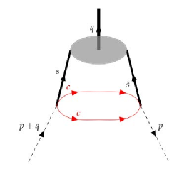
Figure 1: The leading order diagram contribute to $\Pi_{\mu}(p^{\prime},p,q)$.

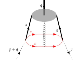
Figure 2: The one-gluon exchange contribution to $\Pi_{\mu}(p^{\prime},p,q)$.

FIG.1 represents the Feynman diagram of $\Pi_{\mu}(p^{\prime},p,q)$, represents the leading order contribution, which is dominant over the one-gluon exchange contribution in FIG.2, for instance. Therefore in Eq.(57), we only keep the leading order contribution.

Now, it is straightforward that one can evaluate the strong coupling by Using Eq.(52), and hence the decay width of $X(4500)$ $\to J/\psi\phi$ can be calculated through Eq.Dias:2013xfa

$$\Gamma^{\text{LC}}(X(4500)\to J/\psi\phi)=\frac{(\tilde{g}_{XJ/\psi\phi}^{LC})^{2}}{24\pi m_{X}^{2}}$$ (58)

$$\times\lambda(m_{X},m_{J/\psi},m_{\phi})\left(3+\frac{\lambda(m_{X},m_{J/\psi},m_{\phi})}{m^{2}_{J/\psi}}\right).$$

III Numerical calculation

III.1 Input parameters

After theoretical preparation, we commence the numerical calculations for the mass and the decay constant of $X(4500)$, and for the decay width of $X(4500)\to J/\psi\phi$ as well.

First, the values of the non-perturbative vacuum condensates are presented as Wang:2016gxp

$$\langle{\bar{q}q}\rangle=-(0.24\pm 0.01)^{3}\ \text{GeV}^{3},$$ (59)

$$\braket{\bar{s}s}=(0.8\pm 0.1)\times\braket{\bar{q}q},$$

$$\braket{g_{s}\bar{s}\sigma Gs}=m_{0}^{2}\times\braket{\bar{s}s},$$

$$m_{0}^{2}=0.8\ \text{GeV}^{2},$$

$$\braket{\frac{\alpha_{s}}{\pi}GG}=(0.012)\ \text{GeV}^{4}{\color[rgb]{1,0,0}.}$$

Second, we adopt the decay constants of $\phi$ and $J/\psi$ as $f_{\phi}^{\|}=0.215$ GeV Ball:2007zt and $f_{J/\psi}=0.405$ GeV Dias:2013xfa respectively. Meanwhile, from Particla Data Group (PDG) ParticleDataGroup:2020ssz , the current-quark-mass for the s-quark and charm-quark are taken as $m_{s}=93^{+11}_{-5}$ MeV and $m_{c}=(1.275\pm 0.025)$ GeV respectively, and, likewise, we accept the $J/\psi$-meson mass $m_{J/\psi}=(3096.900\pm 0.006)$ MeV and the $\phi$ mass $m_{\phi}=(990\pm 20)$ MeV. The parameters $\zeta_{4}^{\bot}$ and $\widetilde{\zeta}_{4}^{\bot}$ are taken as $\zeta_{4}^{\bot}=-0.01$ and $\widetilde{\zeta}_{4}^{\bot}=-0.03$ Ball:2007zt . Besides, for the Gegenbauer moments, we take $a_{1}^{\|}=a_{1}^{\bot}=0$, $a_{2}^{\|}=0.18$ and $a_{2}^{\bot}=0.14$ Ball:2007zt .

III.2 The mass and the decay constant

Since we consider $X$(4500) as a D-wave tetraquark state, the primary thing we need to know is whether our conjecture is tenable or not. So, before we evaluate the coupling, we should first evaluate the mass of $X(4500)$. In addition, we also need to figure out the decay constant of $X(4500)$ because it is an indispensable parameter for coupling.

There are two parameters that the sum rules predictions will depend on: the Borel mass $M^{2}$ and the continuum threshold $s_{0}$.

As a first step, $s_{0}$ can be determined by two principles:

1. The mass value of the considered hadron should rely on $s_{0}$ as weak as possible.

2. The $s_{0}$ should be related to the first excited states of hadron.

Because of the absence of experimental data of $X(4500)$, we cannot use the second principle directly. Although, one may naturaly chose $s_{0}=(m_{X}+0.5)^{2}$ $\rm GeV^{2}$, because the mass gap between the ground state and the first excited state is regularly around $0.5$ GeV in charmonia and bottomonia Olpak:2016wkf ; ParticleDataGroup:2012pjm , it may, however, not be true for $X(4500)$. So, the first principle become our primary choice.

We therefore define the function of

$$\Delta(M^{2},s_{0})=\left(\frac{\partial m_{X}}{\partial(M^{2})}\right)^{2}+\left(\frac{\partial m_{X}}{\partial(s_{0})}\right)^{2}$$ (60)

to describe the variation degree of the mass. In addition, we also impose the following constrain on $s_{0}$:

$$s_{0}<(m_{X}+1)^{2}\ \text{GeV}^{2},$$ (61)

since the energy gap between the ground state and the first excited state is usually smaller than 1 GeV Wu:2021tzo . Through the numerical calculation of $\Delta(M^{2},s_{0})$ with a varying range of $M^{2}$ and $s_{0}$, we found that, in a large range of $M^{2}$, the value of $\Delta(M^{2},s_{0})$ is close enough to the minimal value when $s_{0}$ is around $(m_{X}+0.398)^{2}\ \text{GeV}^{2}$. Therefore, for $X(4500)$, we employ

$$(4.90-0.10)^{2}\ \text{GeV}^{2}\leq s_{0}\leq(4.90+0.10)^{2}\ \text{GeV}^{2}.$$ (62)

Secondly, to determine the Borel mass $M^{2}$, we implement two criteria:

1. The contribution proportional to $\braket{\bar{q}g_{s}Gq}$ and higher dimension condensates should be less than $10\%$ of the gross contribution:

   $$\mathrm{CVG}\equiv\left|\frac{\tilde{\Pi}^{\braket{\bar{q}g_{s}Gq}+\cdots}\left(M^{2},\infty\right)}{\tilde{\Pi}^{OPE}\left(M^{2},\infty\right)}\right|\leq 10\%,$$ (63)

   where the dots means the terms with dimensions higher than $\braket{\bar{q}g_{s}Gq}$.

2. The pole contribution (PC) should exceed $70\%$:

   $$\text{PC}=\frac{\Pi^{SVZ,OPE}(M^{2},s_{0})}{\Pi^{SVZ,OPE}(M^{2},\infty)}\geq 70\%.$$ (64)

Those two criteria settle the minimal and maximal values of $M^{2}$ respectively.

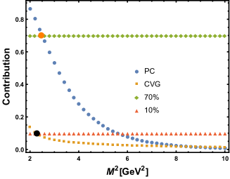
Figure 3: Convergence (CVG) and pole contribution (PC) for $X(4500)$.

The above criteria are shown in FIG.3. CVG and PC are represented in the yellow and blue curve respectively, they are both declining with the increase of $M^{2}$. The black dot indicates that the CVG intersects horizontally with the $10\%$ line, from which we can choose the minimum value of the Borel mass. Similarly, the orange dot indicates that the CVG reaches $70\%$, and we can determine the maximum value of the Borel mass. Therefore, the working region of the Borel mass turns to be

$$2.28\ \text{GeV}^{2}\leq M^{2}\leq 2.46\ \text{GeV}^{2}.$$ (65)

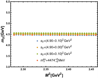
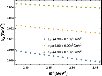
Figure 4: The mass [first] and the decay constant [second] of $X(4500)$ as a function of the Borel Mass $M^{2}$ at different fixed values of the continuum threshold $s_{0}$.

The calculation results of the mass and the decay constant have been depicted in Fig.4. We illustrate the results at fixed values of $s_{0}$$\in$$\{(4.90-0.10)^{2}\ \text{GeV}^{2}$, $(4.90+0.0)^{2}\ \text{GeV}^{2}$, $(4.90+0.1)^{2}\ \text{GeV}^{2}\}$ and show them with the blue, orange and green curves respectively. Base on the LHCb measurements LHCb:2021uow , $X(4500)$ has mass of $4474\pm 3\pm 3$ MeV. As shown in the figure, the blue, orange and green curves overlap with the experimental value in the working region of the Borel mass. At the central point of $M^{2}=2.37$ $\rm GeV^{2}$ and $s_{0}=(4.9+0.0)^{2}$ $\rm GeV^{2}$, the mass of $X(4500)$ can be extracted to be

$$\quad m_{X}=4.51^{+0.05}_{-0.04}\ \text{GeV}.$$ (66)

The uncertainty comes from the various condensates and the strange and charm quark masses. Our calculated results is consistent with the measurements of $X(4500)$. So it’s tenable that $X(4500)$ might be a D-wave $cs\bar{c}\bar{s}$ tetraquark.

Meanwhile, at the same benchmark point, our prediction of the decay constant is

$$\lambda_{X}\equiv m_{X}f_{X}=0.0521^{+0.0034}_{-0.0023}\ \text{GeV}^{7}.$$ (67)

Our next step is to calculate the decay width of $X$(4500)$\to J/\psi\phi$ using the mass and decay constant given above.

III.3 The coupling constant and the decay width

To determine the coupling constant $g_{XD_{s}^{*}D_{s}^{*}}$ we can fit the results with the analytical expression in the left-hand side with right-hand side of Eq[.(II.2)] and find $A=-0.0063\ \text{GeV}^{5},B=-5.3558\ \text{GeV}^{5},\ C=-0.3850\text{GeV}^{5},D=-3.6439\ \text{GeV}^{5}$ $E=0.0044\ \text{GeV}^{5}$, $F=0.4475\ \text{GeV}^{5}$. Using the definition in Eq.(II.2), we can obtain the values of coupling constants

$$g_{XD_{s}D_{s}} = -1.34884_{-0.083}^{+0.089}\ \text{GeV},$$

$$g_{XD_{s}^{*}D_{s}^{*}} = -1.44925^{+0.14}_{-0.15}\ \text{GeV},$$ (68)

$$g_{XD_{s}D_{s}^{*}} = 1.00197_{-0.165}^{+0.183}\ \text{GeV},$$

Therefor we obtain from Eq.(31):

$$\Gamma^{\text{LC}}(X(4500)\rightarrow D_{s}D_{s})=4.28^{+0.54}_{-0.51}\ \text{MeV}$$

$$\Gamma^{\text{LC}}(X(4500)\rightarrow D_{s}^{*}D_{s}^{*})=3.32^{+0.61}_{-0.73}\ \text{MeV}$$ (70)

$$\Gamma^{\text{LC}}(X(4500)\rightarrow D_{s}D_{s}^{*})=2.02^{+0.26}_{-0.71}\ \text{MeV}$$ (71)

In order to obtain the coupling constant of $\hat{g}_{XJ/\psi\phi}^{TP}$ from the three-point sum rules, we need to determine the continuum threshold $s_{0}$, the Borel mass $M^{2}$ and $Q^{2}=-q^{2}$ where $q^{2}$ represents the momentum of $\phi$. The same value of $s_{0}$ can be used as we have obtained in the two-point sum rules, so that Eq.(62) is applied.

As we see in Eq.(II.3), the coupling constant $\hat{g}_{XJ/\psi\phi}^{TP}$ depends on two parameters, $Q^{2}$ and $M^{2}$. An ideal working region can be determined by the fact that $\hat{g}_{XJ/\psi\phi}^{TP}$ should be independent as much as possible of $M^{2}$. In FIG.5, we show the $\hat{g}_{XJ/\psi\phi}^{TP}$ as functions of $M^{2}$ in the contour map. As shown in the picture, the contour lines have Extreme Values of $M^{2}$ while

$$3\ \text{GeV}^{2}\leq M^{2}\leq 5\ \text{GeV}^{2}$$ (73)

and

$$Q^{2}\geq 8\ \text{GeV}^{2}.$$ (74)

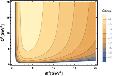
Figure 5: The strong coupling $\hat{g}_{XJ/\psi\phi}^{TP}$ of a $X(4500)$ as a function of the $M^{2}$ and $Q^{2}$.

Since the coupling constant is defined as the form factor at the pole of $Q^{2}=-m_{\phi}^{2}$, $\hat{g}_{XJ/\psi\phi}^{TP}$ should be extracted from $Q^{2}=-m_{\phi}^{2}$ where the sum rules results become infinity and invalid. However, our goal can be achieved by parametrizing the $\hat{g}_{XJ/\psi\phi}^{TP}$ with the help of Dias:2013xfa :

$$\hat{g}_{XJ/\psi\phi}^{TP}=A_{1}e^{-\frac{A_{2}}{Q^{2}}}.$$ (75)

What we have to do is fitting the results of $\hat{g}_{XJ/\psi\phi}^{TP}$ in the region of $Q^{2}\geq 8\ \text{GeV}^{2}$ with the above equation. Here, for convenient, we choose the region to be $8\ \text{GeV}^{2}\leq Q^{2}\leq 10\ \text{GeV}^{2}$. After those preparations, we can solve out $A_{1}$ and $A_{2}$ and receive the vaules that $A_{1}=7.9638$ and $A_{2}=90.698$. And we calculate the value $\hat{g}_{XJ/\psi\phi}^{TP}$ from $Q^{2}=-m_{\phi}^{2}$. The exponential form of $\hat{g}_{XJ/\psi\phi}^{TP}$ is pictured in Fig.6. Fig.6 shows the $Q^{2}$ dependence of $\hat{g}_{XJ/\psi\phi}^{TP}$ while we set $M^{2}=6.0$ $\rm GeV^{2}$. For other values of $M^{2}$, the results are similar in the range of $5$ $\rm GeV^{2}$ $\leq M^{2}\leq 9$ $\rm GeV^{2}$. The purple dots are the data we tried to fit and the red one shows the results at $Q^{2}=-m_{\phi}^{2}$:

$$\hat{g}_{XJ/\psi\phi}^{TP}=-8.047^{+0.41}_{-0.42}\mathrm{GeV}.$$ (76)

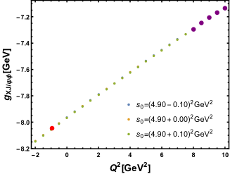
Figure 6: The exponential form of $\hat{g}_{XJ/\psi\phi}^{TP}$ as a function of the Borel Mass $Q^{2}$ at different fixed values of $s_{0}$ while $M^{2}=4.0$ GeV².

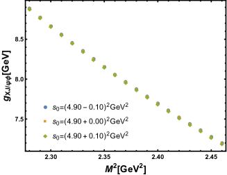
Figure 7: The strong coupling $\tilde{g}_{XJ/\psi\phi}^{LC}$ in light-cone sum rules as a function of the Borel Mass $M^{2}$ at different fixed values of $s_{0}$.

Next, we pay attention to the coupling constant of $g_{XJ/\psi\phi}$ in the light-cone sum rules. For $M^{2}$ and $s_{0}$, we use the same values as in the analysis of the mass. The prediction for $\tilde{g}_{XJ/\psi\phi}^{LC}$ is

$$\tilde{g}_{XJ/\psi\phi}^{LC}=7.796^{+1.191}_{-0.583}\ \text{GeV}.$$ (77)

By using the Eq.(52), the width of $X$(4500) $\to$ $J/\psi\phi$ are obtained to be

$$\Gamma^{\text{TP}}(X(4500)\rightarrow J/\psi\phi)=124.32^{+12}_{-13}\ \text{MeV}$$ (78)

and

$$\Gamma^{\text{LC}}(X(4500)\rightarrow J/\psi\phi)=116_{-38}^{+17}\ \text{MeV}$$ (79)

for the three-point sum rules and the light-cone sum rules respectively. Base on the experiment LHCb:2021uow , $X(4500)$ has total width of $77\pm 6^{+10}_{-8}$ $\rm MeV$. Both of the three-point sum rules prediction and that of the LCSR are close with the total width of $X$(4500) within the error. From the calculation of $X(4500)\to D_{s}D_{s}$, $X(4500)\to D_{s}^{*}D_{s}$, and $X(4500)\to D_{s}^{*}D_{s}^{*}$, we can see the widths are much smaller than that of $X$(4500) $\to$ $J/\psi\phi$. The results of the open-charm decay channels, combined with the results of the hidden-charm decay channel, do not exceed the total width of the state. This suggest that the hidden-charm decay channels $X(4500)$ $\to$ $J/\psi\phi$ are predominant when compared with the total width of $X(4500)$ when we assign $X(4500)$ as a D-wave $cs\bar{c}\bar{s}$ tetraquark state. Moreover, calculating the complete open-charm decay will provide a more rational conclusion. If all those widths of open and hidden decays are consistent with the total width of $X(4500)$, the D-wave assignment for $X(4500)$ may be appropriate, and $X$(4500) $\to$ $J/\psi\phi$ will be its most significant decay channel. Fulture experiments are needed to further determine the structure of $X(4500)$.

IV Summary

By assigning a D-wave tetraquark state to $X$(4500), we investigate its mass, decay constant, and its decay of $X(4500)\to J/\psi\phi$ in this paper. By evaluating the mass of $X(4500)$ via the two-point sum rules, we found that the result was consistent with that in PDG. Meanwhile, the decay constant of $X(4500)$ has also been calculated. Then through both the approaches of the light-cone sum rules and the three-point sum rules, we calculate the strong coupling constant of $g_{XJ/\psi\phi}$ and obtain the decay width. In the case of D-wave tetraquarks, $X(4500)\to J/\psi\phi$ will be close to the total width of $X(4500)$. Since our approach focuses exclusively on hidden-charm meson decay in this paper, so we recommends calculating open-charm decays when $X(4500)$ is assigned as a state of D-wave tetraquarks. D-wave interpretation is not appropriate for state $X(4500)$ when results from the open-charm decay channels plus those from the hidden decay channel exceed the width of the state. Else we can conclude that D-wave tetraquark state may be appropriate for $X(4500)$ and that $X(4500)\to J/\psi\phi$ is the predominant process. The results are instructive for future experiments to further determine the structure of $X(4500)$.

V Appendix

V.1 OPE results of open-charm decays

$$\Pi^{DD}_{1}(M^{2})=$$ (80)

$$-\frac{8\pi^{8}m_{c}^{2}m_{s}^{2}\langle\bar{q}g_{s}\sigma Gq\rangle\langle\bar{q}q\rangle e^{-\frac{m_{c}^{2}}{M^{2}}}}{M^{4}}+\frac{128\pi^{9}\alpha_{s}m_{c}^{2}m_{s}\langle\bar{q}q\rangle^{3}e^{-\frac{m_{c}^{2}}{M^{2}}}}{27M^{4}}$$

$$+\frac{\pi^{8}m_{c}^{6}m_{s}^{2}\langle\bar{q}g_{s}\sigma Gq\rangle^{2}e^{-\frac{m_{c}^{2}}{M^{2}}}}{15M^{10}}-\frac{16\pi^{9}\alpha_{s}m_{c}^{6}m_{s}\langle\bar{q}g_{s}\sigma Gq\rangle\langle\bar{q}q\rangle^{2}e^{-\frac{m_{c}^{2}}{M^{2}}}}{405M^{10}}$$

$$-\frac{\pi^{8}m_{c}^{4}m_{s}^{2}\langle\bar{q}g_{s}\sigma Gq\rangle^{2}e^{-\frac{m_{c}^{2}}{M^{2}}}}{3M^{8}}+\frac{16\pi^{9}\alpha_{s}m_{c}^{4}m_{s}\langle\bar{q}g_{s}\sigma Gq\rangle\langle\bar{q}q\rangle^{2}e^{-\frac{m_{c}^{2}}{M^{2}}}}{81M^{8}}$$

$$+\frac{8\pi^{8}m_{c}^{4}m_{s}^{2}\langle\bar{q}g_{s}\sigma Gq\rangle\langle\bar{q}q\rangle e^{-\frac{m_{c}^{2}}{M^{2}}}}{3M^{6}}-\frac{128\pi^{9}\alpha_{s}m_{c}^{4}m_{s}\langle\bar{q}q\rangle^{3}e^{-\frac{m_{c}^{2}}{M^{2}}}}{81M^{6}}$$

$$\Pi^{DD}_{2}(M^{2})=\int_{4m_{c}^{2}}^{s_{0}}e^{-s/M^{2}}ds$$ (81)

$$\frac{32m_{s}\pi^{8}\langle\bar{q}g_{s}\sigma Gq\rangle\langle\bar{q}q\rangle sm_{c}^{9}}{\left(m^{2}-s\right)^{7}}-\frac{512\pi^{9}\langle\bar{q}q\rangle^{3}s\alpha_{s}m_{c}^{9}}{27\left(m_{c}^{2}-s\right)^{7}}$$

$$+\frac{320\langle g_{s}^{2}GG\rangle\pi^{10}\langle\bar{q}q\rangle^{2}sm_{c}^{8}}{3\left(m^{2}-s\right)^{7}}+\frac{12m_{s}\pi^{8}\langle\bar{q}g_{s}\sigma Gq\rangle^{2}sm_{c}^{7}}{\left(m_{c}^{2}-s\right)^{7}}$$

$$+\frac{32\langle g_{s}^{2}GG\rangle m_{s}\pi^{10}\langle\bar{q}q\rangle^{2}sm_{c}^{7}}{3\left(m_{c}^{2}-s\right)^{7}}+\frac{2048\pi^{9}\langle\bar{q}q\rangle^{3}s^{2}\alpha_{s}m_{c}^{7}}{27\left(m_{c}^{2}-s\right)^{7}}$$

$$-\frac{128m_{s}\pi^{8}\langle\bar{q}g_{s}\sigma Gq\rangle\langle\bar{q}q\rangle s^{2}m_{c}^{7}}{\left(m_{c}^{2}-s\right)^{7}}-\frac{64\pi^{9}\langle\bar{q}g_{s}\sigma Gq\rangle\langle\bar{q}q\rangle^{2}s\alpha_{s}m_{c}^{7}}{9\left(m_{c}^{2}-s\right)^{7}}$$

$$+\frac{40\langle g_{s}^{2}GG\rangle\pi^{10}\langle\bar{q}g_{s}\sigma Gq\rangle\langle\bar{q}q\rangle sm_{c}^{6}}{\left(m_{c}^{2}-s\right)^{7}}$$

$$-\frac{3200\langle g_{s}^{2}GG\rangle\pi^{10}\langle\bar{q}q\rangle^{2}s^{2}m_{c}^{6}}{9\left(m_{c}^{2}-s\right)^{7}}$$

$$+\frac{192m_{s}\pi^{8}\langle\bar{q}g_{s}\sigma Gq\rangle\langle\bar{q}q\rangle s^{3}m_{c}^{5}}{\left(m_{c}^{2}-s\right)^{7}}$$

$$+\frac{16\langle g_{s}^{2}GG\rangle m_{s}\pi^{10}\langle\bar{q}g_{s}\sigma Gq\rangle\langle\bar{q}q\rangle sm_{c}^{5}}{3\left(m_{c}^{2}-s\right)^{7}}$$

$$+\frac{448\pi^{9}\langle\bar{q}g_{s}\sigma Gq\rangle\langle\bar{q}q\rangle^{2}s^{2}\alpha_{s}m_{c}^{5}}{27\left(m_{c}^{2}-s\right)^{7}}-\frac{28m_{s}\pi^{8}\langle\bar{q}g_{s}\sigma Gq\rangle^{2}s^{2}m_{c}^{5}}{\left(m_{c}^{2}-s\right)^{7}}$$

$$-\frac{224\langle g_{s}^{2}GG\rangle m_{s}\pi^{10}\langle\bar{q}q\rangle^{2}s^{2}m_{c}^{5}}{9\left(m_{c}^{2}-s\right)^{7}}-\frac{1024\pi^{9}\langle\bar{q}q\rangle^{3}s^{3}\alpha_{s}m_{c}^{5}}{9\left(m_{c}^{2}-s\right)^{7}}$$

$$+\frac{1280\langle g_{s}^{2}GG\rangle\pi^{10}\langle\bar{q}q\rangle^{2}s^{3}m_{c}^{4}}{3\left(m_{c}^{2}-s\right)^{7}}$$

$$-\frac{200\langle g_{s}^{2}GG\rangle\pi^{10}\langle\bar{q}g_{s}\sigma Gq\rangle\langle\bar{q}q\rangle s^{2}m_{c}^{4}}{3\left(m_{c}^{2}-s\right)^{7}}$$

$$+\frac{20m_{s}\pi^{8}\langle\bar{q}g_{s}\sigma Gq\rangle^{2}s^{3}m_{c}^{3}}{\left(m_{c}^{2}-s\right)^{7}}+\frac{160\langle g_{s}^{2}GG\rangle m_{s}\pi^{10}\langle\bar{q}q\rangle^{2}s^{3}m_{c}^{3}}{9\left(m_{c}^{2}-s\right)^{7}}$$

$$+\frac{2048\pi^{9}\langle\bar{q}q\rangle^{3}s^{4}\alpha_{s}m_{c}^{3}}{27\left(m_{c}^{2}-s\right)^{7}}-\frac{128m_{s}\pi^{8}\langle\bar{q}g_{s}\sigma Gq\rangle\langle\bar{q}q\rangle s^{4}m_{c}^{3}}{\left(m_{c}^{2}-s\right)^{7}}$$

$$-\frac{16\langle g_{s}^{2}GG\rangle m_{s}\pi^{10}\langle\bar{q}g_{s}\sigma Gq\rangle\langle\bar{q}q\rangle s^{2}m_{c}^{3}}{9\left(m_{c}^{2}-s\right)^{7}}$$

$$-\frac{320\pi^{9}\langle\bar{q}g_{s}\sigma Gq\rangle\langle\bar{q}q\rangle^{2}s^{3}\alpha_{s}m_{c}^{3}}{27\left(m_{c}^{2}-s\right)^{7}}$$

$$+\frac{280\langle g_{s}^{2}GG\rangle\pi^{10}\langle\bar{q}g_{s}\sigma Gq\rangle\langle\bar{q}q\rangle s^{3}m_{c}^{2}}{9\left(m_{c}^{2}-s\right)^{7}}$$

$$-\frac{640\langle g_{s}^{2}GG\rangle\pi^{10}\langle\bar{q}q\rangle^{2}s^{4}m_{c}^{2}}{3\left(m_{c}^{2}-s\right)^{7}}$$

$$+\frac{32m_{s}\pi^{8}\langle\bar{q}g_{s}\sigma Gq\rangle\langle\bar{q}q\rangle s^{5}m_{c}}{\left(m_{c}^{2}-s\right)^{7}}+\frac{64\pi^{9}\langle\bar{q}g_{s}\sigma Gq\rangle\langle\bar{q}q\rangle^{2}s^{4}\alpha_{s}m_{c}}{27\left(m_{c}^{2}-s\right)^{7}}$$

$$-\frac{4m_{s}\pi^{8}\langle\bar{q}g_{s}\sigma Gq\rangle^{2}s^{4}m_{c}}{\left(m_{c}^{2}-s\right)^{7}}-\frac{32\langle g_{s}^{2}GG\rangle m_{s}\pi^{10}\langle\bar{q}q\rangle^{2}s^{4}m_{c}}{9\left(m_{c}^{2}-s\right)^{7}}$$

$$-\frac{512\pi^{9}\langle\bar{q}q\rangle^{3}s^{5}\alpha_{s}m_{c}}{27\left(m_{c}^{2}-s\right)^{7}}+\frac{320\langle g_{s}^{2}GG\rangle\pi^{10}\langle\bar{q}q\rangle^{2}s^{5}}{9\left(m_{c}^{2}-s\right)^{7}}$$

$$-\frac{40\langle g_{s}^{2}GG\rangle\pi^{10}\langle\bar{q}g_{s}\sigma Gq\rangle\langle\bar{q}q\rangle s^{4}}{9\left(m_{c}^{2}-s\right)^{7}}$$

$$\Pi^{DDs}_{1}(M^{2})=$$ (82)

$$\frac{20\pi^{10}\langle g_{s}^{2}GG\rangle m_{c}^{2}\langle\bar{q}g_{s}\sigma Gq\rangle\langle\bar{q}q\rangle e^{-\frac{m_{c}^{2}}{M^{2}}}}{9M^{6}}$$

$$+\frac{16\pi^{10}\langle g_{s}^{2}GG\rangle m_{c}m_{s}\langle\bar{q}q\rangle^{2}e^{-\frac{m_{c}^{2}}{M^{2}}}}{9M^{4}}$$

$$+\frac{20\pi^{10}\langle g_{s}^{2}GG\rangle\langle\bar{q}g_{s}\sigma Gq\rangle\langle\bar{q}q\rangle e^{-\frac{m_{c}^{2}}{M^{2}}}}{9M^{4}}$$

$$+\frac{160\pi^{10}\langle g_{s}^{2}GG\rangle m_{c}^{2}\langle\bar{q}q\rangle^{2}e^{-\frac{m_{c}^{2}}{M^{2}}}}{9M^{4}}$$

$$+\frac{320\pi^{10}\langle g_{s}^{2}GG\rangle\langle\bar{q}q\rangle^{2}e^{-\frac{m_{c}^{2}}{M^{2}}}}{9M^{2}}$$

$$-\frac{2\pi^{10}\langle g_{s}^{2}GG\rangle m_{c}^{7}m_{s}\langle\bar{q}g_{s}\sigma Gq\rangle\langle\bar{q}q\rangle e^{-\frac{m_{c}^{2}}{M^{2}}}}{405M^{1}2}$$

$$-\frac{4\pi^{10}\langle g_{s}^{2}GG\rangle m_{c}^{6}\langle\bar{q}g_{s}\sigma Gq\rangle\langle\bar{q}q\rangle e^{-\frac{m_{c}^{2}}{M^{2}}}}{27M^{1}0}$$

$$+\frac{2\pi^{10}\langle g_{s}^{2}GG\rangle m_{c}^{5}m_{s}\langle\bar{q}g_{s}\sigma Gq\rangle\langle\bar{q}q\rangle e^{-\frac{m_{c}^{2}}{M^{2}}}}{135M^{1}0}$$

$$-\frac{8\pi^{10}\langle g_{s}^{2}GG\rangle m_{c}^{5}m_{s}\langle\bar{q}q\rangle^{2}e^{-\frac{m_{c}^{2}}{M^{2}}}}{27M^{8}}$$

$$-\frac{320\pi^{10}\langle g_{s}^{2}GG\rangle m_{c}^{4}\langle\bar{q}q\rangle^{2}e^{-\frac{m_{c}^{2}}{M^{2}}}}{27M^{6}}$$

$$+\frac{2\pi^{10}\langle g_{s}^{2}GG\rangle m_{c}^{3}m_{s}\langle\bar{q}g_{s}\sigma Gq\rangle\langle\bar{q}q\rangle e^{-\frac{m_{c}^{2}}{M^{2}}}}{27M^{8}}$$

$$+\frac{16\pi^{10}\langle g_{s}^{2}GG\rangle m_{c}^{3}m_{s}\langle\bar{q}q\rangle^{2}e^{-\frac{m_{c}^{2}}{M^{2}}}}{27M^{6}}$$

$$+\frac{2\pi^{8}m_{c}m_{s}\langle\bar{q}g_{s}\sigma Gq\rangle^{2}e^{-\frac{m_{c}^{2}}{M^{2}}}}{M^{4}}-\frac{32\pi^{9}\alpha_{s}m_{c}\langle\bar{q}g_{s}\sigma Gq\rangle\langle\bar{q}q\rangle^{2}e^{-\frac{m_{c}^{2}}{M^{2}}}}{27M^{4}}+$$

$$\frac{32\pi^{8}m_{c}m_{s}\langle\bar{q}g_{s}\sigma Gq\rangle\langle\bar{q}q\rangle e^{-\frac{m_{c}^{2}}{M^{2}}}}{M^{2}}-\frac{512\pi^{9}\alpha_{s}m_{c}\langle\bar{q}q\rangle^{3}e^{-\frac{m_{c}^{2}}{M^{2}}}}{27M^{2}}$$

$$-\frac{\pi^{8}m_{c}^{5}m_{s}\langle\bar{q}g_{s}\sigma Gq\rangle^{2}e^{-\frac{m_{c}^{2}}{M^{2}}}}{3M^{8}}+\frac{16\pi^{9}\alpha_{s}m_{c}^{5}\langle\bar{q}g_{s}\sigma Gq\rangle\langle\bar{q}q\rangle^{2}e^{-\frac{m_{c}^{2}}{M^{2}}}}{81M^{8}}$$

$$+\frac{2\pi^{8}m_{c}^{3}m_{s}\langle\bar{q}g_{s}\sigma Gq\rangle^{2}e^{-\frac{m_{c}^{2}}{M^{2}}}}{3M^{6}}-\frac{32\pi^{9}\alpha_{s}m_{c}^{3}\langle\bar{q}g_{s}\sigma Gq\rangle\langle\bar{q}q\rangle^{2}e^{-\frac{m_{c}^{2}}{M^{2}}}}{81M^{6}}$$

$$-\frac{16\pi^{8}m_{c}^{3}m_{s}\langle\bar{q}g_{s}\sigma Gq\rangle\langle\bar{q}q\rangle e^{-\frac{m_{c}^{2}}{M^{2}}}}{M^{4}}+\frac{256\pi^{9}\alpha_{s}m_{c}^{3}\langle\bar{q}q\rangle^{3}e^{-\frac{m_{c}^{2}}{M^{2}}}}{27M^{4}}$$

$$\Pi^{DDs}_{2}(M^{2})=0$$ (83)

$$\Pi^{DsDs}_{1}(M^{2})=$$ (84)

$$\frac{64\pi^{10}\langle g_{s}^{2}GG\rangle m_{c}^{2}\langle\bar{q}q\rangle^{2}e^{-\frac{m_{c}^{2}}{M^{2}}}}{27M^{4}}$$

$$-\frac{8\pi^{10}\langle g_{s}^{2}GG\rangle m_{c}^{8}\langle\bar{q}g_{s}\sigma Gq\rangle\langle\bar{q}q\rangle e^{-\frac{m_{c}^{2}}{M^{2}}}}{2835M^{14}}$$

$$\frac{64\pi^{10}\langle g_{s}^{2}GG\rangle m_{c}^{2}\langle\bar{q}q\rangle^{2}e^{-\frac{m_{c}^{2}}{M^{2}}}}{27M^{4}}$$

$$-\frac{8\pi^{10}\langle g_{s}^{2}GG\rangle m_{c}^{8}\langle\bar{q}g_{s}\sigma Gq\rangle\langle\bar{q}q\rangle e^{-\frac{m_{c}^{2}}{M^{2}}}}{2835M^{14}}$$

$$+\frac{4\pi^{10}\langle g_{s}^{2}GG\rangle m_{c}^{6}\langle\bar{q}g_{s}\sigma Gq\rangle\langle\bar{q}q\rangle e^{-\frac{m_{c}^{2}}{M^{2}}}}{81M^{12}}$$

$$-\frac{2\pi^{10}\langle g_{s}^{2}GG\rangle m_{c}^{6}\langle\bar{q}g_{s}\sigma Gq\rangle\langle\bar{q}q\rangle e^{-\frac{m_{c}^{2}}{M^{2}}}}{405M^{10}}$$

$$-\frac{16\pi^{10}\langle g_{s}^{2}GG\rangle m_{c}^{4}\langle\bar{q}g_{s}\sigma Gq\rangle\langle\bar{q}q\rangle e^{-\frac{m_{c}^{2}}{M^{2}}}}{135M^{10}}$$

$$+\frac{4\pi^{10}\langle g_{s}^{2}GG\rangle m_{c}^{4}\langle\bar{q}g_{s}\sigma Gq\rangle\langle\bar{q}q\rangle e^{-\frac{m_{c}^{2}}{M^{2}}}}{81M^{8}}$$

$$-\frac{32\pi^{10}\langle g_{s}^{2}GG\rangle m_{c}^{4}\langle\bar{q}q\rangle^{2}e^{-\frac{m_{c}^{2}}{M^{2}}}}{81M^{6}}$$

$$-\frac{16\pi^{8}m_{c}^{2}m_{s}^{2}\langle\bar{q}g_{s}\sigma Gq\rangle\langle\bar{q}q\rangle e^{-\frac{m^{2}}{M^{2}}}}{3M^{4}}$$

$$+\frac{256\pi^{9}\alpha_{s}m_{c}^{2}m_{s}\langle\bar{q}q\rangle^{3}e^{-\frac{m_{c}^{2}}{M^{2}}}}{81M^{4}}$$

$$+\frac{8\pi^{8}m_{c}^{8}m_{s}^{2}\langle\bar{q}g_{s}\sigma Gq\rangle^{2}e^{-\frac{m_{c}^{2}}{M^{2}}}}{189M^{14}}$$

$$-\frac{128\pi^{9}\alpha_{s}m_{c}^{8}m_{s}\langle\bar{q}g_{s}\sigma Gq\rangle\langle\bar{q}q\rangle^{2}e^{-\frac{m_{c}^{2}}{M^{2}}}}{5103M^{14}}$$

$$-\frac{56\pi^{8}m_{c}^{6}m_{s}^{2}\langle\bar{q}g_{s}\sigma Gq\rangle^{2}e^{-\frac{m_{c}^{2}}{M^{2}}}}{135M^{12}}$$

$$+\frac{896\pi^{9}\alpha_{s}m_{c}^{6}m_{s}\langle\bar{q}g_{s}\sigma Gq\rangle\langle\bar{q}q\rangle^{2}e^{-\frac{m_{c}^{2}}{M^{2}}}}{3645M^{1}2}$$

$$+\frac{2\pi^{8}m_{c}^{6}m_{s}^{2}\langle\bar{q}g_{s}\sigma Gq\rangle^{2}e^{-\frac{m_{c}^{2}}{M^{2}}}}{45M^{10}}$$

$$-\frac{32\pi^{9}\alpha_{s}m_{c}^{6}m_{s}\langle\bar{q}g_{s}\sigma Gq\rangle\langle\bar{q}q\rangle^{2}e^{-\frac{m_{c}^{2}}{M^{2}}}}{1215M^{10}}$$

$$+\frac{32\pi^{8}m_{c}^{4}m_{s}^{2}\langle\bar{q}g_{s}\sigma Gq\rangle^{2}e^{-\frac{m_{c}^{2}}{M^{2}}}}{45M^{10}}$$

$$-\frac{512\pi^{9}\alpha_{s}m_{c}^{4}m_{s}\langle\bar{q}g_{s}\sigma Gq\rangle\langle\bar{q}q\rangle^{2}e^{-\frac{m_{c}^{2}}{M^{2}}}}{1215M^{10}}$$

$$-\frac{2\pi^{8}m_{c}^{4}m_{s}^{2}\langle\bar{q}g_{s}\sigma Gq\rangle^{2}e^{-\frac{m_{c}^{2}}{M^{2}}}}{9M^{8}}$$

$$+\frac{32\pi^{9}\alpha_{s}m_{c}^{4}m_{s}\langle\bar{q}g_{s}\sigma Gq\rangle\langle\bar{q}q\rangle^{2}e^{-\frac{m_{c}^{2}}{M^{2}}}}{243M^{8}}$$

$$+\frac{16\pi^{8}m_{c}^{4}m_{s}^{2}\langle\bar{q}g_{s}\sigma Gq\rangle\langle\bar{q}q\rangle e^{-\frac{m_{c}^{2}}{M^{2}}}}{9M^{6}}$$

$$-\frac{256\pi^{9}\alpha_{s}m_{c}^{4}m_{s}\langle\bar{q}q\rangle^{3}e^{-\frac{m_{c}^{2}}{M^{2}}}}{243M^{6}}$$

$$\Pi^{DsDs}_{2}(M^{2})=\int_{4m_{c}^{2}}^{u_{0}}e^{-s/M^{2}}ds$$ (85)

$$\frac{64m_{s}\pi^{8}\langle\bar{q}g_{s}\sigma Gq\rangle\langle\bar{q}q\rangle m^{15}}{3\left(m^{2}-s\right)^{9}}-\frac{1024\pi^{9}\langle\bar{q}q\rangle^{3}\alpha_{s}m^{15}}{81\left(m^{2}-s\right)^{9}}$$

$$+\frac{256m_{s}\pi^{9}\langle\bar{q}q\rangle^{3}\alpha_{s}m^{14}}{81\left(m^{2}-s\right)^{9}}-\frac{16m_{s}^{2}\pi^{8}\langle\bar{q}g_{s}\sigma Gq\rangle\langle\bar{q}q\rangle m^{14}}{3\left(m^{2}-s\right)^{9}}$$

$$+\frac{5888\pi^{9}\langle\bar{q}q\rangle^{3}s\alpha_{s}m^{13}}{81\left(m^{2}-s\right)^{9}}+\frac{16m_{s}\pi^{8}\langle\bar{q}g_{s}\sigma Gq\rangle^{2}m^{13}}{3\left(m^{2}-s\right)^{9}}$$

$$-\frac{368m_{s}\pi^{8}\langle\bar{q}g_{s}\sigma Gq\rangle\langle\bar{q}q\rangle sm^{13}}{3\left(m^{2}-s\right)^{9}}-\frac{64\langle g_{s}^{2}GG\rangle m_{s}\pi^{10}\langle\bar{q}q\rangle^{2}m^{13}}{27\left(m^{2}-s\right)^{9}}$$

$$-\frac{256\pi^{9}\langle\bar{q}g_{s}\sigma Gq\rangle\langle\bar{q}q\rangle^{2}\alpha_{s}m^{13}}{81\left(m^{2}-s\right)^{9}}+\frac{32m_{s}^{2}\pi^{8}\langle\bar{q}g_{s}\sigma Gq\rangle\langle\bar{q}q\rangle sm^{12}}{\left(m^{2}-s\right)^{9}}$$

$$+\frac{448\langle g_{s}^{2}GG\rangle\pi^{10}\langle\bar{q}q\rangle^{2}sm^{12}}{9\left(m^{2}-s\right)^{9}}+\frac{1024m_{s}\pi^{9}\langle\bar{q}q\rangle^{3}\alpha_{s}m^{12}}{27\left(m^{2}-s\right)^{9}}$$

$$-\frac{64m_{s}^{2}\pi^{8}\langle\bar{q}g_{s}\sigma Gq\rangle\langle\bar{q}q\rangle m^{12}}{\left(m^{2}-s\right)^{9}}+\frac{4m_{s}^{2}\pi^{8}\langle\bar{q}g_{s}\sigma Gq\rangle^{2}m^{12}}{3\left(m^{2}-s\right)^{9}}$$

$$-\frac{512m_{s}\pi^{9}\langle\bar{q}q\rangle^{3}s\alpha_{s}m^{12}}{27\left(m^{2}-s\right)^{9}}-\frac{64m_{s}\pi^{9}\langle\bar{q}g_{s}\sigma Gq\rangle\langle\bar{q}q\rangle^{2}\alpha_{s}m^{12}}{81\left(m^{2}-s\right)^{9}}$$

$$+\frac{288m_{s}\pi^{8}\langle\bar{q}g_{s}\sigma Gq\rangle\langle\bar{q}q\rangle s^{2}m^{11}}{\left(m^{2}-s\right)^{9}}$$

$$+\frac{464\langle g_{s}^{2}GG\rangle m_{s}\pi^{10}\langle\bar{q}q\rangle^{2}sm^{11}}{27\left(m^{2}-s\right)^{9}}$$

$$+\frac{832\pi^{9}\langle\bar{q}g_{s}\sigma Gq\rangle\langle\bar{q}q\rangle^{2}s\alpha_{s}m^{11}}{81\left(m^{2}-s\right)^{9}}+\frac{64m_{s}\pi^{8}\langle\bar{q}g_{s}\sigma Gq\rangle^{2}m^{11}}{\left(m^{2}-s\right)^{9}}$$

$$-\frac{52m_{s}\pi^{8}\langle\bar{q}g_{s}\sigma Gq\rangle^{2}sm^{11}}{3\left(m^{2}-s\right)^{9}}-\frac{512\pi^{9}\langle\bar{q}q\rangle^{3}s^{2}\alpha_{s}m^{11}}{3\left(m^{2}-s\right)^{9}}$$

$$-\frac{64\langle g_{s}^{2}GG\rangle m_{s}\pi^{10}\langle\bar{q}q\rangle^{2}m^{11}}{9\left(m^{2}-s\right)^{9}}$$

$$-\frac{8\langle g_{s}^{2}GG\rangle m_{s}\pi^{10}\langle\bar{q}g_{s}\sigma Gq\rangle\langle\bar{q}q\rangle m^{11}}{27\left(m^{2}-s\right)^{9}}$$

$$-\frac{1024\pi^{9}\langle\bar{q}g_{s}\sigma Gq\rangle\langle\bar{q}q\rangle^{2}\alpha_{s}m^{11}}{27\left(m^{2}-s\right)^{9}}+\frac{240m_{s}^{2}\pi^{8}\langle\bar{q}g_{s}\sigma Gq\rangle\langle\bar{q}q\rangle sm^{10}}{\left(m^{2}-s\right)^{9}}$$

$$+\frac{56\langle g_{s}^{2}GG\rangle\pi^{10}\langle\bar{q}g_{s}\sigma Gq\rangle\langle\bar{q}q\rangle sm^{10}}{3\left(m^{2}-s\right)^{9}}+\frac{3904m_{s}\pi^{9}\langle\bar{q}q\rangle^{3}s^{2}\alpha_{s}m^{10}}{81\left(m^{2}-s\right)^{9}}$$

$$+\frac{928m_{s}\pi^{9}\langle\bar{q}g_{s}\sigma Gq\rangle\langle\bar{q}q\rangle^{2}s\alpha_{s}m^{10}}{243\left(m^{2}-s\right)^{9}}+\frac{64m_{s}^{2}\pi^{8}\langle\bar{q}g_{s}\sigma Gq\rangle^{2}m^{10}}{3\left(m^{2}-s\right)^{9}}$$

$$-\frac{244m_{s}^{2}\pi^{8}\langle\bar{q}g_{s}\sigma Gq\rangle\langle\bar{q}q\rangle s^{2}m^{10}}{3\left(m^{2}-s\right)^{9}}-\frac{58m_{s}^{2}\pi^{8}\langle\bar{q}g_{s}\sigma Gq\rangle^{2}sm^{10}}{9\left(m^{2}-s\right)^{9}}$$

$$-\frac{1280m_{s}\pi^{9}\langle\bar{q}q\rangle^{3}s\alpha_{s}m^{10}}{9\left(m^{2}-s\right)^{9}}-\frac{7168\langle g_{s}^{2}GG\rangle\pi^{10}\langle\bar{q}q\rangle^{2}s^{2}m^{10}}{27\left(m^{2}-s\right)^{9}}$$

$$-\frac{1024m_{s}\pi^{9}\langle\bar{q}g_{s}\sigma Gq\rangle\langle\bar{q}q\rangle^{2}\alpha_{s}m^{10}}{81\left(m^{2}-s\right)^{9}}+\frac{40m_{s}\pi^{8}\langle\bar{q}g_{s}\sigma Gq\rangle^{2}s^{2}m^{9}}{3\left(m^{2}-s\right)^{9}}$$

$$+\frac{16m_{s}\pi^{8}\langle\bar{q}g_{s}\sigma Gq\rangle^{2}sm^{9}}{\left(m^{2}-s\right)^{9}}+\frac{256\langle g_{s}^{2}GG\rangle m_{s}\pi^{10}\langle\bar{q}q\rangle^{2}sm^{9}}{9\left(m^{2}-s\right)^{9}}$$

$$+\frac{224\langle g_{s}^{2}GG\rangle m_{s}\pi^{10}\langle\bar{q}g_{s}\sigma Gq\rangle\langle\bar{q}q\rangle sm^{9}}{81\left(m^{2}-s\right)^{9}}+\frac{16640\pi^{9}\langle\bar{q}q\rangle^{3}s^{3}\alpha_{s}m^{9}}{81\left(m^{2}-s\right)^{9}}$$

$$-\frac{1040m_{s}\pi^{8}\langle\bar{q}g_{s}\sigma Gq\rangle\langle\bar{q}q\rangle s^{3}m^{9}}{3\left(m^{2}-s\right)^{9}}-\frac{1280\langle g_{s}^{2}GG\rangle m_{s}\pi^{10}\langle\bar{q}q\rangle^{2}s^{2}m^{9}}{27\left(m^{2}-s\right)^{9}}$$

$$-\frac{128\langle g_{s}^{2}GG\rangle m_{s}\pi^{10}\langle\bar{q}g_{s}\sigma Gq\rangle\langle\bar{q}q\rangle m^{9}}{27\left(m^{2}-s\right)^{9}}$$

$$-\frac{256\pi^{9}\langle\bar{q}g_{s}\sigma Gq\rangle\langle\bar{q}q\rangle^{2}s\alpha_{s}m^{9}}{27\left(m^{2}-s\right)^{9}}$$

$$-\frac{640\pi^{9}\langle\bar{q}g_{s}\sigma Gq\rangle\langle\bar{q}q\rangle^{2}s^{2}\alpha_{s}m^{9}}{81\left(m^{2}-s\right)^{9}}+\frac{340m_{s}^{2}\pi^{8}\langle\bar{q}g_{s}\sigma Gq\rangle\langle\bar{q}q\rangle s^{3}m^{8}}{3\left(m^{2}-s\right)^{9}}$$

$$+\frac{15680\langle g_{s}^{2}GG\rangle\pi^{10}\langle\bar{q}q\rangle^{2}s^{3}m^{8}}{27\left(m^{2}-s\right)^{9}}+\frac{38m_{s}^{2}\pi^{8}\langle\bar{q}g_{s}\sigma Gq\rangle^{2}s^{2}m^{8}}{3\left(m^{2}-s\right)^{9}}$$

$$+\frac{896\langle g_{s}^{2}GG\rangle\pi^{10}\langle\bar{q}g_{s}\sigma Gq\rangle\langle\bar{q}q\rangle sm^{8}}{3\left(m^{2}-s\right)^{9}}+\frac{1792m_{s}\pi^{9}\langle\bar{q}q\rangle^{3}s^{2}\alpha_{s}m^{8}}{9\left(m^{2}-s\right)^{9}}$$

$$+\frac{2560m_{s}\pi^{9}\langle\bar{q}g_{s}\sigma Gq\rangle\langle\bar{q}q\rangle^{2}s\alpha_{s}m^{8}}{81\left(m^{2}-s\right)^{9}}$$

$$-\frac{336m_{s}^{2}\pi^{8}\langle\bar{q}g_{s}\sigma Gq\rangle\langle\bar{q}q\rangle s^{2}m^{8}}{\left(m^{2}-s\right)^{9}}$$

$$-\frac{160m_{s}^{2}\pi^{8}\langle\bar{q}g_{s}\sigma Gq\rangle^{2}sm^{8}}{3\left(m^{2}-s\right)^{9}}$$

$$-\frac{616\langle g_{s}^{2}GG\rangle\pi^{10}\langle\bar{q}g_{s}\sigma Gq\rangle\langle\bar{q}q\rangle s^{2}m^{8}}{9\left(m^{2}-s\right)^{9}}$$

$$-\frac{5440m_{s}\pi^{9}\langle\bar{q}q\rangle^{3}s^{3}\alpha_{s}m^{8}}{81\left(m^{2}-s\right)^{9}}-\frac{608m_{s}\pi^{9}\langle\bar{q}g_{s}\sigma Gq\rangle\langle\bar{q}q\rangle^{2}s^{2}\alpha_{s}m^{8}}{81\left(m^{2}-s\right)^{9}}$$

$$+\frac{640m_{s}\pi^{8}\langle\bar{q}g_{s}\sigma Gq\rangle\langle\bar{q}q\rangle s^{4}m^{7}}{3\left(m^{2}-s\right)^{9}}+\frac{40m_{s}\pi^{8}\langle\bar{q}g_{s}\sigma Gq\rangle^{2}s^{3}m^{7}}{3\left(m^{2}-s\right)^{9}}$$

$$+\frac{1760\langle g_{s}^{2}GG\rangle m_{s}\pi^{10}\langle\bar{q}q\rangle^{2}s^{3}m^{7}}{27\left(m^{2}-s\right)^{9}}$$

$$+\frac{1280\langle g_{s}^{2}GG\rangle m_{s}\pi^{10}\langle\bar{q}g_{s}\sigma Gq\rangle\langle\bar{q}q\rangle sm^{7}}{27\left(m^{2}-s\right)^{9}}$$

$$+\frac{4352\pi^{9}\langle\bar{q}g_{s}\sigma Gq\rangle\langle\bar{q}q\rangle^{2}s^{2}\alpha_{s}m^{7}}{27\left(m^{2}-s\right)^{9}}-\frac{272m_{s}\pi^{8}\langle\bar{q}g_{s}\sigma Gq\rangle^{2}s^{2}m^{7}}{\left(m^{2}-s\right)^{9}}$$

$$-\frac{16\langle g_{s}^{2}GG\rangle m_{s}\pi^{10}\langle\bar{q}g_{s}\sigma Gq\rangle\langle\bar{q}q\rangle s^{2}m^{7}}{3\left(m^{2}-s\right)^{9}}$$

$$-\frac{320\langle g_{s}^{2}GG\rangle m_{s}\pi^{10}\langle\bar{q}q\rangle^{2}s^{2}m^{7}}{9\left(m^{2}-s\right)^{9}}$$

$$-\frac{10240\pi^{9}\langle\bar{q}q\rangle^{3}s^{4}\alpha_{s}m^{7}}{81\left(m^{2}-s\right)^{9}}-\frac{640\pi^{9}\langle\bar{q}g_{s}\sigma Gq\rangle\langle\bar{q}q\rangle^{2}s^{3}\alpha_{s}m^{7}}{81\left(m^{2}-s\right)^{9}}$$

$$+\frac{208m_{s}^{2}\pi^{8}\langle\bar{q}g_{s}\sigma Gq\rangle\langle\bar{q}q\rangle s^{3}m^{6}}{\left(m^{2}-s\right)^{9}}$$

$$+\frac{2576\langle g_{s}^{2}GG\rangle\pi^{10}\langle\bar{q}g_{s}\sigma Gq\rangle\langle\bar{q}q\rangle s^{3}m^{6}}{27\left(m^{2}-s\right)^{9}}$$

$$+\frac{128m_{s}^{2}\pi^{8}\langle\bar{q}g_{s}\sigma Gq\rangle^{2}s^{2}m^{6}}{3\left(m^{2}-s\right)^{9}}+\frac{4480m_{s}\pi^{9}\langle\bar{q}q\rangle^{3}s^{4}\alpha_{s}m^{6}}{81\left(m^{2}-s\right)^{9}}$$

$$+\frac{1856m_{s}\pi^{9}\langle\bar{q}g_{s}\sigma Gq\rangle\langle\bar{q}q\rangle^{2}s^{3}\alpha_{s}m^{6}}{243\left(m^{2}-s\right)^{9}}$$

$$-\frac{280m_{s}^{2}\pi^{8}\langle\bar{q}g_{s}\sigma Gq\rangle\langle\bar{q}q\rangle s^{4}m^{6}}{3\left(m^{2}-s\right)^{9}}$$

$$-\frac{116m_{s}^{2}\pi^{8}\langle\bar{q}g_{s}\sigma Gq\rangle^{2}s^{3}m^{6}}{9\left(m^{2}-s\right)^{9}}$$

$$-\frac{3584\langle g_{s}^{2}GG\rangle\pi^{10}\langle\bar{q}g_{s}\sigma Gq\rangle\langle\bar{q}q\rangle s^{2}m^{6}}{9\left(m^{2}-s\right)^{9}}$$

$$-\frac{17920\langle g_{s}^{2}GG\rangle\pi^{10}\langle\bar{q}q\rangle^{2}s^{4}m^{6}}{27\left(m^{2}-s\right)^{9}}$$

$$-\frac{3328m_{s}\pi^{9}\langle\bar{q}q\rangle^{3}s^{3}\alpha_{s}m^{6}}{27\left(m^{2}-s\right)^{9}}-\frac{2048m_{s}\pi^{9}\langle\bar{q}g_{s}\sigma Gq\rangle\langle\bar{q}q\rangle^{2}s^{2}\alpha_{s}m^{6}}{81\left(m^{2}-s\right)^{9}}$$

$$+\frac{240m_{s}\pi^{8}\langle\bar{q}g_{s}\sigma Gq\rangle^{2}s^{3}m^{5}}{\left(m^{2}-s\right)^{9}}+\frac{128\langle g_{s}^{2}GG\rangle m_{s}\pi^{10}\langle\bar{q}q\rangle^{2}s^{3}m^{5}}{9\left(m^{2}-s\right)^{9}}$$

$$+\frac{32\langle g_{s}^{2}GG\rangle m_{s}\pi^{10}\langle\bar{q}g_{s}\sigma Gq\rangle\langle\bar{q}q\rangle s^{3}m^{5}}{9\left(m^{2}-s\right)^{9}}$$

$$+\frac{128\langle g_{s}^{2}GG\rangle m_{s}\pi^{10}\langle\bar{q}g_{s}\sigma Gq\rangle\langle\bar{q}q\rangle s^{2}m^{5}}{9\left(m^{2}-s\right)^{9}}$$

$$+\frac{256\pi^{9}\langle\bar{q}q\rangle^{3}s^{5}\alpha_{s}m^{5}}{9\left(m^{2}-s\right)^{9}}+\frac{1280\pi^{9}\langle\bar{q}g_{s}\sigma Gq\rangle\langle\bar{q}q\rangle^{2}s^{4}\alpha_{s}m^{5}}{81\left(m^{2}-s\right)^{9}}$$

$$-\frac{48m_{s}\pi^{8}\langle\bar{q}g_{s}\sigma Gq\rangle\langle\bar{q}q\rangle s^{5}m^{5}}{\left(m^{2}-s\right)^{9}}-\frac{80m_{s}\pi^{8}\langle\bar{q}g_{s}\sigma Gq\rangle^{2}s^{4}m^{5}}{3\left(m^{2}-s\right)^{9}}$$

$$-\frac{1280\pi^{9}\langle\bar{q}g_{s}\sigma Gq\rangle\langle\bar{q}q\rangle^{2}s^{3}\alpha_{s}m^{5}}{9\left(m^{2}-s\right)^{9}}$$

$$-\frac{1280\langle g_{s}^{2}GG\rangle m_{s}\pi^{10}\langle\bar{q}q\rangle^{2}s^{4}m^{5}}{27\left(m^{2}-s\right)^{9}}$$

$$+\frac{136m_{s}^{2}\pi^{8}\langle\bar{q}g_{s}\sigma Gq\rangle\langle\bar{q}q\rangle s^{5}m^{4}}{3\left(m^{2}-s\right)^{9}}+\frac{11200\langle g_{s}^{2}GG\rangle\pi^{10}\langle\bar{q}q\rangle^{2}s^{5}m^{4}}{27\left(m^{2}-s\right)^{9}}$$

$$+\frac{64m_{s}^{2}\pi^{8}\langle\bar{q}g_{s}\sigma Gq\rangle^{2}s^{4}m^{4}}{9\left(m^{2}-s\right)^{9}}+\frac{896\langle g_{s}^{2}GG\rangle\pi^{10}\langle\bar{q}g_{s}\sigma Gq\rangle\langle\bar{q}q\rangle s^{3}m^{4}}{9\left(m^{2}-s\right)^{9}}$$

$$+\frac{256m_{s}\pi^{9}\langle\bar{q}q\rangle^{3}s^{4}\alpha_{s}m^{4}}{9\left(m^{2}-s\right)^{9}}+\frac{512m_{s}\pi^{9}\langle\bar{q}g_{s}\sigma Gq\rangle\langle\bar{q}q\rangle^{2}s^{3}\alpha_{s}m^{4}}{81\left(m^{2}-s\right)^{9}}$$

$$-\frac{48m_{s}^{2}\pi^{8}\langle\bar{q}g_{s}\sigma Gq\rangle\langle\bar{q}q\rangle s^{4}m^{4}}{\left(m^{2}-s\right)^{9}}-\frac{32m_{s}^{2}\pi^{8}\langle\bar{q}g_{s}\sigma Gq\rangle^{2}s^{3}m^{4}}{3\left(m^{2}-s\right)^{9}}$$

$$-\frac{560\langle g_{s}^{2}GG\rangle\pi^{10}\langle\bar{q}g_{s}\sigma Gq\rangle\langle\bar{q}q\rangle s^{4}m^{4}}{9\left(m^{2}-s\right)^{9}}-\frac{2176m_{s}\pi^{9}\langle\bar{q}q\rangle^{3}s^{5}\alpha_{s}m^{4}}{81\left(m^{2}-s\right)^{9}}$$

$$-\frac{1024m_{s}\pi^{9}\langle\bar{q}g_{s}\sigma Gq\rangle\langle\bar{q}q\rangle^{2}s^{4}\alpha_{s}m^{4}}{243\left(m^{2}-s\right)^{9}}+\frac{44m_{s}\pi^{8}\langle\bar{q}g_{s}\sigma Gq\rangle^{2}s^{5}m^{3}}{3\left(m^{2}-s\right)^{9}}$$

$$+\frac{464\langle g_{s}^{2}GG\rangle m_{s}\pi^{10}\langle\bar{q}q\rangle^{2}s^{5}m^{3}}{27\left(m^{2}-s\right)^{9}}+\frac{512\pi^{9}\langle\bar{q}q\rangle^{3}s^{6}\alpha_{s}m^{3}}{81\left(m^{2}-s\right)^{9}}$$

$$+\frac{256\pi^{9}\langle\bar{q}g_{s}\sigma Gq\rangle\langle\bar{q}q\rangle^{2}s^{4}\alpha_{s}m^{3}}{9\left(m^{2}-s\right)^{9}}-\frac{48m_{s}\pi^{8}\langle\bar{q}g_{s}\sigma Gq\rangle^{2}s^{4}m^{3}}{\left(m^{2}-s\right)^{9}}$$

$$-\frac{32m_{s}\pi^{8}\langle\bar{q}g_{s}\sigma Gq\rangle\langle\bar{q}q\rangle s^{6}m^{3}}{3\left(m^{2}-s\right)^{9}}$$

$$-\frac{256\langle g_{s}^{2}GG\rangle m_{s}\pi^{10}\langle\bar{q}g_{s}\sigma Gq\rangle\langle\bar{q}q\rangle s^{3}m^{3}}{27\left(m^{2}-s\right)^{9}}$$

$$-\frac{56\langle g_{s}^{2}GG\rangle m_{s}\pi^{10}\langle\bar{q}g_{s}\sigma Gq\rangle\langle\bar{q}q\rangle s^{4}m^{3}}{81\left(m^{2}-s\right)^{9}}$$

$$-\frac{704\pi^{9}\langle\bar{q}g_{s}\sigma Gq\rangle\langle\bar{q}q\rangle^{2}s^{5}\alpha_{s}m^{3}}{81\left(m^{2}-s\right)^{9}}$$

$$+\frac{56\langle g_{s}^{2}GG\rangle\pi^{10}\langle\bar{q}g_{s}\sigma Gq\rangle\langle\bar{q}q\rangle s^{5}m^{2}}{3\left(m^{2}-s\right)^{9}}+\frac{64m_{s}\pi^{9}\langle\bar{q}q\rangle^{3}s^{6}\alpha_{s}m^{2}}{9\left(m^{2}-s\right)^{9}}$$

$$+\frac{32m_{s}\pi^{9}\langle\bar{q}g_{s}\sigma Gq\rangle\langle\bar{q}q\rangle^{2}s^{5}\alpha_{s}m^{2}}{27\left(m^{2}-s\right)^{9}}-\frac{12m_{s}^{2}\pi^{8}\langle\bar{q}g_{s}\sigma Gq\rangle\langle\bar{q}q\rangle s^{6}m^{2}}{\left(m^{2}-s\right)^{9}}$$

$$-\frac{2m_{s}^{2}\pi^{8}\langle\bar{q}g_{s}\sigma Gq\rangle^{2}s^{5}m^{2}}{\left(m^{2}-s\right)^{9}}-\frac{3584\langle g_{s}^{2}GG\rangle\pi^{10}\langle\bar{q}q\rangle^{2}s^{6}m^{2}}{27\left(m^{2}-s\right)^{9}}$$

$$+\frac{16m_{s}\pi^{8}\langle\bar{q}g_{s}\sigma Gq\rangle\langle\bar{q}q\rangle s^{7}m}{3\left(m^{2}-s\right)^{9}}+\frac{128\pi^{9}\langle\bar{q}g_{s}\sigma Gq\rangle\langle\bar{q}q\rangle^{2}s^{6}\alpha_{s}m}{81\left(m^{2}-s\right)^{9}}$$

$$-\frac{8m_{s}\pi^{8}\langle\bar{q}g_{s}\sigma Gq\rangle^{2}s^{6}m}{3\left(m^{2}-s\right)^{9}}-\frac{64\langle g_{s}^{2}GG\rangle m_{s}\pi^{10}\langle\bar{q}q\rangle^{2}s^{6}m}{27\left(m^{2}-s\right)^{9}}$$

$$-\frac{256\pi^{9}\langle\bar{q}q\rangle^{3}s^{7}\alpha_{s}m}{81\left(m^{2}-s\right)^{9}}+\frac{4m_{s}^{2}\pi^{8}\langle\bar{q}g_{s}\sigma Gq\rangle\langle\bar{q}q\rangle s^{7}}{3\left(m^{2}-s\right)^{9}}$$

$$+\frac{448\langle g_{s}^{2}GG\rangle\pi^{10}\langle\bar{q}q\rangle^{2}s^{7}}{27\left(m^{2}-s\right)^{9}}+\frac{2m_{s}^{2}\pi^{8}\langle\bar{q}g_{s}\sigma Gq\rangle^{2}s^{6}}{9\left(m^{2}-s\right)^{9}}$$

$$-\frac{56\langle g_{s}^{2}GG\rangle\pi^{10}\langle\bar{q}g_{s}\sigma Gq\rangle\langle\bar{q}q\rangle s^{6}}{27\left(m^{2}-s\right)^{9}}-\frac{64m_{s}\pi^{9}\langle\bar{q}q\rangle^{3}s^{7}\alpha_{s}}{81\left(m^{2}-s\right)^{9}}$$ (86)

$$-\frac{32m_{s}\pi^{9}\langle\bar{q}g_{s}\sigma Gq\rangle\langle\bar{q}q\rangle^{2}s^{6}\alpha_{s}}{243\left(m^{2}-s\right)^{9}}$$

V.2 The relations between the light-cone distribution amplitudes (LCDAs) and the matrix elements

The matrix elements of $\phi$ can be represented in the format of distributions amplitudes Ball:1996tb ; Ball:2007zt as:

$$\left\langle\phi(P,\lambda)\left|\bar{q}(x)\gamma_{\rho}q(0)\right|0\right\rangle$$

$$= P_{\rho}\left(e^{(\lambda)}x\right)f_{\phi}m_{\phi}\times\int_{0}^{1}due^{iupx}\Phi_{\|}(u,\mu)$$

$$+ e_{\rho}^{(\lambda)}f_{\phi}m_{\phi}\int_{0}^{1}due^{iupx}g_{\perp}^{(v)}(u,\mu),$$

$$\left\langle\phi(P,\lambda)\left|\bar{q}(x)\gamma_{\theta}\gamma_{5}q(0)\right|0\right\rangle$$

$$= -\frac{1}{4}\epsilon_{\theta\nu\rho\sigma}e^{(\lambda)\nu}P^{\rho}x^{\sigma}f_{\phi}m_{\phi}\times\int_{0}^{1}due^{iupx}g_{\perp}^{(a)}(u,\mu),$$

$$\left\langle\phi(P,\lambda)\left|\bar{q}(x)\sigma_{\rho\nu}q(0)\right|0\right\rangle$$

$$= -i\left(e_{\rho}^{(\lambda)}P_{\nu}-e_{\nu}^{(\lambda)}P_{\rho}\right)\times f_{\phi}^{\perp}\int_{0}^{1}due^{iupx}\phi_{2}^{\perp}(u,\mu),\quad~{}~{}$$

where $P,e$ are the momentum and polarization vector of $\phi$ respectively. The superscript $\lambda$ denotes the polarisation of the $\phi$ meson: $\lambda=\|(\perp)$ for longitudinal (transverse) polarisation. $f^{\perp}_{\phi}$ is ransversely polarized $\phi$ meson decay constant.

$$\Phi_{\|}(u,\mu)=$$ (90)

$$\frac{1}{2}\left[\bar{u}\int_{0}^{u}dy\frac{\phi^{\|}_{2}(y,\mu)}{\bar{y}}-u\int_{u}^{1}dy\frac{\phi^{\|}_{2}(y,\mu)}{y}\right],$$

and

$$g_{\perp}^{(v),\text{ twist }2}(u,\mu)=$$ (91)

$$\frac{1}{2}\left[\int_{0}^{u}dy\frac{\phi^{\|}_{2}(y,\mu)}{\bar{y}}+\int_{u}^{1}dy\frac{\phi^{\|}_{2}(y,\mu)}{y}\right],$$

$$g_{\perp}^{(a),\text{ twist }2}(u,\mu)=$$ (92)

$$2\left[\bar{u}\int_{0}^{u}dy\frac{\phi^{\|}_{2}(y,\mu)}{\bar{y}}+u\int_{u}^{1}dy\frac{\phi^{\|}_{2}(y,\mu)}{y}\right],$$

$\bar{u}$ and $\bar{y}$ represent $1-u$ and $1-y$ respectively. By using the Gegenbauer polynomials, $\phi_{2}^{\|,\perp}$ is given as Ball:2007zt :

$$\phi_{2}^{\|,\perp}(u,\mu)=6u\bar{u}\left\{1+\sum_{n=1}^{\infty}a_{n}^{\|,\perp}(\mu)C_{n}^{3/2}(2u-1)\right\}.$$ (93)

The coefficients of $a_{n}$ and $C_{n}^{3/2}(x)$, and more details are shown in Ref.Ball:1996tb . Sum rules calculations are usually based on the Fock-Schwinger gauge:

$$x^{\mu}A_{\mu}^{a}(x)=0.$$ (94)

Based on some deductions, we can derive these relations Gubler:2013moa :

$$A_{\mu}^{a}(x)= \frac{1}{2}x^{v}G_{v\mu}^{a}(0)+\frac{1}{3}x^{v}x^{\alpha}\left[D_{\alpha}G_{v\mu}(0)\right]^{a}$$ (95)

$$+\frac{1}{8}x^{v}x^{\alpha}x^{\beta}\left[D_{\alpha}D_{\beta}G_{v\mu}(0)\right]^{a}+\cdots.$$

As a result, if we reintroduce the gluonic fields into the covariant derivative and compute $\braket{\phi(P)}{\bar{q}(0)\overleftarrow{D}_{\mu}\overleftarrow{D}_{\nu}\Gamma^{a}q(0)}{0}$, we get the following results:

$$\braket{\phi(P)}{\bar{q}(0)\overleftarrow{D}_{\mu}\overleftarrow{D}_{\nu}\Gamma^{a}q(0)}{0}$$

$$=\braket{\phi(P)}{\partial_{\mu}\partial_{\nu}[\bar{q}(x)]}{{}_{x=0}\Gamma^{a}q(0)|0}$$

$$+\braket{\phi(P)}{\bar{q}(0)\frac{igT^{b}}{2}G^{b}_{\mu\nu}\Gamma^{a}q(0)}{0}$$

$$=\partial_{\mu}\partial_{\nu}[\braket{\phi(P)}{\bar{q}(x)\Gamma^{a}q(0)}{0}]|_{x=0}$$ (96)

where the $\braket{\phi(P)}{\bar{q}(x)\Gamma^{a}q(0)}{0}$ type matrix has been provided previously.

V.3 Spectral densities

In this section we provide the spectral densities for $J^{X}$. In the following expressions, $\mathrm{H}(x)$ is defined as:

$$\mathrm{H}(x)=\begin{cases}0&x\geq 0\\ 1&x<0.\end{cases}$$ (97)

The spectral density for $J^{X}$ can be divide into:

$$\tilde{\rho}^{OPE}(\hat{s}) = \tilde{\rho}^{\braket{\frac{\alpha_{s}}{\pi}GG}}(\hat{s})+\tilde{\rho}^{\braket{\bar{q}g_{s}\sigma Gq}}(\hat{s})$$ (98)

$$+ \tilde{\rho}^{\braket{\frac{\alpha_{s}}{\pi}GG}\braket{\bar{q}q}}(\hat{s})+\tilde{\rho}^{\braket{\bar{q}g_{s}\sigma Gq}\braket{\bar{q}q}}(\hat{s})$$

$$+ \tilde{\rho}^{\braket{\bar{q}g_{s}\sigma Gq}\braket{\frac{\alpha_{s}}{\pi}GG}}(\hat{s})+\tilde{\rho}^{\braket{\bar{q}q}^{2}\braket{\frac{\alpha_{s}}{\pi}GG}}(\hat{s})~{}~{}~{}~{}$$

with

$$\tilde{\rho}^{\braket{\frac{\alpha_{s}}{\pi}GG}}(\hat{s})=\int_{0}^{1}dx\int_{0}^{1}dy\frac{-y^{2}\braket{\frac{\alpha_{s}}{\pi}GG}}{36864\pi^{4}(x-1)^{4}x^{3}(y-1)^{3}}$$ (99)

$$\left(m_{c}^{8}\left(2x\left(18y^{4}+54y^{3}+49y^{2}+33y-3\right)\right.\right.$$

$$+ \left.36y^{4}+117y^{3}+109y^{2}+34y+6\right)$$

$$- 12m_{c}^{6}\hat{s}x(y-1)x^{2}\left(x^{2}\left(30y^{4}+84y^{3}+79y^{2}+38y-3\right)\right.$$

$$+ \left.2x\left(3y^{3}+2y^{2}-7y+2\right)-30y^{4}-90y^{3}-83y^{2}-24y-1\right)$$

$$+ 12m_{c}^{4}\hat{s}^{2}(x-1)^{2}x^{2}(y-1)^{2}\left(x\left(90y^{4}+240y^{3}+224y^{2}\right.\right.$$

$$+ \left.\left.90y-6\right)+\left(90y^{3}+255y^{2}+229y+64\right)y\right)$$

$$- 4m_{c}^{2}\hat{s}^{3}(x-1)^{3}x^{3}(y-1)^{3}\left(x\left(315y^{4}+810y^{3}+740y^{2}\right.\right.$$

$$+ \left.\left.264y-15\right)+315y^{4}+855y^{3}+745y^{2}+202y-3\right)$$

$$+ 3\hat{s}^{4}(x-1)^{4}x^{4}(y-1)^{4}\left(2x\left(84y^{4}+210y^{3}+187y^{2}+61y\right.\right.$$

$$- \left.\left.\left.3\right)+168y^{4}+441y^{3}+373y^{2}+98y-2\right)\right)$$

$$\times H\left(y\left(x\hat{s}^{2}(x(-y)+x+y-1)+m_{c}^{2}\right)\right),$$

$$\tilde{\rho}^{\braket{\bar{q}g_{s}\sigma Gq}}(\hat{s})=\int_{0}^{1}dx\int_{0}^{1}dy\frac{-m_{s}\braket{\bar{q}g_{s}\sigma Gq}}{192\pi^{4}(x-1)^{2}x^{2}(y-1)^{2}}$$ (100)

$$\times\left(2m-c^{6}y\left(6y^{3}+7y^{2}+8y-1\right)\right.$$

$$- m_{c}^{4}(x-1)x(y-1)\left(3sy\left(24y^{3}+33y^{2}+26y-3\right)\right.$$

$$- \left.m_{0}\left(12y^{3}+15y^{2}+14y-1\right)\right)$$

$$+ m_{c}^{2}\hat{s}(x-1)^{2}x^{2}(y-1)^{2}\left(12\hat{s}y\left(10y^{3}+15y^{2}+10y-1\right)\right.$$

$$- \left.m_{0}\left(48y^{3}+69y^{2}+50y-3\right)\right)$$

$$+ \hat{s}^{2}(x-1)^{3}x^{3}(y-1)^{3}\left(m_{0}\left(40y^{3}+62y^{2}+40y-2\right)\right.$$

$$- \left.\left.\hat{s}y\left(60y^{3}+95y^{2}+58y-5\right)\right)\right.$$

$$\times H\left(y\left(x\hat{s}^{2}(x(-y)+x+y-1)+m_{c}^{2}\right)\right),$$

$$\tilde{\rho}^{\braket{\frac{\alpha_{s}}{\pi}GG}\braket{\bar{q}q}}(\hat{s})=\int_{0}^{1}dx\int_{0}^{1}dy\frac{m_{c}\braket{\frac{\alpha_{s}}{\pi}GG}\braket{\bar{q}q}}{32\pi^{2}(x-1)^{2}x(y-1)}$$ (101)

$$\times\left(m_{c}^{2}+\hat{s}x(x(-y)+x+y-1)m^{2}(y+1)y\right.$$

$$+ \left.2m_{c}m_{s}(x-1)(y-1)-2\hat{s}(x-1)xy\left(y^{2}-1\right)\right)$$

$$\times H\left(y\left(x\hat{s}^{2}(x(-y)+x+y-1)+m_{c}^{2}\right)\right),$$

$$\tilde{\rho}^{\braket{\bar{q}g_{s}\sigma Gq}\braket{\bar{q}q}}(\hat{s})=\int_{0}^{1}dx\int_{0}^{1}dy\frac{g_{s}^{2}\braket{\bar{q}g_{s}\sigma Gq}\braket{\bar{q}q}}{1296\pi^{4}(x-1)x(y-1)}$$ (102)

$$\times\left(m_{c}^{4}\left(12y^{3}+15y^{2}+14y-1\right)\right.$$

$$- \left.m-c^{2}\hat{s}(x-1)x\left(48y^{4}+21y^{3}-19y^{2}-53y+3\right)\right.$$

$$+ \left.2\hat{s}^{2}(x-1)^{2}x^{2}(y-1)^{2}\left(20y^{3}+31y^{2}+20y-1\right)\right)$$

$$\times H\left(y\left(x\hat{s}^{2}(x(-y)+x+y-1)+m_{c}^{2}\right)\right),$$

$$\tilde{\rho}^{\braket{\bar{q}g_{s}\sigma Gq}\braket{\frac{\alpha_{s}}{\pi}GG}}(\hat{s})=\int_{0}^{1}dx\int_{0}^{1}dy\frac{m_{c}\braket{\bar{q}g_{s}\sigma Gq}\braket{\frac{\alpha_{s}}{\pi}GG}}{1296\pi^{4}(x-1)x(y-1)}$$

$$\times(y+1)\left(2m_{c}^{2}+3\hat{s}x(x(-y)+x+y-1)\right)$$

$$\times H\left(y\left(x\hat{s}^{2}(x(-y)+x+y-1)+m_{c}^{2}\right)\right),$$ (103)

$$\tilde{\rho}^{\braket{\bar{q}q}^{2}\braket{\frac{\alpha_{s}}{\pi}GG}}(\hat{s})=\int_{0}^{1}dx\mathrm{H}\left(m_{c}^{2}-x(x+1)\hat{s}\right)$$

$$\times\frac{1}{24}\braket{\frac{\alpha_{s}}{\pi}GG}m_{c}\braket{\bar{q}q}^{2}\left(m_{s}x-2m_{c}\right).$$ (104)

References

- (1) LHCb, R. Aaij et al., Observation of structures consistent with exotic states from amplitude analysis of decays, Phys. Rev. Lett. 118, 022003 (2017), arXiv:1606.07895, LHCB-PAPER-2016-018, CERN-EP-2016-155.
- (2) LHCb, R. Aaij et al., Amplitude analysis of decays, Phys. Rev. D 95, 012002 (2017), arXiv:1606.07898, LHCB-PAPER-2016-019, CERN-EP-2016-156.
- (3) S. S. Agaev, K. Azizi, and H. Sundu, Exploring the resonances and through their decay channels, Phys. Rev. D 95, 114003 (2017), arXiv:1703.10323.
- (4) Y. Xie, D. He, X. Luo, and H. Sun, The strong coupling gXJ/ of X(4700)→J/ in the light-cone sum rules, Nucl. Phys. B 987, 116113 (2023), arXiv:2204.03924.
- (5) LHCb, R. Aaij et al., Observation of New Resonances Decaying to + and , Phys. Rev. Lett. 127, 082001 (2021), arXiv:2103.01803, LHCb-PAPER-2020-044, CERN-EP-2021-025.
- (6) X. Luo and S. X. Nakamura, and in as -wave threshold cusps and alternative spin-parity assignments to and , Phys. Rev. D 107, L011504 (2023), arXiv:2207.12875.
- (7) X.-H. Liu, How to understand the underlying structures of , , and , Phys. Lett. B 766, 117 (2017), arXiv:1607.01385.
- (8) Y.-H. Ge, X.-H. Liu, and H.-W. Ke, Threshold effects as the origin of , and observed in , (2021), arXiv:2103.05282.
- (9) F. Fernández, D. R. Entem, P. G. Ortega, and J. Segovia, From to LHCb pentaquarks, PoS CHARM2016, 054 (2016), arXiv:1611.08534.
- (10) P. G. Ortega, J. Segovia, D. R. Entem, and F. Fernández, Canonical description of the new LHCb resonances, Phys. Rev. D 94, 114018 (2016), arXiv:1608.01325.
- (11) L.-C. Gui, L.-S. Lu, Q.-F. Lü, X.-H. Zhong, and Q. Zhao, Strong decays of higher charmonium states into open-charm meson pairs, Phys. Rev. D 98, 016010 (2018), arXiv:1801.08791.
- (12) S. L. Olsen, T. Skwarnicki, and D. Zieminska, Nonstandard heavy mesons and baryons: Experimental evidence, Rev. Mod. Phys. 90, 015003 (2018), arXiv:1708.04012.
- (13) BaBar, J. P. Lees et al., Study of in two-photon collisions, Phys. Rev. D 86, 072002 (2012), arXiv:1207.2651, BABAR-PUB-12-001, SLAC-PUB-15179.
- (14) Belle, S. Uehara et al., Observation of a charmonium-like enhancement in the gamma gamma — omega J/psi process, Phys. Rev. Lett. 104, 092001 (2010), arXiv:0912.4451, BELLE-PREPRINT-2009-29, KEK-PREPRINT-2009-38.
- (15) S. Ozaki and S. Sasaki, Lüscher’s finite size method with twisted boundary conditions: An application to the - system to search for a narrow resonance, Phys. Rev. D 87, 014506 (2013), arXiv:1211.5512.
- (16) J. Y. Panteleeva, I. A. Perevalova, M. V. Polyakov, and P. Schweitzer, Tetraquarks with hidden charm and strangeness as -(2S) hadrocharmonium, Phys. Rev. C 99, 045206 (2019), arXiv:1802.09029.
- (17) R. Oncala and J. Soto, Heavy Quarkonium Hybrids: Spectrum, Decay and Mixing, Phys. Rev. D 96, 014004 (2017), arXiv:1702.03900, ICCUB-17-004, NIKHF-2017-005.
- (18) L. Maiani, A. D. Polosa, and V. Riquer, Interpretation of Axial Resonances in J/psi-phi at LHCb, Phys. Rev. D 94, 054026 (2016), arXiv:1607.02405.
- (19) Q.-F. Lü and Y.-B. Dong, X(4140) , X(4274) , X(4500) , and X(4700) in the relativized quark model, Phys. Rev. D 94, 074007 (2016), arXiv:1607.05570.
- (20) R. Zhu, Hidden charm octet tetraquarks from a diquark-antidiquark model, Phys. Rev. D 94, 054009 (2016), arXiv:1607.02799.
- (21) Y. Yang and J. Ping, Investigation of tetraquark in the chiral quark model, Phys. Rev. D 99, 094032 (2019), arXiv:1903.08505.
- (22) C. Deng, J. Ping, H. Huang, and F. Wang, Hidden charmed states and multibody color flux-tube dynamics, Phys. Rev. D 98, 014026 (2018), arXiv:1801.00164.
- (23) X. Liu, H. Huang, J. Ping, D. Chen, and X. Zhu, The explanation of some exotic states in the tetraquark system, Eur. Phys. J. C 81, 950 (2021), arXiv:2103.12425.
- (24) M. N. Anwar, J. Ferretti, and E. Santopinto, Spectroscopy of the hidden-charm and tetraquarks in the relativized diquark model, Phys. Rev. D 98, 094015 (2018), arXiv:1805.06276.
- (25) L. J. Reinders, H. Rubinstein, and S. Yazaki, Hadron Properties from QCD Sum Rules, Phys. Rept. 127, 1 (1985), CERN-TH-4079-84.
- (26) Z.-G. Wang, Scalar tetraquark state candidates: , and , Eur. Phys. J. C 77, 78 (2017), arXiv:1606.05872.
- (27) H.-X. Chen, E.-L. Cui, W. Chen, X. Liu, and S.-L. Zhu, Understanding the internal structures of the , , and , Eur. Phys. J. C 77, 160 (2017), arXiv:1606.03179.
- (28) H.-X. Chen, W. Chen, X. Liu, and S.-L. Zhu, The hidden-charm pentaquark and tetraquark states, Phys. Rept. 639, 1 (2016), arXiv:1601.02092.
- (29) H.-X. Chen, A. Hosaka, and S.-L. Zhu, Exotic Tetraquark ud anti-s anti-s of J**P = 0+ in the QCD Sum Rule, Phys. Rev. D 74, 054001 (2006), arXiv:hep-ph/0604049.
- (30) H.-X. Chen, A. Hosaka, and S.-L. Zhu, Light Scalar Tetraquark Mesons in the QCD Sum Rule, Phys. Rev. D 76, 094025 (2007), arXiv:0707.4586.
- (31) F. Zuo and T. Huang, () form-factors in light-cone sum rules and the meson distribution amplitude, Chin. Phys. Lett. 24, 61 (2007), arXiv:hep-ph/0611113.
- (32) R.-H. Li, C.-D. Lu, and H. Zou, The B(B(s)) — D(s) P, D(s) V, D*(s) P and D*(s) V decays in the perturbative QCD approach, Phys. Rev. D 78, 014018 (2008), arXiv:0803.1073.
- (33) Particle Data Group, P. A. Zyla et al., Review of Particle Physics, PTEP 2020, 083C01 (2020).
- (34) S. S. Agaev, K. Azizi, and H. Sundu, Strong decays in QCD, Phys. Rev. D 93, 074002 (2016), arXiv:1601.03847.
- (35) R. D. Matheus, S. Narison, M. Nielsen, and J. M. Richard, Can the X(3872) be a 1++ four-quark state?, Phys. Rev. D 75, 014005 (2007), arXiv:hep-ph/0608297.
- (36) M. E. Bracco, A. Cerqueira, Jr., M. Chiapparini, A. Lozea, and M. Nielsen, D* D(s) K and D*(s) D K vertices in a QCD Sum Rule approach, Phys. Lett. B 641, 286 (2006), arXiv:hep-ph/0604167.
- (37) P.-Z. Huang, H.-X. Chen, and S.-L. Zhu, The Strong Decay Patterns of the Exotic Hybrid Mesons, Phys. Rev. D 83, 014021 (2011), arXiv:1010.2293.
- (38) S. S. Agaev, K. Azizi, and H. Sundu, Mass and decay constant of the newly observed exotic (5568) state, Phys. Rev. D 93, 074024 (2016), arXiv:1602.08642.
- (39) B.-C. Yang, L. Tang, and C.-F. Qiao, Scalar fully-heavy tetraquark states in QCD sum rules, Eur. Phys. J. C 81, 324 (2021), arXiv:2012.04463.
- (40) J. M. Dias, F. S. Navarra, M. Nielsen, and C. M. Zanetti, (3900) decay width in QCD sum rules, Phys. Rev. D 88, 016004 (2013), arXiv:1304.6433.
- (41) F. S. Navarra and M. Nielsen, X(3872) — J / psi pi+ pi- and X(3872) — J / psi pi+ pi- pi0 decay widths from QCD sum rules, Phys. Lett. B 639, 272 (2006), arXiv:hep-ph/0605038.
- (42) P. Colangelo et al., On the coupling of heavy mesons to pions in QCD, Phys. Lett. B 339, 151 (1994), arXiv:hep-ph/9406295, UGVA-DPT-1994-06-856, BARI-TH-94-171.
- (43) B. L. Ioffe and A. V. Smilga, Nucleon Magnetic Moments and Magnetic Properties of Vacuum in QCD, Nucl. Phys. B 232, 109 (1984), ITEP-60-1983.
- (44) F. S. Navarra and M. Nielsen, gND-lambda(c) from QCD sum rules, Phys. Lett. B 443, 285 (1998), arXiv:hep-ph/9803467.
- (45) M. E. Bracco, F. S. Navarra, and M. Nielsen, and from QCD sum rules in the structure, Phys. Lett. B 454, 346 (1999), arXiv:nucl-th/9902007.
- (46) S. Choe, g pi Lambda Sigma and g K Sigma Xi from QCD sum rules, Phys. Rev. C 57, 2061 (1998), arXiv:nucl-th/9804075.
- (47) S. Choe, M. K. Cheoun, and S. H. Lee, (G K N Lambda) and (G K N Sigma) from QCD sum rules, Phys. Rev. C 53, 1363 (1996), arXiv:nucl-th/9508037, SNUTP-95-082.
- (48) V. M. Braun and A. Khodjamirian, Soft contribution to and the -meson distribution amplitude, Phys. Lett. B 718, 1014 (2013), arXiv:1210.4453, SI-HEP-2012-19.
- (49) V. M. Belyaev, V. M. Braun, A. Khodjamirian, and R. Ruckl, and couplings in QCD, Phys. Rev. D 51, 6177 (1995), arXiv:hep-ph/9410280, MPI-PHT-94-62, CEBAF-TH-94-22, LMU-15-94.
- (50) P. Ball, V. M. Braun, and A. Lenz, Twist-4 distribution amplitudes of the K* and phi mesons in QCD, JHEP 08, 090 (2007), arXiv:0707.1201, IPPP-07-33, DCPT-07-66.
- (51) M. A. Olpak, A. Ozpineci, and V. Tanriverdi, Light cone distribution amplitudes of excited -wave heavy quarkonia at leading twist, Phys. Rev. D 96, 014026 (2017), arXiv:1608.04539.
- (52) Particle Data Group, J. Beringer et al., Review of Particle Physics (RPP), Phys. Rev. D 86, 010001 (2012), SLAC-REPRINT-2014-001.
- (53) R.-H. Wu, Y.-S. Zuo, C. Meng, Y.-Q. Ma, and K.-T. Chao, NLO effects for QQQ baryons in QCD Sum Rules, Chin. Phys. C 45, 093103 (2021), arXiv:2104.07384.
- (54) P. Ball and V. M. Braun, The Rho meson light cone distribution amplitudes of leading twist revisited, Phys. Rev. D 54, 2182 (1996), arXiv:hep-ph/9602323, CERN-TH-96-12, NORDITA-96-10-P.
- (55) P. Gubler, A Bayesian Analysis of QCD Sum Rules, PhD thesis, Tokyo Inst. Tech., Tokyo, 2013.