Distributed exact quantum algorithms for Deutsch-Jozsa problem

Abstract

Deutsch-Jozsa (DJ) problem is one of the most important problems demonstrating the power of quantum algorithm. DJ problem can be described as a Boolean function $f$: $\{0,1\}^{n}\rightarrow\{0,1\}$ with promising it is either constant or balanced, and the purpose is to determine which type it is. DJ algorithm can solve it exactly with one query. In this paper, we first discover the inherent structure of DJ problem in distributed scenario by giving a number of equivalence characterizations between $f$ being constant (balanced) and some properties of $f$’s subfunctions, and then we propose three distributed exact quantum algorithms for solving DJ problem. Our algorithms have essential acceleration over distributed classical deterministic algorithm, and can be extended to the case of multiple computing nodes. Compared with DJ algorithm, our algorithms can reduce the number of qubits and the depth of circuit implementing a single query operator. Therefore, we find that the structure of problem should be clarified for designing distributed quantum algorithm to solve it.

1 Introduction

Quantum computing [13] has been proved to have great potential in factorizing large numbers [19], searching unordered database [9] and solving linear systems of equations [10]. Due to the limitations of current physical technology, large-scale universal quantum computers have not been realized. At present, quantum technology has been entered to the Noisy Intermediate-scale Quantum (NISQ) era [14], it is possible for us to implement quantum algorithms on middle-scale quantum circuits.

Distributed quantum computing is an innovative computing architecture, which combines quantum computing with distributed computing [4, 5, 12, 20, 15, 21]. In distributed quantum computing, multiple computing nodes communicate with each other and cooperate to complete computing tasks, the circuit size and depth can be reduced, which is beneficial to reduce the noise of circuits.

As mentioning above, DJ problem can be described as a Boolean function $f:\{0,1\}^{n}\rightarrow\{0,1\}$ with promising it is either constant or balanced, and the purpose is to decide what function it is. DJ algorithm can solve it exactly with one query, but it is easy to know that the query complexity of classical deterministic algorithm is $2^{n-1}+1$ in the worst case. DJ problem is the first to show that quantum algorithm has essential acceleration compared with classical deterministic algorithm [7], which is an extension of Deutsch’s problem [8]. Furthermore, Qiu and Zheng [16] extended DJ problem to generalized DJ problem, and gave an optimal algorithm for generalized DJ problem. DJ algorithm [7] presents a basic framework of quantum algorithms, and in a way provides inspiration for Simon’s algorithm [18], Shor’s algorithm [19] and Grover’s algorithm [9]. In particular, Qiu and Zheng [17] proved that DJ algorithm can compute any symmetric partial Boolean function with exact quantum 1-query complexity. In fact, DJ algorithm can be used to test some properties of Boolean functions [22]. In addition, it is worth mentioning that there is also relevant physical realization on DJ algorithm [11].

In this paper, we first discover the inherent structure of DJ problem in distributed scenario by means of presenting a number of equivalence characterizations concerning the features of DJ problem. More exactly, let DJ problem be represented by a Boolean function $f:\{0,1\}^{n}\rightarrow\{0,1\}$, $f$ is decomposed into $2^{t}$ subfunctions $f_{w}:\{0,1\}^{n-t}\rightarrow\{0,1\}$, where $f_{w}(u)=f(uw)$ $(u\in\{0,1\}^{n-t},w\in\{0,1\}^{t})$. Then we prove a number of equivalence relationships between $f$ being constant (balanced) and some properties of its subfunctions. In particular, we design three distributed exact quantum algorithms for solving it, while we utilize quantum teleportation technology [3] to realize quantum gates spanning multiple computing nodes [6]. In our algorithms, after the oracle queries for multiple computing nodes, the specific unitary operator we design is used to process the query results. Eventually, the quantum state containing the structure consistent with DJ problem is obtained, and then the solution of DJ problem is concluded exactly by measuring this state.

Actually, we design three distributed exact quantum algorithms to solve DJ problem, namely Algorithm 1, Algorithm 2 and Algorithm 3. The design of Algorithm 1 is to associate the two subfunctions $f_{0}$ and $f_{1}$ of $f$ with xor operation, extracting the value of $f_{0}$ by using the Pauli operator $Z$. However, this algorithm can only solve DJ problem in distributed scenario with two subfunctions.

The design of Algorithm 2 draws on the ideas and methods of distributed Simon’s algorithm by Tan, Xiao, and Qiu et al [20] and HHL algorithm [10]. In fact, Algorithm 2 uses the specific unitary operator to perform addition and subtraction operations on the values of multiple subfunctions $f_{w}$ $(w\in\{0,1\}^{t})$ of $f$, and then integrates the specific controlled rotation operator from HHL algorithm [10] to extract the values of the joint operation of the multiple subfunctions.

Algorithm 3 combines the ideas and methods of Algorithm 1 and Algorithm 2, which can solve DJ problem in distributed scenario with multiple computing nodes, and some of its single quantum gates require less qubits than Algorithm 2. Algorithm 3 also draws on the ideas of distributed Simon’s algorithm [20] and HHL algorithm [10].

The algorithms we design have the following advantages. First, compared with the distributed quantum algorithm for solving DJ problem in [1], our algorithms are exact and have better scalability. Second, compared with distributed classical deterministic algorithm, our algorithms have exponential advantage in query complexity. Finally, compared with DJ algorithm, the single query operator in our algorithms requires fewer qubits, and the depth of circuit is reduced [2], which has better anti-noise performance.

The remainder of the paper is organized as follows. In Section 2, after briefly recalling DJ problem and DJ algorithm, we describe DJ problem in distributed scenario and review the distributed DJ algorithm with errors [1] that motivates the study of designing distributed exact DJ algorithm. In Section 3, we study a number of properties of DJ problem in distributed scenario in detail, which are key to designing distributed exact DJ algorithms. In section 4, we first describe the ideas and methods for designing distributed exact DJ algorithms, and then give Algorithm 1. Algorithm 1 can solve DJ problem in distributed scenario with only two computing nodes. In section 5, we describe Algorithm 2. Algorithm 2 can solve DJ problem in distributed scenario with multiple computing nodes, and its key technique is to use the controlled rotation operator in HHL algorithm [10] to extract the information related to the structure of DJ problem. In section 6, we describe Algorithm 3 and also compare the three algorithms we propose. Also, Algorithm 3 can solve DJ problem in distributed scenario with multiple computing nodes, and fewer qubits in this algorithm are required to implement certain unitary operators compared to Algorithm 2. Finally, in Section 7, we conclude with a summary.

2 Preliminaries

In this section, we first recall DJ problem and DJ algorithm, and then describe DJ problem in distributed scenario as well as review the distributed DJ algorithm with errors [1]. We assume that the readers are familiar with liner algebra, probability theory and basic notations in quantum computing [13].

2.1 DJ problem and DJ algorithm

DJ problem can be described as follows: Consider a Boolean function $f:\{0,1\}^{n}\rightarrow\{0,1\}$, where we have the promise that $f$ is either constant or balanced.

Call $f$ is constant if and only if

$$f(x)\equiv 0$$ (1)

or

$$f(x)\equiv 1.$$ (2)

Call $f$ is balanced if and only if

$$|\{x|f(x)=0\}|=|\{x|f(x)=1\}|=2^{n-1}.$$ (3)

Suppose we have an oracle $O_{f}$ that can query the value of Boolean function $f$, where the oracle $O_{f}$ is defined as:

$$O_{f}\ket{x}\ket{b}= \ket{x}\ket{b\oplus f(x)},$$ (4)

where $x\in\{0,1\}^{n}$ and $b\in\{0,1\}$.

The goal of DJ problem is to determine whether $f$ is constant or balanced.

DJ algorithm is the first quantum algorithm that is essentially faster than any possible deterministic classical algorithm for solving DJ problem. In DJ algorithm, it first generates a uniform superposition state by acting on an initial state with Hadamard transform, and then the query operator $O_{f}$ and Hadamard transform are applied sequently, finally it performs measurement to determine whether $f$ is constant or balanced. The details of DJ algorithm are described in A.

2.2 DJ problem in distributed scenario

In the following, we first describe DJ problem in distributed scenario with two distributed computing nodes, then describe DJ problem in distributed scenario with multiple distributed computing nodes.

In the case of two distributed computing nodes, Boolean function $f$ corresponding to DJ problem is divided into two subfunctions $f_{0}:\{0,1\}^{n-1}\rightarrow\{0,1\}$ and $f_{1}:\{0,1\}^{n-1}\rightarrow\{0,1\}$ as follows. For all $u\in\{0,1\}^{n-1}$, let

$$f_{0}(u)=f(u0)$$ (5)

and

$$f_{1}(u)=f(u1).$$ (6)

Suppose Alice has an oracle $O_{f_{0}}$ that can query $f_{0}(u)$ for all $u\in\{0,1\}^{n-1}$, Bob has an oracle $O_{f_{1}}$ that can query $f_{1}(u)$ for all $u\in\{0,1\}^{n-1}$, where the oracle $O_{f_{0}}$ and $O_{f_{1}}$ are defined as:

$$O_{f_{0}}\ket{u}\ket{b}= \ket{u}\ket{b\oplus f_{0}(u)},$$ (7)

$$O_{f_{1}}\ket{u}\ket{b}= \ket{u}\ket{b\oplus f_{1}(u)},$$ (8)

where $u\in\{0,1\}^{n-1}$ and $b\in\{0,1\}$.

They need to determine whether $f$ is constant or balanced by querying their own oracle and communicating with each other as few times as possible.

In the case of multiple distributed computing nodes, Boolean function $f$ corresponding to DJ problem is divided into $2^{t}$ subfunctions $f_{w}:\{0,1\}^{n-t}\rightarrow\{0,1\}$ as follows. For all $u\in\{0,1\}^{n-t}$, let

$$f_{w}(u)=f(uw),$$ (9)

where $w\in\{0,1\}^{t}$.

Suppose there are $2^{t}$ people, each of whom has an oracle $O_{f_{w}}$ that can query all $f_{w}(u)=f(uw)$ for all $u\in\{0,1\}^{n-t}$, $w\in\{0,1\}^{t}$, where the oracle $O_{f_{w}}$ is defined as:

$$O_{f_{w}}\ket{u}\ket{b}=\ket{u}\ket{b\oplus f_{w}(u)},$$ (10)

where $w\in\{0,1\}^{t}$, $u\in\{0,1\}^{n-t}$, $b\in\{0,1\}$.

Each person can access $2^{n-t}$ values of $f$. They need to determine whether $f$ is constant or balanced by querying their own oracle and communicating with each other as few times as possible.

2.3 Distributed DJ algorithm with errors

In 2021, Avron et al [1] proposed a distributed DJ algorithm. However, their algorithm only considers the case of two computing nodes, and it directly runs DJ algorithm for each node (i.e., subfunction) without using quantum communication between nodes. In this way, the result of measurement in their algorithm is not exact and has error.

In the following we review the algorithm in [1] and give its error analysis.

Given a Boolean function $f:\{0,1\}^{n}\rightarrow\{0,1\}$ of DJ problem, and it is decomposed into two subfunctions $f_{0}:\{0,1\}^{n-1}\rightarrow\{0,1\}$ and $f_{1}:\{0,1\}^{n-1}\rightarrow\{0,1\}$. The algorithm in [1] runs the DJ algorithm directly for $f_{0}$ and $f_{1}$ respectively, obtaining the measuring results denoted as $M_{0}$ and $M_{1}$ (if $M_{0}=M_{1}=0^{n-1}$, then $f$ is concluded to be constant), respectively. Let $k_{0}=|\{u\in\{0,1\}^{n-1}|f_{0}(u)=1\}|$, $k_{1}=|\{u\in\{0,1\}^{n-1}|f_{1}(u)=1\}|$, $N=2^{n}$.

The probability that the algorithm in [1] misidentifies a balanced function as constant is

$$\begin{split}&\Pr(f\ is\ \ balanced,M_{0}=M_{1}=0^{n-1})\\ =&\sum_{\begin{subarray}{c}k_{0}+k_{1}=\frac{N}{2}\\ 0\leq k_{0}\leq\frac{N}{2}\\ 0\leq k_{1}\leq\frac{N}{2}\end{subarray}}\dfrac{\dbinom{N/2}{k_{0}}\dbinom{N/2}{k_{1}}}{\dbinom{N}{N/2}}\left(\dfrac{2^{2}}{N}\right)^{2}\left(k_{0}-\dfrac{N}{2^{2}}\right)^{2}\left(\dfrac{2^{2}}{N}\right)^{2}\left(k_{1}-\dfrac{N}{2^{2}}\right)^{2}\\ >&0.\end{split}$$ (11)

From equation (11), it is clear that there is a situation where the algorithm in [1] has errors. In effect, the algorithm in [1] does not consider exploiting the essential structure of DJ problem. In B, we generalize the algorithm in [1] to solve the case of multiple subfunctions and analyze its errors.

3 Characterizations of DJ problem in distributed scenario

In this section, we characterize the essential structure and features of DJ problem in distributed scenario. Intuitively, the structure of DJ problem in distributed scenario can be represented from its corresponding structure table, and we construct related examples in C.

In the interest of simplicity, we give a number of notations. Suppose Boolean function $f:\{0,1\}^{n}\rightarrow\{0,1\}$, $f_{0}:\{0,1\}^{n-1}\rightarrow\{0,1\}$, $f_{1}:\{0,1\}^{n-1}\rightarrow\{0,1\}$, where $f_{0}(u)=f(u0)$, $f_{1}(u)=f(u1)$, $u\in\{0,1\}^{n-1}$, denote by

$$C_{00}= |\{u|f_{0}(u)=0\}|.$$ (12)

$$C_{01}= |\{u|f_{0}(u)=1\}|.$$ (13)

$$C_{10}= |\{u|f_{1}(u)=0\}|.$$ (14)

$$C_{11}= |\{u|f_{1}(u)=1\}|.$$ (15)

$$B_{00}= |\{u|f_{0}(u)=0,f_{1}(u)=0\}|.$$ (16)

$$B_{01}= |\{u|f_{0}(u)=0,f_{1}(u)=1\}|.$$ (17)

$$B_{10}= |\{u|f_{0}(u)=1,f_{1}(u)=0\}|.$$ (18)

$$B_{11}= |\{u|f_{0}(u)=1,f_{1}(u)=1\}|.$$ (19)

$$M= |\{u|f_{0}(u)\oplus f_{1}(u)=0\}|.$$ (20)

It is clear that

$$M=B_{00}+B_{11}$$ (21)

and $0\leq M\leq 2^{n-1}$.

Theorem 1 below provides a sufficient and necessary condition for determining whether a given Boolean function $f$ of DJ problem is constant or balanced.

Theorem 1.

Suppose Boolean function $f:\{0,1\}^{n}\rightarrow\{0,1\}$, satisfies that it is either constant or balanced, and it is divided into subfunctions $f_{0}$ and $f_{1}$. Then:

1. $f$ is constant if and only if $C_{00}=C_{10}=2^{n-1}$ or $C_{01}=C_{11}=2^{n-1}$;

2. $f$ is balanced if and only if $B_{00}=B_{11}=M/2$.

Proof.

Firstly, we prove that $f$ is constant if and only if $C_{00}=C_{10}=2^{n-1}$ or $C_{01}=C_{11}=2^{n-1}$.

(i) $\Longleftarrow$. If $C_{00}=C_{10}=2^{n-1}$ or $C_{01}=C_{11}=2^{n-1}$, then

$$|\{x|f(x)=1\}|=0$$ (22)

or

$$|\{x|f(x)=1\}|=2^{n},$$ (23)

that is $f(x)\equiv 0$ or $f(x)\equiv 1$. Therefore, $f$ is constant.

(ii) $\Longrightarrow$. If $f$ is constant, then $f(x)\equiv 0$ or $f(x)\equiv 1$.

So

$$|\{x|f(x)=1\}|=0$$ (24)

or

$$|\{x|f(x)=1\}|=2^{n}.$$ (25)

Therefore

$$C_{00}=C_{10}=2^{n-1}$$ (26)

or

$$C_{01}=C_{11}=2^{n-1}.$$ (27)

Secondly, we prove that $f$ is balanced if and only if $B_{0}=B_{1}=M/2$.

(iii) $\Longleftarrow$. Suppose $B_{00}=B_{11}=M/2$ $(0\leq M\leq 2^{n-1})$, then $f$ is constant.

If $f$ is constant, then $f\equiv 0$ or $f\equiv 1$. So $B_{00}=2^{n-1}$ or $B_{11}=2^{n-1}$, which is contrary to the assumption $B_{00}=B_{11}=M/2$ $(0\leq M\leq 2^{n-1})$.

Therefore, if $B_{00}=B_{11}=M/2$, then $f$ is balanced.

(iv) $\Longrightarrow$. Since

$$\begin{split}&B_{00}+B_{11}+B_{01}+B_{10}\\ =&M+B_{01}+B_{10}\\ =&2^{n-1},\end{split}$$ (28)

we have

$$B_{01}+B_{10}=2^{n-1}-M.$$ (29)

Denote

$$S_{0}=C_{00}-B_{01},$$ (30)

$$S_{1}=C_{10}-B_{10}.$$ (31)

Then

$$S_{0}=S_{1}=B_{00}.$$ (32)

According to equation (29),equation (30) and equation (31), we have

$$\begin{split}S_{0}+S_{1}=&C_{00}+C_{10}-(B_{01}+B_{10})\\ =&C_{00}+C_{10}-\left(2^{n-1}-M\right).\end{split}$$ (33)

If $f$ is balanced, then

$$C_{00}+C_{10}=2^{n-1}.$$ (34)

Therefore, by equation (33) and equation (34), we have

$$\begin{split}S_{0}+S_{1}=&2^{n-1}-\left(2^{n-1}-M\right)\\ =&M.\end{split}$$ (35)

According to equation (32) and equation (35), we have

$$S_{0}=S_{1}=B_{00}=M/2.$$ (36)

With equation (21) and equation (36), we have

$$\begin{split}B_{11}=&M-B_{00}\\ =&M-M/2\\ =&M/2.\end{split}$$ (37)

Combining equation (36) with equation (37), we have $B_{00}=B_{11}=M/2$.

∎

In light of Theorem 1, we have Corollary 1 below, which provides a sufficient condition for determining whether a given Boolean function $f$ of DJ problem is balanced by the xor value of the subfunctions $f_{0}$ and $f_{1}$.

Corollary 1.

Suppose Boolean function $f:\{0,1\}^{n}\rightarrow\{0,1\}$, satisfies that it is either constant or balanced, and it is divided into subfunctions $f_{0}$ and $f_{1}$. If $\exists$ $u\in\{0,1\}^{n-1}$ such that $f_{0}(u)\oplus f_{1}(u)=1$, then $f$ is balanced.

In the following, we describe Theorem 2, which characterizes the basic structure of DJ problem in distributed scenario with multiple subfunctions. Also, we give some notations in order to describe its procedure of proof more clearly.

Suppose Boolean function $f:\{0,1\}^{n}\rightarrow\{0,1\}$, $f_{w}:\{0,1\}^{n-t}\rightarrow\{0,1\}$, where $f_{w}(u)=f(uw)$, $u\in\{0,1\}^{n-t}$, $w\in\{0,1\}^{t}$. For all $u\in\{0,1\}^{n-t}$, denote

$$\delta(u)=|\{w|f_{w}(u)=0\}|-|\{w|f_{w}(u)=1\}|.$$ (38)

According to equation (38) , we have

$$\begin{split}\delta(u)=&|\{w|f_{w}(u)=0\}|-|\{w|f_{w}(u)=1\}|\\ =&2^{t}-|\{w|f_{w}(u)=1\}|-|\{w|f_{w}(u)=1\}|\\ =&2^{t}-2|\{w|f_{w}(u)=1\}|\\ =&2^{t}-2\sum_{w\in\{0,1\}^{t}}f_{w}(u).\end{split}$$ (39)

Theorem 2 below provides a sufficient and necessary condition for determining whether a given Boolean function $f$ of DJ problem is constant or balanced by means of $\delta(u)$.

Theorem 2.

Suppose Boolean function $f:\{0,1\}^{n}\rightarrow\{0,1\}$, satisfies that it is either constant or balanced, and it is divided into $2^{t}$ subfunctions $f_{w}$ $(\forall u\in\{0,1\}^{n-t},w\in\{0,1\}^{t},f_{w}(u)=f(uw))$. Then:

1. $f$ is constant if and only if for all $u\in\{0,1\}^{n-t}$, $\delta(u)=2^{t}$ or for all $u\in\{0,1\}^{n-t}$, $\delta(u)=-2^{t}$;

2. $f$ is balanced if and only if $\sum\nolimits_{u\in\{0,1\}^{n-t}}\delta(u)=0$.

Proof.

Firstly, we prove that $f$ is constant if and only if for all $u\in\{0,1\}^{n-t}$, $\delta(u)=2^{t}$ or for all $u\in\{0,1\}^{n-t}$, $\delta(u)=-2^{t}$.

(i) $\Longleftarrow$. If for all $u\in\{0,1\}^{n-t}$, $\delta(u)=2^{t}$, then according to equation (39), for all $u\in\{0,1\}^{n-t}$, we have

$$\sum_{w\in\{0,1\}^{t}}f_{w}(u)=0.$$ (40)

So for all $x\in\{0,1\}^{n}$, $f(x)=0$, that is $f(x)\equiv 0$.

If for all $u\in\{0,1\}^{n-t}$, $\delta(u)=-2^{t}$, then according to equation (39), for all $u\in\{0,1\}^{n-t}$, we have

$$\sum_{w\in\{0,1\}^{t}}f_{w}(u)=2^{t}.$$ (41)

So for all $x\in\{0,1\}^{n}$, $f(x)=1$, that is $f(x)\equiv 1$.

Therefore, if for all $u\in\{0,1\}^{n-t}$, $\delta(u)=2^{t}$ or for all $u\in\{0,1\}^{n-t}$, $\delta(u)=-2^{t}$, then $f$ is constant.

(ii) $\Longrightarrow$. If $f$ is constant, then we have $f(x)\equiv 0$ or $f(x)\equiv 1$.

If $f(x)\equiv 0$, then for all $x\in\{0,1\}^{n}$, $f(x)=0$. So for all $u\in\{0,1\}^{n-t}$, we have

$$\sum_{w\in\{0,1\}^{t}}f_{w}(u)=0.$$ (42)

According to equation (39), for all $u\in\{0,1\}^{n-t}$, we have $\delta(u)=2^{t}$.

If $f(x)\equiv 1$, then for all $x\in\{0,1\}^{n}$, $f(x)=1$. So for all $u\in\{0,1\}^{n-t}$, we have

$$\sum_{w\in\{0,1\}^{t}}f_{w}(u)=2^{t}.$$ (43)

According to equation (39), for all $u\in\{0,1\}^{n-t}$, we have $\delta(u)=-2^{t}$.

Therefore, if $f$ is constant, then for all $u\in\{0,1\}^{n-t}$, $\delta(u)=2^{t}$ or for all $u\in\{0,1\}^{n-t}$, $\delta(u)=-2^{t}$.

Secondly, we prove that $f$ is balanced if and only if $\sum\nolimits_{u\in\{0,1\}^{n-t}}\delta(u)=0$.

(iii) $\Longleftarrow$. If $\sum\nolimits_{u\in\{0,1\}^{n-t}}\delta(u)=0$, according to equation $(\ref{delta1})$, then we have

$$\begin{split}\sum\limits_{u\in\{0,1\}^{n-t}}\delta(u)=&\sum\limits_{u\in\{0,1\}^{n-t}}\left(2^{t}-2\sum\limits_{w\in\{0,1\}^{t}}f_{w}(u)\right)\\ =&\sum\limits_{u\in\{0,1\}^{n-t}}2^{t}-2\sum\limits_{\begin{subarray}{c}u\in\{0,1\}^{n-t}\\ w\in\{0,1\}^{t}\end{subarray}}f_{w}(u)\\ =&2^{n}-2\sum\limits_{x\in\{0,1\}^{n}}f(x)=0,\end{split}$$ (44)

that is $\sum\nolimits_{x\in\{0,1\}^{n}}f(x)=2^{n-1}$. So we have

$$|\{x|f(x)=1\}|=\sum\limits_{x\in\{0,1\}^{n}}f(x)=2^{n-1}.$$ (45)

$$|\{x|f(x)=0\}|=2^{n}-|\{x|f(x)=1\}|=2^{n-1}.$$ (46)

Therefore, $f$ is balanced.

(iv) $\Longrightarrow$. If $f$ is balanced, then we have

$$|\{x|f(x)=0\}|=|\{x|f(x)=1\}|=2^{n-1}.$$ (47)

According to equation $(\ref{delta1})$ and equation $(\ref{thm5_balanced_1})$, we have

$$\begin{split}\sum\limits_{u\in\{0,1\}^{n-t}}\delta(u)=&\sum\limits_{u\in\{0,1\}^{n-t}}\left(2^{t}-2\sum\limits_{w\in\{0,1\}^{t}}f_{w}(u)\right)\\ =&\sum\limits_{u\in\{0,1\}^{n-t}}2^{t}-2\sum\limits_{\begin{subarray}{c}u\in\{0,1\}^{n-t}\\ w\in\{0,1\}^{t}\end{subarray}}f_{w}(u)\\ =&2^{n}-2\sum\limits_{x\in\{0,1\}^{n}}f(x)\\ =&2^{n}-2|\{x|f(x)=1\}|=0.\end{split}$$ (48)

∎

In light of Theorem 2, we have Corollary 2 below, which provides a sufficient condition for determining whether a given Boolean function $f$ of DJ problem is balanced by the absolute value of $\delta(u)$.

Corollary 2.

Suppose Boolean function $f:\{0,1\}^{n}\rightarrow\{0,1\}$, satisfies that it is either constant or balanced, and it is divided into $2^{t}$ subfunctions $f_{w}$ $(\forall u\in\{0,1\}^{n-t},w\in\{0,1\}^{t},f_{w}(u)=f(uw))$. If $\exists$ $u\in\{0,1\}^{n-t}$ such that $|\delta(u)|\neq 2^{t}$, then $f$ is balanced.

By combining Theorem 1 with Theorem 2, we can obtain Theorem 3 in the following. Also, we need some notations for convenience.

Suppose Boolean function $f:\{0,1\}^{n}\rightarrow\{0,1\}$, $f_{w^{\prime}0}:\{0,1\}^{n-t}\rightarrow\{0,1\}$, $f_{w^{\prime}1}:\{0,1\}^{n-t}\rightarrow\{0,1\}$, where $f_{w^{\prime}0}(u)=f(uw^{\prime}0)$, $f_{w^{\prime}1}(u)=f(uw^{\prime}1)$, $u\in\{0,1\}^{n-t}$, $w^{\prime}\in\{0,1\}^{t-1}$. For all $u\in\{0,1\}^{n-t}$, denote

$$E_{00}(u)= |\{w^{\prime}|f_{w^{\prime}0}(u)=0,f_{w^{\prime}1}(u)=0\}|.$$ (49)

$$E_{01}(u)= |\{w^{\prime}|f_{w^{\prime}0}(u)=0,f_{w^{\prime}1}(u)=1\}|.$$ (50)

$$E_{10}(u)= |\{w^{\prime}|f_{w^{\prime}0}(u)=1,f_{w^{\prime}1}(u)=0\}|.$$ (51)

$$E_{11}(u)= |\{w^{\prime}|f_{w^{\prime}0}(u)=1,f_{w^{\prime}1}(u)=1\}|.$$ (52)

$$\Delta(u)= E_{00}(u)-E_{11}(u).$$ (53)

$$K(u)= |\{w^{\prime}|f_{w^{\prime}0}(u)\oplus f_{w^{\prime}1}(u)=1\}|.$$ (54)

It is clear that

$$K(u)=E_{01}(u)+E_{10}(u).$$ (55)

According to the definition of $\Delta(u)$, for all $u\in\{0,1\}^{n-t}$, we have

$$\begin{split}\Delta(u)&=E_{00}(u)-E_{11}(u)\\ &=\left[2^{t-1}-E_{11}(u)-K(u)\right]-E_{11}(u)\\ &=2^{t-1}-K(u)-2E_{11}(u)\\ &=2^{t-1}-\sum_{w^{\prime}\in\{0,1\}^{t-1}}f_{w^{\prime}0}(u)\oplus f_{w^{\prime}1}(u)-2\sum_{w^{\prime}\in\{0,1\}^{t-1}}f_{w^{\prime}0}(u)\land f_{w^{\prime}1}(u).\end{split}$$ (56)

and

$$\begin{split}\Delta(u)&=E_{00}(u)-E_{11}(u)\\ &=E_{00}(u)-\left[2^{t-1}-E_{00}(u)-K(u)\right]\\ &=-2^{t-1}+K(u)+2E_{00}(u)\\ &=-2^{t-1}+\sum_{w^{\prime}\in\{0,1\}^{t-1}}f_{w^{\prime}0}(u)\oplus f_{w^{\prime}1}(u)+2\sum_{w^{\prime}\in\{0,1\}^{t-1}}(\lnot f_{w^{\prime}0}(u))\land(\lnot f_{w^{\prime}1}(u)).\end{split}$$ (57)

Theorem 3 below provides a sufficient and necessary condition for determining whether a given Boolean function $f$ of DJ problem is constant or balanced in the light of $\Delta(u)$.

Theorem 3.

Suppose Boolean function $f:\{0,1\}^{n}\rightarrow\{0,1\}$, satisfies that it is either constant or balanced, and it is divided into $2^{t}$ subfunctions $f_{w^{\prime}0}$ and $f_{w^{\prime}1}$ $(\forall u\in\{0,1\}^{n-t},w^{\prime}\in\{0,1\}^{t-1},f_{w^{\prime}0}(u)=f(uw^{\prime}0),f_{w^{\prime}1}(u)=f(uw^{\prime}1))$. Then:

1. $f$ is constant if and only if for all $u\in\{0,1\}^{n-t}$, $\Delta(u)=2^{t-1}$ or for all $u\in\{0,1\}^{n-t}$, $\Delta(u)=-2^{t-1}$;

2. $f$ is balanced if and only if $\sum_{u\in\{0,1\}^{n-t}}\Delta(u)=0$.

Proof.

Firstly, we prove that $f$ is constant if and only if for all $u\in\{0,1\}^{n-t}$, $\Delta(u)=2^{t-1}$ or for all $u\in\{0,1\}^{n-t}$, $\Delta(u)=-2^{t-1}$.

(i) $\Longleftarrow$. If for all $u\in\{0,1\}^{n-t}$, $\Delta(u)=2^{t-1}$, then according to equation (56), for all $u\in\{0,1\}^{n-t}$, we have

$$\sum_{w^{\prime}\in\{0,1\}^{t-1}}f_{w^{\prime}0}(u)\oplus f_{w^{\prime}1}(u)=0$$ (58)

and

$$\sum_{w^{\prime}\in\{0,1\}^{t-1}}f_{w^{\prime}0}(u)\land f_{w^{\prime}1}(u)=0.$$ (59)

So for all $x\in\{0,1\}^{n}$, $f(x)=0$, that is $f(x)\equiv 0$.

If for all $u\in\{0,1\}^{n-t}$, $\Delta(u)=-2^{t-1}$, then by equation (57), for all $u\in\{0,1\}^{n-t}$, we have

$$\sum_{w^{\prime}\in\{0,1\}^{t-1}}f_{w^{\prime}0}(u)\oplus f_{w^{\prime}1}(u)=0$$ (60)

and

$$\sum_{w^{\prime}\in\{0,1\}^{t-1}}(\lnot f_{w^{\prime}0}(u))\land(\lnot f_{w^{\prime}1}(u))=0.$$ (61)

So for all $x\in\{0,1\}^{n}$, $f(x)=1$, that is $f(x)\equiv 1$.

Therefore, if for all $u\in\{0,1\}^{n-t}$, $\Delta(u)=2^{t-1}$ or for all $u\in\{0,1\}^{n-t}$, $\Delta(u)=-2^{t-1}$, then $f$ is constant.

(ii) $\Longrightarrow$. If $f$ is constant, then we have $f(x)\equiv 0$ or $f(x)\equiv 1$.

If $f(x)\equiv 0$, then for all $x\in\{0,1\}^{n}$, $f(x)=0$. So for all $u\in\{0,1\}^{n-t}$, we have

$$\sum_{w^{\prime}\in\{0,1\}^{t-1}}f_{w^{\prime}0}(u)\oplus f_{w^{\prime}1}(u)=0$$ (62)

and

$$\sum_{w^{\prime}\in\{0,1\}^{t-1}}f_{w^{\prime}0}(u)\land f_{w^{\prime}1}(u)=0.$$ (63)

With equation (56), for all $u\in\{0,1\}^{n-t}$, we have $\Delta(u)=2^{t-1}$.

If $f(x)\equiv 1$, then for all $x\in\{0,1\}^{n}$, $f(x)=1$. So for all $u\in\{0,1\}^{n-t}$, we have

$$\sum_{w^{\prime}\in\{0,1\}^{t-1}}f_{w^{\prime}0}(u)\oplus f_{w^{\prime}1}(u)=0$$ (64)

and

$$\sum_{w^{\prime}\in\{0,1\}^{t-1}}(\lnot f_{w^{\prime}0}(u))\land(\lnot f_{w^{\prime}1}(u))=0.$$ (65)

By equation (57), for all $u\in\{0,1\}^{n-t}$, we have $\Delta(u)=-2^{t-1}$.

Therefore, if $f$ is constant, then for all $u\in\{0,1\}^{n-t}$, $\Delta(u)=2^{t-1}$ or for all $u\in\{0,1\}^{n-t}$, $\Delta(u)=-2^{t-1}$.

Secondly, we prove that $f$ is balanced if and only if $\sum_{u\in\{0,1\}^{n-t}}\Delta(u)=0$.

(iii) $\Longleftarrow$. Suppose $\sum_{u\in\{0,1\}^{n-t}}\Delta(u)=0$, but $f$ is constant. From $f$ being constant, it follows that $f\equiv 0$ or $f\equiv 1$, that is

$$\sum\limits_{u\in\{0,1\}^{n-t}}E_{00}(u)=2^{n-1}$$ (66)

or

$$\sum\limits_{u\in\{0,1\}^{n-t}}E_{11}(u)=2^{n-1}.$$ (67)

Therefore, we have

$$\sum\limits_{u\in\{0,1\}^{n-t}}\Delta(u)=2^{n-1}$$ (68)

or

$$\sum\limits_{u\in\{0,1\}^{n-t}}\Delta(u)=-2^{n-1},$$ (69)

which is contrary to the assumption $\sum_{u\in\{0,1\}^{n-t}}\Delta(u)=0$.

As a result, if $\sum_{u\in\{0,1\}^{n-t}}\Delta(u)=0$, then $f$ is balanced.

(iv) $\Longrightarrow$. If $f$ is balanced, then $|\{x|f(x)=0\}|=|\{x|f(x)=1\}|=2^{n-1}$. For all $u\in\{0,1\}^{n-t}$, denote

$$F_{0}(u)=|\{w^{\prime}|f_{w^{\prime}0}(u)=0\}|.$$ (70)

For all $u\in\{0,1\}^{n-t}$, denote

$$H_{0}(u)=|\{w^{\prime}|f_{w^{\prime}1}(u)=0\}|.$$ (71)

Then we have

$$\begin{split}&\sum\limits_{u\in\{0,1\}^{n-t}}[F_{0}(u)+H_{0}(u)]\\ =&|\{x|f(x)=0\}|\\ =&2^{n-1}.\end{split}$$ (72)

Let

$$D=\sum\limits_{u\in\{0,1\}^{n-t}}[E_{00}(u)+E_{11}(u)].$$ (73)

$$T_{0}=\sum\limits_{u\in\{0,1\}^{n-t}}[F_{0}(u)-E_{01}(u)].$$ (74)

$$T_{1}=\sum\limits_{u\in\{0,1\}^{n-t}}[H_{0}(u)-E_{10}(u)].$$ (75)

Then

$$T_{0}=T_{1}=\sum\limits_{u\in\{0,1\}^{n-t}}E_{00}(u).$$ (76)

$$\begin{split}T_{0}+T_{1}=&\sum\limits_{u\in\{0,1\}^{n-t}}[F_{0}(u)+H_{0}(u)]-\sum\limits_{u\in\{0,1\}^{n-t}}[E_{01}(u)+E_{10}(u)]\\ &=2^{n-1}-(2^{n-1}-D)\\ &=D.\end{split}$$ (77)

Combining equation (76) with equation (77), we have

$$\sum\limits_{u\in\{0,1\}^{n-t}}E_{00}(u)=\frac{D}{2}.$$ (78)

Due to equation (73) and equation (78), we have

$$\sum\limits_{u\in\{0,1\}^{n-t}}E_{11}(u)=\frac{D}{2}.$$ (79)

From equation (78) and equation (79), we can deduce

$$\begin{split}\sum\limits_{u\in\{0,1\}^{n-t}}\Delta(u)=&\sum\limits_{u\in\{0,1\}^{n-t}}[E_{00}(u)-E_{11}(u)]\\ =&\sum\limits_{u\in\{0,1\}^{n-t}}E_{00}(u)-\sum\limits_{u\in\{0,1\}^{n-t}}E_{11}(u)\\ =&0.\end{split}$$ (80)

∎

In light of Theorem 3, we have Corollary 3 below, which provides a sufficient condition for determining whether a given Boolean function $f$ of DJ problem is balanced by the absolute value of $\Delta(u)$.

Corollary 3.

Suppose Boolean function $f:\{0,1\}^{n}\rightarrow\{0,1\}$, satisfies that it is either constant or balanced. If $\exists$ $u\in\{0,1\}^{n-t}$ such that $|\Delta(u)|\neq 2^{t-1}$, then $f$ is balanced.

4 Design and analysis of Algorithm 1

The idea of our algorithms is first based on the essential characteristics of DJ problem in distributed scenario, and is insights from the distributed Simon’s quantum algorithm [20], by using the specific unitary operator and quantum teleportation to combine the corresponding oracles of multiple subfunctions. Then, the joint information between multiple subfunctions is extracted by the specific controlled rotation operator based on the technique of HHL algorithm [10], and the quantum state consistent with the structure of DJ problem is obtained.

4.1 Design of Algorithm 1

In the following, we describe the unitary operators involved in Algorithm 1.

The operators $O_{f_{0}}$ and $O_{f_{1}}$ in Algorithm 1 are defined in equation (7) and equation (8), respectively.

The operator $Z$ in Algorithm 1 is the usual Pauli matrix $Z$.

Algorithm 1 Distributed quantum algorithm for DJ problem (two distributed computing nodes)

1:$|\varphi_{0}\rangle=|0^{n-1}\rangle\ket{0}$;

2:$|\varphi_{1}\rangle=\left(H^{\otimes n-1}\otimes I\right)|\psi_{0}\rangle$;

3:$|\varphi_{2}\rangle=O_{f_{0}}|\varphi_{1}\rangle$;

4:$|\varphi_{3}\rangle=(I\otimes Z)|\varphi_{2}\rangle$;

5:$|\varphi_{4}\rangle=O_{f_{1}}|\varphi_{3}\rangle$;

6:Measure the last qubit of $|\varphi_{4}\rangle$: if the result is 1, then output $f$ is balanced; if the result is 0, then denote the quantum state after measurement as $\ket{\varphi_{5}}$;

7:$|\varphi_{6}\rangle=\left(H^{\otimes n-1}\otimes I\right)|\varphi_{5}\rangle$;

8:Measure the first $n-1$ qubits of $\ket{\varphi_{6}}$: if the result is $0^{n-1}$, then output $f$ is constant; if the result is not $0^{n-1}$, then output $f$ is balanced.

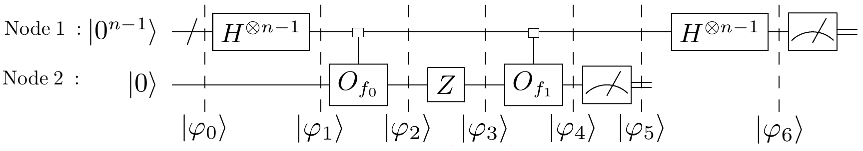
Figure 1: The circuit for the distributed quantum algorithm for DJ problem (two computing nodes) (Algorithm 1 ).

4.2 The correctness analysis of Algorithm 1

In the following, we prove the correctness of Algorithm 1. The state after the first step of Algorithm 1 is:

$$|\varphi_{1}\rangle =\frac{1}{\sqrt{2^{n-1}}}\sum_{u\in\{0,1\}^{n-1}}|u\rangle\ket{0}.$$ (81)

Algorithm 1 then queries the oracle $O_{f_{0}}$, resulting in the following state:

$$\begin{split}|\varphi_{2}\rangle&=O_{f_{0}}|\varphi_{1}\rangle\\ &=\frac{1}{\sqrt{2^{n-1}}}\sum_{u\in\{0,1\}^{n-1}}|u\rangle|f_{0}(u)\rangle\\ \end{split}$$ (82)

Then, the quantum gate $Z$ on $|\varphi_{2}\rangle$ is applied to get the following states:

$$\begin{split}|\varphi_{3}\rangle=&(I\otimes Z)|\varphi_{2}\rangle\\ =&\frac{1}{\sqrt{2^{n-1}}}\sum_{u\in\{0,1\}^{n-1}}(-1)^{f_{0}(u)}|u\rangle|f_{0}(u)\rangle.\end{split}$$ (83)

After applying the operator $O_{f_{1}}$ on $|\varphi_{3}\rangle$, we have the following state:

$$\begin{split}|\varphi_{4}\rangle=&O_{f_{1}}|\varphi_{3}\rangle\\ =&\frac{1}{\sqrt{2^{n-1}}}\sum_{u\in\{0,1\}^{n-1}}(-1)^{f_{0}(u)}|u\rangle|f_{0}(u)\oplus f_{1}(u)\rangle\\ =&\frac{1}{\sqrt{2^{n-1}}}\sum\limits_{\begin{subarray}{c}u\in\{0,1\}^{n-1}\\ f_{0}(u)\oplus f_{1}(u)=0\end{subarray}}(-1)^{f_{0}(u)}|u\rangle\ket{0}+\frac{1}{\sqrt{2^{n-1}}}\sum\limits_{\begin{subarray}{c}u\in\{0,1\}^{n-1}\\ f_{0}(u)\oplus f_{1}(u)=1\end{subarray}}(-1)^{f_{0}(u)}|u\rangle\ket{1}.\end{split}$$ (84)

After measuring on the last qubit of $|\varphi_{4}\rangle$, if the result is $1$, then there $\exists$ $u\in\{0,1\}^{n-1}$ such that $f_{0}(u)\oplus f_{1}(u)=1$. From Corollary 1, we know that $f$ is balanced. If the result is $0$, then we get the state:

$$\begin{split}|\varphi_{5}\rangle=&\frac{1}{\sqrt{M}}\sum\limits_{\begin{subarray}{c}u\in\{0,1\}^{n-1}\\ f_{0}(u)\oplus f_{1}(u)=0\end{subarray}}(-1)^{f_{0}(u)}|u\rangle\ket{0},\\ \end{split}$$ (85)

where $M=|\{u\in\{0,1\}^{n-1}|f_{0}(u)\oplus f_{1}(u)=0\}|$.

After Hadamard transformation on the first $n-1$ qubits of $|\varphi_{5}\rangle$, we obtain the following state:

$$\begin{split}|\varphi_{6}\rangle=&\left(H^{\otimes n-1}\otimes I\right)|\varphi_{5}\rangle\\ =&\frac{1}{\sqrt{2^{n-1}M}}\sum\limits_{\begin{subarray}{c}u,z\in\{0,1\}^{n-1}\\ f_{0}(u)\oplus f_{1}(u)=0\end{subarray}}(-1)^{f_{0}(u)+u\cdot z}\ket{z}\ket{0}.\end{split}$$ (86)

The probability of measuring the first $n-1$ qubits of $|\varphi_{6}\rangle$ with the result of $0^{n-1}$ is

$$\left|\frac{1}{\sqrt{2^{n-1}M}}\sum\limits_{\begin{subarray}{c}u\in\{0,1\}^{n-1}\\ f_{0}(u)\oplus f_{1}(u)=0\end{subarray}}(-1)^{f_{0}(u)}\right|^{2}.$$ (87)

After measuring on the first $n-1$ qubits of $|\varphi_{6}\rangle$, according to Theorem 1, if the result is $0^{n-1}$, then $f$ is constant, otherwise $f$ is balanced.

4.3 Comparison with other algorithms

First, we compare with the distributed quantum algorithm for DJ problem proposed previously [1]. For $t=1$, the algorithm in paper [1] has certain error, but Algorithm 1 can solve it exactly.

Second, we compare with distributed classical deterministic algorithm. Algorithm 1 needs one query for each oracle to solve DJ problem. However, distributed classical deterministic algorithm needs to query oracles $O(2^{n-1})$ times in the worst case. Therefore, Algorithm 1 has the advantage of exponential acceleration compared with the distributed classical deterministic algorithm.

Third, we compare with DJ algorithm. In DJ algorithm, the number of qubits required by the implementation circuit of oracle corresponding to Boolean function $f$ is $n+1$. In Algorithm 1, the number of qubits required by the implementation circuit of oracle corresponding to subfunctions $f_{0}$ and $f_{1}$ is $n$.

Remark 1.

However, Algorithm 1 cannot exactly solve DJ problem in distributed scenario with multiple computing nodes. In D, we give an example to demonstrate that the algorithm cannot exactly solve DJ problem for the case with four computing nodes.

5 Design and analysis of Algorithm 2

Since Algorithm 1 cannot exactly solve DJ problem in distributed scenario with multiple computing nodes, we use the new structural features of DJ problem to design Algorithm 2.

5.1 Design of Algorithm 2

Below we introduce related notation and function that are used in Algorithm 2.

Let $[N]$ represent the set of integers $\{0,1,\cdots,2^{t}-1\}$, ane let $BI:\{0,1\}^{t}\rightarrow[N]$ be the function to convert a binary string of $t$ bits to an equal decimal integer.

Operator $O^{\prime}_{f_{w}}$ in Algorithm 2 is defined as:

$$O^{\prime}_{f_{w}}\ket{u}\ket{b}\ket{c}=\ket{u}\ket{b}\ket{c\oplus f_{w}(u)},$$ (88)

where $w\in\{0,1\}^{t}$, $u\in\{0,1\}^{n-t}$, $b\in\{0,1\}^{BI(w)}$ and $c\in\{0,1\}$.

Operator $U$ in Algorithm 2 is defined as:

$$U\left(\bigotimes_{i\in\{0,1\}^{t}}\ket{a_{i}}\right)|b\rangle=\left(\bigotimes_{i\in\{0,1\}^{t}}\ket{a_{i}}\right)\Ket{b\oplus\left(2^{t}-2\sum\limits_{i\in\{0,1\}^{t}}a_{i}\right)},$$ (89)

where $a_{i}\in\{0,1\}$, $i\in\{0,1\}^{t}$ and $b\in\{0,1\}^{t+2}$. In fact, $U$ is unitary.

Another operator $R$ in Algorithm 2 is defined as:

$$R\ket{d}\ket{e}=\ket{d}\left(\frac{d}{2^{t}}\ket{e}+(-1)^{e}\cdot\sqrt{1-\left(\frac{d}{2^{t}}\right)^{2}}\Ket{1\oplus e}\right),$$ (90)

where $d\in\{0,1\}^{t+2}$ and $e\in\{0,1\}$. Also, $R$ is unitary.

Lemma 1.

The operator $U$ in equation (89) and the operator $R$ in equation (90) are both unitary.

Proof.

Suppose $\left(\bigotimes_{i\in\{0,1\}^{t}}\ket{a_{i}}\right)|b\rangle\neq\left(\bigotimes_{i\in\{0,1\}^{t}}\ket{a^{\prime}_{i}}\right)|b^{\prime}\rangle$. Then

$$\begin{split}&\bra{b^{\prime}}\left(\bigotimes_{i\in\{0,1\}^{t}}\bra{a^{\prime}_{i}}\right)U^{\dagger}U\left(\bigotimes_{i\in\{0,1\}^{t}}\ket{a_{i}}\right)|b\rangle\\ =&\Bra{b^{\prime}\oplus\left(2^{t}-2\sum\limits_{i\in\{0,1\}^{t}}a^{\prime}_{i}\right)}\left(\bigotimes_{i\in\{0,1\}^{t}}\bra{a^{\prime}_{i}}\right)\left(\bigotimes_{i\in\{0,1\}^{t}}\ket{a_{i}}\right)\Ket{b\oplus\left(2^{t}-2\sum\limits_{i\in\{0,1\}^{t}}a_{i}\right)}\\ =&0.\end{split}$$ (91)

Therefore, $U$ is unitary.

Suppose $\ket{d}\ket{e}\neq\ket{d^{\prime}}\ket{e^{\prime}}$. Then

$$\begin{split}&\bra{e^{\prime}}\bra{d^{\prime}}R^{\dagger}R\ket{d}\ket{e}\\ =&\left(\frac{d^{\prime}}{2^{t}}\bra{e^{\prime}}+(-1)^{e^{\prime}}\cdot\sqrt{1-\left(\frac{d^{\prime}}{2^{t}}\right)^{2}}\bra{1\oplus e^{\prime}}\right)\braket{d^{\prime}}{d}\left(\frac{d}{2^{t}}\ket{e}+(-1)^{e}\cdot\sqrt{1-\left(\frac{d}{2^{t}}\right)^{2}}\Ket{1\oplus e}\right)\\ =&0.\end{split}$$ (92)

Therefore, $R$ is unitary. ∎

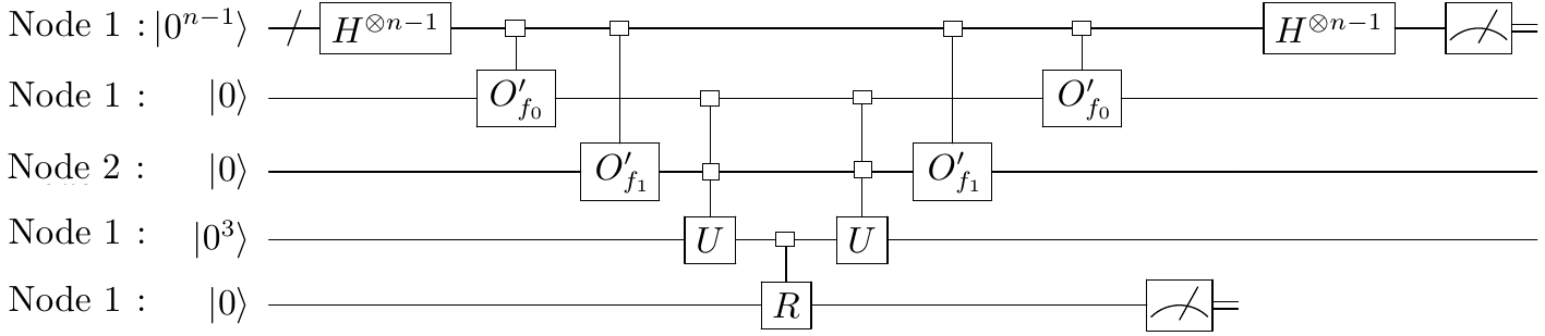
Figure 2: The circuit for the distributed quantum algorithm for DJ problem (two computing nodes) (Algorithm 2 ).

Algorithm 2 Distributed quantum algorithm for DJ problem ($2^{t}$ distributed computing nodes)

1:$\ket{\phi_{0}}=|0^{n-t}\rangle\ket{0^{2^{t}+t+3}}$;

2:$|\phi_{1}\rangle=\left(H^{\otimes n-t}\otimes I^{\otimes{2^{t}+t+3}}\right)\ket{\phi_{0}}$;

3:$\ket{\phi_{2}}=\prod\limits_{w\in\{0,1\}^{t}}\left(O^{\prime}_{f_{w}}\otimes I^{\otimes 2^{t}+t+2-BI(w)}\right)\ket{\phi_{1}}$;

4:$\ket{\phi_{3}}=\left(I^{\otimes{n-t}}\otimes U\otimes I\right)\ket{\phi_{2}}$;

5:$\ket{\phi_{4}}=\left(I^{\otimes{n-t+2^{t}}}\otimes R\right)\ket{\phi_{3}}$;

6:$\ket{\phi_{5}}=\left(\prod\limits_{w\in\{0,1\}^{t}}\left(O^{\prime}_{f_{w}}\otimes I^{\otimes 2^{t}+t+2-BI(w)}\right)\right)\left(I^{\otimes{n-t}}\otimes U\otimes I\right)\ket{\phi_{4}}$;

7:Measure the last qubit of $\ket{\phi_{5}}$: if the result is 1, then output $f$ is balanced; if the result is 0, then denote the quantum state after measurement as $\ket{\phi_{6}}$;

8:$|\phi_{7}\rangle=\left(H^{\otimes n-t}\otimes I^{\otimes{2^{t}+t+3}}\right)|\phi_{6}\rangle$;

9:Measure the first $n-t$ qubits of $\ket{\phi_{7}}$: if the result is $0^{n-t}$, then output $f$ is constant; if the result is not $0^{n-t}$, then output $f$ is balanced.

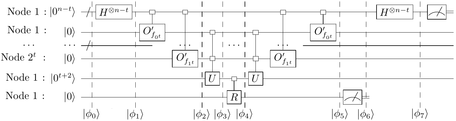
Figure 3: The circuit for the distributed quantum algorithm for DJ problem ($2^{t}$ computing nodes) (Algorithm 2 ).

5.2 Correctness analysis of Algorithm 2

In the following, we prove the correctness of Algorithm 2. The state after the first step of Algorithm 2 is:

$$\begin{split}|\phi_{1}\rangle=&\left(H^{\otimes n-t}\otimes I^{\otimes{2^{t}+t+3}}\right)\ket{\phi_{0}}\\ =&\frac{1}{\sqrt{2^{n-t}}}\sum_{u\in\{0,1\}^{n-t}}|u\rangle\ket{0^{2^{t}+t+3}}.\end{split}$$ (93)

Then Algorithm 2 queries the oracles $O^{\prime}_{f_{w}}$ $\left(w\in\{0,1\}^{t}\right)$, resulting in the following state:

$$\begin{split}|\phi_{2}\rangle=&\prod\limits_{w\in\{0,1\}^{t}}\left(O^{\prime}_{f_{w}}\otimes I^{\otimes 2^{t}+t+2-BI(w)}\right)\ket{\phi_{1}}\\ =&\frac{1}{\sqrt{2^{n-t}}}\sum_{u\in\{0,1\}^{n-t}}|u\rangle\bigotimes\limits_{w\in\{0,1\}^{t}}\ket{f_{w}(u)}|0^{t+3}\rangle.\end{split}$$ (94)

After applying operator $U$, we have the following state:

$$\begin{split}|\phi_{3}\rangle=&\left(I^{\otimes{n-t}}\otimes U\otimes I\right)\ket{\phi_{2}}\\ =&\frac{1}{\sqrt{2^{n-t}}}\sum_{u\in\{0,1\}^{n-t}}|u\rangle\bigotimes\limits_{w\in\{0,1\}^{t}}\ket{f_{w}(u)}\Ket{\delta(u)}\Ket{0},\end{split}$$ (95)

where $\delta(u)=2^{t}-2\sum_{w\in\{0,1\}^{t}}f_{w}(u)$.

After applying operator $R$, we have the following state:

$$\begin{split}|\phi_{4}\rangle=&\left(I^{\otimes{n-t+2^{t}}}\otimes R\right)\ket{\phi_{3}}\\ =&\frac{1}{\sqrt{2^{n-t}}}\sum_{u\in\{0,1\}^{n-t}}|u\rangle\bigotimes\limits_{w\in\{0,1\}^{t}}\ket{f_{w}(u)}\Ket{\delta(u)}\left(\frac{\delta(u)}{2^{t}}\ket{0}+\sqrt{1-\left(\frac{\delta(u)}{2^{t}}\right)^{2}}\ket{1}\right).\end{split}$$ (96)

After applying operator $U$ and $O^{\prime}_{f_{w}}$ $(w\in\{0,1\}^{t})$, resulting in the following state:

$$\begin{split}\ket{\phi_{5}}=&\left(\prod\limits_{w\in\{0,1\}^{t}}\left(O^{\prime}_{f_{w}}\otimes I^{\otimes 2^{t}+t+2-BI(w)}\right)\right)\left(I^{\otimes{n-t}}\otimes U\otimes I\right)\ket{\phi_{4}}\\ =&\frac{1}{\sqrt{2^{n-t}}}\sum_{u\in\{0,1\}^{n-t}}|u\rangle|0^{2^{t}+t+2}\rangle\left(\frac{\delta(u)}{2^{t}}\ket{0}+\sqrt{1-\left(\frac{\delta(u)}{2^{t}}\right)^{2}}\ket{1}\right).\end{split}$$ (97)

After measuring the last qubit of $\ket{\phi_{5}}$, if the result is $1$, then $\exists$ $u\in\{0,1\}^{n-t}$ such that $|\delta(u)|\neq 2^{t}$. From Corollary 2, we know that $f$ is balanced. If the result is $0$, then we get the state:

$$\begin{split}&|\phi_{6}\rangle=\sum_{u\in\{0,1\}^{n-t}}\frac{\delta(u)}{\sqrt{\sum\limits_{u\in\{0,1\}^{n-t}}\delta^{2}(u)}}|u\rangle\ket{0^{2^{t}+t+3}}.\end{split}$$ (98)

With Hadamard transformation on the first $n-t$ qubits of $\ket{\phi_{6}}$, we get the following state:

$$\begin{split}|\phi_{7}\rangle=&\left(H^{\otimes n-t}\otimes I^{\otimes{2^{t}+t+3}}\right)|\phi_{6}\rangle\\ =&\sum_{u,z\in\{0,1\}^{n-t}}\frac{\delta(u)}{\sqrt{\sum\limits_{u\in\{0,1\}^{n-t}}\delta^{2}(u)}}\frac{(-1)^{u\cdot z}}{\sqrt{2^{n-t}}}\ket{z}\ket{0^{2^{t}+t+3}}.\end{split}$$ (99)

The probability of measuring the first $n-t$ qubits of $\ket{\phi_{7}}$ with the result of $0^{n-t}$ is

$$\left|\frac{1}{\sqrt{2^{n-t}\sum\limits_{u\in\{0,1\}^{n-t}}\delta^{2}(u)}}\sum\limits_{u\in\{0,1\}^{n-t}}\delta(u)\right|^{2}.$$ (100)

After measuring the first $n-t$ qubits of $\ket{\phi_{7}}$, according to Theorem 2, if the result is $0^{n-t}$, then $f$ is constant, otherwise $f$ is balanced.

5.3 Comparison with other algorithms

We compare with distributed classical deterministic algorithm. Algorithm 2 needs two queries for each oracle to solve DJ problem. However, distributed classical deterministic algorithm needs to query oracles $O(2^{n-t})$ times in the worst case. Therefore, Algorithm 2 has the advantage of exponential acceleration compared with the distributed classical deterministic algorithm.

Then, we compare with DJ algorithm. In DJ algorithm, the number of qubits required by the implementation circuit of oracle corresponding to Boolean function $f$ is $n+1$. In Algorithm 2, the number of qubits required by the implementation circuit of oracle corresponding to subfunction $f_{w}$ is $n-t+1$.

6 Design and analysis of Algorithm 3

We synthesised the structural features of DJ problem in distributed scenario used in Algorithm 1 and Algorithm 2 to design Algorithm 3. Algorithm 3 combines the design methods and advantages of Algorithm 1 and Algorithm 2, but the number of qubits required to implement certain unitary operators in Algorithm 3 is less than that in Algorithm 2.

6.1 Design of Algorithm 3

In the following, we describe the unitary operators involved in Algorithm 3.

Operator $O^{\prime\prime}_{f_{w^{\prime}0}}$ in Algorithm 3 is defined as:

$$O^{\prime\prime}_{f_{w^{\prime}0}}\ket{u}\ket{b}\ket{c}=\ket{u}\ket{b}\ket{c\oplus f_{w^{\prime}0}(u)},$$ (101)

where $w^{\prime}\in\{0,1\}^{t-1}$, $u\in\{0,1\}^{n-t}$, $b\in\{0,1\}^{3\cdot BI(w^{\prime}0)/2}$ and $c\in\{0,1\}$.

Operator $O^{\prime\prime}_{f_{w^{\prime}1}}$ in Algorithm 3 is defined as:

$$O^{\prime\prime}_{f_{w^{\prime}1}}\ket{u}\ket{b}\ket{c}=\ket{u}\ket{b}\ket{c\oplus f_{w^{\prime}1}(u)},$$ (102)

where $w^{\prime}\in\{0,1\}^{t-1}$, $u\in\{0,1\}^{n-t}$, $b\in\{0,1\}^{3\cdot BI(w^{\prime}0)/2+1}$ and $c\in\{0,1\}$. The function $BI$ is defined in Algorithm 2.

Operator $A$ in Algorithm 3 is defined as:

$$A\left(\bigotimes_{i\in\{0,1\}^{t-1}\setminus\{1^{t-1}\}}\ket{a_{i}}\ket{b}\right)\ket{a_{1^{t-1}}}\ket{c}|d\rangle\\ =\left(\bigotimes_{i\in\{0,1\}^{t-1}\setminus\{1^{t-1}\}}\ket{a_{i}}\ket{b}\right)\ket{a_{1^{t-1}}}\ket{c}\Ket{d\oplus\sum_{i\in\{0,1\}^{t-1}}a_{i}},$$ (103)

where $a_{i}\in\{0,1\}$, $i\in\{0,1\}^{t-1}$, $b\in\{0,1\}^{2}$, $c\in\{0,1\}$ and $d\in\{0,1\}^{t}$.

Operator $V$ in Algorithm 3 is defined as:

$$\begin{split}V\ket{a}\ket{b}\ket{c}=&\ket{a}\ket{b}\Ket{c\oplus\left(2^{t-1}-a-2b\right)},\end{split}$$ (104)

where $a,b\in\{0,1\}^{t}$ and $c\in\{0,1\}^{t+1}$.

Operator $R^{\prime}$ in Algorithm 3 is defined as:

$$R^{\prime}\ket{d}\ket{e}=\ket{d}\left(\frac{d}{2^{t-1}}\ket{e}+(-1)^{e}\cdot\sqrt{1-\left(\frac{d}{2^{t-1}}\right)^{2}}\Ket{1\oplus e}\right),$$ (105)

where $d\in\{0,1\}^{t+1}$ and $e\in\{0,1\}$.

Lemma 2.

The operator $A$ in equation (103), the operator $V$ in equation (104) and the operator $R^{\prime}$ in equation (105) are all unitary.

Proof.

Similar to the proof of Lemma 1. ∎

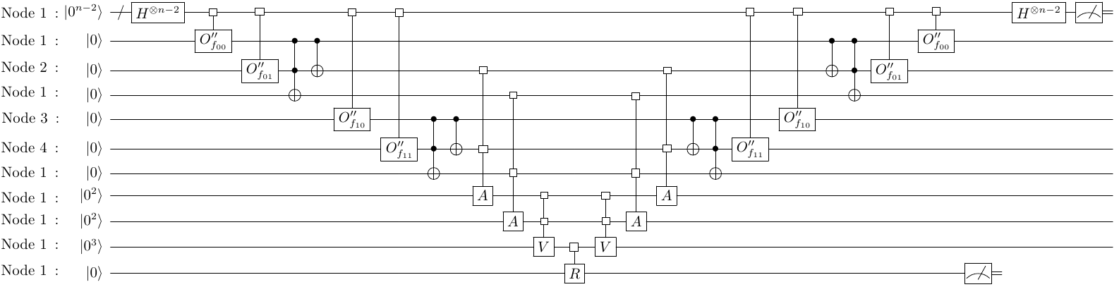
Figure 4: The circuit for the distributed quantum algorithm for DJ problem (four computing nodes) (Algorithm 3 ).

Algorithm 3 Distributed quantum algorithm for DJ problem ($2^{t}$ distributed computing nodes)

1:$|\Phi_{0}\rangle=|0^{n-t}\rangle|0^{3\cdot 2^{t-1}+3t+2}\rangle$;

2:$\ket{\Phi_{1}}=\left(H^{\otimes n-t}\otimes I^{\otimes{3\cdot 2^{t-1}+3t+2}}\right)|\Phi_{0}\rangle$;

3:$|\Phi_{2}\rangle=\prod\limits_{w^{\prime}\in\{0,1\}^{t-1}}\left[\left(I^{\otimes n-t+3\cdot BI(w^{\prime}0)/2}\otimes{\rm CNOT}\otimes I^{\otimes 3\cdot 2^{t-1}+3t-3\cdot BI(w^{\prime}0)/2}\right)\right.$ $\quad\left(I^{\otimes n-t+3\cdot BI(w^{\prime}0)/2}\otimes{\rm CCNOT}\otimes I^{\otimes 3\cdot 2^{t-1}+3t-3\cdot BI(w^{\prime}0)/2-1}\right)$ $\quad\left.\left(O^{\prime\prime}_{f_{w^{\prime}1}}\otimes I^{\otimes 3\cdot 2^{t-1}+3t-3\cdot BI(w^{\prime}0)/2}\right)\left(O^{\prime\prime}_{f_{w^{\prime}0}}\otimes I^{\otimes 3\cdot 2^{t-1}+3t-3\cdot BI(w^{\prime}0)/2+1}\right)\right]\ket{\Phi_{1}}$

4:$|\Phi_{3}\rangle=\prod\limits_{i=1}^{2}\left(I^{\otimes n-t+i}\otimes A\otimes I^{\otimes(3-i)t+2}\right)\ket{\Phi_{2}}$;

5:$\Ket{\Phi_{4}}=\left(I^{\otimes n-t+3\cdot 2^{t-1}}\otimes V\otimes I\right)\Ket{\Phi_{3}}$;

6:$\Ket{\Phi_{5}}=\left(I^{\otimes n+3\cdot 2^{t-1}+t}\otimes R^{\prime}\right)\Ket{\Phi_{4}}$;

7:$\ket{\Phi_{6}}=\prod\limits_{w^{\prime}\in\{0,1\}^{t-1}}\left[\left(I^{\otimes n-t+3\cdot BI(w^{\prime}0)/2}\otimes{\rm CNOT}\otimes I^{\otimes 3\cdot 2^{t-1}+3t-3\cdot BI(w^{\prime}0)/2}\right)\right.$ $\quad\left(I^{\otimes n-t+3\cdot BI(w^{\prime}0)/2}\otimes{\rm CCNOT}\otimes I^{\otimes 3\cdot 2^{t-1}+3t-3\cdot BI(w^{\prime}0)/2-1}\right)$ $\quad\left.\left(O^{\prime\prime}_{f_{w^{\prime}1}}\otimes I^{\otimes 3\cdot 2^{t-1}+3t-3\cdot BI(w^{\prime}0)/2}\right)\left(O^{\prime\prime}_{f_{w^{\prime}0}}\otimes I^{\otimes 3\cdot 2^{t-1}+3t-3\cdot BI(w^{\prime}0)/2+1}\right)\right]$ $\quad\prod\limits_{i=1}^{2}\left(I^{\otimes n-t+i}\otimes A\otimes I^{\otimes(3-i)t+2}\right)\left(I^{\otimes n-t+3\cdot 2^{t-1}}\otimes V\otimes I\right)\ket{\Phi_{5}}$;

8:Measure the last qubit of $\ket{\Phi_{6}}$: if the result is 1, then output $f$ is balanced; if the result is 0, then denote the quantum state after measurement as $\ket{\Phi_{7}}$;

9:$|\Phi_{8}\rangle=\left(H^{\otimes n-t}\otimes I^{\otimes{3\cdot 2^{t-1}+3t+2}}\right)|\Phi_{7}\rangle$;

10:Measure the first $n-t$ qubits of $\ket{\Phi_{8}}$: if the result is $0^{n-t}$, then output $f$ is constant; if the result is not $0^{n-t}$, then output $f$ is balanced.

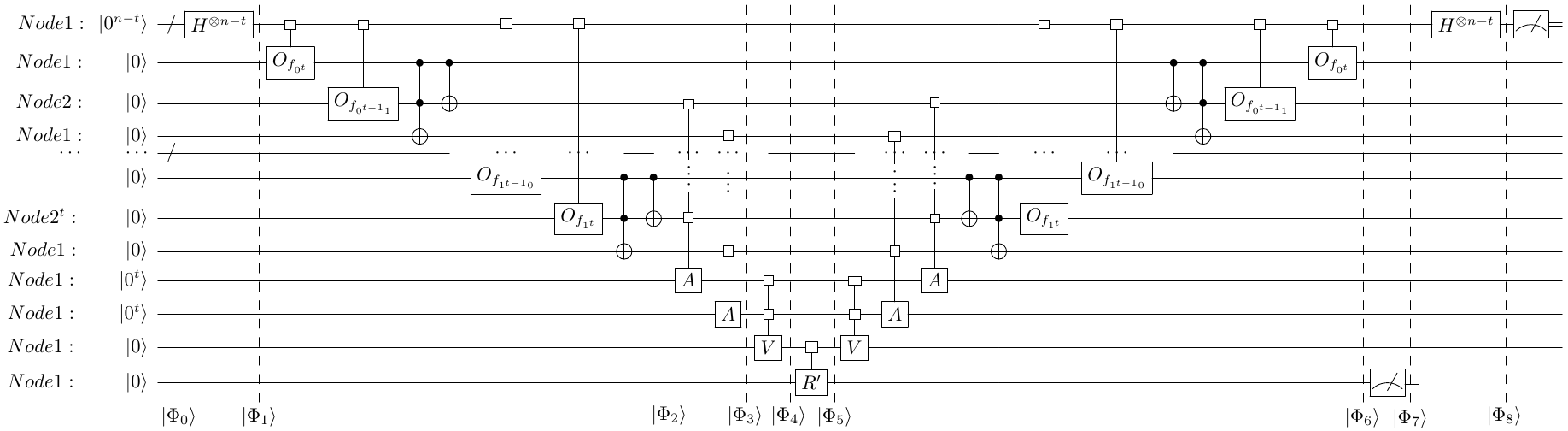
Figure 5: The circuit for the distributed quantum algorithm for DJ problem ($2^{t}$ computing nodes) (Algorithm 3 ).

6.2 Correctness analysis of Algorithm 3

In the following, we prove the correctness of Algorithm 3. The state after the first step of Algorithm 3 is:

$$\begin{split}\ket{\Phi_{1}}=&\left(H^{\otimes n-t}\otimes I^{\otimes{3\cdot 2^{t-1}+3t+2}}\right)|\Phi_{0}\rangle\\ =&\frac{1}{\sqrt{2^{n-t}}}\sum_{u\in\{0,1\}^{n-t}}|u\rangle\ket{0^{3\cdot 2^{t-1}+3t+2}}.\end{split}$$ (106)

Then Algorithm 3 queries the oracles $O^{\prime\prime}_{f_{w^{\prime}0}}$ and $O^{\prime\prime}_{f_{w^{\prime}1}}$ $(w^{\prime}\in\{0,1\}^{t-1})$, and applies the operators ${\rm CCNOT}$ and ${\rm CNOT}$, resulting in the following state:

$$\begin{split}|\Phi_{2}\rangle=&\prod\limits_{w^{\prime}\in\{0,1\}^{t-1}}\left[\left(I^{\otimes n-t+3\cdot BI(w^{\prime}0)/2}\otimes{\rm CNOT}\otimes I^{\otimes 3\cdot 2^{t-1}+3t-3\cdot BI(w^{\prime}0)/2}\right)\right.\\ &\left(I^{\otimes n-t+3\cdot BI(w^{\prime}0)/2}\otimes{\rm CCNOT}\otimes I^{\otimes 3\cdot 2^{t-1}+3t-3\cdot BI(w^{\prime}0)/2-1}\right)\\ &\left.\left(O^{\prime\prime}_{f_{w^{\prime}1}}\otimes I^{\otimes 3\cdot 2^{t-1}+3t-3\cdot BI(w^{\prime}0)/2}\right)\left(O^{\prime\prime}_{f_{w^{\prime}0}}\otimes I^{\otimes 3\cdot 2^{t-1}+3t-3\cdot BI(w^{\prime}0)/2+1}\right)\right]\ket{\Phi_{1}}\\ =&\frac{1}{\sqrt{2^{n-t}}}\sum_{u\in\{0,1\}^{n-t}}|u\rangle\left(\bigotimes_{w^{\prime}\in\{0,1\}^{t-1}}|f_{w^{\prime}0}(u)\rangle|f_{w^{\prime}0}(u)\oplus f_{w^{\prime}1}(u)\rangle|f_{w^{\prime}0}(u)\land f_{w^{\prime}1}(u)\rangle\right)\ket{0^{3t+2}}.\end{split}$$ (107)

By applying the operator $A$ on $\ket{\Phi_{2}}$, we obtain the following state:

$$\begin{split}|\Phi_{3}\rangle=&\prod\limits_{i=1}^{2}\left(I^{\otimes n-t+i}\otimes A\otimes I^{\otimes(3-i)t+2}\right)\ket{\Phi_{2}}\\ =&\frac{1}{\sqrt{2^{n-t}}}\sum_{u\in\{0,1\}^{n-t}}|u\rangle\left(\bigotimes_{w^{\prime}\in\{0,1\}^{t-1}}|f_{w^{\prime}0}(u)\rangle|f_{w^{\prime}0}(u)\oplus f_{w^{\prime}1}(u)\rangle|f_{w^{\prime}0}(u)\land f_{w^{\prime}1}(u)\rangle\right)\\ &\left|\sum_{w^{\prime}\in\{0,1\}^{t-1}}f_{w^{\prime}0}(u)\oplus f_{w^{\prime}1}(u)\right\rangle\Ket{\sum_{w^{\prime}\in\{0,1\}^{t-1}}f_{w^{\prime}0}(u)\land f_{w^{\prime}1}(u)}\Ket{0^{t+2}}.\end{split}$$ (108)

By applying the operator $V$ on $\ket{\Phi_{3}}$, we get the following state:

$$\begin{split}\Ket{\Phi_{4}}=&\left(I^{\otimes n-t+3\cdot 2^{t-1}}\otimes V\otimes I\right)\Ket{\Phi_{3}}\\ =&\frac{1}{\sqrt{2^{n-t}}}\sum_{u\in\{0,1\}^{n-t}}|u\rangle\left(\bigotimes_{w^{\prime}\in\{0,1\}^{t-1}}|f_{w^{\prime}0}(u)\rangle|f_{w^{\prime}0}(u)\oplus f_{w^{\prime}1}(u)\rangle|f_{w^{\prime}0}(u)\land f_{w^{\prime}1}(u)\rangle\right)\\ &\left|\sum_{w^{\prime}\in\{0,1\}^{t-1}}f_{w^{\prime}0}(u)\oplus f_{w^{\prime}1}(u)\right\rangle\Ket{\sum_{w^{\prime}\in\{0,1\}^{t-1}}f_{w^{\prime}0}(u)\land f_{w^{\prime}1}(u)}\Ket{\Delta(u)}\Ket{0},\end{split}$$ (109)

where $\Delta(u)=2^{t-1}-\sum_{w^{\prime}\in\{0,1\}^{t-1}}f_{w^{\prime}0}(u)\oplus f_{w^{\prime}1}(u)-2\sum_{w^{\prime}\in\{0,1\}^{t-1}}f_{w^{\prime}0}(u)\land f_{w^{\prime}1}(u)$.

Then we apply the operator $R^{\prime}$ on $\Ket{\Phi_{4}}$, and the following state is obtained:

$$\begin{split}\Ket{\Phi_{5}}=&\left(I^{\otimes n+3\cdot 2^{t-1}+t}\otimes R^{\prime}\right)\Ket{\Phi_{4}}\\ =&\frac{1}{\sqrt{2^{n-t}}}\sum_{u\in\{0,1\}^{n-t}}|u\rangle\left(\bigotimes_{w^{\prime}\in\{0,1\}^{t-1}}|f_{w^{\prime}0}(u)\rangle|f_{w^{\prime}0}(u)\oplus f_{w^{\prime}1}(u)\rangle|f_{w^{\prime}0}(u)\land f_{w^{\prime}1}(u)\rangle\right)\\ &\left|\sum_{w^{\prime}\in\{0,1\}^{t-1}}f_{w^{\prime}0}(u)\oplus f_{w^{\prime}1}(u)\right\rangle\Ket{\sum_{w^{\prime}\in\{0,1\}^{t-1}}f_{w^{\prime}0}(u)\land f_{w^{\prime}1}(u)}\Ket{\Delta(u)}\\ &\left(\frac{\Delta(u)}{2^{t-1}}\ket{0}+\sqrt{1-\left(\frac{\Delta(u)}{2^{t-1}}\right)^{2}}\ket{1}\right).\end{split}$$ (110)

In addition, we restore the middle $3\cdot 2^{t-1}+3t+1$ qubits of $\Ket{\Phi_{5}}$ to $\Ket{0^{3\cdot 2^{t-1}+3t+1}}$, resulting in the following state:

$$\begin{split}\ket{\Phi_{6}}=&\prod\limits_{w^{\prime}\in\{0,1\}^{t-1}}\left[\left(I^{\otimes n-t+3\cdot BI(w^{\prime}0)/2}\otimes{\rm CNOT}\otimes I^{\otimes 3\cdot 2^{t-1}+3t-3\cdot BI(w^{\prime}0)/2}\right)\right.\\ &\left(I^{\otimes n-t+3\cdot BI(w^{\prime}0)/2}\otimes{\rm CCNOT}\otimes I^{\otimes 3\cdot 2^{t-1}+3t-3\cdot BI(w^{\prime}0)/2-1}\right)\\ &\left.\left(O^{\prime\prime}_{f_{w^{\prime}1}}\otimes I^{\otimes 3\cdot 2^{t-1}+3t-3\cdot BI(w^{\prime}0)/2}\right)\left(O^{\prime\prime}_{f_{w^{\prime}0}}\otimes I^{\otimes 3\cdot 2^{t-1}+3t-3\cdot BI(w^{\prime}0)/2+1}\right)\right]\\ &\quad\prod\limits_{i=1}^{2}\left(I^{\otimes n-t+i}\otimes A\otimes I^{\otimes(3-i)t+2}\right)\left(I^{\otimes n-t+3\cdot 2^{t-1}}\otimes V\otimes I\right)\ket{\Phi_{5}}\\ =&\frac{1}{\sqrt{2^{n-t}}}\sum_{u\in\{0,1\}^{n-t}}|u\rangle\Ket{0^{3\cdot 2^{t-1}+3t+1}}\left(\frac{\Delta(u)}{2^{t-1}}\ket{0}+\sqrt{1-\left(\frac{\Delta(u)}{2^{t-1}}\right)^{2}}\ket{1}\right).\end{split}$$ (111)

After measurement on the last qubit of $\ket{\Phi_{6}}$, if the result is $1$, then $\exists$ $u\in\{0,1\}^{n-t}$ such that $|\Delta(u)|\neq 2^{t-1}$. From Corollary 3, we know that $f$ is balanced. If the result is $0$, then we get the state:

$$\begin{split}|\Phi_{7}\rangle=\sum_{u\in\{0,1\}^{n-t}}\frac{\Delta(u)}{\sqrt{\sum\limits_{u\in\{0,1\}^{n-t}}\Delta^{2}(u)}}|u\rangle\ket{0^{3\cdot 2^{t-1}+3t+2}}.\end{split}$$ (112)

By using Hadamard transformation on the first $n-t$ qubits of $\ket{\Phi_{7}}$, we get the following state:

$$\begin{split}|\Phi_{8}\rangle=&\left(H^{\otimes n-t}\otimes I^{\otimes{3\cdot 2^{t-1}+3t+2}}\right)|\Phi_{7}\rangle\\ =&\sum_{u,z\in\{0,1\}^{n-t}}\frac{\Delta(u)}{\sqrt{\sum\limits_{u\in\{0,1\}^{n-t}}\Delta^{2}(u)}}\frac{(-1)^{u\cdot z}}{\sqrt{2^{n-t}}}\ket{z}\ket{0^{3\cdot 2^{t-1}+3t+2}}.\end{split}$$ (113)

The probability of measuring the first $n-t$ qubits of $\ket{\Phi_{8}}$ with the result of $0^{n-t}$ is

$$\left|\frac{1}{\sqrt{2^{n-t}\sum\limits_{u\in\{0,1\}^{n-t}}\Delta^{2}(u)}}\sum\limits_{u\in\{0,1\}^{n-t}}\Delta(u)\right|^{2}.$$ (114)

After measurement on the first $n-t$ qubits of $\ket{\Phi_{8}}$, according to Theorem 3, if the result is $0^{n-t}$, then $f$ is constant, otherwise $f$ is balanced.

6.3 Comparison with other algorithms

Actually, the comparisons of Algorithm 3 with the distributed quantum algorithm for DJ problem proposed previously [1], distributed classical deterministic algorithm, and DJ algorithm are the same as that of Algorithm 2.

In the following, we analyze and compare the three algorithms we designed. Compared Algorithm 1 with Algorithm 2, Algorithm 1 has the advantage that the number of quantum gates and qubits required by the circuit is reduced. Algorithm 2 has the advantage of scaling to multiple computing nodes.

Compared Algorithm 2 with Algorithm 3, Algorithm 2 has the advantage of fewer total qubits and quantum gates. Algorithm 3 has the advantage that the qubit number for realizing some single unitary operators decreases. For instance, the number of qubits required for the unitary operator $V$ in Algorithm 3 is $3t+1$, while the number of qubits required for the unitary operator $U$ in Algorithm 2 is $2^{t}+t+2$.

Although the number of qubits required for the unitary operator $A$ in Algorithm 3 is $3\cdot 2^{t-1}+t-1$, actually, with the help of auxiliary $2^{t-1}$ qubits, we can put the $2^{t-1}$ control qubits $\ket{a_{i}}$ of the operator $A$ together by teleportation, and replace the operator $A$ with the operator $A^{\prime}$, the operator $A^{\prime}$ is defined as:

$$A^{\prime}\left(\bigotimes_{i\in\{0,1\}^{t-1}}\ket{a_{i}}\right)|d\rangle\\ =\left(\bigotimes_{i\in\{0,1\}^{t-1}}\ket{a_{i}}\right)\Ket{d\oplus\sum_{i\in\{0,1\}^{t-1}}a_{i}},$$ (115)

where $\forall a_{i}\in\{0,1\}$, $i\in\{0,1\}^{t-1}$ and $d\in\{0,1\}^{t}$. It is clear that the qubit number of $A^{\prime}$ is $2^{t-1}+t$, which is less than the qubit number of $A$ in Algorithm 3 and qubit number of $U$ in Algorithm 2.

The performance of our algorithms is shown in TAB. 1.

	Total number of qubits	Number of quantum gates	The number of qubits of a single unitary operator
Algorithm 1	$n$	5	The qubit number of $Z$ is $1$
Algorithm 2	$n+2^{t}+3$	$2^{t+1}+6$	The qubit number of $U$ is $2^{t}+t+2$ The qubit number of $R$ is $t+3$
Algorithm 3	$n+3\cdot 2^{t-1}+2t+2$	$2^{t+2}+10$	The qubit number of $A$ is $3\cdot 2^{t-1}+t-1$ The qubit number of $V$ is $3t+1$ The qubit number of $R^{\prime}$ is $t+2$

Table 1: The performance table of our algorithms.

7 Concluding remarks

In comparsion to quantum algorithms, dsitributed quantum algorithms usually have the advantages of less number of input qubits and circuit depth [1, 2, 5, 12, 15, 20, 21], and this subject is therefore important and practical. However, for designing efficient distributed quantum algorithms, the structure of problem to be solved should be clarified in distributed framework.

In this paper, we have discovered the essential structure of DJ problem in distributed scenario by presenting a number of equivalence characterizations between a DJ problem being constant (balanced) and the properties of its subfunctions. These structure properties have provided fundamental ideas for designing distributed exact DJ algorithms. If these structure properties are ignored and we just use DJ algorithm to solve each subfunction, then the result is not exact and the error will be higher and higher with the increasing of number of subfunctions.

By using the structure properties of DJ problem in distributed situation, we have designed three distributed exact quantum algorithms for solving DJ problem, that is, Algorithm 1, Algorithm 2 and Algorithm 3. Algorithm 1 can only solve DJ problem in distributed condition with two subfunctions. So, we have designed Algorithm 2, and it can solve DJ problem in distributed situation with multiple subfunctions.

By combining the ideas and methods of Algorithm 1 and Algorithm 2, we have further given Algorithm 3, which also can solve DJ problem in distributed situation with multiple computing nodes, and some of its single quantum gates require less qubits than Algorithm 2.

These distributed exact DJ algorithms we have designed have the following advantages. First, compared with distributed classical deterministic algorithm, our algorithms have exponential advantage in query complexity; second, compared with DJ algorithm, the single query operator in our algorithms requires fewer qubits, and the depth of circuit is reduced [2], which has better anti-noise performance.

By the way, since each oracle in Algorithm 2 and Algorithm 3 is controlled by the same set of control bits and is serially connected, Algorithm 2 and Algorithm 3 are serial quantum query algorithms. In fact, the oracle query of each computing node in Algorithm 2 and Algorithm 3 can be completed in parallel. With the help of auxiliary $\left(2^{t}-1\right)\left(n-t\right)$ qubits, we can change the state (i.e. $\dfrac{1}{\sqrt{2^{n-t}}}\sum_{u\in\{0,1\}^{n-t}}|u\rangle$) of the control register after the first Hadamard transformation to $\dfrac{1}{\sqrt{2^{n-t}}}\sum_{u\in\{0,1\}^{n-t}}\underbrace{|u\rangle|u\rangle\ldots|u\rangle}_{2^{t}}$. That is to say, we can change the control register from one group to the same $2^{t}$ groups.

More exactly, after the first Hadamard transformation, we can teleport each group of $n-t$ control qubits to every computing node and use these to control the oracles of the computing nodes. By teleporting control qubits, we can replace $O^{\prime}_{f_{w}}$ in Algorithm 2 and $O^{\prime\prime}_{f_{w}}$ in Algorithm 3 by $O_{f_{w}}$.

It is clear that in general the number of qubits needed for $O_{f_{w}}$ is $n-t+1$, which is less than those for $O^{\prime}_{f_{w}}$ and $O^{\prime\prime}_{f_{w}}$, due to the fact that $O_{f_{w}}$ does not necessarily have to cross the line. Therefore, using quantum teleportation to transmit control bits would not only change Algorithm 2 and Algorithm 3 to parallel quantum query algorithms, but also reduce the number of qubits required for each of their oracles. However, the use of quantum teleportation may increase the communication complexity of algorithms.

In sequential researches, we would like to study distributed quantum algorithms for solving generalized DJ problem, generalized Simon problem, and other hidden group problems.

Appendix A DJ Algorithm

Algorithm 4 DJ algorithm

1:$|\psi_{0}\rangle=|0\rangle^{\otimes n}|1\rangle$;

2:$|\psi_{1}\rangle=H^{\otimes n+1}|\psi_{0}\rangle=\frac{1}{\sqrt{2^{n}}}\sum\limits_{x\in\{0,1\}^{n}}|x\rangle|-\rangle$;

3:$|\psi_{2}\rangle=O_{f}|\psi_{1}\rangle=\frac{1}{\sqrt{2^{n}}}\sum\limits_{x\in\{0,1\}^{n}}|x\rangle\Big{(}\frac{|0\oplus f(x)\rangle-|1\oplus f(x)\rangle}{\sqrt{2}}\Big{)}=\frac{1}{\sqrt{2^{n}}}\sum\limits_{x\in\{0,1\}^{n}}(-1)^{f(x)}|x\rangle|-\rangle$;

4:$|\psi_{3}\rangle=H^{\otimes n+1}|\psi_{2}\rangle=\sum\limits_{x,z\in\{0,1\}^{n}}\dfrac{(-1)^{x\cdot z+f(x)}}{2^{n}}|z\rangle|1\rangle$;

5:Measure the first $n$ qubits of $\ket{\psi_{3}}$: if the result is not $0^{n}$, then output $f$ is balanced; if the result is $0^{n}$, then output $f$ is constant.

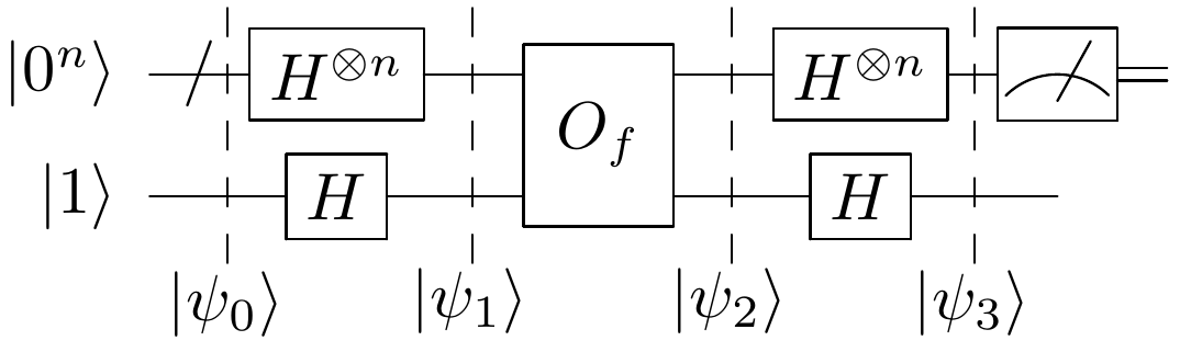
Figure 6: The circuit for DJ algorithm (Algorithm 4 ).

Appendix B Distributed DJ algorithm for multiple computing nodes with errors

In the following, we first give the algorithm ${\rm DJ}_{w}$ that acts on subfunction $f_{w}$.

Algorithm 5 ${\rm DJ}_{w}$ algorithm

1:$|\psi^{\prime}_{0}\rangle=|0^{n-t}\rangle|1\rangle$;

2:$|\psi^{\prime}_{1}\rangle=H^{\otimes n-t+1}|\psi^{\prime}_{0}\rangle=\frac{1}{\sqrt{2^{n-t}}}\sum\limits_{x\in\{0,1\}^{n-t}}|x\rangle|-\rangle$;

3:$|\psi^{\prime}_{2}\rangle=O_{f_{w}}|\psi^{\prime}_{1}\rangle=\frac{1}{\sqrt{2^{n-t}}}\sum\limits_{x\in\{0,1\}^{n-t}}(-1)^{f_{w}(u)}|x\rangle|-\rangle$;

4:$|\psi^{\prime}_{3}\rangle=H^{\otimes n-t+1}|\psi^{\prime}_{2}\rangle=\sum\limits_{x,z\in\{0,1\}^{n-t}}\dfrac{(-1)^{x\cdot z+f_{w}(u)}}{2^{n-t}}|z\rangle|1\rangle$;

5:Measure the first $n-t$ qubits of $\ket{\psi^{\prime}_{3}}$: if the result is not $0^{n-t}$, then output $f_{w}$ is not constant; if the result is $0^{n-t}$, then output $f_{w}$ is not balanced.

Figure 7: The circuit for ${\rm DJ}_{w}$ algorithm (Algorithm 5 ).

In the following, we design Algorithm 6, which generalizes the algorithm in [1] .

Algorithm 6 Distributed DJ algorithm for multiple computing nodes with errors

1:Decompose Boolean function $f:\{0,1\}^{n}\rightarrow\{0,1\}$ into $2^{t}$ subfunctions $f_{w}$ $(w\in\{0,1\}^{t})$ as Equation (9);

2:Apply the ${\rm DJ}_{w}$ algorithm to subfunction $f_{w}$;

3:Record the measurement result of ${\rm DJ}_{w}$ algorithm as $M_{w}$;

4:If there is $M_{w}$ that is not $0^{n-t}$, then output $f$ is balanced;

5:If all $M_{w}$ are $0^{n-t}$, then output $f$ is constant.

In the following, we give the error analysis for Algorithm 6.

Let $l_{w}=|\{u\in\{0,1\}^{n-t}|f_{w}(u)=1\}|$, where $w\in\{0,1\}^{t}$.

The probability that $M_{w}=0^{n-t}$ in the case $l_{w}=k_{w}$ is

$$\begin{split}&\Pr(M_{w}=0^{n-t}|l_{w}=k_{w})\\ =&\left|\frac{1}{2^{n-t}}[k_{w}\cdot(-1)+(2^{n-t}-k_{w})\cdot 1]\right|^{2}\\ =&\left(\dfrac{2^{t+1}}{N}k_{w}-1\right)^{2}.\end{split}$$ (116)

The probability that Algorithm 6 misidentifies a balanced function as constant is

$$\begin{split}&\Pr(f\ is\ \ balanced,M_{w}=0^{n-t},\forall w\in\{0,1\}^{t})\\ =&\sum\limits_{\begin{subarray}{c}\sum\limits_{w\in\{0,1\}^{t}}k_{w}=\frac{N}{2}\\ 0\leq k_{w}\leq\frac{N}{2^{t}}\end{subarray}}\Pr(l_{w}=k_{w})\Pr(M_{w}=0^{n-t},\forall w\in\{0,1\}^{t}|l_{w}=k_{w})\\ =&\sum\limits_{\begin{subarray}{c}\sum\limits_{w\in\{0,1\}^{t}}k_{w}=\frac{N}{2}\\ 0\leq k_{w}\leq\frac{N}{2^{t}}\\ \end{subarray}}\frac{\dbinom{N/2^{t}}{k_{0}}\dbinom{N/2^{t}}{k_{1}}\cdots\dbinom{N/2^{t}}{k_{2^{t}-1}}}{\dbinom{N}{N/2}}\prod\limits_{w\in\{0,1\}^{t}}\left(\dfrac{2^{t+1}}{N}k_{w}-1\right)^{2}.\\ >0.\end{split}$$ (117)

Although the algorithm in [1] can be extended to the general case of multiple distributed computing nodes, i.e. Algorithm 6, it follows from equation 117 that the probability that Algorithm 6 misidentifies a balanced function as constant is at least $0$.

Appendix C Examples of the structure of DJ problem in distributed scenario

Example 1.

Given a Boolean function $f:\{0,1\}^{3}\rightarrow\{0,1\}$ for DJ problem, decompose $f$ into two subfunctions: $f_{0}$ and $f_{1}$, which are assumed to be as follows.

	0	1
00	1	0
01	0	0
10	0	1
11	1	1

Table 2: Example of the structured table for DJ problem in distributed scenario with two subfunctions

It is clear that

$$B_{00}= |\{u\in\{0,1\}^{2}|f_{0}(u)=f_{1}(u)=0\}|=1.$$ (118)

$$B_{11}= |\{u\in\{0,1\}^{2}|f_{0}(u)=f_{1}(u)=1\}|=1.$$ (119)

$$M= |\{u\in\{0,1\}^{2}|f_{0}(u)\oplus f_{1}(u)=0\}|=2.$$ (120)

Therefore

$$B_{00}=B_{11}=M/2.$$ (121)

From Theorem 1, we can deduce that $f$ is balanced.

Example 2.

Given a Boolean function $f:\{0,1\}^{4}\rightarrow\{0,1\}$ for DJ problem, decompose $f$ into four subfunctions: $f_{00}$, $f_{01}$, $f_{10}$ and $f_{11}$, which are assumed to be as follows.

	00	01	10	11
00	1	0	1	0
01	1	0	1	1
10	0	1	0	0
11	1	1	0	0

Table 3: Example of the structured table for DJ problem in distributed scenario with four subfunctions

It is clear that

$$\delta(00)=0;\ \delta(01)=-2;\ \delta(10)=2;\ \delta(11)=0.$$ (122)

Therefore

$$\sum\limits_{u\in\{0,1\}^{2}}\delta(u)=0.$$ (123)

From Theorem 2, we can deduce that $f$ is balanced.

Example 3.

Given a Boolean function $f:\{0,1\}^{4}\rightarrow\{0,1\}$ for DJ problem, decompose $f$ into four subfunctions: $f_{00}$, $f_{01}$, $f_{10}$ and $f_{11}$, which are assumed to be as follows.

	00	01	10	11
00	1	1	0	0
01	1	0	1	1
10	0	1	0	0
11	1	0	1	0

Table 4: Example of the structured table for DJ problem in distributed scenario with four subfunctions

It is clear that

$$\Delta(00)=0;\ \Delta(01)=-1;\ \Delta(10)=1;\ \Delta(11)=0.$$ (124)

Therefore

$$\sum\limits_{u\in\{0,1\}^{2}}\Delta(u)=0.$$ (125)

From Theorem 3, we can deduce that $f$ is balanced.

Appendix D Distributed quantum algorithm for DJ problem with errors (four distributed computing nodes)

Algorithm 7 Distributed quantum algorithm for DJ problem with errors (four distributed computing nodes)

1:$|\varphi^{\prime}_{0}\rangle=|0^{n-2}\rangle\ket{0^{n-2}}$;

2:$|\varphi^{\prime}_{1}\rangle=\left(H^{\otimes n-2}\otimes I\right)|\psi^{\prime}_{0}\rangle$;

3:$|\varphi^{\prime}_{2}\rangle=O_{f_{01}}O_{f_{00}}|\varphi^{\prime}_{1}\rangle$;

4:$|\varphi^{\prime}_{3}\rangle=(I\otimes Z)|\varphi^{\prime}_{2}\rangle$;

5:$|\varphi^{\prime}_{4}\rangle=O_{f_{11}}O_{f_{10}}|\varphi^{\prime}_{3}\rangle$;

6:Measure the last qubit of $|\varphi^{\prime}_{4}\rangle$: if the result is 1, then output $f$ is balanced; if the result is 0, then denote the quantum state after measurement as $\ket{\varphi^{\prime}_{5}}$;

7:$|\varphi^{\prime}_{6}\rangle=\left(H^{\otimes n-2}\otimes I\right)|\varphi^{\prime}_{5}\rangle$;

8:Measure the first $n-2$ qubits of $\ket{\varphi^{\prime}_{6}}$: if the result is not $0^{n-2}$, then output $f$ is balanced; if the result is $0^{n-2}$, then output $f$ is constant.

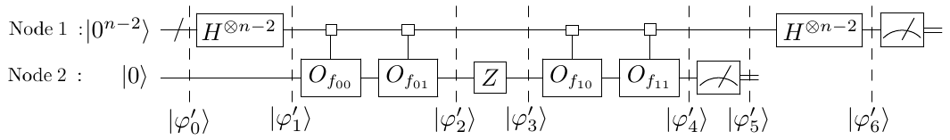
Figure 8: The circuit for the distributed quantum algorithm for DJ problem with errors (four computing nodes) (Algorithm 7 ).

In the following, we prove that Algorithm 7 is not exact and has error. The state after the first step of Algorithm 7 is:

$$|\varphi^{\prime}_{1}\rangle =\frac{1}{\sqrt{2^{n-2}}}\sum_{u\in\{0,1\}^{n-2}}|u\rangle\ket{0}.$$ (126)

Algorithm 7 then queries the oracle $O_{f_{00}}$ and the oracle $O_{f_{01}}$, resulting in the following state:

$$\begin{split}|\varphi^{\prime}_{2}\rangle&=O_{f_{01}}O_{f_{00}}|\varphi^{\prime}_{1}\rangle\\ &=\frac{1}{\sqrt{2^{n-2}}}\sum_{u\in\{0,1\}^{n-2}}|u\rangle|f_{00}(u)\oplus f_{01}(u)\rangle\\ \end{split}$$ (127)

Then, the quantum gate $Z$ on $|\varphi^{\prime}_{2}\rangle$ is applied to get the following states:

$$\begin{split}|\varphi^{\prime}_{3}\rangle=&(I\otimes Z)|\varphi^{\prime}_{2}\rangle\\ =&\frac{1}{\sqrt{2^{n-2}}}\sum_{u\in\{0,1\}^{n-2}}(-1)^{f_{00}(u)\oplus f_{01}(u)}|u\rangle|f_{00}(u)\oplus f_{01}(u)\rangle.\end{split}$$ (128)

After applying the operator $O_{f_{10}}$ and $O_{f_{11}}$ on $|\varphi^{\prime}_{3}\rangle$, we have the following state:

$$\begin{split}|\varphi^{\prime}_{4}\rangle=&O_{f_{11}}O_{f_{10}}|\varphi^{\prime}_{3}\rangle\\ =&\frac{1}{\sqrt{2^{n-2}}}\sum_{u\in\{0,1\}^{n-2}}(-1)^{f_{00}(u)\oplus f_{01}(u)}|u\rangle|f_{00}(u)\oplus f_{01}(u)\oplus f_{10}(u)\oplus f_{11}(u)\rangle\\ =&\frac{1}{\sqrt{2^{n-2}}}\sum\limits_{\begin{subarray}{c}u\in\{0,1\}^{n-2}\\ f_{00}(u)\oplus f_{01}(u)\oplus f_{10}(u)\oplus f_{11}(u)=0\end{subarray}}(-1)^{f_{00}(u)\oplus f_{01}(u)}|u\rangle\ket{0}\\ &+\frac{1}{\sqrt{2^{n-2}}}\sum\limits_{\begin{subarray}{c}u\in\{0,1\}^{n-2}\\ f_{00}(u)\oplus f_{01}(u)\oplus f_{10}(u)\oplus f_{11}(u)=1\end{subarray}}(-1)^{f_{00}(u)\oplus f_{01}(u)}|u\rangle\ket{1}.\end{split}$$ (129)

After measuring on the last qubit of $|\varphi^{\prime}_{4}\rangle$, if the result is $1$, then there $\exists$ $u\in\{0,1\}^{n-2}$ such that $f(u00)\oplus f(u01)\oplus f(u11)\oplus f(u10)=1$. Similar to the proof of Corollary 1, we know that $f$ is balanced. If the result is $0$, then we get the state:

$$\begin{split}|\varphi^{\prime}_{5}\rangle=&\frac{1}{\sqrt{M^{\prime}}}\sum\limits_{\begin{subarray}{c}u\in\{0,1\}^{n-2}\\ f_{00}(u)\oplus f_{01}(u)\oplus f_{10}(u)\oplus f_{11}(u)=0\end{subarray}}(-1)^{f_{00}(u)\oplus f_{01}(u)}|u\rangle\ket{0},\\ \end{split}$$ (130)

where $M^{\prime}=|\{u\in\{0,1\}^{n-2}|f_{00}(u)\oplus f_{01}(u)\oplus f_{10}(u)\oplus f_{11}(u)=0\}|$.

After Hadamard transformation on the first $n-1$ qubits of $|\varphi^{\prime}_{5}\rangle$, we get the following state:

$$\begin{split}|\varphi^{\prime}_{6}\rangle=&\left(H^{\otimes n-2}\otimes I\right)|\varphi^{\prime}_{5}\rangle\\ =&\frac{1}{\sqrt{2^{n-2}M^{\prime}}}\sum\limits_{\begin{subarray}{c}u,z\in\{0,1\}^{n-2}\\ f_{00}(u)\oplus f_{01}(u)\oplus f_{10}(u)\oplus f_{11}(u)=0\end{subarray}}(-1)^{f_{00}(u)\oplus f_{01}(u)+u\cdot z}\ket{z}\ket{0}.\end{split}$$ (131)

The probability of measuring the first $n-2$ qubits of $|\varphi^{\prime}_{6}\rangle$ with the result of $0^{n-2}$ is

$$\left|\frac{1}{\sqrt{2^{n-2}M^{\prime}}}\sum\limits_{\begin{subarray}{c}u\in\{0,1\}^{n-2}\\ f_{00}(u)\oplus f_{01}(u)\oplus f_{10}(u)\oplus f_{11}(u)=0\end{subarray}}(-1)^{f_{00}(u)\oplus f_{01}(u)}\right|^{2}.$$ (132)

In the following we give an example to demonstrate that Algorithm 7 cannot exactly solve DJ problem in distributed scenario with four computing nodes.

Example 4.

Given a Boolean function $f:\{0,1\}^{4}\rightarrow\{0,1\}$ for DJ problem, decompose $f$ into four subfunctions: $f_{00}$, $f_{01}$, $f_{10}$ and $f_{11}$, which are assumed to be as follows.

	00	01	10	11
00	1	0	0	1
01	0	0	1	1
10	0	1	0	1
11	1	0	1	0

Table 5: Example of the structured table for DJ problem in distributed scenario with four subfunctions

For Boolean function $f$, it is clear that

$$\begin{split}M^{\prime}=&|\{u\in\{0,1\}^{2}|f_{00}(u)\oplus f_{01}(u)\oplus f_{10}(u)\oplus f_{11}(u)=0\}|\\ =&4.\end{split}$$ (133)

For Boolean function $f$, running Algorithm 7, according to equation (132), yields the probability of measuring the first $n-2$ qubits of $|\varphi^{\prime}_{6}\rangle$ with the result of $0^{n-2}$ is

$$\begin{split}&\left|\frac{1}{\sqrt{2^{2}\cdot 4}}\sum\limits_{\begin{subarray}{c}u\in\{0,1\}^{2}\\ f_{00}(u)\oplus f_{01}(u)\oplus f_{10}(u)\oplus f_{11}(u)=0\end{subarray}}(-1)^{f_{00}(u)\oplus f_{01}(u)}\right|^{2}\\ =&\left|\frac{1}{\sqrt{2^{2}\cdot 4}}\left[(-1)^{1}+(-1)^{0}+(-1)^{1}+(-1)^{1}\right]\right|^{2}\\ =&\frac{1}{4}.\end{split}$$ (134)

Obviously, $f$ is balanced. However, by equation (134), it follows that Algorithm 7 will output $f$ is constant with probability $\frac{1}{4}$, which is wrong.

References

• [1] J. Avron, O. Casper, I. Rozen, Quantum advantage and noise reduction in distributed quantum computing, Physical Review A 104 (5) (2021) 052404.
• [2] A. Barenco, C.H. Bennett, R. Cleve, D.P. DiVincenzo, N. Margolus, P. Shor, T. Sleator, J.A. Smolin, H. Weinfurter, Elementary gates for quantum computation, Physical Review A 52 (5) (1995) 3457.
• [3] C.H. Bennett, G. Brassard, C. Crepeau, R. Jozsa, A. Peres, W.K. Wootters, Teleporting an unknown quantum state via dual classical and Einstein-Podolsky-Rosen channels, Physical Review Letters 70 (13) (1993) 1895.
• [4] H. Buhrman, H. RΓΆhrig, Distributed quantum computing, in: International Symposium on Mathematical Foundations of Computer Science, 2003, pp. 1–20.
• [5] R. Beals, S. Brierley, O. Gray, A.W. Harrow, S. Kutin, N. Linden, D. Shepherd, M. Stather, Efficient distributed quantum computing, Proceedings Royal Society A 469 (2153) (2013) 20120686.
• [6] M. Caleffi, A.S. Cacciapuoti, G. Bianchi, Quantum internet: from communication to distributed computing!, in: Proceedings of the 5th ACM International Conference on Nanoscale Computing and Communication, 2018, pp. 1–4.
• [7] D. Deutsch, R. Jozsa, Rapid solution of problems by quantum computation, Proceedings Royal Society A 439 (1907) (1992) 553–558.
• [8] D. Deutsch, Quantum theory, the Church-Turing principle and the universal quantum computer, Proceedings Royal Society A 400 (1818) (1985) 97–117.
• [9] L.K. Grover, A fast quantum mechanical algorithm for database search, in: Proceedings of the twenty-eighth annual ACM symposium on Theory of computing, 1996, pp. 212–219.
• [10] A.W. Harrow, A. Hassidim, S. Lloyd, Quantum algorithm for linear systems of equations, Physical Review Letters 103 (15) (2009) 150502.
• [11] C.V. Kraus, P. Zoller, M.A. Baranov, Braiding of atomic Majorana fermions in wire networks and implementation of the Deutsch-Jozsa algorithm, Physical Review Letters 111 (20) (2013) 203001.
• [12] K. Li, D.W. Qiu, L.Z. Li, S.G. Zheng, Z.B. Rong, Application of distributed semi-quantum computing model in phase estimation, Information Processing Letters 120 (2017) 23–29.
• [13] M.A. Nielsen, I.L. Chuang, Quantum computation and quantum information, Cambridge University Press, Cambridge, 2000.
• [14] J. Preskill, Quantum computing in the NISQ era and beyond, Quantum 2 (2018) 79.
• [15] D.W. Qiu, L. Luo, L.G. Xiao, Distributed Grover’s algorithm, arXiv: 2204.10487v3.
• [16] D.W. Qiu, S.G. Zheng, Generalized Deutsch-Jozsa problem and the optimal quantum algorithm, Physical Review A 97 (6) (2018) 062331.
• [17] D.W. Qiu, S.G. Zheng, Revisiting Deutsch-Jozsa algorithm, Information and Computation 275 (2020) 104605.
• [18] D.R. Simon, On the power of quantum computation, SIAM Journal on Computing 26 (5) (1997) 1474–1483.
• [19] P.W. Shor, Algorithms for quantum computation: discrete logarithms and factoring, in: Proceedings of the 35th Annual Symposium on Foundations of Computer Science, 1994, pp. 124–134.
• [20] J.W. Tan, L.G. Xiao, D.W. Qiu, L. Luo, P. Mateus, Distributed quantum algorithm for Simon’s problem, Physical Review A 106 (3) (2022) 032417.
• [21] L.G. Xiao, D.W. Qiu, L. Luo, P. Mateus, Distributed Shor’s algorithm, Quantum Information and Computation 23 (1&2) (2023) 0027–0044.
• [22] Z.W. Xie, D.W. Qiu, G.Y. Cai, J. Gruska, P. Mateus, Testing Boolean functions properties, Fundamenta Informaticae 182 (4) (2021) 321–344.