Quantum metrology, criticality, and classical brachistochrone problem

Abstract

There has always been an ambiguous connection between quantum metrology and criticality. We clarify this relationship in a unitary parametrization process with a Hamiltonian governed by su(1,1) Lie algebra. Based on this type of Hamiltonian, we investigate the quantum Cramér-Rao bound of the coupling strength in the quantum Rabi model close to the phase transition point. We show that the generator $\mathcal{H}$ in the unitary parametrization process can be treated as an extended brachistochrone problem on the $x-y$ plane and a linear function of time in the $z$ direction. In addition, we find that the value of quantum Fisher information is proportional to the sixth power of the evolution time when the system is close to the phase transition point.

Introduction.–Metrology is widely used in research and with the development of quantum mechanics, quantum effects play a significant role in the process of metrology, resulting in quantum metrology [1, 2, 3, 4, 5, 6]. Specifically, quantum metrology is concerned with the highest accuracy that can be achieved in the estimation problems of various parameters. Quantum metrology begins with the need for practice and because of the efficiency in improving measurement accuracy, it has been applied in different fields, such as detecting gravitational waves [7, 8, 9], atomic clocks [10, 11, 12], and quantum-enhanced positioning [13, 14].

Quantum Fisher information (QFI) is a fundamental concept of quantum metrology, which is defined by maximizing the Fisher information in all possible measurements [15, 16]. However, the analytical expression of QFI is difficult to obtain in most cases, even though some methods for calculating QFI have been proposed [5, 17]. For a general unitary parametrization process with a time-dependent unitary evolution operator $U$ and an initial state $|\psi\rangle$, the QFI can be derived as the variance of a Hermitian operator $\mathcal{H}\equiv i(\partial_{\lambda}U^{\dagger})U$ in the initial pure state, where the Hermitian operator can be expressed as the generator in the unitary parameterization [18, 19]. This implies that the analytical expression of QFI depends on the relation between the estimated parameter $\lambda$ and the Hamiltonian $H_{\lambda}$. For $\lambda$ as an overall multiplicative factor of Hamiltonian, the generator can be derived as $\mathcal{H}=-t\partial_{\lambda}H_{\lambda}$ [19]; meanwhile, Pang et al. [18] and Liu et al. [19] obtained the generator $\mathcal{H}$ for a more general Hamiltonian parameter.

The QFI has been shown to be closely related to many physical phenomena. According to the quantum Cramér-Rao bound, the QFI is the inverse of the variance of the estimated parameter [2, 3], which means that the larger the QFI, the more accurately we can evaluate parameters. In addition, due to some excellent mathematical properties, the QFI is also connected to the geometry of quantum mechanics [15, 20, 21, 22, 23, 24, 25] as well as certain behaviors and phenomena in quantum dynamics [26, 27, 28, 29]. Recently, the relationship between quantum metrology and criticality has attracted great attention [30, 31, 32, 33, 34, 35, 36, 37, 38, 39, 40, 41, 42, 43, 44, 45], which mainly focuses on whether the critical point will cause a sharp increase in the value of QFI. However, criticality-enhanced quantum metrology still has ambiguities. For example, in a time evolution with the system close to a critical point, is the value of QFI divergent or a function of time?

In this Letter, we clarify this problem in a unitary parametrization process with a Hamiltonian governed by su(1,1) Lie algebra. With the one-mode bosonic realization of su(1,1) Lie algebra, we evaluate the coupling strength in the quantum Rabi model (QRM) with the isotropic parameter. We analytically obtain the expression of $\mathcal{H}$ and find that it is actually a classical brachistochrone problem on the $x-y$ plane and a linear function of time in the $z$ direction. Furthermore, when the system is close to the phase transition point, we show that the QFI of the coupling strength is a function that depends on the time and is proportional to the sixth power of time.

Generator in unitary parameterization with su(1,1) Lie algebra and the brachistochrone problem.–We introduce $\boldsymbol{\mathrm{K}}=(K_{x},K_{y},K_{z})$ to form su(1,1) Lie algebra, then a general form of Hamiltonian conforming to the Lie algebra structure can be written as

$$H_{\lambda} =r_{1}K_{x}+r_{2}K_{y}+r_{3}K_{z}=\boldsymbol{\mathrm{r}}\cdotp\boldsymbol{\mathrm{K}},$$ (1)

where the vector $\boldsymbol{\mathrm{r}}=\boldsymbol{\mathrm{r}}(\lambda)$ is independent of time in the parameter space. Partial derivatives of the Hamiltonian with respect to the parameter $\lambda$ reads $\partial_{\lambda}H_{\lambda}=\boldsymbol{\mathrm{\dot{r}}}\cdotp\boldsymbol{\mathrm{K}}$ and $\boldsymbol{\mathrm{\dot{r}}}=(\partial_{\lambda}r_{1},\partial_{\lambda}r_{2},\partial_{\lambda}r_{3})$. In our paper, we redefine the cross product and the dot product as [46]: $\boldsymbol{\mathrm{a}}\boxtimes\boldsymbol{\mathrm{b}}=(a_{2}b_{3}-a_{3}b_{2},a_{3}b_{1}-a_{1}b_{3},a_{2}b_{1}-a_{1}b_{2})$ and $\boldsymbol{\mathrm{a}}\boxdot\boldsymbol{\mathrm{b}}=(a_{1}b_{1}+a_{2}b_{2}-a_{3}b_{3})$, respectively, with $\boldsymbol{\mathrm{a}}=(a_{1},a_{2},a_{3})$ and $\boldsymbol{\mathrm{b}}=(b_{1},b_{2},b_{3})$. Utilizing the commutation relation in our definition, $[\boldsymbol{\mathrm{a}}\cdot\boldsymbol{\mathrm{K}},\boldsymbol{\mathrm{b}}\cdot\boldsymbol{\mathrm{K}}]=i(\boldsymbol{\mathrm{a}}\boxtimes\boldsymbol{\mathrm{b}})\cdot\boldsymbol{\mathrm{K}}$, in the process of unitary parameterization, the generator $\mathcal{H}$ is derived as

$$\mathcal{H}=\boldsymbol{\mathrm{R(t)}}\cdotp\boldsymbol{\mathrm{H}}.$$ (2)

Here, the right-hand operator vector $\boldsymbol{\mathrm{H}}=(\partial_{\lambda}(\frac{\boldsymbol{\mathrm{r}}}{|\boldsymbol{\mathrm{r}}|})\cdotp\boldsymbol{\mathrm{K}},-\frac{\boldsymbol{\mathrm{r}}\boxtimes\boldsymbol{\mathrm{\dot{r}}}}{|\boldsymbol{\mathrm{r}}|^{2}}\cdotp\boldsymbol{\mathrm{K}},-\boldsymbol{\mathrm{\dot{r}}}\cdotp\boldsymbol{\mathrm{K}})$ is independent of the evolution time $t$. And the components of the coefficient vector $\boldsymbol{\mathrm{R(t)}}=\left(X(t),Y(t),Z(t)\right)$ are functions of the evolution time and their specific form read

$$X(t) =t|\boldsymbol{\mathrm{r}}|-\sinh(t|\boldsymbol{\mathrm{r}}|),$$ (3)

$$Y(t) =1-\cosh(t|\boldsymbol{\mathrm{r}}|),$$ (4)

$$Z(t) =t,$$ (5)

with the modulus $\boldsymbol{\mathrm{|r|}}=\sqrt{r_{1}^{2}+r_{2}^{2}-r_{3}^{2}}$. Note that $\boldsymbol{\mathrm{|r|}}$ can be a pure imaginary number in an actual physical system (see below), i.e., $\boldsymbol{\mathrm{|r|}}\rightarrow i\boldsymbol{\mathrm{|r|}}$. In this case, we have

$$x(t)=t|\boldsymbol{\mathrm{r}}|-\sin(t|\boldsymbol{\mathrm{r}}|),$$ (6)

$$y(t)=1-\cos(t|\boldsymbol{\mathrm{r}}|),$$ (7)

$$z(t)=t,$$ (8)

then the form of the generator can be arranged as $\mathcal{H}=\boldsymbol{\mathrm{R^{\prime}(t)}}\cdotp\boldsymbol{\mathrm{H^{\prime}}}$ with $\boldsymbol{\mathrm{R^{\prime}(t)}}=\left(x(t),y(t),z(t)\right)$ and $\boldsymbol{\mathrm{H^{\prime}}}=\left(\partial_{\lambda}(\frac{\boldsymbol{\mathrm{r}}}{|\boldsymbol{\mathrm{r}}|})\cdotp\boldsymbol{\mathrm{K}},\frac{\boldsymbol{\mathrm{r}}\boxtimes\boldsymbol{\mathrm{\dot{r}}}}{|\boldsymbol{\mathrm{r}}|^{2}}\cdotp\boldsymbol{\mathrm{K}},-\boldsymbol{\mathrm{\dot{r}}}\cdotp\boldsymbol{\mathrm{K}}\right)$. We can see that there is a corresponding relationship between the $x$ and $y$ components of the vector $\boldsymbol{\mathrm{R(t)}}$ and the classical brachistochrone problem (i.e., cycloid equation). Meanwhile, the period of this cycloid equation is $\tau=2\pi/|\boldsymbol{\mathrm{r}}|$. Thereby, the generator $\mathcal{H}$ of the general form Hamiltonian in su(1,1) Lie algebra can be treated as the extended brachistochrone problem on the $x-y$ plane and the linear function of time in the $z$ direction. In addition, for the Hamiltonian with su(2) Lie algebra, one can also obtain similar results [47].

In the unitary parametric process, the whole information of the system is contained in the generator $\mathcal{H}$. With this generator and the given initial state, the QFI of the estimated parameter can be obtained. Above we have shown that $\mathcal{H}$ in Lie algebra is essentially a brachistochrone problem. According to the definition of $\mathcal{H}$, we can find that $\mathcal{H}$ and the unitary evolution operator $U$ satisfy a Schrödinger-like equation, i.e.,

$$i\partial_{\lambda}U^{\dagger}=\mathcal{H}U^{\dagger}.$$ (9)

The generator $\mathcal{H}$ is of great significance, which connects the symmetric logarithmic derivative operator $L$ with $L=2iU[\mathcal{H},|\psi\rangle\langle\psi|]U^{\dagger}$. In addition, it also satisfies an uncertainty relationship with the precision of the estimated parameter $\Delta\lambda$, i.e., an uncertain relationship between the estimated parameter $\lambda$ and $\mathcal{H}$ can be obtained as

$$\Delta\lambda\cdotp\Delta\mathcal{H}\geq\frac{1}{2\sqrt{\nu}},$$ (10)

where $\nu$ is the number of measurement and $\Delta\mathcal{H}=\sqrt{\left\langle\mathcal{H}^{2}\right\rangle-\left\langle\mathcal{H}\right\rangle^{2}}$ is the standard deviation with $\mathcal{H}$, as shown in the flow diagram of Fig. 1(a). This uncertain relationship restricts the precision of the estimated parameter $\lambda$ with the generator $\mathcal{H}$.

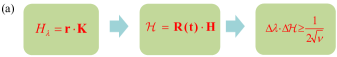
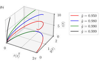
Figure 1: The image above is a flow diagram that includes a Hamiltonian $H_{\lambda}$ with the general form of su(1,1) Lie algebra, a Hermitian operator $\mathcal{H}$, and a parameter-dependent uncertainty relationship. Specifically, the analytic expression of the Hermitian operator $\mathcal{H}$ can be regarded as a brachistochrone problem on the $x-y$ plane and a monotone function of time in the $z$ direction (see Eqs. (3)-(5)). The image below provides a three-dimension graph and its projection on the $x-y$ plane for the Hermitian operator $\mathcal{H}$ in the isotropic quantum Rabi model (i.e., $\zeta=1$) with different effective coupling strengths $(\tilde{g}=0.950,0.980,0.990,0.999)$. Here the evolution time $t$ ranges from $0$ to $\pi/\omega\sqrt{1-\tilde{g}^{2}}$ with $\tilde{g}=0.950$.

Criticality in the quantum Rabi model.–Many studies have shown that there is a close relationship between quantum metrology and criticality, and the criticality may be a useful resource to enhance the accuracy of parameter evaluation. In this section, we analyze the relationship between quantum metrology and criticality from the perspective of Lie algebra structure. Quantum Rabi model (QRM) is a convenient model for parameter evaluation under different algebraic structures. The Hamiltonian of QRM reads ($\hbar=1$)

$$H_{\mathrm{Rabi}} =\omega a^{\dagger}a+\frac{\Omega}{2}\sigma_{z}+H_{c},$$ (11)

$$H_{\mathrm{c}} =g\left[(\sigma_{+}a+\sigma_{-}a^{\dagger})+\zeta(\sigma_{+}a^{\dagger}+\sigma_{-}a)\right].$$ (12)

Here, $a^{\dagger}(a)$ is the creation (annihilation) operator of the bose mode with frequency $\omega$; $\sigma_{k}(k=x,y,z)$ and $\sigma_{\pm}$ are the Pauli operators, the raising and lowering operators of the two-level system with transition frequency $\Omega$; $g$ and $\zeta$ represent the coupling strength and the ratio between rotating and counterrotating terms, respectively. When $\zeta=1$, this model is reduced to the isotropic QRM.

Using the Schrieffer-Wolff (SW) transformation on $H_{\mathrm{Rabi}}$ with a unitary operator $U_{\mathrm{sw}}=\exp\left\{-i(g/\Omega\sqrt{2})\left[(1-\zeta)\sigma_{x}p+(1+\zeta)\sigma_{y}x\right]\right\}$, and in the limit of $\Omega/\omega\rightarrow\infty$, an effective Hamiltonian in the spin-down subspace can be derived as [46, 48, 49],

$$H_{\mathrm{eff}}^{(\downarrow)}=\frac{\omega}{2}(1-g_{1}^{2})x^{2}+\frac{\omega}{2}(1-g_{2}^{2})p^{2},$$ (13)

where we have defined the dimensionless position and momentum operators $x=(a+a^{\dagger})/\sqrt{2}$ and $p=i(a^{\dagger}-a)/\sqrt{2}$. Here, $g_{1}=\tilde{g}(1+\zeta)/2$, $g_{2}=\tilde{g}(1-\zeta)/2$, with $\tilde{g}=2g/\sqrt{\Omega\omega}$ denoting the effective coupling strength. With the change of $\tilde{g}$, the QRM will undergo quantum phase transition at the point $\tilde{g}=\tilde{g}_{c}=2/(1+|\zeta|)$ [48], and we focus on the case of $\tilde{g}<\tilde{g}_{c}$ below. According to the one-mode bosonic realization of su(1,1) Lie algebra, the effective Hamiltonian Eq. (13) can be rewritten as [46]

$$H_{\mathrm{eff}}^{(\downarrow)}=2\omega K_{z}+\frac{\omega}{2}\lambda\left[K_{z}(1+\zeta^{2})+2\zeta K_{x}\right]\equiv H_{\lambda},$$ (14)

with the estimated parameter $\lambda=-\tilde{g}^{2}$. Based on the general form of Hamiltonian in Eq. (1), we can obtain $\boldsymbol{\mathrm{r}}$ and $|\boldsymbol{\mathrm{r}}|$. In fact, the value of $|\boldsymbol{\mathrm{r}}|$ is a pure imaginary number; for instance, $|\boldsymbol{\mathrm{r}}|=2\omega i\sqrt{1+\lambda}$ if $\zeta=1$. It can be seen from Eqs. (3)-(5) that the generator $\mathcal{H}$ in this model can be treated as an extended brachistochrone problem on the $x-y$ plane and the linear function of time in the $z$ direction. For the isotropic case of $\zeta=1$, the period of the cycloid equation becomes $\tau=\pi/\omega\sqrt{1+\lambda}$, which implies that the period will become infinite when the QRM operates in the phase transition point. As shown in Fig. 1(b), we plot a three-dimension graph and its projection on the $x-y$ plane for the generator $\mathcal{H}$ of the isotropic QRM with different effective coupling strengths $\tilde{g}$. We can vividly see that with the increase of the effective coupling strengths, the curve becomes shorter and shorter, which shows that we need more time to obtain an entire periodogram. In other words, the evolution time will tend to be infinite when the coupling strength is close to the phase transition point.

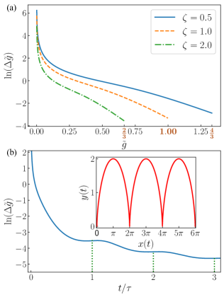
Figure 2: (a): Quantum Cramér-Rao bounds of the effective coupling strength $\tilde{g}$ are plotted as a function of $\tilde{g}$ with different rations $\zeta$, where the evolution time is fixed as $t=\pi/\omega$. (b): Quantum Cramér-Rao bound of the isotropic QRM ($\zeta=1$) is plotted as a function of the evolution time $t$ with a fixed coupling strength $\tilde{g}=0.9$ and the corresponding evolution period $\tau=\pi/\omega\sqrt{1-\tilde{g}^{2}}$. The inset describes the cycloid equation in the $x-y$ plane. The initial state of the system is a product state between the two subsystems, that is, the two-level system is in its spin-down state $|\!\downarrow\rangle$ and the bose field is $(|0\rangle+|1\rangle)/\sqrt{2}$.

With the expression of $\mathcal{H}$ in Eq. (2) and the Hamiltonian in Eq. (14), the analytical result of $\mathcal{H}$ in quantum Rabi model can be derived directly in this model. Then the QFI about the effective coupling strength $\tilde{g}$ can be obtained as

$$F_{\tilde{g}} =(\partial_{\tilde{g}}\lambda)^{2}F_{\lambda}=16\tilde{g}^{2}\Delta^{2}\mathcal{H}$$

$$=16\tilde{g}^{2}\boldsymbol{\mathrm{R(t)}}^{2}\Delta^{2}\boldsymbol{\mathrm{H}},$$ (15)

where $F_{\lambda}$ is the QFI about the estimated parameter $\lambda$, and the corresponding quantum Cramér-Rao bound is given by

$$\Delta\tilde{g}\geq 1/\sqrt{F_{\tilde{g}}}.$$ (16)

Through specific analytical derivation [46], we find that the uncertainty $\Delta\tilde{g}$ is actually a function that depends on the evolution time, the effective coupling strength $\tilde{g}$ and the ratio $\zeta$.

At first, we numerically simulate the relation between the uncertainty $\Delta\tilde{g}$ and the effective coupling strength $\tilde{g}$ for different $\zeta$, where the evolution time is fixed as $t=\pi/\omega$, as shown in Fig. 2(a). From the curves, we can see that for different $\zeta$, the value of the uncertainty $\Delta\tilde{g}$ decreases with the increase of $\tilde{g}$. Meanwhile, when the coupling strength $\tilde{g}$ is close to the phase transition point $\tilde{g}_{c}$ (i.e., $\frac{2}{3}$ for $\zeta=2.0$, $1$ for $\zeta=1.0$ and $\frac{4}{3}$ for $\zeta=0.5$), the uncertainty $\Delta\tilde{g}$ can obtain its minimum. Then, we analyze the relation of the uncertainty $\Delta\tilde{g}$ with the evolution time $t$ in the isotropic QRM ($\zeta=1$) for a given coupling strength $\tilde{g}=0.9$, as shown in Fig. 2(b). We can find that there is a close relation between the evolution of the uncertainty $\Delta\tilde{g}$ and the brachistochrone problem. Specifically, the value of $\Delta\tilde{g}$ periodically decreases with time $t$, and the period is consistent with the cycloid equation (see the inset of the figure). One can also analyze the case for a bigger coupling strength $\tilde{g}$. In this case, the period $\tau$ becomes longer and tends to be infinite when the coupling strength $\tilde{g}$ closes to the phase transition point $\tilde{g}_{c}$.

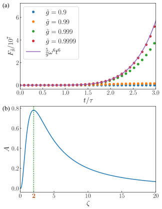
Figure 3: (a): QFIs $F_{\tilde{g}}$ of the isotropic QRM ($\zeta=1$) are plotted as a function the evolution time $t$ with different coupling strengths $\tilde{g}$ (i.e., $\tilde{g}=0.9,0.99,0.999,0.9999$). Here the value of the evolution period $\tau$ is consistent with that in Fig. 2. (b): Factor $A$ in the asymptotic expression of the QFI is plotted as a function of the ratio $\zeta$.

Above we have analyzed the evolution of the uncertainty $\Delta\tilde{g}$ with the coupling strength $\tilde{g}$ and the time $t$. Especially, we find that given a fixed coupling strength $\tilde{g}$, the evolution period of the uncertainty $\Delta\tilde{g}$ is consistent with the cycloid equation. Now, we investigate the properties of the system close to the phase transition point. With the result of the QFI $F_{\tilde{g}}$ in Eq. (15), we find that when the coupling strength $\tilde{g}$ tends to the phase transition point $\tilde{g}_{c}$, an asymptotic expression can be obtained as [46]

$$F_{\tilde{g}}\simeq A\omega^{6}t^{6},\quad\tilde{g}\rightarrow\tilde{g}_{c},$$ (17)

with the factor $A=320\zeta^{4}/9(1+\zeta)^{6}$. For the isotropic QRM, this asymptotic expression is reduced as $F_{\tilde{g}}\simeq 5\omega^{6}t^{6}/9$. We can find that when the coupling strength tends to its critical value, the QFI is proportional to the sixth power of the evolution time $t$. This implies that when approaching the phase transition point, the value of the QFI does not show divergent features, but is only a time-dependent function. Meanwhile, This time-dependent function is also related to the ratio $\zeta$. To better illustrate this feature, we numerically simulate the evolution of the QFI of the isotropic QRM with time, as shown in Fig. 3(a). From the curves, we can vividly see that when the coupling strength tends to the phase transition point, i.e, $\tilde{g}\rightarrow 1$, the QFI $F_{\tilde{g}}$ curve fits the asymptotic expression gradually. In addition, we also simulate the evolution of the factor $A$ in the asymptotic expression with the ratio $\zeta$, as shown in Fig. 3(b). We can see that there is a maximum for the factor $A$ when the ratio $\zeta=2$. This implies that for the anisotropic QRM with $\zeta=2$, the value of the QFI $F_{\tilde{g}}$ can obtain a maximum when the system tends to the phase transition point.

Conclusion–In summary, we investigate a unitary parametrization process governed by an su(1,1) Hamiltonian, and clarify the relationship between quantum metrology and criticality from the perspective of Lie algebra structure. We show that the generator $\mathcal{H}$ in the su(1,1) Hamiltonian can be treated as an extended brachistochrone problem on the $x-y$ plane and the linear function of time in the $z$ direction. In addition, we find that the uncertainty $\Delta\tilde{g}$ in the quantum Rabi model is actually a function that depends on the evolution time $t$, the effective coupling strength $\tilde{g}$ and the ratio $\zeta$. We also show that when the system tends to the phase transition point, the QFI $F_{\tilde{g}}$ is proportional to the sixth power of the evolution time, meanwhile, it can obtain a maximum when the ratio $\zeta=2$.