Active hypothesis testing in unknown environments using recurrent neural networks and model free reinforcement learning

Abstract

A combination of deep reinforcement learning and supervised learning is proposed for active sequential hypothesis testing in completely unknown environments. We make no assumptions about the prior probability, the action and observation sets, as well as the observation generating process. Experiments with synthetic Bernoulli and real cybersecurity data demonstrate that our method performs competitively and sometimes better than the Chernoff test, in both finite and infinite horizon problems.

I Introduction

In active sequential hypothesis testing (ASHT), a decision maker actively conducts a sequence of experiments in order to infer the underlying hypothesis from a finite set of hypotheses. The problem finds numerous applications including anomaly detection [1], medical diagnosis [2], radar assisted target search [3] and content search applications [4]. It has been extended to environments involving passive eavesdroppers [5] or active adversaries [6]. Deep reinforcement learning (DRL) techniques such as DQN [7] and deep actor critic algorithms were recently applied to ASHT (see [8], [9] and [6]). In these studies, the DRL agent selects actions based on beliefs over all possible hypotheses. Multiagent DRL methods for anomaly detection were proposed in [10] and [11].

In this work we consider belief free methods. The states of Deep recurrent neural networks (RNN)s are used as proxies for beliefs. We combine RNNs with reinforcement learning (RL) to address ASHT in environments with unknown observation probabilities and possibly infinite or continuous observations. At each time instance, the decision maker selects which experiment to conduct based on the history of past observations and actions. This is performed by a RNN network called RNNpolicy. Once the episode is terminated, the inference network, termed RNNinference is used to infer the hypothesis. In the infinite horizon setting, an additional RNN network, the so called RNNmonitor monitors the decision maker’s interaction with the environment and determines whether the experiments should terminate or continue. We assume that a training environment or a large dataset is available to train the networks. The actual environment in which the networks will be deployed can be slightly different, and the observation probabilities are unknown. Therefore, the agent can not take advantage of the belief vectors. In the case of anomaly detection over sensor networks [1], the size of the belief vector increases exponentially with the number of sensors. Consequently, quick decision making on large sensor networks by recursively updating beliefs and passing it through a large neural network to select the next query, may prove infeasible.

We apply a training procedure that includes the following steps. First we train the RNNpolicy on an artificial simulation environment using a DRL algorithm. A large dataset of actions and observations is created using the RNNpolicy network. Then the RNNmonitor is trained on data generated by the RNNpolicy using backpropagation [12]. Finally the pair RNNpolicy-RNNmonitor is used to create a second large dataset and the RNNinference is trained using backpropagation.

I-A Related work

In his seminal work [13], Chernoff proposed a heuristic called the Chernoff test and proved that it is asymptotically optimal under certain assumptions. In [14], a new variant of the test was introduced in the general multi-hypothesis testing. In [15] ASHT is modeled as a cost minimisation POMDP. The cost depends on the stopping time and the error probability. In [8], ASHT is modeled as a confidence maximisation belief MDP and a recurrent DQN [7] procedure is proposed and numerically shown to perform better than other heuristics. Similarly, in [9] a deep actor critic procedure is shown to perform better than the Chernoff test in environments that require high confidence levels.

I-B Our contribution

We propose a combination of DRL algorithms and RNNs to solve ASHT problems in completely unknown environments. We make no assumptions about the prior probability of the hypotheses, the observation generating process or the type of observations. In fact continuous action spaces are allowed. The only requirement is access to a training environment, or an appropriate training dataset. We compare our approach to the modified Chernoff test of [14] in environments with discrete, finite actions and observations, and show that the proposed method achieves competitive results and sometimes performs slightly better.

The rest of this paper is organised as follows. ASHT is defined in section II. The proposed method is presented in section III for finite and infinite horizons. Comparisons with the Chernoff test are given in sections IV and V using anomaly detection environments. Further information about the experiments and sample efficiency analysis is presented as appendix in the extended version.

II Problem statement

Let $\mathcal{X}=\{0,1,...,N\}$ be a finite set of hypotheses. The random variable $X$ defines the true hypothesis. At each time $t>0$ a decision maker chooses an action $a_{t}\in\mathcal{A}$. Based on $a_{t}$ and $X=x$, an observation $y_{t}\in\mathcal{Y}$ is generated. Typically it is assumed that these observations are i.i.d, sampled from a known distribution $p_{X}^{a_{t}}\triangleq P[Y|X,a_{t}],$ while both actions and observations belong to finite sets. None of these assumptions are required in this work. Actions aim to assist inference of the true hypothesis. They rely on the information available at time $t$: $I_{t}=\{a_{1:t-1},y_{1:t-1}\},$ and are sampled from a belief based policy. For a given action $a_{t}$ and observation $y_{t}$, the belief on each hypothesis $i\in\mathcal{X}$ is updated recursively as

$$\rho_{t+1}(i)=\rho_{t}(i)\frac{p_{i}^{a_{t}}(y_{t})}{\sum_{j}\rho_{t}(j)p_{j}^{a_{t}}(y_{t})}.$$ (1)

$\rho_{0}$ is the prior probability that a hypothesis is true.

The inferred hypothesis is denoted by $\hat{X}_{t}$ and is the result of the inference policy acting on the information set.

The quality of inference is measured by several indicators. The error probability is expressed in terms of beliefs as $\gamma_{t}=P[\hat{X}_{t}\neq X]=1-\max_{i}\rho_{t}(i).$ The average confidence level is given by

$$C(\rho)=\sum_{i\in\mathcal{X}}\rho(i)\log\bigg{(}\frac{\rho(i)}{1-\rho(i)}\bigg{)}.$$ (2)

The following index

$$LL_{t}=log\frac{p_{\hat{i}_{t}}(y_{1:t},a_{1:t})}{\max_{j\neq\hat{i}_{t}}p_{j}(y_{1:t},a_{1:t})},$$ (3)

where $\hat{i}_{t}$ is the most likely hypothesis monitors performance in the infinite horizon setting. It provides an asymptotically optimal stopping rule: the agent terminates the experiment the first time $t$ for which $LL_{t}>-\log c,$ where $c$ is a positive real valued parameter. Upon termination, the inference strategy selects the hypothesis $\hat{i}_{t}$ that maximizes the aposteriori probability (MAP decoding) or the likelihood (ML decoding). Often a uniform prior is employed, in which case the MAP and ML decoding rules coincide. For further details please see [8] and [6].

An asympotically optimal policy is given by the Chernoff test. At each time $t$, actions are sampled from the distribution

$$g_{t}=\max_{g}\min_{j\neq\hat{i}_{t}}\sum_{a}g(a)D(p_{\hat{i}}^{a}||p_{j}^{a}).$$ (4)

III Architecture and training procedure

Figure 1: Architecture. RNNmonitor decides whether to continue based on the information set. Then either RNNinference guesses the underlying hypothesis or RNNpolicy continues with experiment selection.

In this section, we combine DRL and supervised learning to tackle ASHT without the use of belief vectors. We assume that we have access to a training environment or alternatively, to a large dataset, based on which we can build a simulator. A schematic plot of the proposed architecture is given in fig 1.

Two supervised neural networks are in charge of termination time and inference, and one (or two for actor critic algorithms) is in charge of experiment selection. We employ recurrent neural networks (RNN) rather than feedforward neural networks to take advantage of their capacity to model dynamic input output systems. Simple RNNs are prone to numerical instability problems, most notably vanishing and exploding gradients. To remedy these issues, several variations have been proposed, most notably, long short term memory networks (LSTM)s [16] and Gated recurrent units (GRU)s [17], which have been successfully applied to POMDP agents, [18] and [19]. In this work we consider both LSTM and GRU networks.

Under the infinite horizon setting we employ two recurrent neural networks for decoding, RNNmonitor and RNNinference. The first network monitors the environment at each time instance. The value determined by its output is used to decide whether the process continues or terminates on the basis of a threshold rule. The second network is activated when the RNNmonitor decides termination. It produces an estimate of the underlying true hypothesis. Under the fixed finite horizon case, the RNNmonitor becomes redundant. The structure of the two recurrent networks is identical except from the final layer which performs the regression and classificatin tasks respectively.

Each network is fed by the sequence of action and observation pairs. At each time $t$, a tuple $(a_{t},y_{t})$ passes through the RNN cell and an output $o_{t}$ is generated. The mean of all outputs goes through a feed forward layer that outputs the prediction. In the case of classification, the feed forward layer is followed by a softmax activation function. The loss function of RNNinference is the cross entropy loss between the true hypothesis $X$ and the predicted hypothesis. The loss function of RNNmonitor is the mean squared error loss. All networks are developed using the pytorch framework [20]. A high level overview of RNNinference is provided at fig 2.

Figure 2: A high level overview of RNNInference. Each action observation pair $(a_{t},y_{t})$ passes through a RNN architecture and outputs $o_{t}$. All outputs are averaged and passed through a feed forward layer. Finally a softmax activation function produces an estimate of the true hypothesis. A similar architecture is employed by RNNMonitor, without the softmax function.

Training of the neural networks takes place in three phases. First, we train the RNNpolicy network using reinforcement learning on an artificial simulation environment. Then the RNNmonitor and subsequently the RNNinference are trained using the adam optimizer [21]. In the fixed horizon setting, training of the RNNmonitor is deactivated.

The RNNpolicy is initialised with random parameters. The artificial simulation environment is created as follows. At each training episode the underlying hypothesis $i$ is sampled from $\mathcal{X}$ according to $\rho_{0}$. At each time $t$ the agent chooses an action $a_{t}$ based on the state of the recurrent neural network and its most recent observation $y_{t-1}$ (action $a_{1}$ is chosen randomly). An observation $y_{t}$ is sampled from $\mathcal{Y}$ according to $P[Y|X=i,a=a_{t}]$. The training environment internally updates the belief vector $\rho_{t}$. The reward provided to the agent is the error improvement $\gamma_{t-1}-\gamma_{t}$. After $T$ time steps the training episode terminates. In the finite horizon setting, $T$ defines the horizon length. In the infinite horizon setting, we set $T$ to a large value to ensure sufficient exploration. We use a reliable open source implementation of recurrent PPO [22] (contributed version).

Upon completion of phase 1 and training of the RNNpolicy network, a new dataset is generated by randomly selecting the horizon of each episode. Each data point consists of a sequence of actions and observations labeled by the error probability at the final time step. The resulting dataset is used to train RNNmonitor in stage 2.

Finally training of RNNinference is realized via a new dataset generated as follows. At each time instance $t$ of each training episode, RNNmonitor outputs an approximation of the error probability $\bar{\gamma}_{t}$. If $\bar{\gamma}_{t}<c$, where the hyperparameter $c$ is a user defined threshold, the episode terminates, else RNNpolicy continues with the experiment selection. The label of each data point is the underlying true hypothesis. The desired dataset is obtained by repeating this procedure for multiple episodes.

In the execution phase, the three networks are run and evaluated in a testing environment which slightly differs from the one they are trained on.

IV Case study: Anomaly detection

We consider an anomaly detection example involving two sensors $\mathcal{A}$ and $\mathcal{B}$ that detect anomalies in their proximity. There are 4 possible hypotheses. $X=0$ means there is no anomaly (the system is in safe state). $X=1$ and $X=2$ mean there is an anomaly near sensors $\mathcal{A}$ and $\mathcal{B}$ respectively. Finally, $X=3$ means there are anomalies near both sensors. We assume a uniform prior. We create two slightly different environments, one for training the DRL agent and the RNN decoders and one for testing their performance. The observation models are summarized in tables I and II.

TABLE I: $P[Y=1|a_{t},X]$ under training

	$X=0$	$X=1$	$X=2$	$X=3$
$\mathcal{A}$	0.2	0.8	0.2	0.8
$\mathcal{B}$	0.2	0.2	0.8	0.8

TABLE II: $P[Y=1|a_{t},X]$ under testing

	$X=0$	$X=1$	$X=2$	$X=3$
$\mathcal{A}$	0.25	0.75	0.25	0.75
$\mathcal{B}$	0.15	0.15	0.85	0.85

First we examine how efficiently LSTMs and GRUs learn to map action and observation sequences to $\gamma_{t}$, $LL_{t}$, $C_{t}$ and $\hat{i}_{t}$, where $\hat{i}_{t}$ is the most likely hypothesis. We follow the modified Chernoff strategy in the training environment as described in [14], and collect a dataset of 60000 sequences. The first 50000 are used for training and the rest for validation. We also build a test set of 10000 sequences using the testing environments. We pick a fixed horizon at the beginning of each episode, randomly in the range 5-50.

We consider unidirectional and bidirectional RNNs with two hidden layers and size in the range 50-400. The RNN with the best score on the validation set is used in the test set. In case of ties, the simpler architecture is preferred. The results for all 5 metrics are shown in table III.

We note that as the error probability becomes small, both $LL_{t}$ and $C_{t}$ can be large. Moreover, they might take small or even negative values for small horizons. Hence we discarded all samples where $LL_{t}>100$, because the maximum absolute error (MAE) was very large. On the other hand $\gamma_{t}$ is always in the range $[0,1]$. It can be seen from table III that both LSTMs and GRUs learn $\hat{j}_{t}$ and $\gamma_{t}$ very accurately. For this reason, the stopping rule in the infinite horizon setting employs the error probability.

TABLE III: Test scores and size parameters.

	LSTM	GRU
best hidden size for $LL_{t}$	400(BI)	300 (BI)
best hidden size for $\hat{j}_{t}$	200	200
best hidden size for $C(\rho_{t})$	250(BI)	250(BI)
best hidden size for $\gamma_{t}$	200	250
precision on $\hat{j}_{t}$	0.9996	0.9967
recall on $\hat{j}_{t}$	0.9996	0.996
f1 score on $\hat{j}_{t}$	0.9996	0.9996
MAE for $LL_{t}$	13.25	14.397
MAE for $C(\rho_{t})$	0.952	0.945
MAE for $\gamma_{t}$	0.00085	0.0019

We explore different horizons of length 10, 25, 50, and 100. For each horizon, the PPO agent is trained and a dataset that has 60000 different sequences of actions and observations is generated. Both decoders are unidirectional RNNs with 2 hidden layers of the same size. The GRU decoder has 250 hidden units and the LSTM decoder 200 units. When paired with a GRU or an LSTM decoder, for horizons 10-50, PPO’s performance is comparable to that of the Chernoff test . In fact, for $T=10$ it achieves a smaller error probability. For $T=100$, the Chernoff test achieves a significantly smaller error probability. The GRU decoder performs slightly better than the LSTM decoder.

TABLE IV: Average error probability over 10000 episodes

T	PPO-LSTM	PPO-GRU	Chernoff
10	0.152	0.151	0.162
25	0.0396	0.0341	0.0312
50	0.0078	0.008	0.0017
100	0.0008	0.0007	0.00005

In the infinite horizon case, we use the PPO agent previously trained for $T=50$. The dataset consists of 60000 training examples. The horizon of each episode is chosen uniformly in the range [1,50]. The LSTM network approximates the error probability. When the network detects that the error probability is below a user defined threshold $c$, the episode terminates. Using the agent and the network a new dataset of 60000 examples is generated and used to train another LSTM that infers the underlying hypothesis. We tested the PPO agent based on the LSTM networks in the test environments for 10000 episodes. We repeated the procedure for GRU networks. The test results for different tolerance levels are demonstrated in table V.

The LSTM networks are bidirectional with 2 hidden layers of 200 neurons. They also employ dropout with probability $p=0.2$. The GRUs are bidirectional with 4 hidden layers of 250 neurons. Again, dropout is used with $p=0.2$.

Contrary to the finite horizon, LSTM decoders perform better than GRU decoders. When the PPO agent is combined with LSTM decoders, it terminates at the desired error probability level slightly faster than the Chernoff test in 2/4 experiments.

TABLE V: Average stopping time and error probability

(a) stopping time

c	PPO-LSTM	PPO-GRU	Chernoff
0.3	5.85	6	4.58
0.2	7.41	8	7.73
0.1	11.58	13	12.61
0.05	12.66	16.14	12.164

(b) error probability

c	PPO-LSTM	PPO-GRU	Chernoff
0.3	0.198	0.205	0.248
0.2	0.134	0.164	0.131
0.1	0.075	0.092	0.046
0.05	0.043	0.051	0.038

V Further examples

Next we consider a larger anomaly detection problem. Four sensors monitor four independent random processes. Any number of processes can be abnormal, therefore there are 16 different hypotheses. Proceeding as in the previous chapter, we build two slightly different training and testing environments. When a process is abnormal in the training environment the sensor outputs 1 with probability 0.8 and 0 with probability 0.2. When the process is normal the numbers are reversed. In the testing environment, the first two sensors output 1 with probability 0.85 when the processes are abnormal, and the last two output 1 with probability 0.75.

We repeat the fixed horizon experiments, only this time, the training dataset consists of 150000 examples. The network pairs are tested for 10000 episodes. The results for different horizons are summarized in table VI.

TABLE VI: Average error probability in the four sensors case

horizons	PPO+LSTM	PPO+GRU	Chernoff
10	0.48	0.49	0.53
25	0.247	0.245	0.234
50	0.0698	0.0699	0.071
100	0.0238	0.0157	0.008

Both network pairs perform better than the Chernoff test for horizons of length 10 and 50. For horizons 25 and 100, the Chernoff test performs slightly better.

Next we consider an anomaly detection example that lies closer to real world data, namely the windows 10 dataset from the TON_IOT cybersecurity data [23]. More information about how the environment works is provided in the extended version of this paper available at arxiv.

We repeat the experiments of table VI. The results are shown in table VII. Our method performs better than the Chernoff test for horizons $T=10$ and $T=25$, and the difference for $T=50$ and $T=100$ is very small (one error out of 10000 episodes).

TABLE VII: Average error probability out of 10000 episodes for the cybersecurity data.

horizons	PPO+LSTM	PPO+GRU	Chernoff
10	0.0632	0.0634	0.2314
25	0.0064	0.0057	0.0194
50	0001	0.0002	0.0001
100	0.001	0	0

The sample efficiency of the supervised decoders and the recurrent PPO algorithm are analyzed in the extended version. The DRL algorithm requires far more samples than the supervised decoders.

VI Conclusion

We have demonstrated that model free recurrent DRL combined with RNN decoders can successfully be applied to ASHT environments. Unlike other approaches, our method does not need to recursively construct large belief or likelihood vectors, hence it can scale up to very large environments. We have also employed different training and testing environments. The proposed method performs competitively with the asymptotically optimal Chernoff test, both in finite and infinite horizon problems, despite the lack of knowledge of the observation probabilities. For smaller horizons it usually performs better.

In future work we will seek to improve the sample complexity of the DRL part of our method, and apply offline (batch) reinforcement learning for large environments when there is not an accurate simulator and only a fixed dataset. We will consider replacing LSTMs and GRUs with transformers [24].

VII Extended version: Testing and Training on cybersecurity data

Each entry of the dataset contains information about one process running in a windows 10 PC. It provides information on the processes characteristics such as the activity of processor, network, memory and disk. Each process has a binary label about its status (normal or abnormal). we ignore the second label describing the type of attack. The following five features are chosen:

1. ’Memory Demand Zero Faults sec’ ,

2. ’Network_I(Intel R _82574L_GNC)Bytes Received sec’,

3. ’Network_I(Intel R _82574L_GNC) Bytes Sent sec’,

4. ’Process_Page Faults_sec’,

5. ’Memory Page Writes sec’,

we used the default sklearn implementation of a decision tree [25], setting class_weight=’balanced’, combined with a standard scaler, to perform classification.

We split the windows 10 dataset in three sets a training set, a validation set, and a test set. The model is trained on the training set, and the conditional observation probabilities are estimated on the validation set. They are then used to train the algorithm.

The testing environment works as follows. First, the true hypothesis is sampled from the uniform prior. Then, at each time, depending on whether the queried process is normal or not we sample an entry from the test set and pass it from the trained decision tree classifier. The output of the classifier ($0$ or $1$) is used to update the belief. The other features of the environment remain unchanged.

VII-A Sample efficiency

We set $T=25$ and collect datasets of different sizes from $100$ to $150000$ to train the decoders using an already trained PPO-LSTM agent. The testing remains the same. The error probabilities are illustrated in Figures 3 and 4 respectively. We observe that after $1000$ training examples the error probability becomes very small, and after $20000$ it is near zero and does not decrease significantly any further. Results for other horizons are similar.

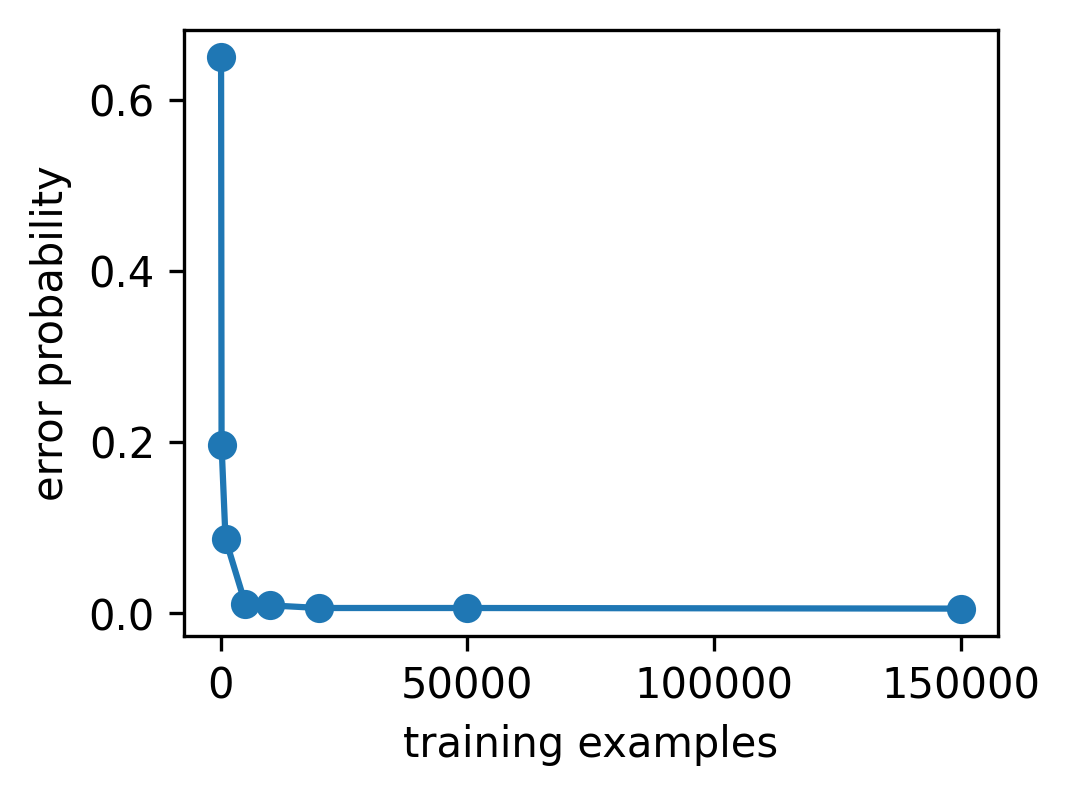
Figure 3: Error probability of the GRU decoder for different dataset sizes

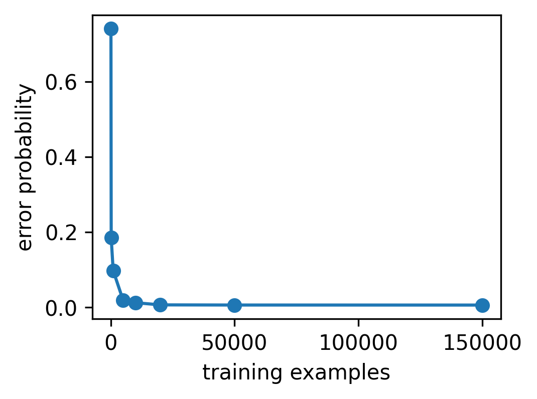
Figure 4: Error probability of the LSTM decoder for different dataset sizes

Next, we evaluate the sample efficiency of the PPO-LSTM algorithm. We trained the model for a large number of episodes and interrupted for testing every $5000$ episodes. For testing we use the MAP decoder. The results are shown in figure 5.

We observe that the algorithm is more sample efficient for smaller horizons and the decoders need far fewer samples than the DRL algorithm.

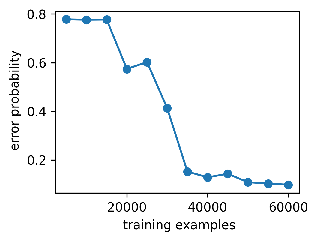
(a) T=10

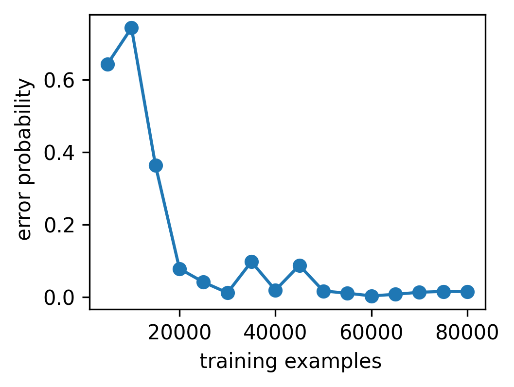
(b) T=25

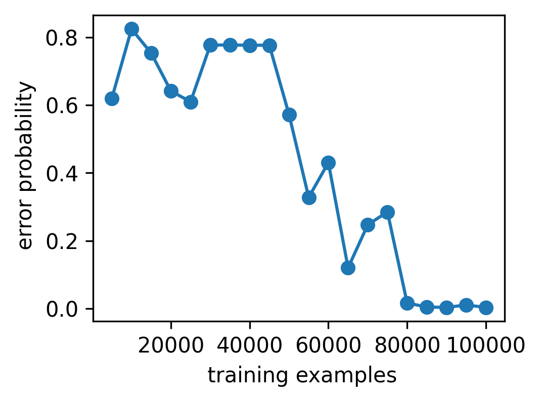
(c) T=50

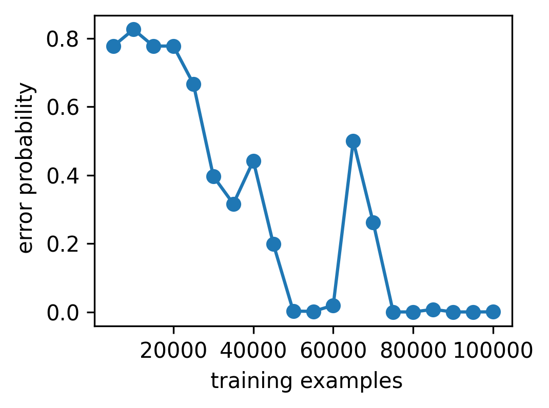
(d) T=100

Figure 5: Sample efficiency of PPO-LSTM for different horizons

References

- [1] K. Cohen and Q. Zhao, “Active hypothesis testing for anomaly detection,” IEEE Transactions on Information Theory, vol. 61, no. 3, pp. 1432–1450, 2015.
- [2] S. M. Berry, B. P. Carlin, J.-K. J. Lee, and P. Müller, “Bayesian adaptive methods for clinical trials,” 2010.
- [3] M. Franceschetti, S. Marano, and V. Matta, “Chernoff test for strong-or-weak radar models,” IEEE Transactions on Signal Processing, vol. 65, no. 2, pp. 289–302, 2017.
- [4] F. Cecchi and N. Hegde, “Adaptive active hypothesis testing under limited information,” in Advances in Neural Information Processing Systems (I. Guyon, U. V. Luxburg, S. Bengio, H. Wallach, R. Fergus, S. Vishwanathan, and R. Garnett, eds.), vol. 30, Curran Associates, Inc., 2017.
- [5] M.-C. Chang and M. R. Bloch, “Evasive active hypothesis testing,” IEEE Journal on Selected Areas in Information Theory, vol. 2, no. 2, pp. 735–746, 2021.
- [6] N. Kalouptsidis and G. Stamatelis, “Deep reinforcement learning and adaptive strategies for adversarial active hypothesis testing,” under review, 2022.
- [7] V. Mnih, K. Kavukcuoglu, D. Silver, A. A. Rusu, J. Veness, M. G. Bellemare, A. Graves, M. Riedmiller, A. K. Fidjeland, G. Ostrovski, S. Petersen, C. Beattie, A. Sadik, I. Antonoglou, H. King, D. Kumaran, D. Wierstra, S. Legg, and D. Hassabis, “Human-level control through deep reinforcement learning,” Nature, vol. 518, pp. 529–533, Feb. 2015.
- [8] D. Kartik, E. Sabir, U. Mitra, and P. Natarajan, “Policy design for active sequential hypothesis testing using deep learning,” in 2018 56th Annual Allerton Conference on Communication, Control, and Computing (Allerton), pp. 741–748, 2018.
- [9] C. Zhong, M. C. Gursoy, and S. Velipasalar, “Deep actor-critic reinforcement learning for anomaly detection,” in 2019 IEEE Global Communications Conference (GLOBECOM), pp. 1–6, 2019.
- [10] H. Szostak and K. Cohen, “Decentralized anomaly detection via deep multi-agent reinforcement learning,” in 2022 58th Annual Allerton Conference on Communication, Control, and Computing (Allerton), pp. 1–4, 2022.
- [11] G. Joseph, C. Zhong, M. C. Gursoy, S. Velipasalar, and P. K. Varshney, “Scalable and decentralized algorithms for anomaly detection via learning-based controlled sensing,” 2021.
- [12] D. E. Rumelhart, G. E. Hinton, and R. J. Williams, “Learning representations by back-propagating errors,” Nature, vol. 323, pp. 533–536, 1986.
- [13] H. Chernoff, “Sequential design of experiments,” The Annals of Mathematical Statistics, vol. 30, no. 3, pp. 755–770, 1959.
- [14] S. Nitinawarat, G. K. Atia, and V. V. Veeravalli, “Controlled sensing for multihypothesis testing,” IEEE Transactions on Automatic Control, vol. 58, no. 10, pp. 2451–2464, 2013.
- [15] M. Naghshvar and T. Javidi, “Active sequential hypothesis testing,” The Annals of Statistics, vol. 41, dec 2013.
- [16] S. Hochreiter and J. Schmidhuber, “Long short-term memory,” Neural Computation, vol. 9, no. 8, pp. 1735–1780, 1997.
- [17] J. Chung, C. Gulcehre, K. Cho, and Y. Bengio, “Gated feedback recurrent neural networks,” in Proceedings of the 32nd International Conference on Machine Learning (F. Bach and D. Blei, eds.), vol. 37 of Proceedings of Machine Learning Research, (Lille, France), pp. 2067–2075, PMLR, 07–09 Jul 2015.
- [18] M. Hausknecht and P. Stone, “Deep recurrent q-learning for partially observable mdps,” in AAAI Fall Symposium on Sequential Decision Making for Intelligent Agents (AAAI-SDMIA15), November 2015.
- [19] T. Ni, B. Eysenbach, and R. Salakhutdinov, “Recurrent model-free rl can be a strong baseline for many pomdps,” 2021, Available at: Arxiv:2110.05038.
- [20] A. Paszke, S. Gross, F. Massa, A. Lerer, J. Bradbury, G. Chanan, T. Killeen, Z. Lin, N. Gimelshein, L. Antiga, A. Desmaison, A. Kopf, E. Yang, Z. DeVito, M. Raison, A. Tejani, S. Chilamkurthy, B. Steiner, L. Fang, J. Bai, and S. Chintala, “Pytorch: An imperative style, high-performance deep learning library,” in Advances in Neural Information Processing Systems (H. Wallach, H. Larochelle, A. Beygelzimer, F. d'Alché-Buc, E. Fox, and R. Garnett, eds.), vol. 32, Curran Associates, Inc., 2019.
- [21] D. Kingma and J. Ba, “Adam: A method for stochastic optimization,” International Conference on Learning Representations, 12 2014.
- [22] A. Raffin, A. Hill, M. Ernestus, A. Gleave, A. Kanervisto, and N. Dormann, “Stable baselines3.” https://github.com/DLR-RM/stable-baselines3, 2019.
- [23] N. Moustafa, M. Keshk, E. Debie, and H. Janicke, “Federated ton_iot windows datasets for evaluating ai-based security applications,” 2020.
- [24] A. Vaswani, N. Shazeer, N. Parmar, J. Uszkoreit, L. Jones, A. N. Gomez, L. u. Kaiser, and I. Polosukhin, “Attention is all you need,” in Advances in Neural Information Processing Systems (I. Guyon, U. V. Luxburg, S. Bengio, H. Wallach, R. Fergus, S. Vishwanathan, and R. Garnett, eds.), vol. 30, Curran Associates, Inc., 2017.
- [25] F. Pedregosa, G. Varoquaux, A. Gramfort, V. Michel, B. Thirion, O. Grisel, M. Blondel, P. Prettenhofer, R. Weiss, V. Dubourg, J. Vanderplas, A. Passos, D. Cournapeau, M. Brucher, M. Perrot, and E. Duchesnay, “Scikit-learn: Machine learning in Python,” Journal of Machine Learning Research, vol. 12, pp. 2825–2830, 2011.