Entangled state dynamics of moving two-level atoms in a thermal field bath

Abstract

We consider a two-level atom that follows a wordline of constant velocity, while interacting with a massless scalar field in a thermal state through: (i) an Unruh-DeWitt coupling, and (ii) a coupling that involves the time derivative of the field. We treat the atom as an open quantum system, with the field playing the role of the environment, and employ a master equation to describe its time evolution. We study the dynamics of entanglement between the moving atom and a (auxiliary) qubit at rest and isolated from the thermal field. We find that in the case of the standard Unruh-DeWitt coupling and for high temperatures of the environment the decay of entanglement is delayed due to the atom's motion. Instead, in the derivative coupling case, the atom's motion always causes the rapid death of entanglement.

I Introduction

Quantum entanglement [1], which describes the non-local correlations between different quantum systems, is considered one of the most striking features of quantum theory. The past few years, entanglement has been recognised as a valuable resource for quantum information processing. It lies at the heart of many applications, such as teleportation [2, 3], cryptography [4, 5], and communication through dense coding [6], while it is necessary for the exponential speed–up of quantum computations over classical ones [7, 8].

However, in realistic conditions, the inevitable interaction of quantum systems with their surrounding environments results in a rapid loss, and an eventual death of entanglement at finite times (see, e.g., [9] and references therein). This fragility of entanglement has become one of the main issues in the realization of practical quantum technologies. To protect entangled states from the decoherence induced by the system-environment interactions, various techniques have been developed in the past, including dynamical decoupling [10], the use of the quantum Zeno effect [11, 12] and decoherence-free subspaces [13].

In the present article, motivated by the works [14, 15], we study the dynamics of entanglement between two two-level atoms, with the one moving at a constant velocity through a massless scalar field in a thermal state and the other at rest and isolated from the field. We employ two different models to describe the atom-field interaction: (i) the standard Unruh-DeWitt (UDW) particle detector model [16, 17, 18, 19], which linearly couples the atom with the field, and (ii) a derivative coupling model that couples the atom with the time derivative of the field [20, 21, 22, 23, 24]. We find that in the first case, the motion of the atom can slow the rate at which entanglement is lost due to its interaction with a high temperature environment. This suggests the use of an atom's (relativistic) motion as a method to counter entanglement loss in quantum systems. On the other hand, in the derivative coupling case, we observe that an increase in the atom’s velocity causes a rapid degradation of entanglement.

II Two-level atom moving through a thermal field bath

We begin our analysis by introducing the UDW detector model. We then treat a detector that is moving with constant velocity as an open quantum system, with a scalar field in a thermal state playing the role of the environment. We employ a Markovian master equation to describe its time evolution.

Throughout the paper we denote spatial vectors with boldface letters $(\mathbf{x})$, while spacetime vectors are represented by sans-serif characters $(\mathsf{x})$. We use the signature $(-+++)$ for the Minkowski spacetime metric. Unless otherwise specified we hereafter set $\hbar=c=k_{B}=1$.

II.1 The Unruh-DeWitt detector model

We consider a massless scalar quantum field $\hat{\phi}(\mathsf{x})$ in the (3+1)-dimensional Minkowski spacetime with metric $\eta_{\mu\nu}$. The scalar field satisfies the Klein-Gordon equation $\square\hat{\phi}(\mathsf{x})=0$, where $\square=\eta^{\mu\nu}\partial_{\mu}\partial_{\nu}=-\partial_{t}^{2}+\nabla^{2}$ is the d'Alembert operator. In terms of plane wave solutions to the Klein-Gordon equation the field can be expressed as

$$\hat{\phi}(\mathsf{x})=\int\frac{d^{3}\boldsymbol{k}}{\sqrt{(2\pi)^{3}2|\boldsymbol{k}|}}\left(\hat{a}_{\boldsymbol{k}}e^{-i(|\boldsymbol{k}|t-i\boldsymbol{k}\cdot\mathbf{x})}+\text{H.c.}\right),$$ (1)

where $\hat{a}_{\boldsymbol{k}}$ and $\hat{a}_{\boldsymbol{k}}^{\dagger}$ are the annihilation and creation operators of the field mode with momentum $\boldsymbol{k}$. They satisfy the canonical commutation relations

$$[\hat{a}_{\boldsymbol{k}},\hat{a}_{\boldsymbol{k}^{\prime}}^{\dagger}]=\delta^{3}(\boldsymbol{k}-\boldsymbol{k}^{\prime}),\quad[\hat{a}_{\boldsymbol{k}},\hat{a}_{\boldsymbol{k}^{\prime}}]=[\hat{a}_{\boldsymbol{k}}^{\dagger},\hat{a}_{\boldsymbol{k}^{\prime}}^{\dagger}]=0.$$ (2)

The free Hamiltonian of the field, after subtracting the infinite zero-point energy, reads

$$\hat{H}_{\phi}=\int d^{3}\boldsymbol{k}|\boldsymbol{k}|\hat{a}_{\boldsymbol{k}}^{\dagger}\hat{a}_{\boldsymbol{k}}.$$ (3)

We consider an Unruh-DeWitt (UDW) particle detector [16, 17, 18, 19] modeled as a pointlike two-level atom with energy gap $\omega$ and Hamiltonian

$$\hat{H}_{0}=\frac{\omega}{2}\hat{\sigma}_{3},$$ (4)

where $\hat{\sigma}_{3}$ is the usual Pauli operator. The detector moves along a worldline $\mathsf{x}(\tau)=(t(\tau),\mathbf{x}(\tau))$ parametrized by its proper time $\tau$, while interacting with the scalar field through the interaction Hamiltonian

$$\hat{H}_{\text{int}}(\tau)=\lambda(\tau)\hat{\mu}(\tau)\otimes\frac{d^{p}}{d\tau^{p}}\hat{\phi}(\tau),$$ (5)

where $\lambda(\tau)$ describes how the coupling between the detector and the field is switched on and off,

$$\hat{\mu}(\tau)=e^{i\omega\tau}\hat{\sigma}_{+}+e^{-i\omega\tau}\hat{\sigma}_{-}$$ (6)

is the detector's monopole moment operator expressed in terms of the SU(2) ladder operators $\hat{\sigma}_{\pm}$, $\hat{\phi}(\tau):=\hat{\phi}(\mathsf{x}(\tau))$ is the scalar field operator evaluated along the detector's trajectory, and $p$ is a non-negative integer. We will next consider a sudden switching $\lambda(\tau)=\lambda\theta(\tau)$, where $\lambda$ specifies the detector-field coupling strength and $\theta(\tau)$ is the Heaviside step function.

In this work, we will focus on the cases: (i) $p=0$, which refers to the standard UDW detector model, and (ii) $p=1$, which corresponds to a derivative coupling detector model [20, 21, 22, 23, 24] that linearly couples the atom with the proper-time derivative of the quantum field. The derivative coupling model closely resembles the dipole interaction $\hat{\mathbf{d}}\cdot\hat{\mathbf{E}}$ between an atom with dipole moment $\hat{\mathbf{d}}$ and an external electromagnetic field $\hat{\mathbf{E}}(t,\boldsymbol{x})=-\partial_{t}\hat{\mathbf{A}}(t,\boldsymbol{x})$ expressed in terms of the vector potential $\hat{\mathbf{A}}$ (in the Coulomb gauge)[25].

In the followings, we will consider that the detector is moving with a constant velocity $\upsilon$ along the trajectory [18]

$$\mathsf{x}(\tau)=(\gamma\tau,\gamma\upsilon\tau,0,0),$$ (7)

where $\gamma=1/\sqrt{1-\upsilon^{2}}$ is the Lorentz factor.

II.2 The Markovian master equation

We treat the detector as an open quantum system [26], with the scalar field playing the role of the environment. We suppose that initially the field is in a thermal state

$$\hat{\rho}_{\beta}=\frac{e^{-\beta\hat{H}_{\phi}}}{\text{tr}(e^{-\beta\hat{H}_{\phi}})}$$ (8)

at temperature $T=\beta^{-1}$, and that no correlations between the detector and the field environment are present, i.e., $\hat{\rho}_{\text{tot}}(0)=\hat{\rho}(0)\otimes\hat{\rho}_{\beta}$.

The dynamics of the density operator of the combined detector-field system in the interaction picture is described by the Liouville-von Neumann equation

$$\frac{d}{d\tau}\hat{\rho}_{\text{tot}}(\tau)=-i[\hat{H}_{\text{int}}(\tau),\hat{\rho}_{\text{tot}}(\tau)],$$ (9)

where $[\cdot,\cdot]$ stands for the commutator. We can formally solve Eq. (9) by integration to obtain

$$\hat{\rho}_{\text{tot}}(\tau) =\hat{\rho}_{\text{tot}}(0)-i\int_{0}^{\tau}ds[\hat{H}_{\text{int}}(s),\hat{\rho}_{\text{tot}}(s)].$$ (10)

Inserting then the integral form (10) back into (9) and taking the partial trace over the field bath degrees of freedom yields an integro-differential equation for the reduced density matrix of the detector

$$\dot{\hat{\rho}}(\tau)=-\int_{0}^{\tau}ds\,\text{tr}_{\phi}[\hat{H}_{\text{int}}(\tau),[\hat{H}_{\text{int}}(s),\hat{\rho}_{\text{tot}}(s)]].$$ (11)

We next successively employ: (i) the Born approximation, that is we assume a weak coupling between the detector and the field so that the combined state $\hat{\rho}_{\text{tot}}(s)\simeq\hat{\rho}(s)\otimes\hat{\rho}_{\beta}$ remains approximately factorized at all times, and (ii) the Markov approximation, by which we replace $\hat{\rho}(s)$ by $\hat{\rho}(\tau)$ in the integral in (11) and extend the upper limit of integration to infinity. The Markov approximation is valid provided that the detector's time evolution is much slower than that of the field bath [27]. After performing a change of variables $s\to\tau-s$ we obtain the Markovian master equation

$$\dot{\hat{\rho}}(\tau)=-\int_{0}^{\infty}ds\,\text{tr}_{\phi}[\hat{H}_{\text{int}}(\tau),[\hat{H}_{\text{int}}(\tau-s),\hat{\rho}(\tau)\otimes\hat{\rho}_{\beta}]].$$ (12)

In terms of the interaction Hamiltonian (5) the above master equation takes the form [28, 29]

$$\dot{\hat{\rho}}(\tau)=-\int_{0}^{\infty}ds\Big{(}[\hat{\mu}(\tau),\hat{\mu}(\tau-s)\hat{\rho}(\tau)]\mathcal{W}(\tau,\tau-s)+\text{H.c.}\Big{)},$$ (13)

where

$$\mathcal{W}(\tau,\tau^{\prime}):=\text{tr}_{\phi}\Big{(}\hat{\rho}_{\beta}\hat{\varphi}(\tau)\hat{\varphi}(\tau^{\prime})\Big{)}$$ (14)

is the Wightman two-point correlation function of the field evaluated along the detector's trajectory; for convenience we have set $\hat{\varphi}(\tau)=\frac{d^{n}}{d\tau^{n}}\hat{\phi}(\tau)$. We note that when the state of the field is stationary and the detector follows a stationary spacetime trajectory [30], such is the one with constant velocity, the Wightman function depends only on the proper time deference $\tau-\tau^{\prime}$ between the two points on the detector's worldline and it can be expressed as $\mathcal{W}(\tau,\tau^{\prime})=\mathcal{W}(\tau-\tau^{\prime})$.

In the case of the standard UDW coupling, the Wightman function pull-backed to the inertial trajectory (7) followed by the detector takes the form (see App. A for details)

$$\mathcal{W}_{\text{\tiny{UDW}}}(s)= -\lim_{\epsilon\to 0^{+}}\frac{1}{4\pi^{2}(s-i\epsilon)^{2}}$$

$$\quad+\frac{1}{4\pi^{2}\gamma\upsilon s}\int_{0}^{\infty}dk\,n_{k}\bigg{(}\sin\left(\gamma(1+\upsilon)ks\right)$$

$$\quad\quad\quad\quad\quad\quad-\sin\left(\gamma(1-\upsilon)ks\right)\bigg{)},$$ (15)

where $n_{k}=(e^{\beta|\boldsymbol{k}|}-1)^{-1}$ denotes the Planck distribution, and the limit $\epsilon\to 0^{+}$ is understood in the distributional sense. The Wightman function (II.2) is stationary. The first term is independent of the temperature and corresponds to the vacuum two-point correlation function of the field. The second term incorporates the thermal effects of the field environment. On the other hand, in the case of the time-derivative coupling the Wightman function is

$$\mathcal{W}_{\text{\tiny{TD}}}(s)=-\frac{\partial^{2}}{\partial s^{2}}\mathcal{W}_{\text{\tiny{UDW}}}(s).$$ (16)

Calculating then the Fourier transform time integrals in (13), employing the (post-trace) rotating wave approximation (RWA) [31, 32] by which the rapidly oscillating terms of the form $\hat{\sigma}_{+}\hat{\rho}\hat{\sigma}_{+}e^{2i\omega\tau}$ and $\hat{\sigma}_{-}\hat{\rho}\hat{\sigma}_{-}e^{-2i\omega\tau}$ are ignored, and lastly transforming back to the Schrödinger picture, we can write (see Ref. [33] for a detailed derivation) the master equation in the Gorini-Kossakowski-Sudarshan-Lindblad (GKSL) [34, 35] form

$$\dot{\hat{\rho}}= -i\frac{\Omega}{2}[\hat{\sigma}_{3},\hat{\rho}]+\Gamma(N+1)\left(\hat{\sigma}_{-}\hat{\rho}\hat{\sigma}_{+}-\frac{1}{2}\{\hat{\sigma}_{+}\hat{\sigma}_{-},\rho\}\right)$$

$$\quad\quad\quad+\Gamma N\left(\hat{\sigma}_{+}\hat{\rho}\hat{\sigma}_{-}-\frac{1}{2}\{\hat{\sigma}_{-}\hat{\sigma}_{+},\rho\}\right),$$ (17)

where $\{\cdot,\cdot\}$ stands for the anticommutator, we have defined $\Omega\equiv\omega+\Delta\omega$ with $\Delta\omega$ being the frequency (Lamb) shift induced by the field environment, and $\Gamma$ is the decay constant of the qubit detector in the vacuum. The evolution map $\Phi:\rho(0)\mapsto\rho(\tau)$ that the GKSL master equation generates is a completely positive and trace-preserving (CPTP) map [26].

In the case of the UDW coupling the latter reads

$$\Gamma_{\text{\tiny{UDW}}}=\frac{\lambda^{2}\omega}{2\pi},$$ (18)

whereas when considering the derivative coupling it takes the form

$$\Gamma_{\text{\tiny{TD}}}=\frac{\lambda^{2}\omega^{3}}{6\pi}\left(1+2\cosh(2\text{arctanh}(\upsilon))\right).$$ (19)

Note that when the detector is static ($\upsilon=0$), the UDW coupling and derivative coupling cases produce equivalent expressions for the decay constant $\Gamma$ (with the exception of an additional factor of $\omega^{2}$ arising from the derivative nature of the latter coupling). Nonetheless, this is not the case when the detector is in constant motion ($\upsilon\neq 0$). Accordingly, the coefficient $N$ is equal to

$$N_{\text{\tiny{UDW}}}=\frac{\sqrt{1-\upsilon^{2}}}{2\upsilon\beta\omega}\log\left(\frac{1-e^{-\beta\omega\sqrt{\frac{1+\upsilon}{1-\upsilon}}}}{1-e^{-\beta\omega\sqrt{\frac{1-\upsilon}{1+\upsilon}}}}\right)$$ (20)

in the case of the standard UDW coupling, and equal to

$$N_{\text{\tiny{TD}}}= \frac{3(1-\upsilon^{2})^{\frac{3}{2}}}{2\upsilon\beta^{3}\omega^{3}(3+\upsilon^{2})}\times$$

$$\left[F\left(\beta\omega\sqrt{\frac{1-\upsilon}{1+\upsilon}}\right)-F\left(\beta\omega\sqrt{\frac{1+\upsilon}{1-\upsilon}}\right)\right],$$ (21)

in the case of the derivative coupling, where the function

$$F(x)=2\text{Li}_{3}(e^{-x})+2x\text{Li}_{2}(e^{-x})+x^{2}\text{Li}_{1}(e^{-x})$$ (22)

is expressed in terms of the polylogarithm function [36]

$$\text{Li}_{s}(z)=\sum\limits_{k=1}^{\infty}\frac{z^{k}}{k^{s}},$$ (23)

which appears in the Bose-Einstein integral

$$\text{Li}_{s+1}(e^{x})=\frac{1}{\Gamma(s+1)}\int_{0}^{\infty}dk\frac{k^{s}}{e^{k-x}-1}.$$ (24)

We do not report here the expressions for the frequency shift $\Delta\omega$, as its exact form is not involved in our later calculations and results (see, e.g., Eq. (33)). The analytic expressions for the Lamb shift in both coupling cases can be found in [33]. For a more detailed discussion regarding the different outcomes produced by the two couplings in the context of moving detectors in a thermal field bath we refer the reader to [33].

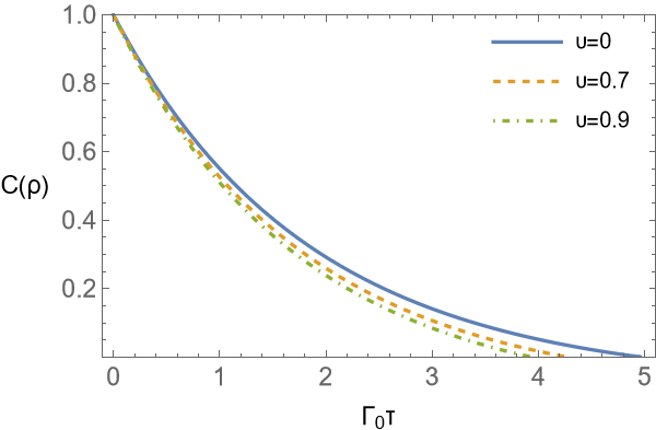
(a) $\beta\omega=5$ (UDW)

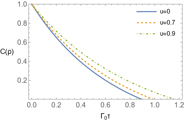
(b) $\beta\omega=1$ (UDW)

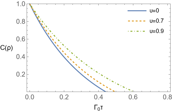
(c) $\beta\omega=0.5$ (UDW)

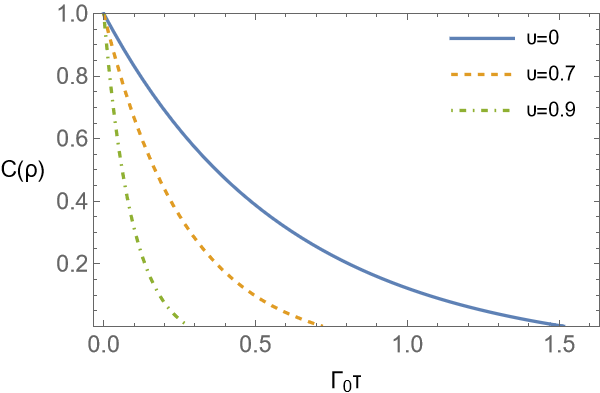
(d) $\beta\omega=5$ (TD)

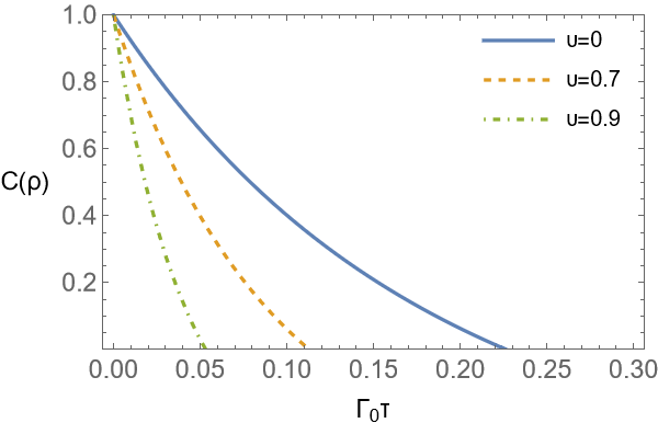
(e) $\beta\omega=1$ (TD)

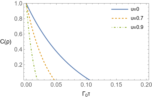
(f) $\beta\omega=0.5$ (TD)

Figure 1: Concurrence as a function of time (in units $\Gamma_{0}^{-1}$) in the UDW (upper) and the derivative coupling case (lower) respectively, for different detector velocities $\upsilon$ and temperatures $T=\beta^{-1}$ (in units of $\omega$) of the field bath. For the UDW coupling $\Gamma_{0}=\frac{\lambda^{2}\omega}{2\pi}$, whereas for the derivative coupling $\Gamma_{0}=\frac{\lambda^{2}\omega^{3}}{6\pi}$.

III Dynamics of entangled states

Motivated by [14, 15], we next introduce an identical two-level detector as an auxiliary system that is initially entangled with the moving detector. The auxiliary system is kept isolated from the field environment and does not interact with it.

The density matrix of the two-atom system is expressed in terms of the Pauli matrices as

$$\hat{\rho}(\tau)=\sum_{i=0}^{3}\sum_{j=0}^{3}u_{ij}(\tau)\hat{\sigma}_{i}\otimes\hat{\sigma}_{j},$$ (25)

where $u_{ij}=\frac{1}{4}\Tr(\rho\sigma_{i}\otimes\sigma_{j})$ are the components of the Bloch vector, and $\hat{\sigma}_{0}=\hat{1}$ denotes the identity operator. By substituting the density matrix (25) into the master equation (II.2) we obtain the following set of differential equations

$$\dot{u}_{0j}(\tau)= 0,$$

$$\dot{u}_{1j}(\tau)= -\frac{A}{2}u_{1j}(\tau)-\Omega u_{2j}(\tau),$$

$$\dot{u}_{2j}(\tau)= -\frac{A}{2}u_{2j}(\tau)+\Omega u_{1j}(\tau),$$

$$\dot{u}_{3j}(\tau)= -Au_{3j}(\tau)-Bu_{0j}(\tau)$$ (26)

for the coefficients $u_{ij}$, where for convenience we have defined $A:=\Gamma(2N+1),$ and $B:=-\Gamma$. Their solution reads

$$u_{0j}(\tau) =u_{0j}(0),$$

$$u_{1j}(\tau) =u_{1j}(0)e^{-\frac{A}{2}\tau}\cos(\Omega\tau)-u_{2j}(0)e^{-\frac{A}{2}\tau}\sin(\Omega\tau),$$

$$u_{2j}(\tau) =u_{1j}(0)e^{-\frac{A}{2}\tau}\sin(\Omega\tau)+u_{2j}(0)e^{-\frac{A}{2}\tau}\cos(\Omega\tau),$$

$$u_{3j}(\tau) =u_{3j}(0)e^{-A\tau}-u_{0j}(0)\frac{B}{A}\left(1-e^{-A\tau}\right).$$ (27)

We assume that initially the atoms are prepared in a maximally entangled Bell state

$$\hat{\rho}(0)=\frac{1}{4}(\hat{\sigma}_{0}\otimes\hat{\sigma}_{0}+\hat{\sigma}_{1}\otimes\hat{\sigma}_{1}-\hat{\sigma}_{2}\otimes\hat{\sigma}_{2}+\hat{\sigma}_{3}\otimes\hat{\sigma}_{3}),$$ (28)

that is the initial conditions $u_{00}(0)=u_{11}(0)=-u_{22}(0)=u_{33}(0)=1/4$ are applied. Thus, the evolution of the shared state between the moving atom and the auxiliary system is

$$\hat{\rho}(\tau)=\frac{1}{4}\Bigg{\{} \hat{\sigma}_{0}\otimes\hat{\sigma}_{0}+e^{-\frac{A}{2}\tau}\cos(\Omega\tau)(\hat{\sigma}_{1}\otimes\hat{\sigma}_{1}-\hat{\sigma}_{2}\otimes\hat{\sigma}_{2})$$

$$+e^{-\frac{A}{2}\tau}\sin(\Omega\tau)(\hat{\sigma}_{2}\otimes\hat{\sigma}_{1}+\hat{\sigma}_{1}\otimes\hat{\sigma}_{2})$$

$$+\frac{B}{A}(1-e^{-A\tau})\hat{\sigma}_{3}\otimes\hat{\sigma}_{0}+e^{-A\tau}\hat{\sigma}_{3}\otimes\hat{\sigma}_{3}\Bigg{\}}.$$ (29)

Our aim is to study how the amount of entanglement in the shared state (III) is affected by the motion of the one detector partner. To this end, we next calculate its concurrence.

III.1 Concurrence

To quantify the amount of entanglement present in an arbitrary two-qubit state $\rho$ we employ the concurrence [37, 38]

$$C(\rho)\equiv\text{max}\left(0,\lambda_{1}-\lambda_{2}-\lambda_{3}-\lambda_{4}\right),$$ (30)

where $\lambda_{i}$ are, in decreasing order, the square roots of eigenvalues of the matrix $R=\rho(\sigma_{y}\otimes\sigma_{y})\rho^{*}(\sigma_{y}\otimes\sigma_{y})$. Here, $\rho^{*}$ denotes the complex conjugate of $\rho$ and $\sigma_{y}$ is the usual Pauli matrix. Concurrence ranges from $C=0$ for a state with no entanglement to $C=1$ for a maximally entangled state.

We note that in the case of the so-called X-states [39, 40], which are characterized by the fact that their density matrix has non-zero elements along the main diagonal and anti-diagonal, i.e.,

$$\rho_{X}=\begin{pmatrix}\rho_{11}&0&0&\rho_{14}\\ 0&\rho_{22}&\rho_{23}&0\\ 0&\rho_{23}^{*}&\rho_{33}&0\\ \rho_{14}^{*}&0&0&\rho_{44}\end{pmatrix},$$ (31)

the concurrence is shown to be given by

$$C(\rho_{X})=2\,\text{max}\left(0,|\rho_{23}|-\sqrt{\rho_{11}\rho_{44}},|\rho_{14}|-\sqrt{\rho_{22}\rho_{33}}\right).$$ (32)

It can be easily shown that the state (III) is a X-state of the form (31). As a result, we can directly calculate concurrence by employing Eq. (32). We find that

$$C(\rho)=\max{\big{(}0,e^{-\frac{A}{2}\tau}-\frac{1-e^{-A\tau}}{2A}\sqrt{A^{2}-B^{2}}\big{)}}.$$ (33)

The concurrence (33) is plotted in Fig 1 as a function of time, in the case of the standard UDW (plots (a)-(c)) and derivative (plots (d)-(f)) coupling, for various velocities $\upsilon$ of the moving detector and temperatures $\beta^{-1}$ of the field bath. As may be expected, the initial amount of entanglement present in the shared state between the moving atom and its auxiliary partner monotonically decreases with time. In all cases, the rate of decrease becomes greater with the increase of the field bath temperature. Despite this, we can observe that in the UDW coupling model and for temperatures $\beta\leq\omega^{-1}$, entanglement loss is hindered when the atom is moving with a constant velocity. A greater delay of the entanglement degradation can be achieved with an increase of the atom's velocity. Thus, although the higher is the reservoir's temperature the greater the loss of an initial amount of entanglement, the latter can be delayed by making the detector to move along a worldine with constant velocity. Instead, this is not the case for the derivative coupling model, where the increase of the atom's velocity results in a substantial decrease of the concurrence.

The different environments are classified according to the form of their spectral density $J(\omega)$, which usually follows the power-law $J(\omega)\propto\omega^{\alpha}$ [26]. The most common choice for the exponent $\alpha$ is $\alpha=1$, in which case the the environment is characterized as Ohmic. If $\alpha<1$ the environment is characterized as subohmic, and if $\alpha>1$ as supraohmic respectively. We note that the massless scalar field bath $\hat{\phi}(\mathsf{x})$ represents an Ohmic environment (from Eq. (A) we have that $J(|\boldsymbol{k}|)\propto|\boldsymbol{k}|$), that is an environment whose spectral density is linear in frequency. Instead, when considering the derivative coupling case, the field bath $\dot{\hat{\phi}}(\mathsf{x})$ acts as a supraohmic environment. Thus, for higher values ($\beta\leq\omega^{-1}$) of temperature of an Ohmic environment, we conclude that an atom's motion can slow down the rate at which entanglement is lost, resulting in the preservation of entanglement for longer time. However, this is not true for supraohmic heat reservoirs: any interaction of moving atoms with them is always disastrous for entanglement.

Let us note finally that the time point at which entanglement completely disappears (i.e., $C(\rho)=0$) is given by the expression

$$\tau=-\frac{2}{A}\ln\left[\frac{-A+\sqrt{2A^{2}-B^{2}}}{\sqrt{A^{2}-B^{2}}}\right].$$ (34)

IV Concluding remarks

We demonstrated that by employing moving atoms we can decrease the rate at which entanglement is lost at high temperature Ohmic environments, consequently preserving entangled states for a longer period of time. Our result suggests the use of an atom's (relativistic) motion as a potential method to mitigate entanglement loss in quantum systems (although quantum entanglement is degraded in noninertial frames [43, 44]). Consequently, we highlight that except for the fact that concurrence is frame dependent [45], it also depends on the surrounding environment's characteristics. Besides, let us note that a similar to our result concerning quantum coherence was reported in [46, 47], where the authors show that the rate at which coherence is lost, is sometimes slower for a moving atom than for an atom at rest.

In future work, we aim to further explore the possibility of harnessing relativistic motion to counter entanglement loss in dissipative systems by studying the dynamics of entanglement between two spatially separated atoms that are both moving through a common thermal environment.

Entanglement harvesting protocols [48, 49, 50] are concerned with the extraction of entanglement that is inherently present in a quantum field onto two or more initially uncorrelated UDW detectors. Thus, apart from reducing decoherence, it would be also interesting to investigate how the inertial motion of atoms affect the process of harvesting entanglement (and mutual information) from thermal quantum fields [51]. We aim to tackle these questions in future work. Finally, the relation between entanglement generation and power of work extraction can be useful in quantum heat engines that take into account relativistic effects [52].

Appendix A Thermal two-point function

We next evaluate the two-point correlation function $\mathcal{W}(\mathsf{x},\mathsf{x}^{\prime})=\text{tr}(\hat{\rho}_{\beta}\hat{\phi}(\mathsf{x})\hat{\phi}(\mathsf{x}^{\prime}))$ of a massless scalar field in a thermal state $\hat{\rho}_{\beta}$. Employing the identity

$$\text{tr}\left(\hat{\rho}_{\beta}\hat{a}_{\boldsymbol{k}}^{\dagger}\hat{a}_{\boldsymbol{k}^{\prime}}\right)=\frac{1}{e^{\beta|\boldsymbol{k}|}-1}\delta^{(3)}(\boldsymbol{k}-\boldsymbol{k}^{\prime})$$ (35)

and the canonical commutation relations (2) we obtain

$$\text{tr}\Big{(}\hat{\rho}_{\beta}\hat{\phi}(\mathsf{x})\hat{\phi}(\mathsf{x}^{\prime})\Big{)}=\int\frac{d^{3}\boldsymbol{k}}{(2\pi)^{3}2|\boldsymbol{k}|}e^{-i|\boldsymbol{k}|(t-t^{\prime})}e^{i\boldsymbol{k}\cdot(\mathbf{x}-\mathbf{x}^{\prime})}$$

$$\quad+\int\frac{d^{3}\boldsymbol{k}}{(2\pi)^{3}2|\boldsymbol{k}|}\frac{1}{e^{\beta|\boldsymbol{k}|}-1}\left(e^{-i|\boldsymbol{k}|(t-t^{\prime})}e^{i\boldsymbol{k}\cdot(\mathbf{x}-\mathbf{x}^{\prime})}+\text{c.c.}\right).$$ (36)

Using spherical coordinates the Wightman function takes the form

$$\mathcal{W}(\mathsf{x},\mathsf{x}^{\prime})=\mathcal{W}_{\text{vac}}(\mathsf{x},\mathsf{x}^{\prime})$$

$$+\frac{1}{4\pi^{2}r}\int_{0}^{\infty}dk\,n_{k}\bigg{(}\sin\left(k(s+r)\right)-\sin\left(k(s-r)\right)\bigg{)},$$ (37)

where

$$\mathcal{W}_{\text{vac}}(\mathsf{x},\mathsf{x}^{\prime})=-\lim_{\epsilon\to 0^{+}}\frac{1}{4\pi^{2}}\frac{1}{(s-i\epsilon)^{2}-r^{2}}$$ (38)

is the vacuum two-point correlation function,

$$n_{k}=\frac{1}{e^{\beta|\boldsymbol{k}|}-1}$$ (39)

is the Planck distribution and we have set $s=t-t^{\prime}$ and $r=|\mathbf{x}-\mathbf{x}^{\prime}|$.

In the same way we obtain

$$\text{tr}\Big{(}\hat{\rho}_{\beta}\dot{\hat{\phi}}(\mathsf{x})\dot{\hat{\phi}}(\mathsf{x})\Big{)}=-\int\frac{d^{3}\boldsymbol{k}|\boldsymbol{k}|}{2(2\pi)^{3}}e^{-i|\boldsymbol{k}|(t-t^{\prime})}e^{i\boldsymbol{k}\cdot(\mathbf{x}-\mathbf{x}^{\prime})}$$

$$\quad-\int\frac{d^{3}\boldsymbol{k}|\boldsymbol{k}|}{2(2\pi)^{3}}\frac{1}{e^{\beta|\boldsymbol{k}|}-1}\left(e^{-i|\boldsymbol{k}|(t-t^{\prime})}e^{i\boldsymbol{k}\cdot(\mathbf{x}-\mathbf{x}^{\prime})}+\text{c.c.}\right),$$ (40)

which, bearing in mind Eq. (A), can equivalently be written as

$$\text{tr}\Big{(}\hat{\rho}_{\beta}\dot{\hat{\phi}}(\mathsf{x})\dot{\hat{\phi}}(\mathsf{x})\Big{)}=-\frac{\partial^{2}}{\partial s^{2}}\text{tr}\Big{(}\hat{\rho}_{\beta}\hat{\phi}(\mathsf{x})\hat{\phi}(\mathsf{x}^{\prime})\Big{)}.$$ (41)

References

- Horodecki et al. [2009] R. Horodecki, P. Horodecki, M. Horodecki, and K. Horodecki, Quantum entanglement, Rev. Mod. Phys. 81, 865 (2009).
- Bennett et al. [1993] C. H. Bennett, G. Brassard, C. Crépeau, R. Jozsa, A. Peres, and W. K. Wootters, Teleporting an unknown quantum state via dual classical and einstein-podolsky-rosen channels, Phys. Rev. Lett. 70, 1895 (1993).
- Bouwmeester et al. [1997] D. Bouwmeester, J.-W. Pan, K. Mattle, M. Eibl, H. Weinfurter, and A. Zeilinger, Experimental quantum teleportation, Nature (London) 390, 575 (1997), arXiv:1901.11004 [quant-ph] .
- Ekert [1991] A. K. Ekert, Quantum cryptography based on bell's theorem, Phys. Rev. Lett. 67, 661 (1991).
- Gisin et al. [2002] N. Gisin, G. Ribordy, W. Tittel, and H. Zbinden, Quantum cryptography, Rev. Mod. Phys. 74, 145 (2002).
- Bennett and Wiesner [1992] C. H. Bennett and S. J. Wiesner, Communication via one- and two-particle operators on einstein-podolsky-rosen states, Phys. Rev. Lett. 69, 2881 (1992).
- Nielsen and Chuang [2010] M. A. Nielsen and I. L. Chuang, Quantum Computation and Quantum Information: 10th Anniversary Edition (Cambridge University Press, 2010).
- Jozsa and Linden [2003] R. Jozsa and N. Linden, On the role of entanglement in quantum-computational speed-up, Proceedings of the Royal Society of London Series A 459, 2011 (2003), arXiv:quant-ph/0201143 [quant-ph] .
- Aolita et al. [2015] L. Aolita, F. de Melo, and L. Davidovich, Open-system dynamics of entanglement:a key issues review, Reports on Progress in Physics 78, 042001 (2015), arXiv:1402.3713 [quant-ph] .
- Viola et al. [1999] L. Viola, E. Knill, and S. Lloyd, Dynamical decoupling of open quantum systems, Phys. Rev. Lett. 82, 2417 (1999).
- Facchi et al. [2004] P. Facchi, D. A. Lidar, and S. Pascazio, Unification of dynamical decoupling and the quantum zeno effect, Phys. Rev. A 69, 032314 (2004).
- Maniscalco et al. [2008] S. Maniscalco, F. Francica, R. L. Zaffino, N. Lo Gullo, and F. Plastina, Protecting entanglement via the quantum zeno effect, Phys. Rev. Lett. 100, 090503 (2008).
- Lidar et al. [1998] D. A. Lidar, I. L. Chuang, and K. B. Whaley, Decoherence-free subspaces for quantum computation, Phys. Rev. Lett. 81, 2594 (1998).
- Doukas and Hollenberg [2009] J. Doukas and L. C. L. Hollenberg, Loss of spin entanglement for accelerated electrons in electric and magnetic fields, Phys. Rev. A 79, 052109 (2009).
- Tian and Jing [2014] Z. Tian and J. Jing, Dynamics and quantum entanglement of two-level atoms in de Sitter spacetime, Annals of Physics 350, 1 (2014), arXiv:1407.4930 [gr-qc] .
- Unruh [1976] W. G. Unruh, Notes on black-hole evaporation, Phys. Rev. D 14, 870 (1976).
- DeWitt [1979] B. S. DeWitt, Quantum gravity: The new synthesis, in General Relativity: an Einstein Centenary Survey, edited by S. Hawking and W. Israel (Cambridge University Press, Cambridge, England, 1979).
- Birrell and Davies [1982] N. D. Birrell and P. C. W. Davies, Quantum Fields in Curved Space (Cambridge University Press, Cambridge, England, 1982).
- Hu et al. [2012] B. L. Hu, S.-Y. Lin, and J. Louko, Relativistic quantum information in detectors-field interactions, Classical and Quantum Gravity 29, 224005 (2012).
- Hinton [1983] K. J. Hinton, Particle detectors in rindler and schwarzchild space-times, Journal of Physics A: Mathematical and General 16, 1937 (1983).
- Grove [1986] P. G. Grove, On the detection of particle and energy fluxes in two dimensions, Classical and Quantum Gravity 3, 793 (1986).
- Takagi [1986] S. Takagi, Vacuum Noise and Stress Induced by Uniform Acceleration: Hawking-Unruh Effect in Rindler Manifold of Arbitrary Dimension, Prog. Theor. Phys. Suppl. 88, 1 (1986).
- Juárez-Aubry and Louko [2014] B. A. Juárez-Aubry and J. Louko, Onset and decay of the 1 + 1 hawking-unruh effect: what the derivative-coupling detector saw, Classical and Quantum Gravity 31, 245007 (2014).
- Moustos [2018] D. Moustos, Asymptotic states of accelerated detectors and universality of the unruh effect, Phys. Rev. D 98, 065006 (2018).
- Scully and Zubairy [1997] M. O. Scully and M. S. Zubairy, Quantum Optics (Cambridge University Press, Cambridge, United Kingdom, 1997).
- Breuer and Petruccione [2007] H. P. Breuer and F. Petruccione, The Theory of Open Quantum Systems (Oxford University Press, New York, 2007).
- de Vega and Alonso [2017] I. de Vega and D. Alonso, Dynamics of non-markovian open quantum systems, Rev. Mod. Phys. 89, 015001 (2017).
- Moustos and Anastopoulos [2017] D. Moustos and C. Anastopoulos, Non-markovian time evolution of an accelerated qubit, Phys. Rev. D 95, 025020 (2017).
- Juárez-Aubry and Moustos [2019] B. A. Juárez-Aubry and D. Moustos, Asymptotic states for stationary unruh-dewitt detectors, Phys. Rev. D 100, 025018 (2019).
- Letaw [1981] J. R. Letaw, Stationary world lines and the vacuum excitation of noninertial detectors, Phys. Rev. D 23, 1709 (1981).
- Fleming et al. [2010] C. Fleming, N. I. Cummings, C. Anastopoulos, and B. L. Hu, The rotating-wave approximation: consistency and applicability from an open quantum system analysis, Journal of Physics A: Mathematical and Theoretical 43, 405304 (2010).
- Agarwal [1974] G. S. Agarwal, Quantum statistical theories of spontaneous emission and their relation to other approaches, in Springer Tracts in Modern Physics, Vol. 70 (1974) p. 1.
- Papadatos and Anastopoulos [2020] N. Papadatos and C. Anastopoulos, Relativistic quantum thermodynamics of moving systems, Phys. Rev. D 102, 085005 (2020).
- Lindblad [1976] G. Lindblad, On the generators of quantum dynamical semigroups, Communications in Mathematical Physics 48, 119 (1976).
- Gorini et al. [1976] V. Gorini, A. Kossakowski, and E. C. G. Sudarshan, Completely positive dynamical semigroups of N-level systems, Journal of Mathematical Physics 17, 821 (1976).
- Olver et al. [2010] F. W. Olver, D. W. Lozier, R. F. Boisvert, and C. W. Clark, NIST Handbook of Mathematical Functions (Cambridge University Press, USA, 2010).
- Hill and Wootters [1997] S. A. Hill and W. K. Wootters, Entanglement of a pair of quantum bits, Phys. Rev. Lett. 78, 5022 (1997).
- Wootters [1998] W. K. Wootters, Entanglement of formation of an arbitrary state of two qubits, Phys. Rev. Lett. 80, 2245 (1998).
- Yu and Eberly [2005] T. Yu and J. H. Eberly, Evolution from entanglement to decoherence of bipartite mixed "x" states, Quantum Inf. Comput. 7, 459 (2005), arXiv:0503089 [quant-ph] .
- Ali et al. [2010] M. Ali, A. R. P. Rau, and G. Alber, Quantum discord for two-qubit states, Phys. Rev. A 81, 042105 (2010).
- Schlicht [2004] S. Schlicht, Considerations on the unruh effect: causality and regularization, Classical and Quantum Gravity 21, 4647 (2004).
- Louko and Satz [2006] J. Louko and A. Satz, How often does the unruh–DeWitt detector click? regularization by a spatial profile, Classical and Quantum Gravity 23, 6321 (2006).
- Alsing et al. [2004] P. M. Alsing, D. McMahon, and G. J. Milburn, Teleportation in a non-inertial frame, Journal of Optics B: Quantum and Semiclassical Optics 6, S834 (2004).
- Alsing and Milburn [2003] P. M. Alsing and G. J. Milburn, Teleportation with a uniformly accelerated partner, Phys. Rev. Lett. 91, 180404 (2003).
- Gingrich and Adami [2002] R. M. Gingrich and C. Adami, Quantum entanglement of moving bodies, Phys. Rev. Lett. 89, 270402 (2002).
- Kollas et al. [2020] N. K. Kollas, D. Moustos, and K. Blekos, Field assisted extraction and swelling of quantum coherence for moving unruh-dewitt detectors, Phys. Rev. D 102, 065020 (2020).
- Kollas and Moustos [2022] N. K. Kollas and D. Moustos, Generation and catalysis of coherence with scalar fields, Phys. Rev. D 105, 025006 (2022).
- Valentini [1991] A. Valentini, Non-local correlations in quantum electrodynamics, Physics Letters A 153, 321 (1991).
- Reznik [2003] B. Reznik, Entanglement from the Vacuum, Foundations of Physics 33, 167 (2003), arXiv:quant-ph/0212044 [quant-ph] .
- Salton et al. [2015] G. Salton, R. B. Mann, and N. C. Menicucci, Acceleration-assisted entanglement harvesting and rangefinding, New Journal of Physics 17, 035001 (2015), arXiv:1408.1395 [quant-ph] .
- Simidzija and Martín-Martínez [2018] P. Simidzija and E. Martín-Martínez, Harvesting correlations from thermal and squeezed coherent states, Phys. Rev. D 98, 085007 (2018).
- Papadatos [2021] N. Papadatos, The Quantum Otto Heat Engine with a Relativistically Moving Thermal Bath, International Journal of Theoretical Physics 60, 4210 (2021), arXiv:2104.06611 [quant-ph] .