Breather solutions for a radially symmetric curl-curl wave equation with double power nonlinearity

Abstract

This paper is concerned with the breather solutions for a radially symmetric curl-curl wave equation with double power nonlinearity

$$\rho(x)\mathbf{u}_{tt}+\nabla\times(\mathbf{M}(x)\nabla\times\mathbf{u})+\mu(x)\mathbf{u}+v_{p}(x)|\mathbf{u}|^{p-1}\mathbf{u}+v_{q}(x)|\mathbf{u}|^{q-1}\mathbf{u}=0$$

where $(x,t)\in\mathbb{R}^{3}\times\mathbb{R}$, $\mathbf{u}:\mathbb{R}^{3}\times\mathbb{R}\rightarrow\mathbb{R}^{3}$ is the unknown function, $\mathbf{M}:\mathbb{R}^{3}\rightarrow\mathbb{R}^{3\times 3}$ and $\rho,\mu,v_{p},v_{q}:\mathbb{R}^{3}\rightarrow(0,+\infty)$ are radially symmetric coefficient functions, and $1<p<q$. By considering the solutions with a special form $\mathbf{u}=y(|x|,t)\frac{x}{|x|}$, we obtain a family of ordinary differential equations (ODEs) parameterized by the radial variable $r=|x|$. Then we use the qualitative analysis method of ODEs to characterize their periodic behaviors, and further analyze the joint effects of the double power nonlinear terms on the minimal period and the maximal amplitude. Finally, under the appropriate conditions on the coefficients, we construct a $2\pi\sqrt{\rho(0)/\mu(0)}$-periodic breather solution for the original curl-curl wave equation and find such a solution can generate a continuum of phase-shifted breathers.

1 Introduction

In this paper, we study the following radially symmetric curl-curl wave equation with double power nonlinearity

$$\rho(x)\mathbf{u}_{tt}+\nabla\times(\mathbf{M}(x)\nabla\times\mathbf{u})+\mu(x)\mathbf{u}+v_{p}(x)|\mathbf{u}|^{p-1}\mathbf{u}+v_{q}(x)|\mathbf{u}|^{q-1}\mathbf{u}=0$$ (1.1)

for $(x,t)\in\mathbb{R}^{3}\times\mathbb{R}$. Here $\mathbf{M}:\mathbb{R}^{3}\rightarrow\mathbb{R}^{3\times 3}$, and $\rho,\mu,v_{p},v_{q}:\mathbb{R}^{3}\rightarrow(0,\infty)$ are positive, radially symmetric functions with $v_{p}(x)=\left(\frac{\mu(x)^{q-p}}{v_{q}(x)^{1-p}}\right)^{\frac{1}{q-1}}$ and $1<p<q$. We consider the classical real-valued solutions $\mathbf{u}:\mathbb{R}^{3}\times\mathbb{R}\rightarrow\mathbb{R}^{3}$ which are $T$-periodic in time and spatially exponentially localized, i.e., sup${}_{\mathbb{R}^{3}\times\mathbb{R}}|\mathbf{u}(x,t)|e^{\gamma|x|}<\infty$ for some $\gamma>0$. The time periodic and spatially localized solutions are usually referred as breathers.

Breather solutions are of great significance in physics, biology and nonlinear optics, and attract extensive attentions of both mathematicians and physicists (see [2, 3, 10, 27]). It was first introduced by Ablowitz et al. [1] in the context of the (1+1)-dimensional sine-Gordon equation

$$u_{tt}-u_{xx}+\sin u=0\quad\mbox{in}\ \mathbb{R}\times\mathbb{R},$$

which possesses the breather families

$$u(x,t;\omega)=4\arctan\left(\frac{\sqrt{1-\omega^{2}}\cos(\omega t)}{\omega\cosh(\sqrt{1-\omega^{2}}x)}\right)$$

with $0<\omega<1$.

It is well known that breather solutions exist in various systems. For example, nonlinear wave equations and Schrödinger equations on discrete lattices can support breather solutions. MacKay and Aubry in [16] find that breather solutions exist in a broad range of time-reversible or Hamiltonian networks with small coupling constant. In [14], the existence of breathers are shown in some cases for any value of the coupling constant, which generalize the existence results obtained in [16]. In Schrödinger equations (see [5, 12, 15, 20, 21, 26]), the standing wave ansatz $u(x,t)=u(x)\exp(i\omega t)$ (see [28]) are usually very common tools to prove the existence of breathers. Comparing with the discrete cases, breathers in continuous cases are relatively difficult to obtain and have only a few results. Here, we pay more attention to breathers of nonlinear wave equations in continuous situations even many methods developed in discrete lattice systems are no longer applicable.

Our interest in breathers of the nonlinear wave equations originate from the fact that they cannot be observed in linear dispersion equations and are therefore a truly nonlinear phenomenon. We note that the family of breathers are nonpersistent under any nontrivial perturbation of sine-Gordon equation [7, 11]. By these works, it becomes clear that breathers do not exist in homogeneous nonlinear wave equations. For inhomogeneous nonlinear wave equations, the existence of breathers is a quite rare phenomenon. Blank et al. [8] use the spatial dynamics, center manifold theory and bifurcation theory construct such time periodic solutions with finite energy. It breaks the idea that the rescaled sine-Gordon equation is the only nonlinear wave equation which possesses breathers. Inspiringly, Hirsch et al. [13] consider a more general situation with $x$-dependent coefficients and include power-type nonlinearities like

$$\rho(x)u_{tt}-u_{xx}+\mu(x)u=\pm\Gamma(x)|u|^{p-1}u\quad\mbox{in}\ \mathbb{R}\times\mathbb{R},$$ (1.2)

where $\Gamma(x)$ is a $2\pi$-periodic continuous positive function and $1<p<p^{*}$ for some $p^{*}$ depend on the choice of $\rho(x)$ and $\mu(x)$. However, only the special case of $p=3$ is considered in [8]. Actually, we note that (1.2) is a special case of (1.1) with $\mathbf{M}$ represents the identity matrix and $v_{q}(x)=0$, and for solutions with the form

$$\mathbf{u}(x,t)=\begin{pmatrix}0\\ 0\\ u(x_{1},t)\end{pmatrix}.$$

A field of this form is divergence-free, i.e., div$\mathbf{u}$=0, and hence

$$\nabla\times\nabla\times\mathbf{u}(x,t)=\begin{pmatrix}0\\ 0\\ -\partial_{x_{1}}^{2}u(x_{1},t)\end{pmatrix}.$$

It is assumed in [8] and [13] that the potentials $\mu(x)$ is proportional to $\rho(x)$ which reduces the wave operator of the Fourier transform to a family of Hill-type ODE operators, thus the spectral analysis is significantly simplified. The authors in [13] choose the variational method so that the nonlinear term has no other smoothness assumptions except the continuity and superlinearity at $0$ and infinity. However, the above cases are only true in one dimensional space and it is difficult to generalize to higher spatial dimensions.

In fact, for higher dimensional nonlinear wave equations, there are few results on the existence of breather solutions. Recently, in [25], Scheider has constructed the weakly localized breathers by Fourier-expansion in time and bifurcation techniques for three dimensional case. For the spatial dimension $N\geq 2$, Mandel and Scheider in [17] obtain breather solutions that are also weakly localized in a distributional sense and polychromatic by dual variational method. It is entirely unclear whether strongly localized breathers of nonlinear wave equations exist in these cases. However, such strongly localized breather solutions which we are more interested play an important role in theoretical scenarios where photonic crystals are used as optical storage [9]. As far as we know, the only results dealing with strongly localized breathers of nonlinear wave equations in higher spatial dimensions is discussed in [23]. Inspired by the previous work, we intend to study a class of more general (3+1)-dimensional radially symmetric wave equations with double power nonlinearity involving curl-curl operators (possibly for the first time) and prove the existence of strongly localized breathers, i.e., $u(\cdot,t)\in C^{2}(\mathbb{R}^{3})$ for almost all $t\in\mathbb{R}$.

The particular feature curl-curl operator $\nabla\times(\mathbf{M}(x)\nabla\times)$ of (1.1) arises in specific models in the Maxwell equations as a physical motivation (see [4, 6, 18, 22]). In the absence of charges, currents and magnetization, we consider the Maxwell equations

$$\left\{\begin{matrix}\nabla\times\mathcal{H}=\partial_{t}\mathcal{D}\hfill\quad(\rm{Amp\grave{e}re^{\prime}s\ circuital\ law}),\\ \rm{div}(\mathcal{D})=0\hfill\quad(\rm{Gauss^{\prime}s\ law}),\\ \partial_{t}\mathcal{B}+\nabla\times\mathcal{E}=0\hfill\quad(\rm{Faraday^{\prime}s\ law\ of\ induction}),\\ \rm{div}(\mathcal{B})=0\hfill\quad(\rm{Gauss^{\prime}s\ law\ for\ magnetism}).\end{matrix}\right.$$ (1.3)

In such a medium, the constitutive relations between the electric displacement field $\mathcal{D}$ and the electric field $\mathcal{E}$ as well as between the magnetic field $\mathcal{H}$ and the magnetic induction $\mathcal{B}$ are given by

$$\mathcal{D}=\varepsilon\mathcal{E}+\mathcal{P}\quad\rm{and}\quad\mathcal{H}=\mathbf{M}\mathcal{B},$$ (1.4)

where $\varepsilon(x),\mathbf{M}(x)^{-1}:\mathbb{R}^{3}\rightarrow\mathbb{R}^{3\times 3}$ are the permittivity tensor and the permeability tensor of the anisotropic material, and $\mathcal{P}$ stands for the nonlinear polarization which depends nonlinearly on the electric field $\mathcal{E}$ and on the position $x\in\mathbb{R}^{3}$ in inhomogeneous media. The Maxwell equations (1.3) together with the constitutive relations (1.4) lead to the equation (see [24])

$$\nabla\times(\mathbf{M}(x)\nabla\times\mathcal{E})+\varepsilon(x)\partial_{t}^{2}\mathcal{E}=-\partial_{t}^{2}\mathcal{P}.$$ (1.5)

In a Kerr-like medium, one has $\mathcal{P}=\kappa(x)\langle|\mathcal{E}|^{2}\rangle\mathcal{E}$, where $\langle|\mathcal{E}|^{2}\rangle$ stands for the time average of the intensity of $\mathcal{E}$ (see [20, 29] for more details). In fact, we will be able to deal with more general polarization $\mathcal{P}$ in (1.5) which yields (1.1) with Kerr-like double power nonlinearities to model nonlinear phenomena.

Our interest in breathers under the context of the curl-curl nonlinear wave equations originates from the research for optical breathers of Maxwell’s equations in anisotropic materials where the permittivity depends nonlinearly on the electromagnetic fields (see [2]). However, the curl-curl operator exhibits major mathematical challenging. The main difficulty is that the $\nabla\times(\mathbf{M}(x)\nabla\times)$ operator has an infinite-dimensional kernel which causes the energy functional associated with (1.1) is strongly indefinite. To overcome these difficulties, Azzollini et al. [4] solve the curl-curl problems in $\mathbb{R}^{3}$ in the cylindrically symmetric setting, and then the method has been extensively used in the curl-curl problems related to the nonlinear Maxwell equations (see [6, 19] and references therein). However, we intend to take another completely different approach to deal with the difficulties which are caused by the curl-curl operator and find strongly localized real-valued breather solutions.

In this paper, we use the radially symmetric setting which makes heavy use of the particular spatial dependence of the coefficients, and the method is motivated by [6]. In this case, the gradient field is annihilated by the curl-curl operator due to the radially symmetric assumptions of the coefficients and a construction of the breathers. Then the (3+1)-dimensional wave equation reduces to a family of ordinary differential equations, which simplifies the problem considerably. Thus, by means of the ODEs technique, we characterize their periodic behaviors and further analyze the joint effects of the double power nonlinear terms on the minimal period and the maximal amplitude. We show the existence and extra exponential decay properties of real-valued breather solution of equation (1.1) in our two main theorems, which will be given in Section 4. As a side effect of our analysis, the solution we obtained can generate a continuum of phase-shifted breathers. Sometimes, monochromatic complex-valued waves of the type $\mathbf{u}(x,t)=\exp(i\omega t)\mathbf{u}(x)$ are also called breathers provided that $\mathbf{u}(x)$ decays to 0 as $|x|$ decays to $\infty$. In our present paper, we also prove the existence of breathers of the type $e^{i\frac{2\pi}{T}t}\mathbf{u}(x)$ under various assumptions on the coefficients in the second main theorem in Section 4 for the vector-valued wave equation (1.1).

This paper is organized as follows. In Section 2, we shall give some basic definitions and the construction of breather solutions, then obtain a family of ODEs possessing a first integral. In Section 3, we use the qualitative analysis method of the ODEs to characterize their periodic behaviors, and further analyze the joint effects of the double power nonlinear terms on the minimal period and the maximal amplitude. In Section 4, we will prove the two main theorems for the existence and extra exponential decay properties of breather solutions of (1.1). In Section 5, we give further conclusions of the overall picture of our results and discuss the outlook for the future that is possible due to the results.

2 Definitions and preliminaries

In this section, we give some basic definitions on $C^{2}$-function and the construction for breather solutions of (1.1). The gradient fields of radially symmetric functions are annihilated by the curl-curl operator. We eventually obtain a family of ODEs which can be reduced to a unified second-order differential equation possessing a first integral under some transformations.

Definition 2.1.

For a $C^{2}$-function $U:\mathbb{R}^{3}\rightarrow\mathbb{R}$, we say $U(x)\rightarrow 0$ in the $C^{2}$-sense as $x\rightarrow 0$, if

$$U(x)\rightarrow 0,\ \nabla U(x)\rightarrow 0,\ D^{2}U(x)\rightarrow 0\quad\mbox{as}\ x\rightarrow 0.$$

Definition 2.2.

For a radially symmetric $C^{2}$-function $U:\mathbb{R}^{3}\rightarrow\mathbb{R}$, let $\tilde{U}:[0,\infty)\rightarrow\mathbb{R}$ with $\tilde{U}(|x|)=U(x)$ be its one-dimensional representative, then we have $\tilde{U}\in C^{2}([0,\infty))$ and $\tilde{U}^{\prime}(0)=0$.

Lemma 2.1.

Let $\psi:[0,\infty)\rightarrow\mathbb{R}$ be a $C^{2}$-function and let $F:\mathbb{R}^{3}\setminus\left\{0\right\}\rightarrow\mathbb{R}^{3}$ be given by $F(x):=\psi(|x|)\frac{x}{|x|}$. Then $F$ can be extended to a function
(i) $F\in C^{1}(\mathbb{R}^{3})$ if and only if $\psi(0)=0$;
(ii) $F\in C^{2}(\mathbb{R}^{3})$ if and only if $\psi(0)=\psi^{\prime\prime}(0)=0$.

The proof of Lemma 2.1 refers to Lemma 1 in [23]. In what follows, we use functions $y=y(r,t)$ from $[0,\infty)\times\mathbb{R}$ to $\mathbb{R}$ with the notation ^′ to denote the differential form acting on the spatial variable and $\dot{}$ to denote the differential form acting on the time variable.

Under the radially symmetric assumptions of the coefficients in (1.1), we assume solutions $\mathbf{u}$ has the form

$$\mathbf{u}(x,t):=y(|x|,t)\frac{x}{|x|}$$

with

$$y(0,t)=y^{\prime\prime}(0,t)=0,$$

where $y:[0,\infty)\times\mathbb{R}\rightarrow\mathbb{R}$ is a $C^{2}$-function.

By Lemma 2.1, we can easily get $\mathbf{u}(x,t):=y(|x|,t)\frac{x}{|x|}$ is a $C^{2}(\mathbb{R}^{3}\times\mathbb{R})$ function of the variables $x$ and $t$, satisfying $\dot{y}(0,t)=\ddot{y}(0,t)=0$. Moreover, by the construction of $\mathbf{u}$, we obtain that it is a gradient-field, i.e., $\mathbf{u}(x,t)=\nabla_{x}Y(|x|,t)$ where $Y(r,t)=\int_{0}^{r}y(s,t)ds$. In this case we note that $\mathbf{M}(x)\nabla\times\mathbf{u}=0$ where $\mathbf{M}(x)\in\mathbb{R}^{3\times 3}$ is an arbitrary $3\times 3$ matrix function. Inserting the anstz of $\mathbf{u}(x,t)$ into (1.1) we obtain the following system

$$\tilde{\rho}(r)\ddot{y}+\tilde{\mu}(r)y+\tilde{v}_{p}(r)|y|^{p-1}y+\tilde{v}_{q}(r)|y|^{q-1}y=0\quad\mbox{for}\ r\geq 0,t\in\mathbb{R}.$$ (2.1)

Here we note that (2.1) is autonomous with respect to $t$ and that $r=|x|\geq 0$ is a parameter.

Since we intend to apply the ODEs technique to study breathers, let us find solutions $y(r,t)$ of (2.1) with the form

$$y(r,t)=\tau(r)\phi(\sigma(r)t).$$ (2.2)

Plugging this into (2.1) and comparing coefficients, we note that $\phi$ satisfies

$$\ddot{\phi}+\phi+|\phi|^{p-1}\phi+|\phi|^{q-1}\phi=0,$$ (2.3)

where we use

$$\sigma(r)=\left(\frac{\tilde{\mu}(r)}{\tilde{\rho}(r)}\right)^{\frac{1}{2}},\quad\tau(r)=\left(\frac{\tilde{\mu}(r)}{\tilde{v}_{q}(r)}\right)^{\frac{1}{q-1}},\quad\tilde{v}_{q}(r)=\left(\frac{\tilde{\mu}(r)^{p-q}}{\tilde{v}_{p}(r)^{1-q}}\right)^{\frac{1}{p-1}}.$$ (2.4)

By multiplying the left and right ends of (2.3) by $2\dot{\phi}$, it is easy to obtain that

$$\dot{\phi}^{2}+\phi^{2}+\frac{2}{p+1}|\phi|^{p+1}+\frac{2}{q+1}|\phi|^{q+1}=c$$

for some constant $c\in[0,\infty)$.

Definition 2.3.

Define the function $B:\mathbb{R}^{2}\rightarrow\mathbb{R}$ by

$$B(\alpha,\beta):=\beta^{2}+\alpha^{2}+\frac{2}{p+1}|\alpha|^{p+1}+\frac{2}{q+1}|\alpha|^{q+1}.$$ (2.5)

Then $B$ is a first integral for (2.3), i.e., every solution $\phi$ of (2.3) satisfies $B(\phi,\dot{\phi})=c$.

We note that every orbit of (2.3) is uniquely characterized by the value $c\in[0,\infty)$, then we use the qualitative analysis method of ODEs to characterize their periodic behaviors in next section.

3 Qualitative analysis

In what follows, with the help of the first integral (2.5) and by using the qualitative analysis method of ODEs, we characterize the periodic behaviors of solutions of equation (2.3), and further analyze the joint effects of the double nonlinear terms on the minimal period $P(c)$ and the maximal amplitude $A(c):=\max_{t\in\mathbb{R}}|\phi(t)|$ for every orbit of (2.3). Here we give some useful lemmas.

Lemma 3.1.

$A(c)$ enjoys the following properties:

$(1)$ $A\in C([0,\infty))\bigcap C^{\infty}(0,\infty)$ and $A([0,\infty))=[0,\infty)$;

$(2)$ $A^{\prime}(c)>0$ and $A(c)\leq\sqrt{c}$ for all $c>0$;

$(3)$ $\lim_{c\rightarrow 0}\frac{A(c)}{\sqrt{c}}=1$ and $\lim_{c\rightarrow\infty}A(c)=\infty$.

Proof.

The maximal amplitude $A(c)$ is given by

$$B(A(c),0)=A(c)^{2}+\frac{2}{p+1}A(c)^{p+1}+\frac{2}{q+1}A(c)^{q+1}=c,$$ (3.1)

which implies the strict continuity, monotonicity and differentiability of $A(c)$ with respect to $c>0$. It also provides the inequality $A(c)\leq\sqrt{c}$ since $A(c)^{2}\leq c$ and $A(c)\geq 0$. Moreover, we have $\lim_{c\rightarrow 0}\frac{A(c)}{\sqrt{c}}=1$ and $\lim_{c\rightarrow\infty}A(c)=\infty$ by (3.1). This completes the proof. ∎

Lemma 3.2.

$P(c)$ enjoys the following properties:

$(1)$ $P\in C([0,\infty))\bigcap C^{\infty}((0,\infty))$ and $P([0,\infty))=(0,2\pi]$;

$(2)$ $\lim_{c\rightarrow\infty}P(c)=0$ and $P(0)=2\pi$.

Proof.

We verify the statements for $P(c)$ by using the first integral

$$|\dot{\phi}|^{2}+|\phi|^{2}+\frac{2}{p+1}|\phi|^{p+1}+\frac{2}{q+1}|\phi|^{q+1}=c$$

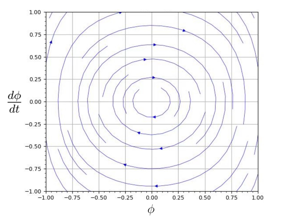
Figure 1: Part of the phase plane of (2.3) for p=4 and q=8.

to solve for $\dot{\phi}$ in all four quadrants of the phase-plane, cf. Figure 1. The function $P(c)$ is given implicitly through the defining equation (3.1) of $A(c)$, which yields

$$P(c) = 4\int_{0}^{A(c)}\frac{1}{\sqrt{c-\phi^{2}-\frac{2}{p+1}\phi^{p+1}-\frac{2}{q+1}\phi^{q+1}}}d\phi$$ (3.2)

$$= 4\int_{0}^{1}\frac{A(c)}{\sqrt{c-A(c)^{2}z^{2}-\frac{2}{p+1}A(c)^{p+1}z^{p+1}-\frac{2}{q+1}A(c)^{q+1}z^{q+1}}}dz$$

$$= 4\int_{0}^{1}\frac{1}{\sqrt{1-z^{2}+\frac{2}{p+1}A(c)^{p-1}(1-z^{p+1})+\frac{2}{q+1}A(c)^{q-1}(1-z^{q+1})}}dz.~{}~{}~{}~{}~{}~{}$$

It shows that $P(c)$ has the asserted smoothness. From Lemma 3.1, we also find that $\lim_{c\rightarrow\infty}P(c)=0$ and

$$\lim_{c\rightarrow 0}P(c)=4\int_{0}^{1}\frac{1}{\sqrt{1-z^{2}}}dz=2\pi.$$

The proof is completed. ∎

Lemma 3.3.

$P(c)$ is invertible and its inverse $Q=P^{-1}:(0,2\pi]\rightarrow[0,\infty)$ is $C^{\infty}$ on $(0,2\pi)$ and has the following expansions as $s\rightarrow 2\pi^{-}$

$$Q(s) = \lambda(2\pi-s)^{\frac{2}{q-1}}(1+O(2\pi-s)),$$

$$\sqrt{Q(s)} = \sqrt{\lambda}(2\pi-s)^{\frac{1}{q-1}}(1+O(2\pi-s)),$$

$$Q^{\prime}(s) = -\frac{2\lambda}{q-1}(2\pi-s)^{\frac{3-q}{q-1}}(1+O(2\pi-s)),$$

$$\sqrt{Q(s)}^{\prime} = -\frac{\sqrt{\lambda}}{q-1}(2\pi-s)^{\frac{2-q}{q-1}}(1+O(2\pi-s)),$$

$$Q^{\prime\prime}(s) = \frac{2\lambda(3-q)}{(q-1)^{2}}(2\pi-s)^{\frac{4-2q}{q-1}}(1+O(2\pi-s)),$$

$$\sqrt{Q(s)}^{\prime\prime} = \frac{\sqrt{\lambda}(2-q)}{(q-1)^{2}}(2\pi-s)^{\frac{3-2q}{q-1}}(1+O(2\pi-s))$$

for some constant $\lambda>0$.

Proof.

From (3.2), we define

$$P(c)=W\left(\frac{2}{q+1}A(c)^{q-1}\right),$$

where

$$W(u) = 4\int_{0}^{1}\frac{1}{\sqrt{1-z^{2}+\frac{2}{p+1}(1-z^{p+1})(\frac{q+1}{2})^{\frac{p-1}{q-1}}u^{\frac{p-1}{q-1}}+u(1-z^{q+1})}}dz$$

$$= 4\int_{0}^{1}\frac{1}{\sqrt{1-z^{2}}\sqrt{1+m(z)\left(u+\frac{2}{p+1}(\frac{q+1}{2})^{\frac{p-1}{q-1}}u^{\frac{p-1}{q-1}}n(z)\right)}}dz,$$

with $u=\frac{2}{q+1}A(c)^{q-1}\geq 0$, $m(z)=\frac{1-z^{q+1}}{1-z^{2}}$ and $n(z)=\frac{1-z^{p+1}}{1-z^{q+1}}$ are continuous and positive functions on $[0,1]$ and $[1,\infty)$ respectively. We note that $W(0)=2\pi$, $W(\infty)=0$, $W\in C^{\infty}[0,\infty)$ and $W$ is strictly decreasing and convex since

$$W^{\prime}(u) =\ -2\int_{0}^{1}\frac{m(z)\left(1+\frac{2(p-1)}{(p+1)(q-1)}(\frac{q+1}{2})^{\frac{p-1}{q-1}}u^{\frac{p-q}{q-1}}n(z)\right)}{\sqrt{1-z^{2}}\left(1+m(z)\left(u+\frac{2}{p+1}(\frac{q+1}{2})^{\frac{p-1}{q-1}}u^{\frac{p-1}{q-1}}n(z)\right)\right)^{\frac{3}{2}}}dz$$ (3.3)

$$=: -2\int_{0}^{1}\frac{h(u,z)}{\sqrt{1-z^{2}}g(u,z)^{\frac{3}{2}}}dz<0$$

for $1<p<q$, and

$$W^{\prime\prime}(u) = -2\int_{0}^{1}\frac{h^{\prime}(u,z)g(u,z)^{\frac{3}{2}}-h(u,z)\frac{3}{2}g(u,z)^{\frac{1}{2}}h(u,z)}{\sqrt{1-z^{2}}g(u,z)^{3}}dz$$

$$= -2\int_{0}^{1}\frac{m(z)\frac{2(p-1)(p-q)}{(p+1)(q-1)^{2}}(\frac{q+1}{2})^{\frac{p-1}{q-1}}u^{\frac{p-2q+1}{q-1}}g(u,z)-\frac{3}{2}h(u,z)^{2}}{\sqrt{1-z^{2}}g(u,z)^{\frac{5}{2}}}dz>0.$$

Thus we obtain $W^{-1}\in C^{\infty}((0,2\pi])$. Furthermore, by (3.3) and the fact that $A^{\prime}(c)>0$ on $(0,\infty)$, it is obviously that $P^{\prime}(c)<0$ on $(0,\infty)$ which implies the invertibility of $P$.

We then study $P^{-1}$ for some preparations. With the defining equation (3.1) for $A(c)$ and $u=\frac{2}{q+1}A(c)^{q-1}$, we have

$$c =\ A(c)^{2}+\frac{2}{p+1}A(c)^{p+1}+\frac{2}{q+1}A(c)^{q+1}$$

$$=\ (\frac{q+1}{2})^{\frac{2}{q-1}}(u^{\frac{2}{q-1}}+u^{\frac{q+1}{q-1}})+\frac{2}{p+1}(\frac{q+1}{2})^{\frac{p+1}{q-1}}u^{\frac{p+1}{q-1}}$$

$$=: \Psi(u).$$

Then we denote

$$P(c)=W(u)=W(\Psi^{-1}(c))\quad\mbox{and}\quad Q=P^{-1}=\Psi\circ W^{-1}.$$

From Taylor approximation for $W^{-1}$ at $2\pi$ with $\tilde{\lambda}=-\frac{1}{W^{\prime}(0)}>0$, $\tilde{\theta}=W^{\prime\prime}(0)>0$, we find that as $s\rightarrow 2\pi^{-}$

$$W^{-1}(s) = W^{-1}(2\pi)+(W^{-1})^{\prime}(2\pi)(s-2\pi)+O((2\pi-s)^{2})$$

$$= \tilde{\lambda}(2\pi-s)(1+O(2\pi-s)),$$

$$(W^{-1})^{\prime}(s) = \frac{1}{W^{\prime}(W^{-1}(s))}=-\tilde{\lambda}(1+O(2\pi-s)),$$

$$(W^{-1})^{\prime\prime}(s) = -\frac{W^{\prime\prime}(W^{-1}(s))}{\left(W^{\prime}(W^{-1}(s))\right)^{3}}=\tilde{\theta}\tilde{\lambda}^{3}(1+O(2\pi-s)).$$

Thus, as $s\rightarrow 2\pi^{-}$ we obtain

$$Q(s) = \Psi(W^{-1}(s))$$

$$= (\frac{q+1}{2})^{\frac{2}{q-1}}\left((W^{-1}(s))^{\frac{2}{q-1}}+(W^{-1}(s))^{\frac{q+1}{q-1}}\right)$$

$$+\frac{2}{p+1}(\frac{q+1}{2})^{\frac{p+1}{q-1}}(W^{-1}(s))^{\frac{p+1}{q-1}}$$

$$= \lambda(2\pi-s)^{\frac{2}{q-1}}(1+O(2\pi-s))$$

with $\lambda=(\frac{q+1}{2})^{\frac{2}{q-1}}\tilde{\lambda}^{\frac{2}{q-1}}>0$. Note that

$$Q^{\prime}(s) = \Psi^{\prime}(W^{-1}(s))(W^{-1})^{\prime}(s))$$

$$= (\frac{q+1}{2})^{\frac{2}{q-1}}\left(\frac{2}{q-1}(W^{-1}(s))^{\frac{3-q}{q-1}}+\frac{q+1}{q-1}(W^{-1}(s))^{\frac{2}{q-1}}\right)$$

$$\times(-\tilde{\lambda})(1+O(2\pi-s))$$

$$+\frac{2}{q-1}(\frac{q+1}{2})^{\frac{p+1}{q-1}}(W^{-1}(s))^{\frac{p-q+2}{q-1}}(-\tilde{\lambda})(1+O(2\pi-s))$$

$$= -\frac{2\lambda}{q-1}(2\pi-s)^{\frac{3-q}{q-1}}(1+O(2\pi-s))$$

and

$$Q^{\prime\prime}(s) = \Psi^{\prime\prime}(W^{-1}(s))\left((W^{-1})^{\prime}(s)\right)^{2}+\Psi^{\prime}(W^{-1}(s))(W^{-1})^{\prime\prime}(s)$$

$$= (\frac{q+1}{2})^{\frac{2}{q-1}}\left(\frac{2(3-q)}{(q-1)^{2}}(W^{-1}(s))^{\frac{4-2q}{q-1}}+\frac{2(q+1)}{(q-1)^{2}}(W^{-1}(s))^{\frac{3-q}{q-1}}\right)$$

$$\times\tilde{\lambda}^{2}(1+O(2\pi-s))$$

$$+\frac{2(p-q+2)}{(q-1)^{2}}(\frac{q+1}{2})^{\frac{p+1}{q-1}}(W^{-1}(s))^{\frac{p-2q+3}{q-1}}\tilde{\lambda}^{2}(1+O(2\pi-s))$$

$$+O((2\pi-s)^{\frac{3-q}{q-1}})$$

$$= \frac{2\lambda(3-q)}{(q-1)^{2}}(2\pi-s)^{\frac{4-2q}{q-1}}(1+O(2\pi-s)).$$

The representations for $\sqrt{Q}$, $\sqrt{Q}^{\prime}=\frac{Q^{\prime}}{2\sqrt{Q}}$ and $\sqrt{Q}^{\prime\prime}=\frac{1}{2Q^{3/2}}(Q^{\prime\prime}Q-\frac{1}{2}(Q^{\prime})^{2})$ follow directly from the representations of $Q$, $Q^{\prime}$ and $Q^{\prime\prime}$. The proof is completed. ∎

4 Main results

In this section, we will give the two main theorems for the existence results on the breathers in (1.1) and their corresponding proofs.

Theorem 4.1.

Suppose $\rho(x),\mu(x),v_{p}(x),v_{q}(x):\mathbb{R}^{3}\rightarrow(0,\infty)$ are radially symmetric $C^{2}$-functions and let $T=2\pi\sqrt{\frac{\rho(0)}{\mu(0)}}$. Assume

$(H1)$ $T\sqrt{\frac{\mu(x)}{\rho(x)}}<2\pi$ for all $x\in\mathbb{R}^{3}\setminus\{0\}$,

$(H2)$ $|2\pi-T\sqrt{\frac{\mu(x)}{\rho(x)}}|^{\frac{1}{q-1}}\rightarrow 0$ in the $C^{2}$-sense as $x\rightarrow 0$,

$(H3)$ $\sup_{x\in\mathbb{R}^{3}}|2\pi-T\sqrt{\frac{\mu(x)}{\rho(x)}}|e^{\gamma(q-1)|x|}<\infty$ for some $\gamma>0$,

$(H4)$ $\sup_{x\in\mathbb{R}^{3}}\frac{\mu(x)}{v_{q}(x)}<\infty$.
Thus there exists a $T$-periodic $\mathbb{R}^{3}$-valued breather solution $\mathbf{u}$ of (1.1) with the extra property that $\sup_{\mathbb{R}^{3}\times\mathbb{R}}|\mathbf{u}(x,t)|e^{\gamma|x|}<\infty$. The breather $\mathbf{u}$ generates a continuum of phase-shifted breathers $\mathbf{u}_{b}(x,t)=\mathbf{u}(x,t+b(x))$ where $b:\mathbb{R}^{3}\rightarrow\mathbb{R}$ is an arbitrary radially symmetric $C^{2}$-function.

Proof.

We first select a $C^{2}$-curve $\xi:[0,\infty)\rightarrow\mathbb{R}^{2}$ in the phase space so that $B(\xi(c))=c^{2}$, where $B$ is the first integral from Definition 2.3. Then let us give an example to make it easier to understand such a curve, i.e., $\xi(c)=(0,c)$, which only selects a special case of the continuum of phase-shifted breathers as described. However there exist some other choices of $\xi$ and will be given later.

We denote the solution of (2.3) by $\phi(t;c)$ with $(\phi(0;c),\dot{\phi}(0;c))=\xi(c)$. Then $\phi:\mathbb{R}\times[0,\infty)\rightarrow\mathbb{R}$ is a $C^{2}$-function and $\phi(t;c)$ is $P(c^{2})$-periodic in the $t$-variable. Now let us define the solution $y$ of (2.1) by

$$y(r,t)=\tau(r)\phi(\sigma(r)t;c)$$ (4.1)

with

$$\sigma(r)=\left(\frac{\tilde{\mu}(r)}{\tilde{\rho}(r)}\right)^{\frac{1}{2}},\ \ \tau(r)=\left(\frac{\tilde{\mu}(r)}{\tilde{v}_{q}(r)}\right)^{\frac{1}{q-1}},\ \ \tilde{v}_{q}(r)=\left(\frac{\tilde{\mu}(r)^{p-q}}{\tilde{v}_{p}(r)^{1-q}}\right)^{\frac{1}{p-1}}$$ (4.2)

as described in (2.4). The requirement of $T$-periodicity of $y$ in the $t$-variable tells us how to choose $c$ as a function of the radial variable $r\in[0,\infty)$, i.e.,

$$d(r):=\sigma(r)T=P(c^{2}).$$ (4.3)

We recall that $Q=P^{-1}$ and $Q:(0,2\pi]\rightarrow[0,\infty)$ is strictly decreasing and $C^{\infty}$ on $(0,2\pi)$ (see Lemmas 3.2 and 3.3). Then

$$c(r)=\sqrt{Q(d(r))}$$ (4.4)

can be inserted into (4.1). We find that $c(r)$ is well-defined and $C^{2}$ on $(0,\infty)$ by the assumption $(H1)$. In order to apply the assuming form $\mathbf{u}(x,t):=y(|x|,t)\frac{x}{|x|}$, we need to prove $y:[0,\infty)\times\mathbb{R}\rightarrow\mathbb{R}$ is a $C^{2}$-function and $y(0,t)=y^{\prime\prime}(0,t)=0$. First we prove that $y(r,t)$ tends to 0 as $r\rightarrow 0$ and even exponentially decays to 0 as $r\rightarrow 0$. Note that

$$|y(r,t)| \leq \left(\frac{\tilde{\mu}(r)}{\tilde{v}_{q}(r)}\right)^{\frac{1}{q-1}}A(c(r)^{2})$$

$$\leq \left(\frac{\tilde{\mu}(r)}{\tilde{v}_{q}(r)}\right)^{\frac{1}{q-1}}c(r)$$

$$\leq G\sqrt{Q(d(r))},$$

by Lemma 3.1 and the assumption $(H4)$, where $G$ is a constant. The assumptions $(H2)$ and $(H3)$ yield that $d(r)$ tends to $2\pi$ as $r\rightarrow\infty$ and as $r\rightarrow 0$, then we have the estimate

$$|y(r,t)|\leq G\sqrt{\lambda}(2\pi-d(r))^{\frac{1}{q-1}}O(1)\quad\mbox{as}\ r\rightarrow\infty\ \mbox{and}\ \mbox{as}\ r\rightarrow 0.$$ (4.5)

By the assumption $(H3)$, we obtain that $|y(r,t)|\leq Ce^{-\gamma r}$ for $r\geq 0$, with some positive constant $C$. It implies the exponential decay of $\mathbf{u}(x,t)=y(|x|,t)\frac{x}{|x|}$ as $|x|\rightarrow\infty$.

By (4.5) and the assumption $(H2)$, we have $y(0,t)=0$, then we only need to prove $y^{\prime\prime}(0,t)=0$. For this, by (4.4) we have

$$c(r)=\sqrt{\lambda}(2\pi-d(r))^{\frac{1}{q-1}}O(1)\rightarrow 0\quad\mbox{as}\ r\rightarrow 0.$$

Furthermore, by Lemma 3.3 and the assumption $(H2)$, we have

$$c^{\prime}(r) = \sqrt{Q}^{\prime}(d(r))d^{\prime}(r)$$

$$= -\frac{\sqrt{\lambda}}{q-1}(2\pi-d(r))^{\frac{2-q}{q-1}}O(1)d^{\prime}(r)$$

$$= \sqrt{\lambda}\left((2\pi-d(r))^{\frac{1}{q-1}}\right)^{\prime}O(1)$$

$$= o(1)\ \ as\ r\rightarrow 0.$$

Moreover,

$$c^{\prime\prime}(r) = \sqrt{Q}^{\prime\prime}(d(r))d^{\prime}(r)^{2}+\sqrt{Q}^{\prime}(d(r))d^{\prime\prime}(r)$$

$$= \frac{\sqrt{\lambda}(2-q)}{(q-1)^{2}}(2\pi-d(r))^{\frac{3-2q}{q-1}}(1+O(2\pi-d(r)))d^{\prime}(r)^{2}$$

$$-\frac{\sqrt{\lambda}}{q-1}(2\pi-d(r))^{\frac{2-q}{q-1}}(1+O(2\pi-d(r)))d^{\prime\prime}(r)$$

$$= \sqrt{\lambda}\left((2\pi-d(r))^{\frac{1}{q-1}}\right)^{\prime\prime}+O(1)\frac{\sqrt{\lambda}(2-q)}{(q-1)^{2}}(2\pi-d(r))^{\frac{2-q}{q-1}}d^{\prime}(r)^{2}$$

$$-O(1)\frac{\sqrt{\lambda}}{q-1}(2\pi-d(r))^{\frac{1}{q-1}}d^{\prime\prime}(r).$$

The term $L_{1}(r)=\left((2\pi-d(r))^{\frac{1}{q-1}}\right)^{\prime\prime}\rightarrow 0$ as $r\rightarrow 0$ by the assumption $(H2)$. By the definition of $d(r)$, we obtain that $d$ is a $C^{2}$-function on $[0,\infty)$. Thus the term $L_{2}(r)=(2\pi-d(r))^{\frac{2-q}{q-1}}d^{\prime}(r)^{2}=(1-q)\left((2\pi-d(r))^{\frac{1}{q-1}}\right)^{\prime}d^{\prime}(r)\rightarrow 0$ as $r\rightarrow 0$, since $d^{\prime}$ is bounded near 0 and the assumption $(H2)$. As for the term $L_{3}=(2\pi-d(r))^{\frac{1}{q-1}}d^{\prime\prime}(r)$, it converges to 0 since $d(r)\rightarrow 2\pi$ as $r\rightarrow 0$ and $d^{\prime\prime}$ is bounded near 0. Then the above equation implies $c^{\prime\prime}(r)\rightarrow 0$ as $r\rightarrow 0$. So that $c$ can be extended to a function $c\in C^{2}([0,\infty))$ with $c(0)=c^{\prime}(0)=c^{\prime\prime}(0)=0$. From this and (4.1), we have $y(r,t)\in C^{2}([0,\infty)\times\mathbb{R})$ with the presentation $y(r,t)=\tau(r)\phi(\sigma(r)t,c)$. Then we compute

$$y^{\prime}(r,t)=\tau^{\prime}(r)\phi(\sigma(r)t,c(r))+\tau(r)\dot{\phi}(\sigma(r)t,c(r))\sigma^{\prime}(r)t+\tau(r)\frac{\partial\phi}{\partial c}(\sigma(r)t,c(r))c^{\prime}(r)$$

and

$$y^{\prime\prime}(0,t) = \tau^{\prime\prime}(0)\phi(\sigma(0)t,c(0))+2\tau^{\prime}(0)\dot{\phi}(\sigma(0)t,c(0))\sigma^{\prime}(0)t$$

$$+2\tau^{\prime}(0)\frac{\partial\phi}{\partial c}(\sigma(0)t,c(0))c^{\prime}(0)+\tau(0)\ddot{\phi}(\sigma(0)t,c(0))\sigma^{\prime}(0)^{2}t^{2}$$

$$+\tau(0)\dot{\phi}(\sigma(0)t,c(0))\sigma^{\prime\prime}(0)t+2\tau(0)\frac{\partial\dot{\phi}}{\partial c}(\sigma(0)t,c(0))\sigma^{\prime}(0)tc^{\prime}(0)$$

$$+\tau(0)\frac{\partial^{2}\phi}{\partial c^{2}}(\sigma(0)t,c(0))c^{\prime}(0)^{2}+\tau(0)\frac{\partial\phi}{\partial c}(\sigma(0)t,c(0))c^{\prime\prime}(0)$$

$$= 0,$$

where we use $\phi(\cdot,0)=0$, $\dot{\phi}(\cdot,0)=0$, $\ddot{\phi}(\cdot,0)=0$ and $c(0)=c^{\prime}(0)=c^{\prime\prime}(0)=0$. By Lemma 2.1, this means that $\mathbf{u}(x,t)\in C^{2}(\mathbb{R}^{3}\times\mathbb{R})$.

Next, we will show how to generate a continuum of different phase-shifted breathers from a radially symmetric breather solution.

First we discuss the choice of the initial curve $\xi(c)=(0,c)$ which give rise to the solution family $\phi(t;c)$ such that $(\phi(0;c),\dot{\phi}(0;c))=\xi(c)$. Our purpose is to find some $C^{2}$-curve such that $B(\xi(c))=c^{2}$. The special selection $\xi(c)=(0,c)$ is convenient but arbitrary. Then other possible choices of $\xi$ will be given, for example, by

$$\tilde{\xi}(c):=(\phi(a(c);c),\dot{\phi}(a(c);c)),$$

where $a(c)$ is an arbitrary real $C^{2}$-function on $[0,\infty)$. It is obviously that $B(\tilde{\xi}(c))=B(\phi(a(c);c),\dot{\phi}(a(c);c))=c^{2}$, where $B$ is the first integral of (2.3). As for the new curve $\tilde{\xi}(c)$, we can give a new solution family $\tilde{\phi}(t;c)$ determined by the initial conditions

$$(\tilde{\phi}(0;c),\dot{\tilde{\phi}}(0;c))=\tilde{\xi}(c).$$

By the uniqueness of the initial value problem, the above two solution families have a simple relationship as

$$\tilde{\phi}(t;c)=\phi(t+a(c);c).$$

In order to see the effect of the choice of the new curve, we compare the solutions $\mathbf{u}$ and $\tilde{\mathbf{u}}$ generated by $\xi$ and $\tilde{\xi}$, i.e.,

$$\mathbf{u}(x,t)=\tau(r)\phi(\sigma(r)t;c(r))\frac{x}{|x|}$$

with $c(r)=\sqrt{Q(d(r))}=\sqrt{P^{-1}(\sigma(r)T)}$ and

$$\tilde{\mathbf{u}}(x,t) = \tau(r)\tilde{\phi}(\sigma(r)t;c(r))\frac{x}{|x|}$$

$$= \tau(r)\phi(\sigma(r)t+a(c(r));c(r))\frac{x}{|x|}$$

$$= y(|x|,t+\tilde{b}(r))\frac{x}{|x|}$$

$$= \mathbf{u}(x,t+\tilde{b}(r)),$$

where $\tilde{b}(r)=a(c(r))/\sigma(r)$ is a $C^{2}$-function on $[0,\infty)$. Then $b:\mathbb{R}^{3}\rightarrow\mathbb{R}$ is an arbitrary radially symmetric $C^{2}$-function generated by $b(x)=\tilde{b}(|x|)$ as described in Theorem 4.1. Thus the different choice of the initial curve can generate a continuum of phase-shifted breathers from one radially symmetric breather solution. This completes the proof of this theorem. ∎

Remark 4.1.

Let $\mu(x)=2|x|^{2}+1,\rho(x)=\frac{2|x|^{2}+1}{(1-|x|^{4}e^{-|x|^{4}})^{2}},v_{q}(x)=|x|^{2}e^{|x|^{2}}+1$. By a simple computation, it is easy to check that these functions satisfy the assumptions $(H1)-(H4)$. In this case, we can prove that the $2\pi$-periodic $\mathbb{R}^{3}$-valued breather solution exists in Theorem 4.1 and it can be exhibited, cf. Figure 2.

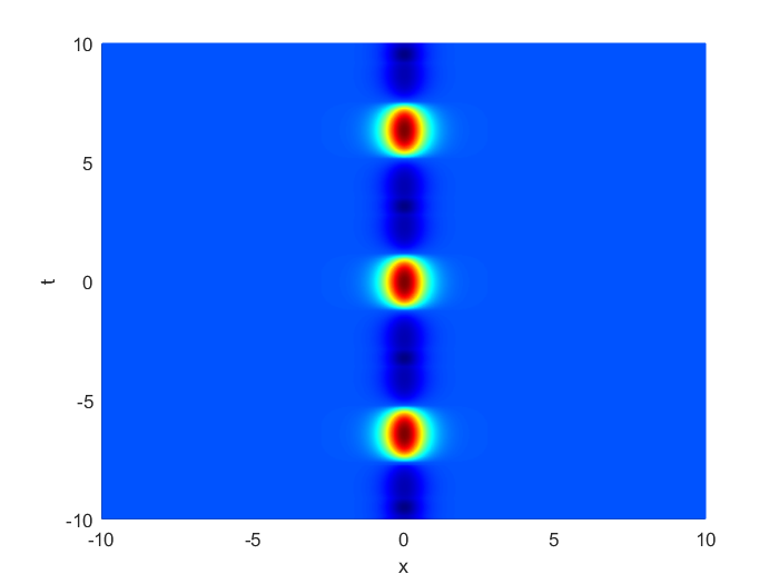
(a)(b)

Figure 2: (a) and (b) show part of the breather solution for p=3 and q=4.

Theorem 4.2.

Suppose that $\rho(x),\mu(x),v_{p}(x),v_{q}(x):\mathbb{R}^{3}\rightarrow(0,\infty)$ are radially symmetric $C^{2}$-functions such that $(H1)-(H4)$ hold and $T=2\pi\sqrt{\frac{\rho(0)}{\mu(0)}}$. Then there exists a continuum of $T$-periodic $C^{3}$-valued monochromatic breather solutions $\mathbf{u}(x,t)=e^{i\frac{2\pi}{T}t}\mathbf{u}(x)$ of (1.1), with the property $\sup_{\mathbb{R}^{3}}|\mathbf{u}(x)|e^{\gamma|x|}<\infty$.

Proof.

We use the ansatz $\mathbf{u}(x,t)=y(|x|)e^{i\frac{2\pi}{T}t}\frac{x}{|x|}$ and insert it into (1.1), then it represents a $T$-periodic breather if $y:[0,\infty)\rightarrow\mathbb{R}$ is a $C^{2}$-solution of

$$-\left(\frac{2\pi}{T}\right)^{2}\tilde{\rho}(r)+\tilde{\mu}(r)+\tilde{v}_{p}(r)|y(r)|^{p-1}+\tilde{v}_{q}(r)|y(r)|^{q-1}=0,$$ (4.6)

satisfying $y(0)=y^{\prime\prime}(0)=0$ and is exponentially decays to zero at $\infty$. Note that (4.6) can be rewritten as

$$\left(\frac{\tilde{\mu}(r)}{\tilde{v}_{q}(r)}\right)^{\frac{q-p}{q-1}}|y(r)|^{p-1}+|y(r)|^{q-1}=\left((\frac{2\pi}{T})^{2}\frac{\tilde{\rho}(r)}{\tilde{\mu}(r)}-1\right)\frac{\tilde{\mu}(r)}{\tilde{v}_{q}(r)},$$

where $\tilde{v}_{q}(r)=\left(\frac{\tilde{\mu}(r)^{p-q}}{\tilde{v}_{p}(r)^{1-q}}\right)^{\frac{1}{p-1}}$ from (4.2). We define $l:[0,\infty)\rightarrow\mathbb{R}$ with

$$l(|y(r)|)=\left(\frac{\tilde{\mu}(r)}{\tilde{v}_{q}(r)}\right)^{\frac{q-p}{q-1}}|y(r)|^{p-1}+|y(r)|^{q-1},$$

then we have

$$l^{\prime}(|y(r)|)=(p-1)\left(\frac{\tilde{\mu}(r)}{\tilde{v}_{q}(r)}\right)^{\frac{q-p}{q-1}}|y(r)|^{p-2}+(q-1)|y(r)|^{q-2}>0$$

for $1<p<q$. Thus we obtain that $l$ has an inverse $l^{-1}$, which implies that $y$ can be rewritten as

$$y(r)=\pm l^{-1}\left[\left((\frac{2\pi}{T})^{2}\frac{\tilde{\rho}(r)}{\tilde{\mu}(r)}-1\right)\frac{\tilde{\mu}(r)}{\tilde{v}_{q}(r)}\right].$$

The assumption $(H1)$ guarantees that $y$ is well-defined. By $(H3)$ and $(H4)$, it is exponentially decaying as $r\rightarrow\infty$ and by $(H2)$ we have $y(0)=y^{\prime\prime}(0)=0$, so that $\mathbf{u}(x,t)$ is a classical solution of (1.1) on $\mathbb{R}^{3}\times\mathbb{R}$. The proof of this theorem is completed. ∎

5 Conclusions and discussions

In this work, a (3+1)-dimensional radially symmetric curl-cur wave equation with double power nonlinearity is investigated. In view of the radially symmetric assumptions on the coefficients, the time periodic and spatially localized real-valued solutions of equation (1.1) are constructed. Thus, the (3+1)-dimensional wave equation reduces to a family of ordinary differential equations. By means of the ODEs technique, we prove the existence and extra exponential decay properties of real-valued breather solution of equation (1.1). Furthermore, we show that the solution can generate a continuum of phase-shifted breathers. In addition, we also construct $T$-periodic $C^{3}$-valued monochromatic breather solutions of the type $\mathbf{u}(x,t)=e^{i\frac{2\pi}{T}t}\mathbf{u}(x)$ of equation (1.1). We give an example for special coefficient functions which satisfy the assumptions of the main theorem, then exhibit the profiles of the breather solution. Our results may be a preliminary attempt in revealing optical breathers of nonlinear Maxwell’s equations in anisotropic materials. We hope that our results can help enrich the dynamic behavior of the breathers under the context of the curl-curl nonlinear wave equations.

Data Availability This work does not have any experimental data.

Conflict of interest We have no competing interests.

Acknowledgments The authors sincerely thank Professor C.E. Wayne (Boston University) for his guidance to consider the problem of breather solutions for nonlinear wave equation, and also thank the editors for very careful reading and providing many valuable comments and suggestions which led to much improvement in earlier version of this paper. This work is partially supported by NSFC Grants (12225103, 12071065 and 11871140) and the National Key Research and Development Program of China (2020YFA0713602 and 2020YFC1808301).

References

References

- [1] M.J. Ablowitz, D.J. Kaup, A.C. Newell and H. Segur, Method for solving the sine-Gordon equation, Phys. Rev. Lett. 30 (1973) 1262-1264.
- [2] G.T. Adamashvili and D.J. Kaup, Optical breathers in nonlinear anisotropic and dispersive media, Phys. Rev. E. 73 (2006), no. 6, 066613.
- [3] S. Alama and Y. Li, Existence of solutions for semilinear elliptic equations with indefinite linear part, J. Differential Equations, 96 (1992) 89-115.
- [4] A. Azzollini, V. Benci, T. D’Aprile and D. Fortunato, Existence of static solutions of the semilinear Maxwell equations, Ric. Mat. 55 (2006) 283-297.
- [5] D. Bambusi and T. Penati, Continuous approximation of breathers in one- and two-dimensional DNLS lattices, Nonlinearity 23 (2010) 143-157.
- [6] T. Bartsch, T. Dohnal, M. Plum and W. Reichel, Ground states of a nonlinear curl-curl problem in cylindrically symmetric media, NoDEA Nonlinear Diff. Equ. Appl. 23 (2016), no. 5, Art. 52, 34 pp.
- [7] B. Birnir, H.P. McKean and A. Weinstein, The rigidity of sine-Gordon breathers, Comm. Pure Appl. Math. 47 (1994) 1043-1051.
- [8] C. Blank, M. Chirilus-Bruckner, V. Lescarret and G. Schneider, Breather solutions in periodic media, Comm. Math. Phys. 302 (2011) 815-841.
- [9] K. Busch, G. von Freyman, S. Linden, S.F. Mingaleev, L. Theshelashvili and M. Wegener, Periodic nanostructures for photonics, Phys. Rep. 444 (2007) 101-202.
- [10] M. Chirilus-Bruckner and C.E. Wayne, Inverse spectral theory for uniformly open gaps in a weighted Sturm CLiouville problem, J. Math. Anal. Appl. 427 (2015) 1168-1189.
- [11] J. Denzler, Nonpersistence of breather families for the perturbed sine Gordon equation, Commun. Math. Phys. 158 (1993) 397-430.
- [12] M. Haragus and D.E. Pelinovsky, Linear instability of breathers for the focusing nonlinear Schrödinger equation, J. Nonlinear Sci. 32 (2022), no. 5, Paper No. 66, 40 pp.
- [13] A. Hirsch and W. Reichel, Real-valued, time-periodic localized weak solutions for a semilinear wave equation with periodic potentials, Nonlinearity 32 (2019) 1408-1439.
- [14] G. James, B. Sánchez-Rey and J. Cuevas, Breathers in inhomogeneous nonlinear lattices: an analysis via center manifold reduction, Rev. Math. Phys. 21 (2009) 1-59.
- [15] N.I. Karachalios, B. Sánchez-Rey, P.G. Kevrekidis and J. Cuevas, Breathers for the discrete nonlinear schrödinger equation with nonlinear hopping, J. Nonlinear Sci. 23 (2013) 205-239.
- [16] R.S. MacKay and S. Aubry, Proof of existence of breathers for time-reversible or Hamiltonian networks of weakly coupled oscillators, Nonlinearity 7 (1994) 1623-1643.
- [17] R. Mandel and D. Scheider, Variational methods for breather solutions of nonlinear wave equations, Nonlinearity 34 (2021) 3618-3640.
- [18] J. Mederski, Ground states of time-harmonic semilinear Maxwell equations in with vanishing permittivity, Arch. Ration. Mech. Anal. 218 (2015) 825-861.
- [19] J. Mederski, The Brezis-Nirenberg problem for the curl-curl operator, J. Funct. Anal. 274 (2018) 1345-1380.
- [20] A. Pankov, Periodic nonlinear Schrödinger equation with application to photonic crystals, Milan J. Math. 73 (2005) 259-287.
- [21] A. Pankov, Gap solitons in periodic discrete nonlinear Schrödinger equations, Nonlinearity 19 (2006) 27-40.
- [22] D.E. Pelinovsky, G. Simpson and M.I. Weinstein, Polychromatic solitary waves in a periodic and nonlinear Maxwell system, SIAM J. Appl. Dyn. Syst. 11 (2012) 478-506.
- [23] M. Plum and W. Reichel, A breather construction for a semilinear curl-curl wave equation with radially symmetric coefficients, J. Elliptic Parabol. Equ. 2 (2016) 371-387.
- [24] B.E.A. Saleh and M.C. Teich, Fundamentals of Photonics, 2nd edn. Wiley, New York 2007.
- [25] D. Scheider, Breather solutions of the cubic Klein-Gordon equation, Nonlinearity 33 (2020) 7140-7166.
- [26] H. Shi and Y. Zhang, Existence results of solitons in discrete non-linear Schrödinger equations, European J. Appl. Math. 27 (2016) 726-737.
- [27] W.R. Smith and J.A.D. Wattis, Necessary conditions for breathers on continuous media to approximate breathers on discrete lattices, European J. Appl. Math. 27 (2016) 23-41.
- [28] W.A. Strauss, Existence of solitary waves in higher dimensions, Comm. Math. Phys. 55 (1977) 149-162.
- [29] C.A. Stuart, Self-trapping of an electromagnetic field and bifurcation from the essential spectrum, Arch. Rational Mech. Anal. 113 (1990) 65-96.