Partial Network Cloning

Abstract

In this paper, we study a novel task that enables partial knowledge transfer from pre-trained models, which we term as Partial Network Cloning (PNC). Unlike prior methods that update all or at least part of the parameters in the target network throughout the knowledge transfer process, PNC conducts partial parametric “cloning” from a source network and then injects the cloned module to the target, without modifying its parameters. Thanks to the transferred module, the target network is expected to gain additional functionality, such as inference on new classes; whenever needed, the cloned module can be readily removed from the target, with its original parameters and competence kept intact. Specifically, we introduce an innovative learning scheme that allows us to identify simultaneously the component to be cloned from the source and the position to be inserted within the target network, so as to ensure the optimal performance. Experimental results on several datasets demonstrate that, our method yields a significant improvement of $\>5\%$ in accuracy and 50% in locality when compared with parameter-tuning based methods. Our code is available at https://github.com/JngwenYe/PNCloning.

1 Introduction

With the recent advances in deep learning, an increasingly number of pre-trained models have been released online, demonstrating favourable performances on various computer vision applications. As such, many model-reuse approaches have been proposed to take advantage of the pre-trained models. In practical scenarios, users may request to aggregate partial functionalities from multiple pre-trained networks, and customize a target network whose competence differs from any network in the model zoo.

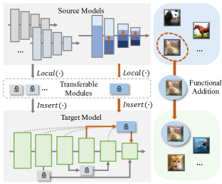
Figure 1: Illustration of partial network cloning. Given a set of pre-trained source models, we “clone” the transferable modules from the source, and insert them into the target model (left) while preserving the functionality (right).

A straightforward solution to the functionality dynamic changing is to re-train the target network using the original training dataset, or to conduct finetuning together with regularization strategies to alleviate catastrophic forgetting [19, 3, 39], which is known as continual learning. However, direct re-training is extremely inefficient, let alone the fact that original training dataset is often unavailable. Continual learning, on the other hand, is prone to catastrophic forgetting especially when the amount of data for finetuning is small, which, unfortunately, often occurs in practice. Moreover, both strategies inevitably overwrite the original parameters of the target network, indicating that, without explicitly storing original parameters of the target network, there is no way to recover its original performance or competence when this becomes necessary.

In this paper, we investigate a novel task, termed as Partial Network Cloning (PNC), to migrate knowledge from the source network, in the form of a transferable module, to the target one. Unlike prior methods that rely on updating parameters of the target network, PNC attempts to clone partial parameters from the source network and then directly inject the cloned module into the target, as shown in Fig. 1. In other words, the cloned module is transferred to the target in a copy-and-paste manner. Meanwhile, the original parameters of the target network remain intact, indicating that whenever necessary, the newly added module can be readily removed to fully recover its original functionality. Notably, the cloned module per se is a fraction of the source network, and therefore requirements no additional storage expect for the lightweight adapters. Such flexibility to expand the network functionality and to detach the cloned module without altering the base of the target or allocating extra storage, in turn, greatly enhances the utility of pre-trained model zoo and largely enables plug-and-play model reassembly.

Admittedly, the ambitious goal of PNC comes with significant challenges, mainly attributed to the black-box nature of the neural networks, alongside our intention to preserve the performances on both the previous and newly-added tasks of the target. The first challenge concerns the localization of the to-be-cloned module within the source network, since we seek discriminant representations and good transferability to the downstream target task. The second challenge, on the other hand, lies in how to inject the cloned module to ensure the performance.

To solve these challenges, we introduce an innovative strategy for PNC, through learning the localization and insertion in an intertwined manner between the source and target network. Specifically, to localize the transferable module in the source network, we adopt a local-performance-based pruning scheme for parameter selection. To adaptively insert the module into the target network, we utilize a positional search method in the aim to achieve the optimal performance, which, in turn, optimizes the localization operation. The proposed PNC scheme achieves performances significantly superior to those of the continual learning setting ($5\%\sim 10\%$), while reducing data dependency to $30\%$.

Our contributions are therefore summarized as follows.

• We introduce a novel yet practical model re-use setup, termed as partial network cloning (PNC). In contrast to conventional settings the rely on updating all or part of the parameters in the target network, PNC migrates parameters from the source in a copy-and-paste manner to the target, while preserving original parameters of the target unchanged.

• We propose an effective scheme towards solving PNC, which conducts learnable localization and insertion of the transferable module jointly between the source and target network. The two operations reinforce each other and together ensure the performance of the target network.

• We conduct experiments on four widely-used datasets and showcase that the proposed method consistently achieves results superior to the conventional knowledge-transfer settings, including continual learning and model ensemble.

2 Related Work

2.1 Life-long Learning

Life-long/online/incremental learning, which is capable of learning, retaining and transferring knowledge over a lifetime, has been a long-standing research area in many fields [43, 35, 51, 52]. The key of continual learning is to solve catastrophic forgetting, and there are three main solutions, which are the regularization-based methods [19, 3, 39, 20], the rehearsal-based methods [4, 34, 40] and architecture-based methods [24, 18, 45, 16].

Among these three streams of methods, the most related one to PNC is the architecture-based pruning, which aims at minimizing the inter-task interference via newly designed architectural components. Li et al. [18] propose to separate the explicit neural structure learning and the parameter estimation, and apply evolving neural structures to alleviate catastrophic forgetting. At each incremental step, DER [45] freezes the previously learned representation and augment it with additional feature dimensions from a new learnable feature extractor. Singh et al. [36] choose to calibrate the activation maps produced by each network layer using spatial and channel-wise calibration modules and train only these calibration parameters for each new task.

The above incremental methods are fine-tuning all or part of the current network to solve functionality changes. Differently, we propose a more practical life-long solution, which learns to transfer the functionality from pre-trained networks instead of learning from the new coming data.

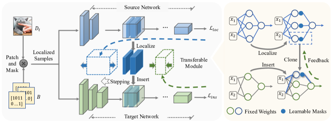
Figure 2: The proposed partial network cloning framework. The localized samples are fed into the source network for the original transferable module localization. To refine the transferable module, we learn how to locate and insert it, with the network weights fixed.

2.2 Network Editing

Model editing is proposed to fix the bugs in networks, which aims to enable fast, data-efficient updates to a pre-trained base model’s behavior for only a small region of the domain, without damaging model performance on other inputs of interest [37, 26, 38].

A popular approach to model editing is to establish learnable model editors, which are trained to predict updates to the weights of the base model to produce the desired change in behavior [37]. MEND [25] utilizes a collection of small auxiliary editing networks as a model editor. Eric et al. [26] propose to store edits in an explicit memory and learn to reason over them to modulate the base model’s predictions as needed. Provable point repair algorithm [38] finds a provably minimal repair satisfying the safety specification over a finite set of points. Cao et al. [5] propose to train a hyper-network with constrained optimization to modify without affecting the rest of the knowledge, which is then used to predict the weight update at test time.

Different from network edition that directly modifies a certain of weights to fix several bugs, our work do the functionality-wise modification by directly inserting the transferable modules.

2.3 Model Reuse

With a bulk of pre-trained models online, model reuse becomes a hot topic, which attempts to construct the model by utilizing existing available models, rather than building a model from scratch. Model reuse is applied for the purpose of reducing the time complexity, data dependency or and expertise requirement, which is studied by knowledge transfer [8, 6, 7, 55, 53, 30] and model ensemble [27, 33, 1, 41].

Knowledge transfer [31, 21, 46, 47, 50, 49, 22] utilizes the pre-trained models by transferring knowledge from these networks to improve the current network, which has promoted the performance of domain adaptation [12], multi-task learning [42], Few-Shot Learning [17] and so on [13]. For example, KTN [28] is proposed to jointly incorporate visual feature learning, knowledge inferring and classifier learning into one unified framework for their optimal compatibility. To enable transferring knowledge from multiple models, Liu et al.  [23] propose an adaptive multi-teacher multi-level knowledge distillation learning framework which associates each teacher with a latent representation to adaptively learn the importance weights.

Model ensemble [14, 15, 48] integrates multiple pre-trained models to obtain a low-variance and generalizable model. Peng et al. [27] apply sample-specific ensemble of source models by adjusting the contribution of each source model for each target sample. MEAL [33] proposes an adversarial-based learning strategy in block-wise training to distill diverse knowledge from different trained models.

The above model reuse methods transfer knowledge from networks to networks, with the base functionality unchanged. We make the first step work to directly transfer part of the knowledge into a transferable module by cloning part of the parameters from the source network, which enables network functionality addition.

3 Proposed Method

The goal of the proposed partial network cloning framework is to clone part of the source networks to the target network so as to enable the corresponding functionality transfer in the target network.

The illustration of the proposed PNC framework is shown in Fig. 2, where we extract a transferable module that could be directly inserted into the target network.

3.1 Preliminaries

Given a total number of $P$ pre-trained source models $\mathcal{M}_{s}=\{\mathcal{M}_{s}^{0},\mathcal{M}_{s}^{1},...,\mathcal{M}_{s}^{P-1}\}$, each $\mathcal{M}_{s}^{\rho}$ ($0\leq\rho<P$) serves for cloning the functionality $t_{s}^{\rho}$, where $t_{s}^{\rho}$ is a subset of the whole functionality set of $\mathcal{M}_{s}^{\rho}$ and the to-be-cloned target set is denoted as $T_{s}=\{t_{s}^{0},t_{s}^{1},...,t_{s}^{P-1}\}$. The partial network cloning is applied on the target model $\mathcal{M}_{t}$ for new functionalities addition, which is the pre-trained model on the original set $T_{t}$ ($T_{t}\cap T_{s}=\emptyset$).

Partial network cloning aims at expending the functionality set of target network on the new $T_{s}$ by directly cloning. In the proposed framework, it is achieved by firstly extracting part of $\mathcal{M}_{s}$ to form a transferable module $\mathcal{M}_{f}$, and then inserting it into target model $\mathcal{M}_{t}$ to build a after-cloned target network $\mathcal{M}_{c}$. The whole process won’t change any weights of the source and target models, and also each transferable module is directly extracted from the source model free of any tuning on its weights. Thus, the process can be formulated as:

$$\begin{split}\mathcal{M}_{c}\leftarrow Clone(\mathcal{M}_{t},M,\mathcal{M}_{s},R),\end{split}$$ (1)

which is directly controlled by $M$ and $R$, where $M$ is a set of selection functions for deciding how to extract the explicit transferable module on source networks $\mathcal{M}_{s}$, and $R$ is the position parameters for deciding where to insert the transferable modules to the target network. Thus, partial network cloning $Clone(\cdot)$ consists of two steps:

$$\begin{split}\mathcal{M}_{f}^{\rho}&\leftarrow Local(\mathcal{M}_{s}^{\rho},M^{\rho}),\\ \mathcal{M}_{c}&\leftarrow Insert_{\rho=0}^{P}(\mathcal{M}_{t},\mathcal{M}_{f}^{\rho},R^{\rho}),\end{split}$$ (2)

where both $M$ and $R$ are learnable and optimized jointly. Once $M$ and $R$ are learned, $\mathcal{M}_{c}$ can be determined with some lightweight adapters.

Notably, we assume that only the samples related to the to-be-cloned task set $T_{s}$ are available in the whole process, keeping the same setting of continual learning. And to be practically feasible, partial network cloning must meet three natural requirements:

• Transferability: The extracted transferable module should contain the explicit knowledge of the to-be-cloned task $T_{s}$, which could be transferred effectively to the downstream networks;

• Locality: The influence on the cloned model $\mathcal{M}_{c}$ out of the target data $D_{t}$ should be minimized;

• Efficiency: Functional cloning should be efficient in terms of runtime and memory;

• Sustainability: The process of cloning wouldn’t do harm to the model zoo, meaning that no modification the pre-trained models are allowed and the cloned model could be fully recovered.

In what follows, we consider the partial network cloning from one pre-trained network to another, which could certainly be extended to the multi-source cloning cases, thus we omit $\rho$ in the rest of the paper.

3.2 Localize with pruning

Localizing the transferable module from the source network is actually to learn the selection function $M$.

In order to get an initial transferable module $\mathcal{M}_{f}$, we locate the explicit part in the source network $\mathcal{M}_{s}$ that contributes most to the final prediction. Thus, the selection function $M$ is optimized by the transferable module’s performance locally on the to-be-cloned task $T_{s}$.

Here, we choose the selection function as a kind of mask-based pruning method mainly for two purposes: the first one is that it applies the binary masks on the filters for pruning without modifying the weights of $\mathcal{M}_{s}$, thus, ensuring sustainability; the other is for transferability that pruning would be better described as ‘selective knowledge damage’ [9], which helps for partial knowledge extraction.

Note that unlike the previous pruning method with the objective function to minimize the error function on the whole task set of $\mathcal{M}_{s}$, here, the objective function is designed to minimize the locality performance on the to-be-cloned task set $T_{s}$. Specifically, for the source network $\mathcal{M}_{s}$ with $L$ layers $W_{s}=\{w_{s}^{0},w_{s}^{1},...,w_{s}^{L-1}\}$, the localization can be denoted as:

$$\begin{split}\mathcal{M}_{f}=&M\cdot\mathcal{M}_{s}\Leftrightarrow\{m^{l}\cdot w_{s}^{l}|0\leq l<L\},\\ M=&\arg\max_{M}\ Sim(\mathcal{M}_{f},\mathcal{M}_{s}|D_{t})\\ &-Sim(\mathcal{M}_{f},\mathcal{M}_{s}|\overline{D}_{t}),\end{split}$$ (3)

where $M=\{m^{0},m^{1},...,m^{L-1}\}$ is a set of learnable masking parameters, which are also the selection function as mentioned in Eq. 1. $Sim(\cdot|\cdot)$ represents the conditional similarity among networks, $\overline{D}_{t}$ is the rest data set of the source network. The localization to extract the explicit part on the target $D_{t}$ is learned by maximizing the similarity between $\mathcal{M}_{s}$ and $\mathcal{M}_{f}$ on $D_{t}$ while minimizing it on $\overline{D}_{t}$.

Considering the black-box nature of deep networks that all the knowledge (both from $D_{t}$ and $\overline{D}_{t}$) is deeply and jointly embedded in $\mathcal{M}_{s}$, it is non-trivial to calculate the similarity on the ${D_{t}}$-neighbor source network $\mathcal{M}_{s}|_{D_{t}}$. Motivated by LIME [32] that utilizes interpretable representations locally faithful to the classifier, we train a model set containing $N$ small local models $\mathcal{G}=\{g_{i}\}^{(N)}$ to model the source $\mathcal{M}_{s}$ in the $D_{t}$ neighborhood, and then use the local model set as the surrogate: $\mathcal{G}\approx\mathcal{M}_{s}|_{D_{t}}$. To obtain $\mathcal{G}$, for each $x_{i}\in D_{t}$, we get its augmented neighborhood by separating it into patches (i.e. $8\times 8$) and applying the patch-wise perturbations with a set of binary masks $B$. Thus, $\mathcal{G}$ is obtained by:

$$\min_{g_{i}}\frac{1}{|B|}\sum_{b\in B}\Pi_{b}\cdot\big{\|}\mathcal{M}_{s}(b\cdot x_{i})-g_{i}(b))\big{\|}^{2}+\Omega(g_{i}),$$ (4)

where $\Pi_{b}$ is the weight measuring sample locality according to ${x}_{i}$, $\Omega(g_{i})$ is the complexity of $g_{i}$ and $|B|$ donates the total number of masks. $\mathcal{G}$ is optimized by the least square method and more details are given in the supplementary. For each $x_{i}$, we calculate a corresponding $g_{i}$. And actually, we set $N<|D_{t}|$ (about $30\%$), which is clarified in the experiments.

The new $\mathcal{G}$, calculated from the original source network $\mathcal{M}_{s}$ in the $D_{t}$ neighborhood, models the locality of the target task $T_{s}$ on $\mathcal{M}_{s}$. Note that $\mathcal{G}$ can be calculated in advance for each pre-trained model, as it could also be a useful tool for the model distance measurement and others [10]. In this paper, $\mathcal{G}$ perfectly matches our demand for the transferable module localization. So the localization process in Eq. 3 could be optimized as:

$$\begin{split}\min_{M}\sum_{g_{i}\in\mathcal{G}}\sum_{b\in B}\Big{\|}&f_{t}[\mathcal{M}_{s}\big{(}M\cdot W_{s};b\cdot x\big{)}]-f_{t}[g_{i}(b)]\Big{\|}^{2}\\ &s.t.\quad|m^{l}|\leq c^{l}\end{split}$$ (5)

where $f_{t}$ is for selecting the $T_{s}$ related output and $c^{l}$ is the parameter controlling the number of non-zero values of $M$ ($c^{l}<|W^{l}|$). And for inference, the learned soft masks $M$ are binarized by selecting $c^{l}$ filters with the top-$c^{l}$ masking values in each layer.

3.3 Insert with adaptation

After the transferable module $\mathcal{M}_{f}$ being located at the source network, it could be directly extracted from $\mathcal{M}_{s}$ with $M$, without any modifications on its weights. Then the following step is to decide where to insert $\mathcal{M}_{f}$ into $\mathcal{M}_{t}$, as to get best insertion performance.

The insertion is controlled by the position parameter $R$ mentioned in Eq. 3. Following most of the model reuse settings that keep the first few layers of the pre-trained model as a general feature extractor, the learning-to-insert process with $R$ is simplified as finding the best position ($R$-th layer to insert $\mathcal{M}_{f}$). The insertion could be denoted as:

$$\begin{split}\mathcal{M}_{c}^{R}=&\mathcal{M}_{t}\big{(}W_{t}^{[0:R]}\big{)}\circ\big{\{}\mathcal{M}_{t}\big{(}W_{t}^{[R:L]}\big{)},\mathcal{M}_{f}\big{\}},\\ R^{*}=&\arg\max_{R}\ Sim(\mathcal{M}_{f},\mathcal{M}_{c}^{R}|D_{t})\\ &+Sim(\mathcal{M}_{t},\mathcal{M}_{c}^{R}|D_{o}),\end{split}$$ (6)

where $D_{o}$ is the original set for pre-training the target network, and $D_{o}\cup D_{t}=\emptyset$. The cloned $\mathcal{M}_{c}$ is obtained by the parallel connection of the transferable module into the target network $\mathcal{M}_{t}$. Thus the insertion learned by Eq. 6 is to find the best insertion position by maximizing the similarity between $\mathcal{M}_{f}$ and $\mathcal{M}_{c}$ on $D_{t}$ (for the best insertion performance on $D_{t}$) and the similarity between $\mathcal{M}_{t}$ and $\mathcal{M}_{c}$ on $D_{o}$ (for the least accuracy drop on the previously learned $D_{o}$).

In order to learn the best position R, we need maximize the network similarities $Sim(|)$. Different from the solution used to optimize the objective function while localizing, insertion focuses on the prediction accuracies on the original and the to-be-cloned task set. So we use the network outputs to calculate $Sim(\cdot)$, which is the KL-divergence loss $\mathcal{L}_{kd}$. we write:

$$\begin{split}\min_{\mathcal{F}_{c},\mathcal{A}}&\mathcal{L}_{kd}\circ f_{t}\big{[}\mathcal{F}_{c}(\mathcal{A};\mathcal{M}_{c}^{R}(B\cdot x)),\mathcal{G}(B)\big{]}\\ +&\mathcal{L}_{kd}\circ\overline{f}_{t}\big{[}\mathcal{F}_{c}(\mathcal{A};\mathcal{M}_{c}^{R}(B\cdot x)),\mathcal{M}_{t}(B\cdot x)\big{]},\\ &s.t.\quad R\in\{0,1,...,L-1\}\end{split}$$ (7)

where $f_{t}$ is for selecting the $T_{s}$ related output while $\overline{f}_{t}$ is for selecting the rest. $\mathcal{F}_{c}$ is the extended fully connection layers from the original FC layers of $\mathcal{M}_{t}$. And we add an extra adapter module $\mathcal{A}$ to do the feature alignment for the transferable module, which further enables cloning between heterogeneous models. The adapter is consisted of one $1\times 1$ conv layer following with ReLu, which, comparing with $\mathcal{M}_{s}$ and $\mathcal{M}_{t}$, is much smaller in scale. $\mathcal{G}$ and $B$ are defined in Eq. 5.

While training, $R$ is firstly set to be $L-1$ and then moving layer by layer to $R=0$. In each moving step, we fine-tune the adapter $\mathcal{A}$ and the corresponding fully connected layers $\mathcal{F}_{c}$. It is a light searching process, since only a few of weights ($\mathcal{A}$ and $\mathcal{F}_{c}$) need to be fine-tuned for only a couple epochs (5$\sim$ 20). Extra details for heterogeneous model pair are in the supplementary. Please note that although applying partial network cloning from the source to the target needs two steps ($Clone(\cdot)$ and $Insert(\cdot)$), the learning process is not separable and are interacted on each other. As a result, the whole process can be jointly formulated as:

$$\begin{split}\!\min_{M,\mathcal{F}_{c},\mathcal{A}}\mathcal{L}_{loc}\Big{(}\mathcal{M}_{s}^{[0:R]}&,M\!\cdot\!W_{s}^{[R:L]},\mathcal{G}\Big{)}\!+\!\mathcal{L}_{ins}\Big{(}\mathcal{M}_{t}^{[0:R]},\\ \mathcal{A}\circ(M&\!\cdot\!W_{s}^{[R:L]}),\mathcal{M}_{t}^{[R:L]},\mathcal{F}_{c},\mathcal{G}\Big{)},\\ where&\quad R:(L-1)\rightarrow 0\end{split}$$ (8)

where $\mathcal{L}_{loc}(\cdot)$ is the objective function in Eq. 5 and $\mathcal{L}_{ins}(\cdot)$ is the objective function in Eq. 7. And in this objective function, $\mathcal{M}_{s}$ and $\mathcal{M}_{t}$ are using the same $R$ for simplification, while in practice a certain ratio exists for the heterogeneous model pair.

Once the above training process is completed, we could roughly estimate the performance by the loss convergence value, which follows the previous work [54]. Finally the layer with least convergence value is marked as the final $R$. The insertion is completed by this determined $R$ and the corresponding $\mathcal{A}$ and $\mathcal{F}_{c}$.

3.4 Cloning in various usages

The proposed partial network cloning by directly inserting a fraction of the source network enables flexible reuse of the pre-trained models in various practical scenarios.
Scenario I: Partial network cloning is a better form for information transmission. When there is a request for transferring the networks, it is better to transfer the cloned network obtained by PNC as to reduce latency and transmission loss.

In the transmission process, we only need to transfer the set $\{M,R,\mathcal{A},\mathcal{F}_{c}\}$, which together with the public model zoo, could be recovered by the receiver. $\{M,R,\mathcal{A},\mathcal{F}_{c}\}$ is extremely small in scale comparing with a complete network, thus could reduce the transmission latency. And if there is still some transmission loss on $\mathcal{A}$ and $\mathcal{F}_{c}$, it could be easily revised by the receiver by fine-tuning on $D_{t}$. As a result, PNC provides a new form of networks for high-efficiency transmission.
Scenario II: Partial network cloning enables model zoo online usage. In some resource limited situation, the users could flexibly utilize model zoo online without downloading it on local.

Note that the cloned model is determined by $Clone(\mathcal{M}_{t},M,\mathcal{M}_{s},R)$, $\mathcal{M}_{t}$ and $\mathcal{M}_{s}$ are fixed and unchanged in the whole process. There is not any modifications on the pre-trained models ($\mathcal{M}_{t}$ and $\mathcal{M}_{s}$) nor introducing any new models. PNC enables any functional combinations in the model zoo, which also helps maintain a good ecological environment for the model zoo, since PNC with $M$ and $R$ is a simple masking and positioning operation, which is easy of revocation. Thus, the proposed PNC supports to establish a sustainable model zoo online inference platform.

4 Experiments

We provide the experimental results on four publicly available benchmark datasets, and evaluate the cloning performance in the commonly used metrics as well as the locality metrics. And we compare the proposed method with the most related field – continual learning, to show concrete difference between these two streams of researches. More details and experimental results including partially cloning from multiple source networks, can be found in the supplementary.

4.1 Experimental settings

Datasets. Following the setting of previous continual methods, we report experiments on MNIST, CIFAR-10, CIFAR-100 and TinyImageNet datasets. For MNIST, CIFAR-10 and CIFAR-100 datasets, we are using input size of $32\times 32$. For TinyImageNet dataset, we are using input size of $256\times 256$. In the normal network partial cloning setting, the first 50% of classes are selected to pre-train the target network $\mathcal{M}_{t}$, and the last 50% of classes classes are selected to pre-train the source network $\mathcal{M}_{s}$.

In the partial network cloning process, $30\%$ of the training data are used for each sub dataset, which reduces the data dependency to 30%. And for training the local model set $\mathcal{G}$, we set $|B|=100$ and segment the input into $4\times 4$ patches for the MNIST, CIFAR-10 and CIFAR-100 datasets, set $|B|=1000$ and segment the input into $8\times 8$ patches for the Tiny-ImageNet dataset.

Training Details. We used PyTorch framework for the implementation. We apply the experiments on the several network backbones, including plain CNN, LeNet, ResNet, MobileNetV2 and ShuffleNetV2. In the pre-training process, we employ a standard data augmentation strategy: random crop, horizontal flip, and rotation. In the process of partial cloning, 10 epochs fine-tuning are operated for each step on MNIST and CIFAR-10 datasets, 20 epochs for CIFAR-100 and Tiny-ImageNet datasets.

For simplifying and accelerating the searching process in Eq. 8, we split LeNet into 3 blocks, the ResNet-based network into 5 blocks, MobileNetV2 into 8 blocks and ShuffleNetV2 into 5 blocks (excluding the final FC layers). Thus the block-wise adjustment for $R$ is applied for acceleration.

Evaluation Metrics. For the cloning performance evaluation, we evaluate the task performance by average accuracy:‘Ori. Acc’ (accuracy on the original set), ‘Tar. Acc’ (accuracy on the to-be-cloned set) and ‘Avg. Acc’ (accuracy on the original and to-be-cloned set), which is evaluated on the after-cloning target network $\mathcal{M}_{c}$.

For evaluating the transferable module quality evaluation on local-functional representative ability, we use the conditional similarity $Sim(|)$ with $\mathcal{G}$ [11], which can be calculated as:

$$Sim(\mathcal{M}_{a}|D_{a},\mathcal{M}_{b}|D_{b})=Sim_{cos}\theta(\mathcal{G}_{a},\mathcal{G}_{b})$$ (9)

where $Sim_{cos}(\cdot)$ is the cosine similarity, $\mathcal{G}_{a}$ and $\mathcal{G}_{b}$ are the corresponding local model sets of $\mathcal{M}_{a}(D_{a})$ and $\mathcal{M}_{b}(D_{b})$.

For evaluating the transferable module quality on transferability to other networks other than the target network, it is in the supplementary.

4.2 Experimental Results

Table 1: Overall performance on partial network cloning on MNIST, CIFAR10, CIFAR100 and Tiny-ImageNet datasets. We report the accuracies to evaluate the performance, including the comparison with the other functional addition methods and the ablation study. We choose ‘Continual+KD’ as baseline and mark the accuracy promotion in blue, accuracy drop in red.

	Acc on MNIST (LeNet5, #3 Steps)						Acc on CIFAR-10 (ResNet-18, #5 Steps)
Method	Ori.-S	Tar.-S	Avg.-S	Ori.-M	Tar.-M	Avg.-M	Ori.-S	Tar.-S	Avg.-S	Ori.-M	Tar.-M	Avg.-M
Pre-trained	99.7	99.5	99.7	99.7	99.5	99.6	95.9	97.2	96.1	95.9	97.6	96.5
Joint+Full Set	99.8	98.3	99.6	99.7	99.3	99.5	95.2	96.8	95.5	94.4	95.1	94.7
Continual	83.4-10.1	100.0+17.3	86.2-5.5	65.1-27.9	98.8+16.8	77.7-11.2	67.7+2.8	97.2+2.6	75.3-14.8	92.8+18.7	78.2+16.6	87.3-2.1
Direct Ensemble	94.6+1.1	56.1-26.4	88.2-3.5	94.6+1.6	81.9-0.1	89.8+0.9	90.5+25.6	39.3-55.3	82.0+12.1	90.5+16.4	43.8-17.8	73.0+3.6
Continual+KD	93.5	82.7	91.7	93.0	82.0	88.9	64.9	94.6	69.9	74.1	61.6	69.4
PNC-F (w/o Local)	87.7-5.8	100.0+17.3	90.0-1.7	90.9-2.1	98.2+16.2	93.6+4.7	88.6+23.7	97.3+2.7	90.1+20.2	85.5+11.4	95.8+34.2	89.4+20.0
PNC-F (w/o Insert)	86.9-6.6	100.0+17.3	89.1-2.6	90.4-2.6	97.7+15.7	93.1+4.2	86.1+21.2	96.8+2.2	87.9+18.0	86.0+11.9	96.2+34.6	89.8+30.4
PNC-F (full)	88.5-5.0	99.7+17.0	90.4-2.6	91.1-1.9	98.8+16.8	94.0+5.1	83.0+18.1	96.5+1.9	85.3+15.4	85.4+11.3	95.5+33.9	89.2+19.8
PNC (w/o Local)	93.6+0.1	96.2+13.5	94.0+2.3	92.9-0.1	94.0+12.0	93.3+4.4	90.5+25.6	93.9-0.7	91.7+21.8	87.1+13.0	94.6+33.1	89.9+29.8
PNC (w/o Insert)	92.8-0.7	99.5+16.8	93.9+2.2	91.9-1.1	97.3+15.3	93.9+5.0	89.5+24.6	94.4-0.2	90.3+20.4	89.2+15.1	94.7+33.2	91.3+21.9
PNC (Ours, full)	96.4+2.9	99.7+17.0	97.0+5.3	96.2+3.2	97.815.8	96.8+7.9	94.9+30.0	95.5+0.9	95.0+25.1	93.7+19.6	94.5+32.9	94.0+24.6
	Acc on CIFAR-100 (ResNet-50, #5 Steps)						Acc on Tiny-ImageNet ( ResNet-18, #5 Steps)
Method	Ori.-S	Tar.-S	Avg.-S	Ori.-M	Tar.-M	Avg.-M	Ori.-S	Tar.-S	Avg.-S	Ori.-M	Tar.-M	Avg.-M
Pre-trained	80.0	80.3	80.1	80.0	77.2	79.0	71.3	67.6	70.7	71.3	68.9	70.4
Joint+Full Set	78.0	74.9	77.5	76.3	77.9	76.9	63.1	60.8	62.7	63.7	61.6	62.9
Direct Ensemble	59.3-6.2	46.4-26.3	57.2-9.6	56.0-18.4	46.4-26.6	52.4-21.5	58.0+0.8	35.9-20.5	54.3-2.8	50.6-9.3	30.2-27.9	43.0-16.3
Continual	52.3-13.2	79.4+6.7	56.8-9.9	58.8-15.6	78.0+5.0	66.0-7.9	54.6-2.6	70.1+13.7	57.2+0.1	55.9-4.0	64.9+6.8	59.3+0.1
Continual + KD	65.5	72.7	66.7	74.4	73.0	73.9	57.2	56.4	57.1	59.9	58.1	59.2
PNC (w/o Local)	72.2+6.7	70.4-2.3	71.9+5.2	75.7+1.3	68.3-4.7	72.9-1.0	65.6+8.4	52.5-3.9	63.4+6.4	56.4-3.5	55.9-2.2	56.2-3.0
PNC (w/o Insert)	63.2-2.3	76.1+3.4	65.4-1.3	66.1-8.3	76.0+3.0	69.8-4.1	60.7+3.5	63.5+7.1	61.2+4.1	58.8-1.1	60.9+2.8	59.6+0.4
PNC (Ours, full)	76.7+11.2	74.9+2.2	76.4+9.7	76.9+2.5	76.5+3.5	76.8+2.9	63.2+6.0	60.7+4.3	62.8+5.7	63.5+3.6	60.4+2.3	62.3+3.1

4.2.1 Overall Performance

Table 1 shows overall performance of partial network cloning on MNIST, CIFAR-10, CIFAR-100 and Tiny-ImageNet datasets, where the target network and the source network are set to be the same architecture and the number of search steps $R$ is also listed. We compare the proposed partial network cloning (‘PNC’) with the baseline ‘Pre-trained’ original networks ( Acc on $\mathcal{M}_{s}$ and $\mathcal{M}_{t}$), the ensemble network of the source and the target (‘Direct Ensemble’), the networks scratch trained on the set including the original and the target (‘Joint + Full set’), the continual-learned network with some regularization item (‘Continual’) and the continual-learned network with KD loss from the source network (‘Continual+KD’). Specially, we compare the proposed ‘PNC’ with ‘PNC-F’, where ‘PNC-F’ is the afterward all-parameter-tuned version of ‘PNC’ on the to-be-cloned dataset. And we also give the comparisons on the small-scale functionality addition (‘-S’, 20% of the source functionalities are transferred), and middle-scale functionality addition (‘-S’, 60% of the source functionalities are transferred).

From Table 1, several observations are obtained. Firstly, the proposed PNC is capable of dealing with various datasets and network architectures and its effectiveness has been proved on four datasets and on different network architectures. Secondly, the full setting PNC gives the best solution to the new functionality addition task, our full setting (‘PNC(full)’) outperforms almost all of the other methods. Thirdly, PNC shows better performance when cloning smaller functionality (‘Avg.-S’ vs ‘Avg.-M’), and it is practical in use when the most related network is chosen as the target and minor functionality is added with the proposed PNC. Finally, fully fine-tuning all the parameters of $\mathcal{M}_{c}$ after PNC doesn’t bring any benefits (‘PNC’ vs ‘PNC-F’), since fine-tuning with the to-be-cloned dataset would bring bias on the new functionality.

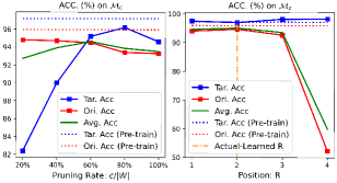
Figure 3: The performance on partial network cloning with different scales of the transferable module.

4.2.2 More Analysis of the Transferable Module

How does the scale of the transferable module influence the cloning performance? The transferable module can be denoted as $\mathcal{M}_{f}\leftarrow M\cdot W_{s}^{[R:L]}$. And the scale of the transferable module is influenced by two factors, which are the selection function $M$ and the position parameters $R$. We explore the influence of the scale on the CIFAR-10, with the same setting from Table 1 of cloning small functionality. The selection function $M$ is directly controlled by the masking rate ${c}/{|W|}$ ($0\leq l<L$, defined in Eq. 5), where larger $c^{l}$ makes larger transferable modules, shown in Fig. 3 (left). As can be observed from the figure, the accuracy of the original functionality (‘Ori. Acc’) slightly decreases with larger $\mathcal{M}_{f}$. While larger $\mathcal{M}_{f}$ doesn’t ensure higher accuracy of the to-be-cloned function (‘Tar. Acc’, first increase and then drop), indicating that the appropriate localization strategy on the source instead of inserting the whole source network benefits a lot.

The position parameter $R$ ($0\leq l<L$) is learned in the insertion process, here we show the performance for $R=1\sim 4$, which further shows the validation of our selection strategy. Bigger $R$ makes smaller transferable modules, the accuracy based on which is shown in Fig. 3 (right). The accuracy on the to-be-cloned set (‘Tar. Acc’) doesn’t largely influenced by it, while it does influence the accuracy on the original set (‘Ori. Acc’) a lot. Notably, $R=2$ is the position learned in the insertion process, which shows to the best according to the average accuracy (‘Avg. Acc’).

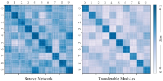
Figure 4: The similarity matrix maps computed on the source network and on the transferable modules on MNIST dataset. Deeper color indicates higher similarity.

Has the transferable module been explicitly localized? For evaluating the quality of the transferable module on whether the learned localization strategy $Local(\cdot)$ has successfully selected the explicit part for the to-be-cloned functionality or not, we compute the similarity matrix for the source network and the transferable module, which is displayed in Fig. 4. The comparison is conducted on the MNIST dataset, which is split into 10 sub-datasets ($D_{0}\sim D_{9}$, according to the label) and each time we localize one-label functionality from the source, thus obtaining 10 transferable modules ($\mathcal{M}_{f}^{0}\sim\mathcal{M}_{f}^{9}$). For the source network, we compute $Sim(\mathcal{M}_{s}|D_{i},\mathcal{M}_{s}|D_{j})$ for each sub-dataset pair. It could be observed from Fig. 4 (left) that each functionality learned from each sub-dataset are more or less related, showing the importance of the localization process to extract local functionality from the rest. For the transferable module, we compute $Sim(\mathcal{M}_{s}|D_{j},\mathcal{M}^{i}_{f}|D_{i})$ . Fig. 4 (right) shows that the transferable module has high similarity with the source network on the to-be-cloned sub-dataset, and its relation with the rest sub-dataset is weakened (Non-diagonal regions are marked in lighter color than the matrix map of the source network). Thus, the conclusion can be drawn that the transferable module successfully models the locality performance on the to-be-cloned task set, proving the correctness of the learned $Local(\cdot)$.

Table 2: The cloning performance evaluation on heterogeneous model pairs on CIFAR-10 and CIFAR-100 datasets.

Source			Acc. on $\mathcal{M}_{c}$
(Target)	Dataset	Method	Ori. Acc	Tar. Acc	Avg. Acc
ResNet-18	CIFAR10	Pre-train	88.1	95.9	-
/	CIFAR10	Continual	75.3	92.8	78.2
(CNN)	CIFAR10	PNC	86.9	90.3	87.5
ResNet-18	CIFAR10	Pre-train	92.6	95.9	-
/	CIFAR10	Continual	85.0	96.7	87.0
(ResNetC-20)	CIFAR10	PNC	92.1	93.5	92.3
ResNet-18	CIFAR100	Pre-train	72.9	78.1	-
/	CIFAR100	Continual	66.7	79.9	68.9
(MobileNetV2)	CIFAR100	PNC	70.8	76.1	71.7
ResNet-18	CIFAR100	Pre-train	74.8	78.1	-
/	CIFAR100	Continual	63.8	82.3	66.9
(ShuffleNetV2)	CIFAR100	PNC	72.9	77.1	73.6

4.2.3 Cloning between Heterogeneous Models

Here we evaluate the effectiveness of the proposed PNC between heterogeneous models. The experiments are conducted on the CIFAR-10 and CIFAR-100 datasets, where 20% of the functionalities are cloned from the source network to the target network. The results are depicted in Table 2. In the figure, we compare our PNC with the original pre-trained models and the network trained in continual learning setting. As can be seen in the figure, cloning shows superiority between similar architectures of the source and target pair (‘ResNet-18 (ResNetC-20)’ has higher accuracies than ‘ResNet-18 (CNN)’).

4.2.4 Comparing with Incremental Learning

The proposed partial network cloning framework can be also conducted to tackle incremental learning task. The comparisons are made on the CIFAR-100 dataset when using ResNet-18 as the base network. We pre-train the target network with the first 50 classes and continually add the rest from the source network with different class-incremental step $s$. The comparative results with some classic incremental learning methods are displayed in Table 3, where we compare PNC with the regularization- rehearsal- and the architecture- based continual learning methods, and show its superior in classification performance. More insight analysis and comparison with incremental learning are included in the supplementary.

Table 3: Comparative experimental results on incremental learning CIFAR-100 dataset.

Method	Description	$s=5$	$s=10$	$s=20$	$s=50$
LwF [19]	Regularization	29.5	40.4	47.6	52.9
iCaRL [29]	Rehearsal	57.8	60.5	62.0	61.8
EEIL [2]	Rehearsal	63.4	63.6	63.7	60.8
BiC [44]	Architecture	60.1	60.4	68.9	70.2
PNC(ours)	Architecture	71.5	73.6	75.2	74.2

5 Conclusion

In this work, we study a new knowledge-transfer task, termed as Partial Network Cloning (PNC), which clones a module of parameters from the source network and inserts it to the target in a copy-and-paste manner. Unlike prior knowledge-transfer settings the rely on updating parameters of the target network, our approach preserves the parameters extracted from the source and those of the target unchanged. Towards solving PNC, we introduce an effective learning scheme that jointly conducts localizing and insertion, where the two steps reinforce each other. We show on several datasets that our method yields encouraging results on both the accuracy and locality metrics, which consistently outperform the results from other settings.

References

- [1] Yue Cao, Thomas Andrew Geddes, Jean Yee Hwa Yang, and Pengyi Yang. Ensemble deep learning in bioinformatics. Nature Machine Intelligence, 2(9):500–508, 2020.
- [2] Francisco M. Castro, Manuel J. Marín-Jiménez, Nicolás Guil Mata, Cordelia Schmid, and Karteek Alahari. End-to-end incremental learning. In European Conference on Computer Vision, 2018.
- [3] Arslan Chaudhry, Naeemullah Khan, Puneet Kumar Dokania, and Philip H. S. Torr. Continual learning in low-rank orthogonal subspaces. ArXiv, abs/2010.11635, 2020.
- [4] Euntae Choi, Kyungmi Lee, and Kiyoung Choi. Autoencoder-based incremental class learning without retraining on old data. ArXiv, abs/1907.07872, 2019.
- [5] Nicola De Cao, Wilker Aziz, and Ivan Titov. Editing factual knowledge in language models. arXiv preprint arXiv:2104.08164, 2021.
- [6] Gongfan Fang, Xinyin Ma, Mingli Song, Michael Bi Mi, and Xinchao Wang. Depgraph: Towards any structural pruning. In IEEE/CVF Conference on Computer Vision and Pattern Recognition, 2023.
- [7] Jiyang Gao, Zijian Guo, Zhen Li, and Ram Nevatia. Knowledge concentration: Learning 100k object classifiers in a single cnn. arXiv, 2017.
- [8] Xianjing Han, Xuemeng Song, Yiyang Yao, Xin-Shun Xu, and L. Nie. Neural compatibility modeling with probabilistic knowledge distillation. IEEE Transactions on Image Processing, 29:871–882, 2020.
- [9] Sara Hooker, Aaron C. Courville, Gregory Clark, Yann Dauphin, and Andrea Frome. What do compressed deep neural networks forget. 2020.
- [10] Andrew Ilyas, Sung Min Park, Logan Engstrom, Guillaume Leclerc, and Aleksander Madry. Datamodels: Predicting predictions from training data. ArXiv, abs/2202.00622, 2022.
- [11] Hengrui Jia, Hongyu Chen, Jonas Guan, Ali Shahin Shamsabadi, and Nicolas Papernot. A zest of lime: Towards architecture-independent model distances. In International Conference on Learning Representations, 2022.
- [12] Taotao Jing, Haifeng Xia, and Zhengming Ding. Adaptively-accumulated knowledge transfer for partial domain adaptation. In Proceedings of the 28th ACM International Conference on Multimedia, pages 1606–1614, 2020.
- [13] Yongcheng Jing, Yining Mao, Yiding Yang, Yibing Zhan, Mingli Song, Xinchao Wang, and Dacheng Tao. Learning graph neural networks for image style transfer. In ECCV, 2022.
- [14] Yongcheng Jing, Yiding Yang, Xinchao Wang, Mingli Song, and Dacheng Tao. Amalgamating knowledge from heterogeneous graph neural networks. In CVPR, 2021.
- [15] Yongcheng Jing, Yiding Yang, Xinchao Wang, Mingli Song, and Dacheng Tao. Meta-aggregator: Learning to aggregate for 1-bit graph neural networks. In ICCV, 2021.
- [16] Haeyong Kang, Rusty John Lloyd Mina, Sultan Rizky Hikmawan Madjid, Jaehong Yoon, Mark A. Hasegawa-Johnson, Sung Ju Hwang, and Chang Dong Yoo. Forget-free continual learning with winning subnetworks. In International Conference on Machine Learning, 2022.
- [17] Aoxue Li, Tiange Luo, Zhiwu Lu, Tao Xiang, and Liwei Wang. Large-scale few-shot learning: Knowledge transfer with class hierarchy. In Conference on Computer Vision and Pattern Recognition, June 2019.
- [18] Xilai Li, Yingbo Zhou, Tianfu Wu, Richard Socher, and Caiming Xiong. Learn to grow: A continual structure learning framework for overcoming catastrophic forgetting. In International Conference on Machine Learning, pages 3925–3934. PMLR, 2019.
- [19] Zhizhong Li and Derek Hoiem. Learning without forgetting. In European Conference on Computer Vision, 2016.
- [20] Huihui Liu, Yiding Yang, and Xinchao Wang. Overcoming catastrophic forgetting in graph neural networks. In AAAI Conference on Artificial Intelligence, 2021.
- [21] Songhua Liu, Kai Wang, Xingyi Yang, Jingwen Ye, and Xinchao Wang. Dataset distillation via factorization. In Conference on Neural Information Processing Systems, 2022.
- [22] Songhua Liu, Jingwen Ye, Sucheng Ren, and Xinchao Wang. Dynast: Dynamic sparse transformer for exemplar-guided image generation. In European Conference on Computer Vision, 2022.
- [23] Yuang Liu, Wei Zhang, and Jun Wang. Adaptive multi-teacher multi-level knowledge distillation. Neurocomputing, 415:106–113, 2020.
- [24] Arun Mallya, Dillon Davis, and Svetlana Lazebnik. Piggyback: Adapting a single network to multiple tasks by learning to mask weights. In Proceedings of the European Conference on Computer Vision, pages 67–82, 2018.
- [25] Eric Mitchell, Charles Lin, Antoine Bosselut, Chelsea Finn, and Christopher D. Manning. Fast model editing at scale. CoRR, 2021.
- [26] Eric Mitchell, Charles Lin, Antoine Bosselut, Christopher D Manning, and Chelsea Finn. Memory-based model editing at scale. In International Conference on Machine Learning, pages 15817–15831. PMLR, 2022.
- [27] Xiangyu Peng, Chen Xing, Prafulla Kumar Choubey, Chien-Sheng Wu, and Caiming Xiong. Model ensemble instead of prompt fusion: a sample-specific knowledge transfer method for few-shot prompt tuning. arXiv preprint arXiv:2210.12587, 2022.
- [28] Zhimao Peng, Zechao Li, Junge Zhang, Yan Li, Guo-Jun Qi, and Jinhui Tang. Few-shot image recognition with knowledge transfer. In International Conference on Computer Vision, October 2019.
- [29] Sylvestre-Alvise Rebuffi, Alexander Kolesnikov, G. Sperl, and Christoph H. Lampert. icarl: Incremental classifier and representation learning. IEEE Conference on Computer Vision and Pattern Recognition, pages 5533–5542, 2017.
- [30] Sucheng Ren, Yong Du, Jianming Lv, Guoqiang Han, and Shengfeng He. Learning from the master: Distilling cross-modal advanced knowledge for lip reading. In Proceedings of the IEEE/CVF Conference on Computer Vision and Pattern Recognition (CVPR), pages 13325–13333, June 2021.
- [31] Sucheng Ren, Zhengqi Gao, Tianyu Hua, Zihui Xue, Yonglong Tian, Shengfeng He, and Hang Zhao. Co-advise: Cross inductive bias distillation. In Proceedings of the IEEE/CVF Conference on Computer Vision and Pattern Recognition (CVPR), pages 16773–16782, June 2022.
- [32] Marco Tulio Ribeiro, Sameer Singh, and Carlos Guestrin. ”why should i trust you?”: Explaining the predictions of any classifier. Proceedings of the 22nd ACM SIGKDD International Conference on Knowledge Discovery and Data Mining, 2016.
- [33] Zhiqiang Shen, Zhankui He, and Xiangyang Xue. Meal: Multi-model ensemble via adversarial learning. In Proceedings of the AAAI Conference on Artificial Intelligence, volume 33, pages 4886–4893, 2019.
- [34] Hanul Shin, Jung Kwon Lee, Jaehong Kim, and Jiwon Kim. Continual learning with deep generative replay. In Conference on Neural Information Processing Systems, 2017.
- [35] Konstantin Shmelkov, Cordelia Schmid, and Karteek Alahari. Incremental learning of object detectors without catastrophic forgetting. IEEE International Conference on Computer Vision, pages 3420–3429, 2017.
- [36] Pravendra Singh, Vinay Kumar Verma, Pratik Mazumder, Lawrence Carin, and Piyush Rai. Calibrating cnns for lifelong learning. Advances in Neural Information Processing Systems, 33:15579–15590, 2020.
- [37] Anton Sinitsin, Vsevolod Plokhotnyuk, Dmitriy Pyrkin, Sergei Popov, and Artem Babenko. Editable neural networks. arXiv preprint arXiv:2004.00345, 2020.
- [38] Matthew Sotoudeh and Aditya V Thakur. Provable repair of deep neural networks. In Proceedings of the 42nd ACM SIGPLAN International Conference on Programming Language Design and Implementation, pages 588–603, 2021.
- [39] Michalis K. Titsias, Jonathan Schwarz, Alexander G. de G. Matthews, Razvan Pascanu, and Yee Whye Teh. Functional regularisation for continual learning using gaussian processes. ArXiv, abs/1901.11356, 2020.
- [40] Ragav Venkatesan, Hemanth Venkateswara, Sethuraman Panchanathan, and Baoxin Li. A strategy for an uncompromising incremental learner. ArXiv, abs/1705.00744, 2017.
- [41] Devesh Walawalkar, Zhiqiang Shen, and Marios Savvides. Online ensemble model compression using knowledge distillation. In European Conference on Computer Vision, pages 18–35. Springer, 2020.
- [42] Yu Wang, Ruonan Liu, Di Lin, Dongyue Chen, Ping Li, Qinghua Hu, and CL Philip Chen. Coarse-to-fine: progressive knowledge transfer-based multitask convolutional neural network for intelligent large-scale fault diagnosis. IEEE Transactions on Neural Networks and Learning Systems, 2021.
- [43] Chenshen Wu, Luis Herranz, Xialei Liu, Yaxing Wang, Joost van de Weijer, and Bogdan Raducanu. Memory replay gans: Learning to generate new categories without forgetting. In Conference and Workshop on Neural Information Processing Systems, 2018.
- [44] Yue Wu, Yinpeng Chen, Lijuan Wang, Yuancheng Ye, Zicheng Liu, Yandong Guo, and Yun Raymond Fu. Large scale incremental learning. Conference on Computer Vision and Pattern Recognition, pages 374–382, 2019.
- [45] Shipeng Yan, Jiangwei Xie, and Xuming He. Der: Dynamically expandable representation for class incremental learning. In Conference on Computer Vision and Pattern Recognition, pages 3014–3023, June 2021.
- [46] Xingyi Yang, Jingwen Ye, and Xinchao Wang. Factorizing knowledge in neural networks. In European Conference on Computer Vision, 2022.
- [47] Xingyi Yang, Daquan Zhou, Jiashi Feng, and Xinchao Wang. Diffusion probabilistic model made slim. In IEEE/CVF Conference on Computer Vision and Pattern Recognition, 2023.
- [48] Xingyi Yang, Daquan Zhou, Songhua Liu, Jingwen Ye, and Xinchao Wang. Deep model reassembly. In Conference on Neural Information Processing Systems, 2022.
- [49] Yiding Yang, Zunlei Feng, Mingli Song, and Xinchao Wang. Factorizable graph convolutional networks. In Conference on Neural Information Processing Systems, 2020.
- [50] Yiding Yang, Jiayan Qiu, Mingli Song, Dacheng Tao, and Xinchao Wang. Distilling knowledge from graph convolutional networks. In Proceedings of the IEEE/CVF Conference on Computer Vision and Pattern Recognition, 2020.
- [51] Jingwen Ye, Yifang Fu, Jie Song, Xingyi Yang, Songhua Liu, Xin Jin, Mingli Song, and Xinchao Wang. Learning with recoverable forgetting. In European Conference on Computer Vision, 2022.
- [52] Jingwen Ye, Yixin Ji, Xinchao Wang, Xin Gao, and Mingli Song. Data-free knowledge amalgamation via group-stack dual-gan. IEEE/CVF Conference on Computer Vision and Pattern Recognition, pages 12513–12522, 2020.
- [53] Jingwen Ye, Yining Mao, Jie Song, Xinchao Wang, Cheng Jin, and Mingli Song. Safe distillation box. In AAAI Conference on Artificial Intelligence, 2021.
- [54] Jingwen Ye, Xinchao Wang, Yixin Ji, Kairi Ou, and Mingli Song. Amalgamating filtered knowledge: Learning task-customized student from multi-task teachers. In International Joint Conference on Artificial Intelligence, 2019.
- [55] Mingkuan Yuan and Yuxin Peng. Ckd: Cross-task knowledge distillation for text-to-image synthesis. IEEE Transactions on Multimedia, 22:1955–1968, 2020.