Efficiently Counting Substructures by Subgraph GNNs
without Running GNN on Subgraphs

Abstract

Using graph neural networks (GNNs) to approximate specific functions such as counting graph substructures is a recent trend in graph learning. Among these works, a popular way is to use subgraph GNNs, which decompose the input graph into a collection of subgraphs and enhance the representation of the graph by applying GNN to individual subgraphs. Although subgraph GNNs are able to count complicated substructures, they suffer from high computational and memory costs. In this paper, we address a non-trivial question: can we count substructures efficiently with GNNs? To answer the question, we first theoretically show that the distance to the rooted nodes within subgraphs is key to boosting the counting power of subgraph GNNs. We then encode such information into structural embeddings, and precompute the embeddings to avoid extracting information over all subgraphs via GNNs repeatedly. Experiments on various benchmarks show that the proposed model can preserve the counting power of subgraph GNNs while running orders of magnitude faster.

1 Introduction

Message Passing Neural Networks (MPNNs) are the most commonly used Graph Neural Networks (GNNs). They have achieved remarkable success on graph representation learning (Kipf & Welling, 2017; Xu et al., 2018), and have been widely used in various downstream tasks (Wu et al., 2020; Zhou et al., 2020). However, the representation power of MPNNs is limited (Xu et al., 2018), thus increasing efforts have been spent on designing more powerful GNNs.

There are two main perspectives to evaluate the representation power of GNNs. One is the ability to differentiate whether a pair of graphs are isomorphic or not. Xu et al. (2018) show that MPNNs are at most as powerful as the Weisfeiler-Leman (WL) test (Weisfeiler & Leman, 1968) in terms of differentiating graphs. However, WL test is powerful enough to distinguish almost all pairs of non-isomorphic graphs (Babai et al., 1980), leading to the concern about whether it is worth sacrificing extra computational cost only for distinguishing more graphs.

Another way to evaluate the representation power of GNNs is to approximate specific functions, such as counting certain graph substructures. Substructure counting is important in various domains, such as chemistry (Deshpande et al., 2002; Jin et al., 2018), biology (Koyutürk et al., 2004), and sociology (Jiang et al., 2010). Besides, substructure counting is also related to graph kernels (Shervashidze et al., 2009) and spectral computation (Preciado & Jadbabaie, 2010). Nevertheless, MPNNs’ substructure counting ability is shown to be very limited, failing to count even triangles (Chen et al., 2020). Consequently, the ability to count substructures can serve as a more intuitive and more practically useful approach to evaluate the representation power of GNNs.

In this paper, we focus on the counting power of GNNs. Specifically, whether GNNs can count the number of given connected substructures in a graph. These global graph-level counting problems can be decomposed into local tuple-level (e.g., node-level, edge-level) counting problems. For example, to count 3-cycles (triangles) over a graph, we can first count the number of 3-cycles that pass each node, sum the number over all nodes, and then divide the number by 3. The reason for such decomposition is that we can use a less expressive model to count such substructures locally, leading to much better efficiency. In the case of counting 3-cycles, one may need a model as powerful as 3-WL  (Maron et al., 2019; Tahmasebi et al., 2020) to reach a global-level expressiveness. However, if we decompose it into a node-level counting problem, we can extract the subgraph of each node, and use faster models such as Zhang & Li (2021); You et al. (2021) to count 3-cycles within the subgraphs.

These models are called subgraph GNNs (You et al., 2021; Zhang & Li, 2021; Bevilacqua et al., 2022; Zhao et al., 2022; Frasca et al., 2022; Huang et al., 2023). For an input graph, they first decompose the input graph into a collection of subgraphs (overlap is allowed) based on certain subgraph selection policies. Then some base GNNs are applied to the extracted subgraphs whose representations are used to enhance the graph representation. Although faster than globally expressive GNNs, they still need to run GNNs over all subgraphs. Therefore they are much slower compared with classic MPNNs, and suffer from high computational cost when encoding large and dense graphs.

Based on the above observation, we raise a nontrivial question: can we count substructures efficiently with GNNs, ideally using a similar cost to MPNNs? To answer the above, we decompose it into two sub-questions: (1) what provides the extra representation power of subgraph GNNs compared with classic MPNNs? (2) can we utilize such information efficiently without running GNNs on subgraphs? To answer the first question, we show that the key to boosting the counting power of subgraph GNNs is the distance to the rooted nodes within the subgraph. Take subgraph GNNs with distance encoding (Li et al., 2020) as an example. They first extract the subgraph rooted at each node, and then enhance the node feature with its distance to the rooted node. Given a node $u$ and its subgraph $G_{u}$, denote the label of any node $v$ within the subgraph as its distance to $u$: $f(v)=d(u,v)$. Then the number of 3-cycles/3-cliques that pass $u$ is exactly the number of edges with both nodes labeled one. Note that the distance information is not restricted to models using distance encoding (Zhang & Li, 2021; Huang et al., 2023). It can also be learned by models such as (You et al., 2021; Papp et al., 2021; Cotta et al., 2021; Kreuzer et al., 2021).

To answer the second question, we find that such distance information can be encoded into a precomputed structural embedding, without the need to run GNNs repeatedly on each subgraph. For example, in the above case, we can directly use the number of edges with both nodes labeled one as the structural embedding of the rooted node. In this way, we only need to run GNNs on the original graph (augmented with precomputed structural embeddings), while being able to efficiently count substructures.

In summary, our contributions are listed as follows:

• Previous works have connected subgraph GNNs to substructure counting problems, but few work answers why they are so naturally connected. In this paper, we try to provide insights to the question, by theoretically showing that subgraph GNNs are much more efficient yet nearly as powerful as globally expressive models in terms of counting substructures.

• Compared with classic MPNNs, subgraph GNNs need to learn representations over all subgraphs, and thus are much slower. To accelerate them, we first theoretically characterize the general substructure counting power of subgraph GNNs, and show that the distance to the rooted nodes within subgraphs is one key to boosting their counting power. We then propose a structural embedding to encode such distance information.

• We propose a model, Efficient Substructure Counting GNN (ESC-GNN), which enhances a basic GNN model with the structural embedding. It only needs to run message passing on the whole graph, and thus is much more efficient than subgraph GNNs. We evaluate ESC-GNN on various real-world and synthetic benchmarks. Experiments show that ESC-GNN performs comparably with subgraph GNNs on real-world tasks and counting substructures, while running much faster.

2 Related Works

2.1 Representation power of GNNs

There are two major perspectives to evaluate the representation power of GNNs: the ability to distinguish non-isomorphic graphs, and the ability to approximate specific functions. In terms of differentiating graphs, Xu et al. (2018) and Morris et al. (2019) showed that MPNNs are at most as powerful as the WL test (Weisfeiler & Leman, 1968). Following works improve the expressiveness of GNNs by using high-order information (Morris et al., 2019, 2020b; Maron et al., 2019; Bodnar et al., 2021b, a; Vignac et al., 2020) or augmenting node features (Bouritsas et al., 2022; Barceló et al., 2021; Dwivedi et al., 2021; Loukas, 2020; Abboud et al., 2021; Kreuzer et al., 2021; Lim et al., 2022).

In terms of approximating specific functions, some works use GNNs to approximate graph algorithms (Veličković et al., 2019; Xhonneux et al., 2021; Yan et al., 2022). In this paper, we focus on GNN’s ability to count substructures, especially connected substructures. Some previous works (Fürer, 2017; Arvind et al., 2020) relate the counting power to the expressiveness of GNNs, by providing substructures that WL can count. Following works count substructures with powerful networks, such as using the local relational pooling (Murphy et al., 2019; Chen et al., 2020) or high-order GNNs (Tahmasebi et al., 2020). However these works either suffer from high computational cost or requires truncation methods that lack theoretical guarantees. There are several other studies in the literature that count subgraph isomorphisms (Liu et al., 2020; Liu & Song, 2022; Yu et al., 2023). However, they do not provide theoretical guarantees for counting substructures in general or in specific cases. Analyzing what substructures GNNs can count has significant implications in understanding their representation power and generalization. For example, being able to count 6-cycles enables a wide range of chemical prediction tasks involving benzenes.

2.2 Subgraph GNNs

To improve the representation power of GNNs, subgraph GNNs extract the input graph into a collection of subgraphs, and use the subgraph information to enhance the representations of graph elements (e.g., nodes, edges). The subgraph selection policies vary among different works, such as graph element deletion (Bevilacqua et al., 2022; Cotta et al., 2021; Papp et al., 2021), k-hop subgraph extraction (Abu-El-Haija et al., 2019; Sandfelder et al., 2021; Nikolentzos et al., 2020; Feng et al., 2022), node identity augmentation (You et al., 2021), and rooted subgraph extraction (Zhang & Li, 2021; Zhao et al., 2022; Frasca et al., 2022; Papp & Wattenhofer, 2022; Zhang et al., 2021; Huang et al., 2023; Qian et al., 2022). Most of these works need to run message passing and aggregation over all subgraphs, therefore performing much slower than classic MPNNs. This prevents the use of subgraph GNNs in large real-world datasets. Furthermore, there are other studies that focus on extracting structural information within subgraphs and integrating it with MPNNs (Zhang & Chen, 2018; Yan et al., 2021), but these works are beyond the scope of this paper.

3 Preliminaries

Let $G=(V,E)$ be a simple, undirected graph, where $V=\{1,2,...,N\}$ is the node set, and $E$ is the edge set. We use $x_{v}$ to represent the node attribute for $v\in V$, and $e_{uv}$ to represent the edge attribute for $uv\in E$. Denote the $h$-hop neighborhood of node $v$ as $V_{v}^{h}=\{u\in V|d(u,v)\leq h\}$, where $d(u,v)$ denotes the shortest path distance between node $u$ and $v$. For a special case where $h=1$, we call it the neighborhood of node $v$: $N(v)=V_{v}^{1}$.

Define a subgraph of $G$ as any graph $G^{S}=(V^{S},E^{S})$ with $V^{S}\subseteq V$ and $E^{s}\subseteq E$. And an induced subgraph of $G$ is any graph $G^{I}=(V^{I},E^{I})$ where $V^{I}\in V$, and $E^{I}=E\cap(V^{I})^{2}$ is the set of all edges in $E$ where both nodes belong to $V^{I}$. For a $k$-tuple $\vec{v}=(v_{1},...,v_{k})\in V^{k}$, define its rooted $h$-hop subgraph as $G_{\vec{v}}^{h}=(V_{\vec{v}}^{h},E_{\vec{v}}^{h})$, where $V_{\vec{v}}^{h}$ is the union of the $h$-hop neighborhoods of all vertices in $\vec{v}$: $V_{\vec{v}}^{h}=V_{v_{1}}^{h}\cup...\cup V_{v_{k}}^{h}$, and $E_{\vec{v}}^{h}=E\cap(V_{\vec{v}}^{h})^{2}$ are edges whose two nodes both belong to $V_{\vec{v}}^{h}$. Later, We will omit the hop parameter $h$ for simplicity.

In this paper, we focus on graph-level counting of connected substructures. Connected substructures are substructures whose nodes belong to a connected component. We study four types of connected substructures that are widely used in existing works: cycles, cliques, stars, and paths. An $L$-path is a sequence of edges $[(v_{1},v_{2}),...,(v_{L},v_{L+1})]$ such that all nodes are distinct; an $L$-cycle is an $L$-path except that $v_{1}=v_{L+1}$; an $L$-clique is a fully connected graph with $L$ nodes; and an $L$-star denotes a set of edges $[(v,v_{1}),(v,v_{2}),...,(v,v_{L-1})]$ where all nodes with different symbols are distinct. Two substructures are called equivalent if their sets of edges are equal. Given a substructure $S$ and a graph $G$, the subgraph counting is defined as counting the number of inequivalent substructures $C_{S}(S,G)$ that are subgraphs of $G$. The induced subgraph counting is defined as counting the number of inequivalent substructures that are induced subgraphs of $G$. In this paper, we focus on subgraph counting, but we also provide theoretical results on induced subgraph counting.

Following existing works (Chen et al., 2020; Huang et al., 2023), we formally define our task as:

Definition 3.1.

Let $\mathcal{G}$ be the set of all graphs and $\mathcal{F}$ be a function class over graphs. We say $\mathcal{F}$ can count connected substructure $S$ on $\mathcal{G}$ if for all $G_{1}$, $G_{2}\in\mathcal{G}$ such that $C_{S}(S,G_{1})\neq C_{S}(S,G_{2})$, their exists $f\in\mathcal{F}$ that $f(G_{1})\neq f(G_{2})$.

Using the Stone-Weierstrass theorem, the definition is equivalent to approximating subgraph-counting functions (Chen et al., 2020). If replacing $C_{S}$ to $C_{I}$, then the task will be naturally turned into induced subgraph counting.

4 Counting Power of Subgraph GNNs

Subgraph GNNs have been widely used to count substructures (Chen et al., 2020; You et al., 2021; Zhao et al., 2022; Huang et al., 2023). Existing works do not fully answer why it is more suitable to use subgraph GNNs instead of globally expressive models to count substructures. In this section, we provide insight into the question, by showing that subgraph GNNs are nearly as powerful as globally expressive models in terms of counting substructures while running much faster. We show that the distance information within the subgraph is the key to boosting the counting power of GNNs from two perspectives. First, if not adding any distance-related information, the expressiveness of subgraph GNNs will be strongly limited. For example, the $k$-hop rooted subgraph uses the distance information to select subgraphs; if not using the distance to restrict the subgraphs, all subgraphs will be the same (equal to the whole graph), resulting in the same representation power as MPNNs. Similarly, most existing subgraph GNNs use an unsymmetric treatment to rooted node and other nodes in a subgraph. This different treatment is also based on distance (whether $>$ 0). Without it, subgraphs rooted at different nodes will again be the same. Second, we will theoretically show in Section 4.2 that the distance information effectively enhances the counting power of subgraph GNNs. Such information can be encoded into a structural embedding, providing the basis for our proposed efficient substructure-counting model.

4.1 Subgraph GNNs

In this section, we first introduce the globally expressive $k$-WL test, and then introduce MPNNs and subgraph GNNs.

$1$-WL. We first describe the classic Weisfeiler-Leman algorithm (1-WL). For a given graph $G$, 1-WL aims to compute the coloring for each node in $V$. It computes the node coloring for each node by aggregating the color information from its neighborhood iteratively. In the 0-th iteration, the color for node $v\in V$ is $c_{v}^{0}$, denoting its initial isomorphic type. For labeled graphs, the isomorphic type of a node is simply its node feature. For unlabeled graphs, we give the same 1 to all nodes. In the $t$-th iteration, the coloring for $v$ is computed as:

$$c_{v}^{t}=\text{HASH}(c_{v}^{t-1},\{\!\!\{c_{u}^{t-1}:u\in N(v)\}\!\!\})$$ (1)

where HASH is a bijective hashing function that maps the input to a specific color. The process ends when the colors for all nodes between two iterations are unchanged. If two graphs have different coloring histograms in the end (e.g., different numbers of nodes with the same color), then $1$-WL detects them as non-isomorphic.

$k$-WL. For each $k\geq 2,k\in\mathbb{N}$, the $k$-dimensional Weisfeiler-Leman algorithm ($k$-WL) colors $k$-tuples instead of nodes. In the 0-th iteration, the isomorphic type of a $k$-tuple $\vec{v}$ is given by the hashing of 1) the tuple of colors associated with the nodes of the $\vec{v}$, and 2) the adjacency matrix of the subgraph induced by $\vec{v}$ ordered by the node ordering within $\vec{v}$. In the $t$-th iteration, its coloring is updated by:

$$c_{\vec{v}}^{t}=\text{HASH}(c_{\vec{v}}^{t-1},c_{\vec{v},(1)}^{{\color[rgb]{.5,0,.5}t}},...,c_{\vec{v},(k)}^{{\color[rgb]{.5,0,.5}t}})$$ (2)

where

$$c_{\vec{v},(i)}^{t}=\{\!\!\{c_{\vec{u}}^{t-1}|\vec{u}\in N_{i}(\vec{v})\}\!\!\},i\in[k]$$ (3)

Here, $N_{i}(\vec{v})=\{(v_{1},...,v_{i-1},w,v_{i+1},...,v_{k})|w\in V\}$ is the $i$-th neighborhood of $\vec{v}$. Intuitively, $N_{i}(\vec{v})$ is obtained by replacing the $i$-th component of $\vec{v}$ by each node from the node set $V$. Besides the updating function, other procedures of $k$-WL are analogous to 1-WL. In terms of distinguishing graphs, 2-WL is as powerful as 1-WL, and for $k\geq 2$, $(k+1)$-WL is strictly more powerful than $k$-WL.

MPNNs. MPNNs are a class of GNNs that learns node representations by iteratively encoding and aggregating messages from neighboring nodes. Let $h_{v}^{t}$ be the node representation for $v\in V$ in the $t$-th iteration. It is usually initialized with the node’s intrinsic attributes. In the $(t+1)$-th iteration, it is updated by:

$$h_{v}^{t+1}=W_{1}^{t}(h_{v}^{t},\sum_{u\in N(v)}W_{2}^{t}(h_{u}^{t},h_{v}^{t},e_{uv}))$$ (4)

where $W_{1}^{t}$ and $W_{2}^{t}$ are two learnable functions. MPNN’s expressive power in terms of distinguishing non-isomorphic graphs is upper bounded by 2-WL (Xu et al., 2018).

Subgraph GNNs. Subgraph GNNs first represent the input graph by a collection of subgraphs based on certain subgraph selection policies. They then encode the subgraphs using backbone GNNs and aggregate subgraph representations into the graph representation. We note that there exist some other variants of subgraph GNNs (Qian et al., 2022; Zhao et al., 2022; Frasca et al., 2022; Bevilacqua et al., 2022), but in this paper, we focus on a specific type of subgraph GNNs without information exchange between subgraphs, which covers reconstruction GNNs (Papp et al., 2021; Cotta et al., 2021), ID-GNNs (You et al., 2021), and nested GNNs (Zhang & Li, 2021; Huang et al., 2023). We will show that this type of subgraph GNNs is powerful enough in terms of counting connected substructures.

We call their subgraph selection policy as rooted subgraph extraction policy. Existing works select subgraphs rooted at either nodes (Zhang & Li, 2021; You et al., 2021) or $k$-tuples (Huang et al., 2023; Qian et al., 2022), and typically use a $1$-WL equivalent GNN as the backbone. In this paper, we propose a more general framework with $m$-WL (or its equivalent GNN) as the backbone on subgraphs rooted at connected $k$-tuples, i.e., $k$-tuples in which their induced subgraphs are connected. For a connected $k$-tuple $\vec{v}$, the selected subgraph is its rooted subgraph $G_{\vec{v}}=(V_{\vec{v}},E_{\vec{v}})$.

Denote $c^{t}_{\vec{v},\vec{u}}$ as the color for an $m$-tuple $\vec{u}=(u_{1},...,u_{m})$ in $G_{\vec{v}}$ at iteration $t$. It is computed by:

$$c_{\vec{v},\vec{u}}^{t}=\text{HASH}(c_{\vec{v},\vec{v}}^{t-1},c_{\vec{v},\vec{u}}^{t-1},c_{\vec{v},\vec{u},(1)}^{{\color[rgb]{.5,0,.5}t}},...,c_{\vec{v},\vec{u},(k)}^{{\color[rgb]{.5,0,.5}t}})$$ (5)

where

$$c_{\vec{v},\vec{u},(i)}^{t}=\{\!\!\{c_{\vec{v},\vec{q}}^{t-1}|\vec{q}\in N_{\vec{v},i}(\vec{u})\}\!\!\},i\in[m]$$ (6)

Here $N_{\vec{v},i}(\vec{u})=\{(u_{1},...,u_{i-1},w,u_{i+1},...,u_{m})|w\in V_{\vec{v}}\}$ denotes the $i$-th neighborhood of $\vec{u}$ in $G_{\vec{v}}$.

Denote the final iteration as iteration $T$. The color of $\vec{v}$ after the final iteration will be the combination of all $m$-tuples’ colors inside $G_{\vec{v}}$. Formally,

$$c_{\vec{v}}=Readout(\{\!\!\{c_{\vec{v},\vec{u}}^{T}|\vec{u}\in(V_{\vec{v}})^{m}\}\!\!\})$$ (7)

where $Readout$ is a readout function, e.g., the sum function. Intuitively, compared with GNNs, subgraph GNNs (1) update the representation using not only the neighboring information but also the information from the rooted nodes; (2) the neighborhood is restricted to the subgraph level.

4.2 Counting Power of Subgraph GNNs

Subgraph GNNs have long been used to count substructures. Existing works mainly focus on counting certain types of substructures, e.g., walks (You et al., 2021) and cycles (Huang et al., 2023) and do not relate subgraph GNNs with substructure counting in a holistic perspective. In this section, we provide insights into this question by showing that subgraph GNNs are nearly as powerful as globally expressive models, e.g., high-dimensional WL, in terms of counting connected substructures while running much faster. We first theoretically characterize $m$-WL’s power for counting any substructures.

Counting power of $m$-WL. Different substructures with no more than $m$ nodes have different initial isomorphic types. We can assign each isomorphic type a unique color, and define the color histogram of the graph as the output function. Then we can easily come up with a lower bound of the counting power of $m$-WL:

Remark 4.1.

$m$-WL ($m\geq 2$) can count all connected substructures with no more than $m$ nodes.

As for the upper bound, we show that for any $m\geq 2$, there exists a type of connected substructure with $m+1$ nodes that $m$-WL cannot count. The theorem is formally stated below, and the proof is provided in the appendix.

Theorem 4.2.

For any $m\geq 2$, there exists a pair of graphs $G$ and $H$, such that $G$ contains an $(m+1)$-clique as its subgraph while $H$ does not, and that $m$-WL cannot distinguish $G$ from $H$.

Theorem 4.2 makes the lower bound in Remark 4.1 tight.

Decomposition of counting connected substructures. Before discussing the counting power of subgraph GNNs, we first provide the basis for the discussion: any graph-level substructure counting can be naturally decomposed into a collection of local substructure counting. For example, to count 3-cliques/3-cycles in a given graph, we can first compute the number of 3-cycles that pass each node, sum the number among all nodes, and then divide the number by 3 to compute the graph-level result. We can extend the observation to a more general version:

Remark 4.3.

To count a certain type of connected substructures with no more than $m+k$ ($m\geq 2,k>0$) nodes in a given graph, we can decompose it into counting over $k$-tuples. First, select a specific type of connected $k$-tuple whose induced subgraph is a subgraph of the target substructure. Then count the substructures that pass each $k$-tuple. Finally, the result is the sum of the numbers over all $k$-tuples divided by a constant dependent on the substructure.

Counting power of subgraph GNNs. We first give the lower bound of the counting power of subgraph GNNs.

Theorem 4.4.

For any connected substructure with no more than $m+k$ ($m\geq 2,k>0$) nodes, there exists a subgraph GNN rooted at $k$-tuples with backbone GNN as powerful as $m$-WL that can count it.

Proof sketch. Based on Remark 4.3, there exists a type of connected $k$-tuple that satisfy the decomposition of the connected substructure. Then the substructure can be separated into 2 subgraphs: the nodes that belong to the $k$-tuple (we call them rooted nodes) and the nodes that do not belong to the $k$-tuple (we call them non-rooted nodes). The subgraph GNNs can distinguish between the subgraphs formed only by rooted nodes and those formed only by non-rooted nodes. Also, the distance information between the rooted nodes and the non-rooted nodes directly reflects the connection between these two parts. Therefore, if the subgraphs formed by the edges between these two parts are non-isomorphic, the subgraph GNNs can differentiate them, and thus can count the substructure.

Based on the proof and the insights gained from popular subgraph GNNs, we can safely conclude that the distance from the rooted nodes to nodes within the subgraph provides valuable information for substructure counting. As for the upper bound of the counting power of subgraph GNNs, existing works (Geerts, 2020; Frasca et al., 2022) show that for $m\geq 2$, (1) $m$-WL is as powerful as a specific GNN, called $m$-IGN (Maron et al., 2018); (2) a subgraph GNN rooted at $k$-tuples with backbone GNN as powerful as $m$-WL can be implemented by $(m+k)$-IGN. Therefore, we have:

Proposition 4.5.

Any subgraph GNN rooted at $k$-tuples with backbone GNN as powerful as $m$-WL ($m\geq$ 2) is not more powerful than $(m+k)$-WL.

Combining with Theorem 4.2, we obtain a tight characterization of subgraph GNNs’ counting power for any substructures, which is the same as $(m+k)$-WL. This suggests that subgraph GNNs are nearly as powerful as globally expressive models in terms of graph-level general substructure counting. Note that globally expressive models might still be more powerful at counting specific substructures.

Efficiency of subgraph GNNs. The computational cost for GNNs as powerful as $(m+k)$-WL is $O(|V|^{m+k})$, where $|V|$ denotes the number of nodes in the input graph. However, for subgraph GNNs rooted at $k$-tuples with backbone GNN as powerful as $m$-WL, the computational cost can be $O(|V|^{k}|V_{s}|^{m})$, where $V_{s}$ is the largest number of nodes among all subgraphs. Here we point out that $|V_{s}|$ is usually much smaller than $|V|$. For example, when counting cliques and stars, the hop parameter can be set to 1; when counting cycles and paths, the hop parameter can be set to $m/2$. Therefore subgraph GNNs are much more efficient. In conclusion, subgraph GNNs rooted at $k$-tuples with backbone GNN as powerful as $m$-WL can reach a similar counting power to $(m+k)$-WL while being much more efficient. This can be a key motivation for the use of subgraph GNNs in counting substructures.

Figure 1: Framework of ESC-GNN. The rooted 2-tuples are colored red in the subgraph extraction procedure.

5 Efficient Substructure Counting GNN (ESC-GNN)

Despite the strong substructure counting ability, subgraph GNNs are still much slower than MPNNs since they need to run backbone GNNs on all subgraphs. In this section, we propose a model, Efficient Substructure Counting GNN (ESC-GNN), which can count substructures efficiently and effectively, while, more importantly, does not need to run GNN on subgraphs. ESC-GNN encodes the distance information within subgraphs into structural embeddings of edges in a preprocessing step. After that, it only needs to run the backbone GNN on the input graph once rather than over all subgraphs. We first introduce ESC-GNN, and then show its representation power theoretically. The code is available at https://github.com/pkuyzy/ESC-GNN.

5.1 Framework of ESC-GNN

Basic framework. In this section, we first introduce the framework of ESC-GNN, which is illustrated in Figure 1. In ESC-GNN, we adopt subgraphs rooted at 2-tuples, and use MPNN as the backbone GNN. Subgraph GNNs rooted at 2-tuples are more expressive than those rooted at nodes, but at the cost of even higher computational cost (Huang et al., 2023). Thus, instead of running backbone GNN over subgraphs to extract subgraph features (like distances), we directly encode them into some carefully designed structural embeddings, which are used as additional edge features of the input graph. An MPNN is then applied to this augmented graph. Specifically, let $h_{v}^{t}$ be the node representation for $v\in V$ in the $t$-th iteration. The update function is given by:

$$h_{v}^{t+1}=W_{1}^{t}(h_{v}^{t},\sum_{u\in N(v)}W_{2}^{t}(h_{u}^{t},h_{v}^{t},e_{uv},s_{uv}))$$ (8)

where $s_{uv}$ is the structural embedding for edge $uv$.

Choice of structural embedding. Recall Theorem 4.4 implies that the distance information within subgraphs is key to boosting the counting power of subgraph GNNs. Therefore, we encode such distance information, as well as some degree information, as follows. An example is shown in Figure 1.

• The degree encoding: for each subgraph, we first compute the degree of all nodes within the subgraph, and then use the degree histogram as the encoding. For example, the degree histogram for the first subgraph (the subgraph rooted at edge $v_{1}v_{3}$) of Figure 1 is $(0,0,4,0)$, since there are 4 nodes with degree 2 in the subgraph.

• The node-level distance encoding: for the subgraph rooted at edge $uv$, we use the shortest path distance histograms to the rooted nodes as the distance encoding. Take the first subgraph of Figure 1 as an example. The distance histogram for $v_{1}$ is $(1,2,1,0)$, since there are one node with distance $0$ ($v_{1}$), two nodes with distance $1$ ($v_{2}$ and $v_{3}$), and one node with distance $2$ ($v_{4}$) to node $v_{1}$. The same holds for the other rooted node $v_{3}$.

• The edge-level distance encoding: for the subgraph rooted at edge $uv$, define the label for each node as its shortest path distances to all the rooted nodes, i.e., $\forall u_{1},f(u_{1})=(d(u_{1},u),d(u_{1},v))$. Then we can define the label of edges in the subgraph as the concatenation of the label of its two end nodes, e.g., for edge $u_{1}v_{1}$, its label is $f(u_{1}v_{1})=(f(u_{1}),f(v_{1}))$. We then use the edge-level distance histogram as the distance encoding. For example, for the subgraphs shown in Figure 1, there are seven types of edges: (0,1,1,0), (0,1,1,1), (0,1,1,2), (1,0,1,1), (1,0,2,1), (1,2,2,1), (2,1,2,1). Therefore the edge-level distance encoding for the first subgraph is (1,0,1,0,1,1,0), since there are one edge ($v_{1}v_{3}$) with label (0,1,1,0), one edge ($v_{1}v_{2}$) with label (0,1,1,2), one edge ($v_{3}v_{4}$) with label (1,0,2,1), and one edge $(v_{2}v_{4})$ with label (1,2,2,1).

Finally, we concatenate the three encodings to get the final structural embedding $s_{uv}$.

Analysis on the structural embedding. In terms of representation power, since all these distance encodings can be extracted using an MPNN within the subgraph, we first conclude that:

Proposition 5.1.

ESC-GNN is not more powerful than subgraph GNNs rooted at edges with MPNN as backbone GNN.

In terms of algorithm efficiency, we can precompute these structural embeddings during subgraph extraction (the preprocessing cost can be amortized into each epoch/iteration), and ESC-GNN only needs to run the backbone GNN on the input graph. Therefore in every iteration, its computational cost is only $O(|E|)$, and its memory cost is $O(|V|)$, both the same as MPNN. As for subgraph MPNNs rooted at edges, they need to run the process of subgraph extraction and run the backbone GNN over all subgraphs. In every iteration, their computational cost is $O(|E||E_{s}^{\prime}|)$, and their memory cost is $O(|E||V_{s}^{\prime}|)$, where $|V_{s}^{\prime}|$ and $|E_{s}^{\prime}|$ are the average numbers of nodes and edges among all subgraphs. Even if considering subgraph MPNNs rooted at nodes, in every iteration, their computational cost is $O(|V||E_{s}|)$, and their memory cost is $O(|V||V_{s}|)$. Note that $|V||E_{s}|>>|V|D/2=|E|$, where $D$ is the average node degree. Therefore we can safely conclude that ESC-GNN is more efficient than subgraph GNNs. We will empirically evaluate its efficiency in the experiment.

5.2 Representation Power of ESC-GNN

In this section, we analyze the representation power of ESC-GNN from two perspectives: its counting power and its ability to distinguish non-isomorphic graphs.

Counting power of ESC-GNN. Existing works (You et al., 2021; Huang et al., 2023) mainly focus on subgraph counting. In this section, we provide results on both subgraph counting and induced subgraph counting. We use four types of widely used substructures: cycles, cliques, stars, and paths, as examples to show the counting power of ESC-GNN. The proof is provided in the appendix.

Theorem 5.2.

In terms of subgraph counting, ESC-GNN can count (1) up to 4-cycles; (2) up to 4-cliques; (3) stars with arbitrary sizes; (4) up to 3-paths.

Theorem 5.3.

In terms of induced subgraph counting, ESC-GNN can count (1) up to 4-cycles; (2) up to 4-cliques; (3) up to 4-stars; (4) up to 3-paths.

Compared with subgraph GNNs. As shown in Proposition 5.1, ESC-GNN is less powerful than subgraph MPNNs rooted at 2-tuples (Huang et al., 2023). As for subgraph MPNNs rooted at nodes (Zhang & Li, 2021; You et al., 2021), they can only count up to 4-cycles, 3-cliques, and 3-paths (Huang et al., 2023). Therefore, ESC-GNN is more powerful than subgraph MPNNs rooted at nodes in terms of counting these substructures.

The ability to distinguish non-isomorphic types.

Theorem 5.4.

ESC-GNN is strictly more powerful than 2-WL, while not less expressive than 3-WL.

Compared with subgraph GNNs. In terms of distinguishing non-isomorphic graphs, subgraph MPNNs rooted at nodes (Zhang & Li, 2021; You et al., 2021) are strictly less powerful than 3-WL (Frasca et al., 2022), while ESC-GNN is not less expressive than 3-WL.

In addition, although able to distinguish most pairs of non-isomorphic graphs (Babai et al., 1980), 2-WL fails to distinguish any pairs of non-isomorphic $r$-regular graphs with equal size. In this paper, we prove that ESC-GNN can distinguish almost all $r$-regular graphs:

Theorem 5.5.

Consider all pairs of $r$-regular graphs with $n$ nodes, let $3\leq r<(2log2n)^{1/2}$ and $\epsilon$ be a fixed constant. With the hop parameter $h$ set to $\lfloor(1/2+\epsilon)\frac{log2n}{log(r-1)}\rfloor$, there exists an ESC-GNN that can distinguish $1-o(n^{-1/2})$ such pairs of graphs.

Table 1: Test Accuracy on EXP/SR25/CSL

Dataset	EXP	SR25	CSL
MPNN	50	6.67	10
NGNN	100	6.67	-
GIN-AK+	100	6.67	-
PPGN	100	6.67	-
3-GNN	99.7	6.67	95.7
I2-GNN	100	100	100
ESC-GNN	100	100	100

6 Experiment

To thoroughly analyze the property of ESC-GNN, we evaluate it from the following perspectives: (1) we evaluate its representation power in Section 6.1, to show whether it can reach the representation power as shown in Section 5.2; (2) we evaluate its performance on real-world benchmarks in Section A.8, to show whether the increased representation power can boost its performance on real-world tasks; (3) we evaluate its efficiency in Section 6.3.

Baselines. We compare with various baseline methods including (1) a basic MPNN model (Xu et al., 2018; Kipf & Welling, 2017); (2) subgraph GNNs including NGNN (Zhang & Li, 2021), IDGNN (You et al., 2021), GIN-AK+ (Zhao et al., 2022), SUN (Frasca et al., 2022), DSS-GNN (Bevilacqua et al., 2022), OSAN (Qian et al., 2022), and I²-GNN (Huang et al., 2023); (3) high-order GNN models including 1-2-3-GNN (Morris et al., 2019) and PPGN (Maron et al., 2019).

Table 2: Evaluation on Counting Substructures (norm MAE), cells with MAE less than 0.01 are colored yellow.

Dataset	Tailed Triangle	Chordal Cycle	4-Clique	4-Path	Triangle-Rectangle	3-cycles	4-cycles	5-cycles	6-cycles
MPNN	0.3631	0.3114	0.1645	0.1592	0.3018	0.3515	0.2742	0.2088	0.1555
ID-GNN	0.1053	0.0454	0.0026	0.0273	0.0564	0.0006	0.0022	0.0490	0.0495
NGNN	0.1044	0.0392	0.0045	0.0244	0.0519	0.0003	0.0013	0.0402	0.0439
GIN-AK+	0.0043	0.0112	0.0049	0.0075	0.0317	0.0004	0.0041	0.0133	0.0238
PPGN	0.0026	0.0015	0.1646	0.0041	0.0081	0.0005	0.0013	0.0044	0.0079
I2-GNN	0.0011	0.0010	0.0003	0.0041	0.0026	0.0003	0.0016	0.0028	0.0082
ESC-GNN	0.0052	0.0169	0.0064	0.0254	0.0748	0.0074	0.0096	0.0356	0.0578

6.1 Representation Power of ESC-GNN

Datasets. We evaluate the representation power of ESC-GNN from two perspectives:

• Its ability to differentiate non-isomorphic graphs. We use (1) EXP (Abboud et al., 2021), which contains 600 pairs of non-isomorphic graphs that 1-WL/2-WL fails to distinguish; (2) SR25 (Balcilar et al., 2021), which contains 150 pairs of non-isomorphic strongly regular graphs that cannot be differentiated by 3-WL; (3) CSL (Murphy et al., 2019), which contains 150 regular graphs that 1-WL/2-WL fails to distinguish. These graphs are classified into 10 isomorphism classes. Classification accuracy is adopted as the evaluation metric.

• Its counting ability. We use the synthetic dataset from (Zhao et al., 2022). The task is to predict the number of substructures that pass each node in the given graph. The Mean Absolute Error (MAE) is adopted as the evaluation metric.

Results. In Table 1, ESC-GNN achieves 100% accuracy on all datasets. Considering that models as powerful as 3-WL (PPGN and 3-GNN) fail the SR25 dataset, the results serve as empirical evidence that ESC-GNN can effectively differentiate regular graphs (Theorem 5.5), and not less powerful than 3-WL (Theorem 5.4). In Table 2, ESC-GNN reaches less-than-0.01 MAE in terms of counting tailed triangles, 4-cliques, 3-cycles, and 4-cycles, serving as the empirical evidence for Theorem 5.2. Generally speaking, ESC-GNN performs much better than MPNNs, and slightly beats or performs comparably with node-based subgraph GNNs such as ID-GNN, NGNN and GIN-AK+. Also, it performs inferior to subgraph GNNs rooted at edges (I²-GNN). This serves as the empirical evidence for Proposition 5.1.

Table 3: Evaluation on QM9 (MAE)

Dataset	1-GNN	1-2-3-GNN	NGNN	I2-GNN	ESC-GNN
$\mu$	0.493	0.476	0.428	0.428	0.231
$\alpha$	0.78	0.27	0.29	0.230	0.265
$\epsilon_{\text{homo}}$	0.00321	0.00337	0.00265	0.00261	0.00221
$\epsilon_{\text{lumo}}$	0.00355	0.00351	0.00297	0.00267	0.00204
$\Delta_{\epsilon}$	0.0049	0.0048	0.0038	0.0038	0.0032
$R^{2}$	34.1	22.9	20.5	18.64	7.28
ZPVE	0.00124	0.00019	0.0002	0.00014	0.00033
$U_{0}$	2.32	0.0427	0.295	0.211	0.645
$U$	2.08	0.111	0.361	0.206	0.380
$H$	2.23	0.0419	0.305	0.269	0.427
$G$	1.94	0.0469	0.489	0.261	0.384
$C_{v}$	0.27	0.0944	0.174	0.0730	0.105

6.2 Real World Tasks.

We present the results on QM9 (Ramakrishnan et al., 2014; Wu et al., 2018) in Table 3, and refer the readers to Section A.8 in the appendix for additional real-world experiments. QM9 contains 130k small molecules, and the task is to perform regression on twelve graph properties.

Generally speaking, on all real-world datasets, ESC-GNN performs much better than classic MPNNs, slightly better or comparably with subgraph GNNs rooted at nodes, and worse than subgraph GNNs rooted at 2-tuples. However, we are surprised to find that in certain situations (e.g., shown in Table 3), we beat subgraph GNNs rooted at 2-tuples. This may be due to the fact that the framework of ESC-GNN is simple enough to avoid problems such as overfitting. We also observe that our performance on $U_{0}$, $U$, and $H$ in Table 3 is the second-worst. These targets represent the Internal energy at 0K, the Internal energy at 298.15K, and the Enthalpy at 298.15K, respectively. To calculate these targets, computational methods are typically used, taking into account the interactions between all the atoms in the molecule and their surroundings, including any heat or work exchanged with the environment. As a result, globally expressive models (1-2-3 GNN) can achieve the best performance, while subgraph GNNs, which utilize local information to enhance graph representation, perform much worse.

6.3 Algorithm Efficiency.

In terms of algorithm efficiency, we compare ESC-GNN with three baselines: an MPNN, NGNN whose subgraphs are rooted at node, and I²-GNN whose subgraphs are rooted at 2-tuples. We report the data preprocessing time and the standard running time (100 epochs for ogbg-hiv, and 1000 epochs for ZINC) in Table 4. As shown in the table, ESC-GNN is nearly as efficient as MPNN, while running much faster than NGNN and I²-GNN. This is consistent with our observation in Section 5.1.

Table 4: Evaluation on Algorithm Efficiency.

Dataset	ogbg-hiv		ZINC
Model	Pre	Run	Pre	Run
MPNN	2.7	6296.8	6.2	1945.0
NGNN	1288.0	14862.9	300.3	8368.8
I2-GNN	2806.5	1042963.7	677.7	18607.5
ESC-GNN	3586.0	6301.0	761.0	2872.2

7 Conclusion

The huge computational cost is associated with subgraph GNNs due to the requirement of running backbone GNNs among all subgraphs. To address this challenge and enable efficient substructure counting with GNNs, we theoretically show that the distance information within subgraphs is key to boosting the counting power of GNNs. We then encode this information into a structural embedding and enhance standard GNN models with this embedding, eliminating the need to learn representations over all subgraphs. Experiments on various benchmarks demonstrate that the proposed model retains the representation power of subgraph GNNs while running much faster. It can potentially enhance the utility of subgraph GNNs in a variety of applications that require efficient substructure counting.

Appendix A Appendix.

In the appendix, we provide (1) the proof of Theorem 4.2 (the upper bound of $m$-WL in terms of counting substructures); (2) the proof of Theorem 4.4 (the lower bound of subgraph GNN in terms of counting connected substructures); (3) the proof of Theorem 5.4 (ESC-GNN’s ability to differentiate non-isomorphic graphs); (4) the proof of Theorem 5.2 and Theorem 5.3 (ESC-GNN’s ability to count substructures); (5) the proof of Theorem 5.5 (ESC-GNN’s ability to differentiate regular graphs); (6) experimental details; (7) additional experiments on real-world benchmarks and ablation study.

A.1 The proof of Theorem 4.2

In this part, we prove that $k$-WL can’t count all connected substructures with $(k+1)$ nodes (specifically, $(k+1)$-cliques). We restate the result as follows:

Theorem 4.2.

For any $k\geq 2$, there exists a pair of graphs $G$ and $H$, such that $G$ contains a $(k+1)$-clique as its subgraph while $H$ does not, and that $k$-WL can’t distinguish $G$ from $H$.

Proof.

The counter-example is inspired by the well-known Cai-Fürer-Immerman (CFI) graphs (Cai et al., 1992). We define a sequence of graphs $G_{k}^{(\ell)},\ell=0,1,\ldots,k+1$ as following,

$$\begin{split}V_{G_{k}^{(\ell)}}=&\Big{\{}u_{a,\vec{v}}\Big{|}a\in[k+1],\vec{v}\in\{0,1\}^{k}\text{ and }\\ &\quad\begin{array}[]{ll}\vec{v}\text{ contains an even number of }1\text{'s},&\text{if }a=1,2,\ldots,k-\ell+1,\\ \vec{v}\text{ contains an odd number of }1\text{'s},&\text{if }a=k-\ell+2,\ldots,k+1.\end{array}\Big{\}}\end{split}$$ (9)

Two nodes $u_{a,\vec{v}}$ and $u_{a^{\prime},\vec{v}^{\prime}}$ of $G_{k}^{(\ell)}$ are connected iff there exists $m\in[k]$ such that $a^{\prime}\mod(k+1)=(a+m)\mod(k+1)$ and $v_{m}=v^{\prime}_{k-m+1}$. We have the following lemma.

Lemma A.1.

(a) For each $\ell=0,1,\ldots,k+1$, $G_{k}^{(\ell)}$ is an undirected graph with $(k+1)2^{k-1}$ nodes;

(b) The set of graphs $G_{k}^{(\ell)}$ with an odd $\ell$ are mutually isomorphic; similarly, the set of graphs $G_{k}^{(\ell)}$ with an even $\ell$ are mutually isomorphic.

It’s easy to verify (a). To prove (b), it suffices to prove $G_{k}^{(\ell)}$ is isomorphic to $G_{k}^{(\ell+2)}$ for all $\ell=0,1,\ldots,k-1$. We apply a renaming to the nodes of $G_{k}^{(\ell)}$: we flip the $1^{\mathrm{st}}$ bit of $\vec{v}$ in every node named $u_{k-\ell,\vec{v}}$, and flip the $k^{\mathrm{th}}$ bit of $\vec{v}$ in every node named $u_{k-\ell+1,\vec{v}}$. Since this is a mere renaming of nodes, the resulting graph is isomorphic to $G_{k}^{(\ell)}$. However, it’s also easy to see that the resulting graph follows the construction of $G_{k}^{(\ell+2)}$. Therefore, we assert that $G_{k}^{(\ell)}$ must be isomorphic to $G_{k}^{(\ell+2)}$.

Now, let’s ask $G=G_{k}^{(0)}$ and $H=G_{k}^{(1)}$. Obviously there is a $(k+1)$-clique in $G$: nodes $u_{j,0^{k}},j=1,2,\ldots,k+1$ are mutually adjacent by definition of $G_{k}^{(0)}$. On the contrary, we have

Lemma A.2.

There’s no $(k+1)$-clique in $H$.

The proof is given below. Assume there is a $(k+1)$-clique in $H$. Since there’s no edge between nodes $u_{a,\vec{v}}$ with an identical $a$, the $(k+1)$-clique must contain exactly one node from every node set $\{u_{a,\vec{v}}\}$ for each fixed $a\in[k+1]$. We further assume that the $(k+1)$ nodes are $u_{a,b_{a1}b_{a2}\ldots b_{ak}},a=1,2,\ldots,k+1$. Using the condition for adjacency, we have

$$b_{2k}=b_{11},$$ (10)

$$b_{3k}=b_{21},b_{3(k-1)}=b_{12},$$ (11)

$$b_{4k}=b_{31},b_{4(k-1)}=b_{22},b_{4(k-2)}=b_{13},$$ (12)

$$\cdots\cdots\cdots\cdots$$

$$b_{(k+1)k}=b_{k1},b_{(k+1)(k-1)}=b_{(k-1)2},\ldots,b_{(k+1)1}=b_{1k}.$$ (13)

Applying the above identities to the summation

$$\sum_{a=1}^{k+1}\sum_{j=1}^{k}b_{aj}=2\sum_{j=1}^{k}\left(b_{1j}+b_{2j}+\cdots+b_{(k-j+1)j}\right),$$ (14)

we see that it should be even. However, by definition of $G_{k}^{(1)}$, there are an even number of $1$’s in $b_{a1}b_{a2}\ldots b_{ak}$ when $a\in[k]$, and an odd number of $1$’s when $a=k+1$. Therefore, the sum in (14) should be odd. This leads to a contradiction.

Finally, to prove the $k$-WL equivalence of $G$ and $H$, we have

Lemma A.3.

$k$-WL can’t distinguish $G$ and $H$.

By virtue of the equivalence between $k$-WL and pebble games (Grohe & Otto, 2015), it suffices to prove that Player II will win the $\mathcal{C}_{k}$ bijective pebble game on $G$ and $H$. We state the winning strategy for Player II as following. Since $G$ and $H$ are isomorphic with nodes $\{u_{k+1,*}\}$ deleted, Player II can always choose an isomorphism $f:G-\{u_{k+1,*}\}\rightarrow H-\{u_{k+1,*}\}$ to survive if Player I never places a pebble on nodes $u_{k+1,*}$. Furthermore, since $k$ pebbles can occupy nodes with at most $k$ different values of $a$ (in $u_{a,\vec{v}}$), there’s always a set of pebbleless nodes $\{u_{a_{0},\vec{v}}\}$ with some $a_{0}\in[k+1]$. Therefore, Player II only needs to do proper renaming on $H$ between $u_{k+1,*}$ and $u_{a_{0},*}$ as stated above. This makes every $\vec{v}$ in $u_{a_{0},\vec{v}}$ have an odd number of $1$’s. Player II then chooses the isomorphism on $G-\{u_{a_{0},*}\}$ and $H^{\mathrm{renamed}}-\{u_{a_{0},*}\}$. This way, Player II never loses since there are not enough pebbles for Player I to make use of the oddity at the currently pebbleless set of nodes.

∎

Remark A.4.

Notice that if we take $k=2$, then $G$ is two 3-cycles while $H$ is a 6-cycle, which 2-WL cannot differentiate; if we take $k=3$, then $G$ is the 4*4 Rook’s graph while $H$ is the Shrikhande graph, which 3-WL cannot differentiate. In these special cases, the above construction complies with our well-known examples.

A.2 The Proof of Theorem 4.4

Here we restate the theorem as follows:

Theorem 4.4.

For any connected substructure with no more than $k+m$ ($m\geq 2,k>0$) nodes, there exists a subgraph GNN rooted at $k$-tuples with backbone GNN as powerful as $m$-WL that can count it.

Proof.

Based on Remark 4.3, there exists a type of connected $k$-tuple that satisfy the decomposition of the connected substructure. Then the substructure can be separated into 2 subgraphs: the nodes that belong to the $k$-tuple (we call them rooted nodes) and the nodes that do not belong to the $k$-tuple (we call them non-rooted nodes). Formally, for the given two substructures $G_{1}=(V_{1},E_{1})$ and $G_{2}=(V_{2},E_{2})$, we define the subgraph that formed by the rooted nodes of $G_{1}$ ($G_{2}$, resp.) as $G_{1,r}=(V_{1,r},E_{1,r})$ ($G_{2,r}=(V_{2,r},E_{2,r})$, resp.). Similarly, define the subgraph that formed by the non-rooted nodes of $G_{1}$ ($G_{2}$, resp.) as $G_{1,n}=(V_{1,n},E_{1,n})$ ($G_{2,n}=(V_{2,n},E_{2,n})$, resp.). We can also define the subgraph formed between the rooted nodes and non-rooted nodes of $G_{1}$ ($G_{2}$, resp.) as $G_{1,c}=(V_{1,c},E_{1,c})$ ($G_{2,c}=(V_{2,c},E_{2,c})$, resp.). Then it is easy to find that for $G_{1}$, $V_{1}=(V_{1,r}\cup V_{1,n})$, $V_{1,c}\subseteq V_{1}$, $E_{1}=E_{1,r}\cup E_{1,n}\cup E_{1,c}$. There is no intersection between $V_{1,r}$ and $V_{1,n}$, and there is no intersection between $E_{1,r}$, $E_{1,c}$, and $E_{1,n}$. The same holds for $G_{2}$.

If $G_{1}$ and $G_{2}$ are non-isomorphic, then there can be three potential situations: (1) $G_{1,r}$ and $G_{2,r}$ are non-isomorphic; (2) $G_{1,n}$ and $G_{2,n}$ are non-isomorphic; (3) $G_{1,c}$ and $G_{2,c}$ are non-isomorphic. In the following section, we will prove that in all these situations, the subgraph GNN can distinguish between $G_{1}$ and $G_{2}$.

$G_{1,r}$ and $G_{2,r}$ are non-isomorphic. It denotes that for $G_{1}$ and $G_{2}$, the selected $k$-tuples are different. Then of course the subgraph GNN can differentiate $G_{1}$ and $G_{2}$.

$G_{1,n}$ and $G_{2,n}$ are non-isomorphic. Recall that we use a backbone GNN as powerful as $m$-WL to encode the information within the subgraph, and $V_{1,n}$ and $V_{2,n}$ contain nodes no more than $m$ nodes. Therefore if $G_{1,n}$ and $G_{2,n}$ are non-isomorphic, then they will have different isomorphic types, and thus can be distinguished by the backbone GNN.

$G_{1,c}$ and $G_{2,c}$ are non-isomorphic. We define the label of all nodes in $G_{1}$ (the same holds for $G_{2}$) as its distance to the nodes in the $k$-tuple. Formally, let $V_{1,r}=\{v_{1,r,1},...,v_{1,r,k}\}$, then $\forall u\in V_{1}$, its label $f_{1}(u)=(d(u,v_{1,r,1}),...,d({u,v_{1,r,k}}),I(u))$, where $d(.)$ denotes the shortest path distance between two nodes, and $I(u)$ denotes the label that reflects the isomorphic type of $u$ encoded by the subgraph GNN within $G_{1,n}$.

Since the substructures are connected, there exists at least a node $u_{1}\in V_{1,n}$, whose label contains at least an index with the value “1”. For $f(u_{1})$, the indices with value “1” denotes that there exist edges between $u_{1}$ and the corresponding nodes in $V_{1,r}$. While the indices with value larger than 1 denote that there is no edge between $u_{1}$ and the corresponding nodes in $V_{1,r}$. The same holds for $u_{2}$ and $V_{2,r}$. Therefore, if the subgraph formed by $u_{1}$ and $V_{1,r}$ and the subgraph formed by $u_{2}$ and $V_{2,r}$ are non-isomorphic, then $f_{1}(u_{1})$ and $f_{2}(u_{2})$ are different, and the subgraph GNN can differentiate the two substructures. Also, if the $I(u_{1})$ and $I_{(}u_{2})$ are different, then the subgraph GNN can also distinguish $G_{1}$ and $G_{2}$. We can then consider the next nodes, and continue the process inductively.

Therefore, if for all nodes in $V_{1,n}$, we can find a unique node in $V_{2,n}$ that has the same label as it. Then $G_{1,c}$ and $G_{2,c}$ are isomorphic. Reversely, if $G_{1,c}$ and $G_{2,c}$ are non-isomorphic, then there exists at least a node in $V_{1,n}$, that we cannot find a unique node in $V_{2,n}$ that has the same label as it. Therefore the subgraph GNN can differentiate $G_{1}$ and $G_{2}$.

Then we can assign each substructure a unique color according to its isomorphic type, and use the color histogram of the graph as the output function. If two graphs have different numbers of certain substructures, then the color histogram will be different.

Based on the above results, the subgraph GNN can count the given type of connected substructure.

∎

A.3 The proof of Theorem 5.4.

Below, we state the result as follows.

Theorem 5.4.

ESC-GNN is strictly more powerful than 2-WL, while not less expressive than 3-WL.

Figure 2: (a) the 4*4 Rook Graph and (b) the Shrikhande Graph

Proof.

ESC-GNN is not less powerful than 3-WL. As shown in Theorem 5.2, ESC-GNN is able to count 4-cliques. In the pair of graphs called the 4*4 Rook Graph and the Shrikhande Graph (shown in Figure 2), there exist several 4-cliques in the 4*4 Rook Graph, while there is no 4-clique in the Shrikhande Graph. Therefore ESC-GNN can differentiate the pair of graphs. Considering that 3-WL cannot differentiate them (Arvind et al., 2020), ESC-GNN is not less powerful than 3-WL.

ESC-GNN is more powerful than 2-WL. Using the MPNN (Xu et al., 2018) as the backbone network, it can be as powerful as 2-WL in terms of distinguishing non-isomorphic graphs. However, there exist pairs of graphs, e.g., the 4*4 Rook Graph and the Shrikhande Graph that can be distinguished by ESC-GNN but not 2-WL. Therefore, ESC-GNN is strictly more powerful than the 2-WL.

∎

A.4 The proof of Theorem 5.2

Below we show the counting power of ESC-GNN in terms of subgraph counting.

Figure 3: Examples of 4-cycles that pass the rooted edges. In these figures, the rooted 2-tuples are colored blue.

Theorem 5.2.

In terms of subgraph counting, ESC-GNN can count (1) up to 4-cycles; (2) up to 4-cliques; (3) stars with arbitrary sizes; (4) up to 3-paths.

Figure 4: Examples where ESC-GNN cannot subgraph-count 5-cycles. In these figures, the rooted 2-tuples are colored blue.

Proof.

Clique counting. The number of 3-cliques is the number of nodes with the shortest path distance “1” to both rooted nodes; the number of 4-cliques is the number of edges labeled $(1,1,1,1)$ (definition see the edge-level distance encoding in Section 5, and example see Figure 3(d)). Therefore, ESC-GNN can count these types of cliques. In terms of 5-cliques, 4-WL cannot count them according to Theorem 4.2, therefore subgraph GNNs rooted on edges with MPNN as the backbone GNN cannot count 5-cliques according to Proposition 4.5. Then according to Proposition 5.1, ESC-GNN also cannot count 5-cliques.

Cycle counting. the counting of 3-cycles is the same as 3-cliques. In terms of counting 4-cycles, there are basically 4 different situations where 4-cycles exist, examples are shown in Figure 3. Note that figures (a),(b), and (c) contain one 4-cycle, respectively, while figure (d) contains two 4-cycles that pass the rooted edge. Therefore the number of 4-cycles is the weighted sum of the number of edges with labels $(1,2,2,1)$, $(1,1,2,1)$, $(1,2,1,1)$, $(1,1,1,1)$.

In terms of 5-cycle subgraph-counting, we provide a counter-example in Figure 4. In Figure 4(a), there is one 5-cycle $ABEDC$ that passes $AB$, while there is no 5-cycle that passes $AB$ in Figure 4(b). Considering that the degree information and the distance information is the same for the pair of graphs, ESC-GNN cannot differentiate them. Therefore, ESC-GNN cannot subgraph-count 5-cycles.

Path Counting. Note that the definition of paths here is different from other substructures. It denotes the number of edges within the path instead of the number of nodes within the path. Here, we slightly extend the use of 2-tuples in ESC-GNN by considering not only 2-tuples with edges but also 2-tuples without edges.

In terms of counting 2-paths or 3-paths between 2 nodes, it is equal to counting 3-cycles or 4-cycles, between edges, respectively. We have proven that ESC-GNN can count these cycles, therefore ESC-GNN can count such edges.

Star counting. We can decompose the graph-level star counting problem to 2-tuples by considering the first node of each 2-tuple as the root of stars. Examples are shown in Figure 5. We advocate that the number of stars is easily encoded by the number of nodes whose shortest path distance is 1 to the first rooted node. Denote the number of nodes with the shortest path distance 1 to the first rooted node as $N^{\prime}$ (including the second node), then the number of $p$-stars is $C_{N^{\prime}-1}^{p-2}$. A similar proof is provided by (Chen et al., 2020).

∎

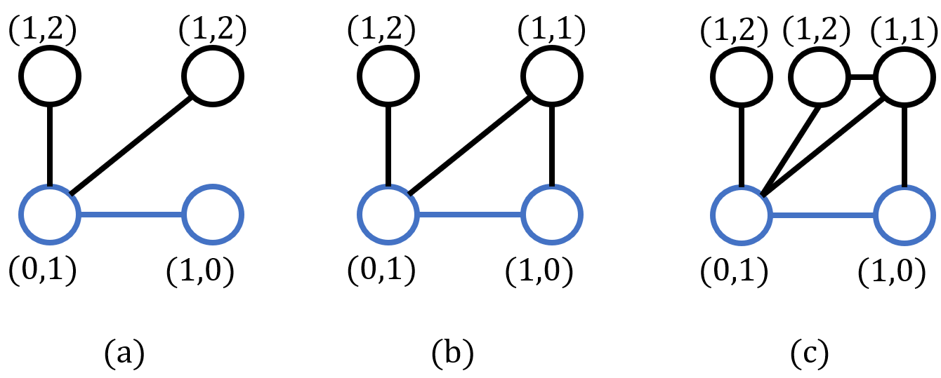
Figure 5: Examples of stars that pass the rooted edges. In these figures, the rooted 2-tuples are colored blue.

A.5 The proof of Theorem 5.3

Below we show the counting power of ESC-GNN in terms of induced subgraph counting. We restate the Theorem 5.3 as follows.

Theorem 5.3.

In terms of induced subgraph counting, ESC-GNN can count (1) up to 4-cycles; (2) up to 4-cliques; (3) up to 4-stars; (4) up to 3-paths.

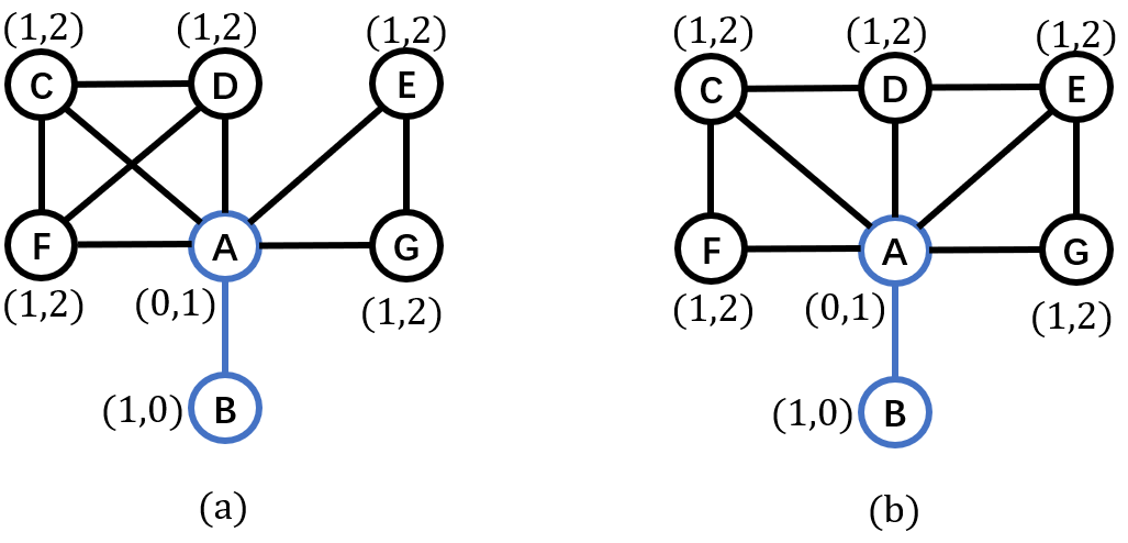
Figure 6: Examples where ESC-GNN cannot induced-subgraph-count 5-stars. In these figures, the rooted 2-tuples are colored blue.

Proof.

Since cliques are fully connected substructures, the proof of cliques is the same as the proof of subgraph counting.

For cycles, the number of 3-cycles is the same as 3-cliques. As for 4-cycles, we only need to consider the situation shown in Figure 3(a), where the number of $(1,2,2,1)$ edges reflects the number of 4-cycles. For induced-subgraph-counting 5-cycles, in Figure 7(a), there is no 5-cycle that pass $AB$, while in Figure 7(b), there is one 5-cycle $ABEDC$ that passes $AB$. However, ESC-GNN cannot differentiate the two graphs since the degree information and the distance information is the same. Therefore, ESC-GNN cannot induced-subgraph-count 5-cycles. It can serve as the same example for not counting 4-paths.

The proof of paths is actually the same as Theorem 5.2.

In terms of 3-stars and 4-stars, we only need to consider the situation shown in Figure 5(a), where the number of $(1,2)$ nodes encodes the number of stars, i.e., denote the number of $(1,2)$ nodes as $N^{\prime}$, the number of $p$-stars ($p\leq 4$) is $C_{N^{\prime}}^{p-2}$.

For 5-stars, a pair of examples are shown in Figure 6. These two graphs will be assigned the same structural embedding since the node degree information, and the distance information among these two graphs are the same. Therefore, ESC-GNN cannot differentiate the two graphs. However, Figure 6(a) contains no 5-star that passes the rooted 2-tuple $AB$, while Figure 6(b) contains one 5-star ($BAFDG$) that passes the rooted 2-tuple $AB$. ∎

Figure 7: Examples where ESC-GNN cannot induced-subgraph-count 5-cycles. In these figures, the rooted 2-tuples are colored blue.

A.6 The proof of Theorem 5.5

Here we restate Theorem 5.5 as follows:

Theorem 5.5.

Consider all pairs of $r$-regular graphs with $n$ nodes, let $3\leq r<(2log2n)^{1/2}$ and $\epsilon$ be a fixed constant. With the hop parameter $h$ set to $\lfloor(1/2+\epsilon)\frac{log2n}{log(r-1)}\rfloor$, there exists an ESC-GNN that can distinguish $1-o(n^{-1/2})$ such pairs of graphs.

Recall that we encode the distance information as augmented structural features for ESC-GNN. For the input graph $G$, denote the node-level distance encoding on $h$-hop subgraphs on 2-tuple $(u,v)$ as $D_{(u,v),G}^{h,\text{node}}$. Note that we can naturally transfer the encoding on 2-tuples to node by: ($D_{v,G}^{h,\text{node}}=D_{(v,v),G}^{h,\text{node}}$). We then introduce the following lemma.

Lemma A.5.

For two graphs $G_{1}=(V_{1},E_{1})$ and $G_{2}=(V^{2},E^{2})$ that are randomly and independently sampled from $r$-regular graphs with n nodes ($3\leq r<(2log2n)^{1/2}$). Select two nodes $v_{1}$ and $v_{2}$ from $G_{1}$ and $G_{2}$ respectively. Let $h=\lfloor(1/2+\epsilon)\frac{log2n}{log(r-1)}\rfloor$ where $\epsilon$ is a fixed constant, $D_{v_{1},G_{1}}^{h,\text{node}}=D_{v_{2},G_{2}}^{h,\text{node}}$ with probability at most $o(n^{-3/2})$.

Proof.

The proof follows from (Bollobás, 1982; Feng et al., 2022). As $D_{v,G}^{h,\text{node}}$ stores exactly the same information as the node configuration used in (Feng et al., 2022), therefore the proof is exactly the same as the proof of Lemma 1 in (Feng et al., 2022).

Based on Lemma A.5, we can prove Theorem 5.5. Given node $v_{1}\in V_{1}$, compare $D_{v_{1},G_{1}}^{h,\text{node}}$ with each $D_{v_{2},G_{2}}^{h,\text{node}}$ where $v_{2}\in V_{2}$. The probability that $D_{v_{1},G_{1}}^{h,\text{node}}\neq D_{v_{2},G_{2}}^{h,\text{node}}$ for all possible $v_{2}\in V_{2}$ is $1-o(n^{-3/2})*n=1-o(n^{-1/2})$. Therefore, ESC-GNN can distinguish $1-o(n^{-1/2})$ such pairs of graphs. ∎

A.7 Experimental Details

Stastics of Datasets. The statistics of all used datasets are available in Table 5.

Table 5: Statistics of the used datasets.

Dataset	Graphs	Avg Nodes	Avg Edges	Task Type	Metric
MUTAG	188	17.9	19.8	Graph Classification	ACC
PTC-MR	349	14.1	14.5	Graph Classification	ACC
ENZYMES	600	32.6	62.1	Graph Classification	ACC
PROTEINS	1113	39.1	72.8	Graph Classification	ACC
IMDB-BINARY	1000	19.8	96.5	Graph Classification	ACC
ZINC-12k	12000	23.2	24.9	Graph Regression	MAE
ogbg-molhiv	41127	25.5	27.5	Graph Classification	AUC-ROC
ogbg-molpcba	437929	26.0	28.1	Graph Classification	AP
QM9	129433	18.0	18.6	Graph Regression	MAE
Synthetic	5000	18.8	31.3	Node Regression	MAE

Experimental details. The baselines and data splittings of our experiments follow from existing works (Zhang & Li, 2021; Huang et al., 2023) and the standard data split setting. For ESC-GNN, we adopt GIN (Xu et al., 2018) as the backbone GNN. In the structural embedding, we use both the shortest path distance and the resistance distance (Lü & Zhou, 2011) as the distance feature. For the hop parameter $h$ we search between 1 to 4, and report the best results. Following existing works (Huang et al., 2023), we use Adam optimizer as the optimizer, and use plateau scheduler with patience 10 and decay factor 0.9. On most datasets, the learning rate is set to 0.001, and the hidden embedding dimension is set to 300. The training epoch is set to 2000 for counting substructures, 400 for QM9, 1000 for ZINC, and 150 for the OGB dataset. Most of the experiments are implemented with two Intel Core i9-7960X processors and 2 NVIDIA 3090 graphics cards. Others (e.g., experiments on the TU dataset) are implemented with two Intel Xeon Gold 5218 processors and 10 NVIDIA 2080TI graphics cards.

A.8 Evaluation on Real-World Datasets.

Molecule Dataset. We evaluate ESC-GNN on various popular real-world molecule datasets, including ZINC (Dwivedi et al., 2020) and the OGB dataset (Hu et al., 2020). ZINC is a dataset of chemical compounds, and the task is graph regression. For the OGB dataset, we use ogbg-molhiv and ogbg-molpcba for evaluation. ogbg-molhiv contains 41K molecules with 2 classes, and ogbg-molpcba contains 438 molecules with 128 classes. The task is to predict to which these molecules belong. We follow the standard evaluation metric and the dataset split, and report the result in Table 6.

Table 6: Evalation on ZINC and OGB datasets.

Dataset	OGBG-Hiv (AUCROC)	OGBG-PCBA (AP)	ZINC
GIN	77.07$\pm$1.49	27.03$\pm$0.23	0.163
PNA	79.05$\pm$1.32	28.38$\pm$0.35	0.188
DGN	79.70$\pm$0.97	28.85$\pm$0.30	0.168
GSN	77.99$\pm$1.00	-	0.115
CIN	80.94$\pm$0.57**	-	0.079
NGNN	78.34$\pm$1.86*	28.32$\pm$0.41*	0.111
GIN-AK+	79.61$\pm$1.19**	29.30$\pm$0.44**	0.080
OSAN	-	-	0.126
SUN	80.03$\pm$0.55	-	0.083
DSS-GNN	76.78$\pm$1.66	-	0.102
I2-GNN	78.68$\pm$0.93	-	0.083
ESC-GNN	78.36$\pm$1.06	28.16$\pm$0.31	0.096

TU datasets. We evaluate the performance of ESC-GNN on the TU datasets (Morris et al., 2020a). The experimental settings follow (Zhang & Li, 2021) for more consistent evaluation standards. Specifically, we uniformly use the 10-fold cross validation framework, with the split ratio of training/validation/test set 0.8/0.1/0.1. The results are available in Table 7. In the table, ESC-GNN (h2) and ESC-GNN (h3) denote ESC-GNN with the hop parameters setting to 2 and 3.

Results. From the tables, we observe that ESC-GNN performs much better than normal MPNNs, comparably with or slightly better than subgraph GNNs rooted at nodes, while performing comparably or slightly less than I²-GNN. This shows that while running much faster than these subgraph GNNs (shown in Table 4), ESC-GNN manages to preserve the representation power of subgraph GNNs.

Table 7: Experiments on TU, Accuracy as the evaluation metric.

Dataset	MUTAG	PTC-MR	PROTEINS	ENZYMES	IMDB-B
GIN	84.5$\pm$8.9	51.2$\pm$9.2	70.6$\pm$4.3	38.3$\pm$6.4	73.3$\pm$4.7
PPGN	84.7$\pm$8.2	55.0$\pm$6.4	74.8$\pm$3.3	55.0$\pm$6.4	71.5$\pm$5.4
NGNN	87.9$\pm$8.2*	54.1$\pm$7.7*	73.9$\pm$5.1*	29.0$\pm$8.0*	73.1$\pm$5.7
GIN-AK+	88.8$\pm$4.0	60.5$\pm$8.0	75.5$\pm$4.4	58.9$\pm$6.2	72.4$\pm$3.7
SUN	86.1$\pm$6.0	60.2$\pm$7.2	72.1$\pm$3.8	16.7$\pm$0.0	73.7$\pm$2.9
I2-GNN	87.9$\pm$4.3	61.4$\pm$8.7	74.8$\pm$2.9	40.3$\pm$6.7	73.6$\pm$4.0
ESC-GNN (h2)	86.2$\pm$7.9	52.9$\pm$6.4	73.3$\pm$4.1	53.2$\pm$8.1	72.0$\pm$6.0
ESC-GNN (h3)	85.6$\pm$7.9	56.4$\pm$6.9	76.0$\pm$4.5	43.3$\pm$6.0	73.7$\pm$4.8

A.9 Ablation Study.

We evaluate the effectiveness of each part of the proposed structural embedding on the substructure counting dataset. For the proposed three types of structural embedding (the degree encoding, the node-level distance encoding, and the edge-level distance encoding), we delete one of them from the original structural embedding every time and report the results in Table 8. We observe that after removing the three types of embedding, ESC-GNN performs worse compared with its original version, especially after removing the edge-level distance encoding. This is consistent with our theoretical results: in Theorem 4.4, we show that the proposed structural embedding contains key information for the counting power of subgraph GNNs; in Theorem 5.2 and Theorem 5.3, we show that the edge-level distance information directly encodes the number of certain types of substructures.

Table 8: Ablation study on the proposed structural embedding (norm MAE).

Dataset	Tailed Triangle	Chordal Cycle	4-Clique	4-Path	Triangle-Rectangle	3-cycles	4-cycles	5-cycles	6-cycles
MPNN	0.3631	0.3114	0.1645	0.1592	0.3018	0.3515	0.2742	0.2088	0.1555
ESC-GNN	0.0052	0.0169	0.0064	0.0254	0.0748	0.0074	0.0096	0.0356	0.0578
(- degree)	0.0121	0.0492	0.0106	0.0322	0.0841	0.0342	0.0144	0.0513	0.0652
(- node-level dist)	0.0382	0.0344	0.0222	0.0428	0.1120	0.0157	0.0261	0.0492	0.0608
(- edge-level dist)	0.0208	0.2811	0.0497	0.0584	0.2438	0.2617	0.2244	0.1654	0.1364

References

- Abboud et al. (2021) Abboud, R., Ceylan, I., Grohe, M., and Lukasiewicz, T. The surprising power of graph neural networks with random node initialization. International Joint Conferences on Artificial Intelligence Organization, 2021.
- Abu-El-Haija et al. (2019) Abu-El-Haija, S., Perozzi, B., Kapoor, A., Alipourfard, N., Lerman, K., Harutyunyan, H., Ver Steeg, G., and Galstyan, A. Mixhop: Higher-order graph convolutional architectures via sparsified neighborhood mixing. In international conference on machine learning, pp. 21–29. PMLR, 2019.
- Arvind et al. (2020) Arvind, V., Fuhlbrück, F., Köbler, J., and Verbitsky, O. On weisfeiler-leman invariance: Subgraph counts and related graph properties. Journal of Computer and System Sciences, 113:42–59, 2020.
- Babai et al. (1980) Babai, L., Erdos, P., and Selkow, S. M. Random graph isomorphism. SIaM Journal on computing, 9(3):628–635, 1980.
- Balcilar et al. (2021) Balcilar, M., Héroux, P., Gauzere, B., Vasseur, P., Adam, S., and Honeine, P. Breaking the limits of message passing graph neural networks. In International Conference on Machine Learning, pp. 599–608. PMLR, 2021.
- Barceló et al. (2021) Barceló, P., Geerts, F., Reutter, J., and Ryschkov, M. Graph neural networks with local graph parameters. Advances in Neural Information Processing Systems, 34:25280–25293, 2021.
- Bevilacqua et al. (2022) Bevilacqua, B., Frasca, F., Lim, D., Srinivasan, B., Cai, C., Balamurugan, G., Bronstein, M. M., and Maron, H. Equivariant subgraph aggregation networks. In International Conference on Learning Representations, 2022.
- Bodnar et al. (2021a) Bodnar, C., Frasca, F., Otter, N., Wang, Y., Lio, P., Montufar, G. F., and Bronstein, M. Weisfeiler and lehman go cellular: Cw networks. Advances in Neural Information Processing Systems, 34:2625–2640, 2021a.
- Bodnar et al. (2021b) Bodnar, C., Frasca, F., Wang, Y., Otter, N., Montufar, G. F., Lio, P., and Bronstein, M. Weisfeiler and lehman go topological: Message passing simplicial networks. In International Conference on Machine Learning, pp. 1026–1037. PMLR, 2021b.
- Bollobás (1982) Bollobás, B. Distinguishing vertices of random graphs. In North-Holland Mathematics Studies, volume 62, pp. 33–49. Elsevier, 1982.
- Bouritsas et al. (2022) Bouritsas, G., Frasca, F., Zafeiriou, S. P., and Bronstein, M. Improving graph neural network expressivity via subgraph isomorphism counting. IEEE Transactions on Pattern Analysis and Machine Intelligence, 2022.
- Cai et al. (1992) Cai, J.-Y., Fürer, M., and Immerman, N. An optimal lower bound on the number of variables for graph identification. Combinatorica, 12(4):389–410, 1992.
- Chen et al. (2020) Chen, Z., Chen, L., Villar, S., and Bruna, J. Can graph neural networks count substructures? Advances in neural information processing systems, 33:10383–10395, 2020.
- Cotta et al. (2021) Cotta, L., Morris, C., and Ribeiro, B. Reconstruction for powerful graph representations. Advances in Neural Information Processing Systems, 34:1713–1726, 2021.
- Deshpande et al. (2002) Deshpande, M., Kuramochi, M., and Karypis, G. Automated approaches for classifying structures. Technical report, MINNESOTA UNIV MINNEAPOLIS DEPT OF COMPUTER SCIENCE, 2002.
- Dwivedi et al. (2020) Dwivedi, V. P., Joshi, C. K., Laurent, T., Bengio, Y., and Bresson, X. Benchmarking graph neural networks. arXiv preprint arXiv:2003.00982, 2020.
- Dwivedi et al. (2021) Dwivedi, V. P., Luu, A. T., Laurent, T., Bengio, Y., and Bresson, X. Graph neural networks with learnable structural and positional representations. In International Conference on Learning Representations, 2021.
- Feng et al. (2022) Feng, J., Chen, Y., Li, F., Sarkar, A., and Zhang, M. How powerful are k-hop message passing graph neural networks. arXiv preprint arXiv:2205.13328, 2022.
- Frasca et al. (2022) Frasca, F., Bevilacqua, B., Bronstein, M. M., and Maron, H. Understanding and extending subgraph gnns by rethinking their symmetries. In Advances in Neural Information Processing Systems, 2022.
- Fürer (2017) Fürer, M. On the combinatorial power of the weisfeiler-lehman algorithm. In International Conference on Algorithms and Complexity, pp. 260–271. Springer, 2017.
- Geerts (2020) Geerts, F. The expressive power of kth-order invariant graph networks. arXiv preprint arXiv:2007.12035, 2020.
- Grohe & Otto (2015) Grohe, M. and Otto, M. Pebble games and linear equations. The Journal of Symbolic Logic, 80(3):797–844, 2015. doi: 10.1017/jsl.2015.28.
- Hu et al. (2020) Hu, W., Fey, M., Zitnik, M., Dong, Y., Ren, H., Liu, B., Catasta, M., and Leskovec, J. Open graph benchmark: Datasets for machine learning on graphs. Advances in neural information processing systems, 33:22118–22133, 2020.
- Huang et al. (2023) Huang, Y., Peng, X., Ma, J., and Zhang, M. Boosting the cycle counting power of graph neural networks with i2-gnns. 2023.
- Jiang et al. (2010) Jiang, C., Coenen, F., and Zito, M. Finding frequent subgraphs in longitudinal social network data using a weighted graph mining approach. In International Conference on Advanced Data Mining and Applications, pp. 405–416. Springer, 2010.
- Jin et al. (2018) Jin, W., Barzilay, R., and Jaakkola, T. Junction tree variational autoencoder for molecular graph generation. In International conference on machine learning, pp. 2323–2332. PMLR, 2018.
- Kipf & Welling (2017) Kipf, T. N. and Welling, M. Semi-supervised classification with graph convolutional networks. In 5th International Conference on Learning Representations, ICLR 2017, Toulon, France, April 24-26, 2017, Conference Track Proceedings. OpenReview.net, 2017. URL https://openreview.net/forum?id=SJU4ayYgl.
- Koyutürk et al. (2004) Koyutürk, M., Grama, A., and Szpankowski, W. An efficient algorithm for detecting frequent subgraphs in biological networks. Bioinformatics, 20(suppl_1):i200–i207, 2004.
- Kreuzer et al. (2021) Kreuzer, D., Beaini, D., Hamilton, W., Létourneau, V., and Tossou, P. Rethinking graph transformers with spectral attention. Advances in Neural Information Processing Systems, 34:21618–21629, 2021.
- Langley (2000) Langley, P. Crafting papers on machine learning. In Langley, P. (ed.), Proceedings of the 17th International Conference on Machine Learning (ICML 2000), pp. 1207–1216, Stanford, CA, 2000. Morgan Kaufmann.
- Li et al. (2020) Li, P., Wang, Y., Wang, H., and Leskovec, J. Distance encoding: Design provably more powerful neural networks for graph representation learning. Advances in Neural Information Processing Systems, 33:4465–4478, 2020.
- Lim et al. (2022) Lim, D., Robinson, J. D., Zhao, L., Smidt, T., Sra, S., Maron, H., and Jegelka, S. Sign and basis invariant networks for spectral graph representation learning. In ICLR 2022 Workshop on Geometrical and Topological Representation Learning, 2022.
- Liu & Song (2022) Liu, X. and Song, Y. Graph convolutional networks with dual message passing for subgraph isomorphism counting and matching. In Proceedings of the AAAI Conference on Artificial Intelligence, volume 36, pp. 7594–7602, 2022.
- Liu et al. (2020) Liu, X., Pan, H., He, M., Song, Y., Jiang, X., and Shang, L. Neural subgraph isomorphism counting. In Proceedings of the 26th ACM SIGKDD International Conference on Knowledge Discovery & Data Mining, pp. 1959–1969, 2020.
- Loukas (2020) Loukas, A. How hard is to distinguish graphs with graph neural networks? Advances in neural information processing systems, 33:3465–3476, 2020.
- Lü & Zhou (2011) Lü, L. and Zhou, T. Link prediction in complex networks: A survey. Physica A: statistical mechanics and its applications, 390(6):1150–1170, 2011.
- Maron et al. (2018) Maron, H., Ben-Hamu, H., Shamir, N., and Lipman, Y. Invariant and equivariant graph networks. In International Conference on Learning Representations, 2018.
- Maron et al. (2019) Maron, H., Ben-Hamu, H., Serviansky, H., and Lipman, Y. Provably powerful graph networks. Advances in neural information processing systems, 32, 2019.
- Morris et al. (2019) Morris, C., Ritzert, M., Fey, M., Hamilton, W. L., Lenssen, J. E., Rattan, G., and Grohe, M. Weisfeiler and leman go neural: Higher-order graph neural networks. In Proceedings of the AAAI conference on artificial intelligence, pp. 4602–4609, 2019.
- Morris et al. (2020a) Morris, C., Kriege, N. M., Bause, F., Kersting, K., Mutzel, P., and Neumann, M. Tudataset: A collection of benchmark datasets for learning with graphs. arXiv preprint arXiv:2007.08663, 2020a.
- Morris et al. (2020b) Morris, C., Rattan, G., and Mutzel, P. Weisfeiler and leman go sparse: Towards scalable higher-order graph embeddings. Advances in Neural Information Processing Systems, 33:21824–21840, 2020b.
- Murphy et al. (2019) Murphy, R., Srinivasan, B., Rao, V., and Ribeiro, B. Relational pooling for graph representations. In International Conference on Machine Learning, pp. 4663–4673. PMLR, 2019.
- Nikolentzos et al. (2020) Nikolentzos, G., Dasoulas, G., and Vazirgiannis, M. k-hop graph neural networks. Neural Networks, 130:195–205, 2020.
- Papp & Wattenhofer (2022) Papp, P. A. and Wattenhofer, R. A theoretical comparison of graph neural network extensions. arXiv preprint arXiv:2201.12884, 2022.
- Papp et al. (2021) Papp, P. A., Martinkus, K., Faber, L., and Wattenhofer, R. Dropgnn: random dropouts increase the expressiveness of graph neural networks. Advances in Neural Information Processing Systems, 34:21997–22009, 2021.
- Preciado & Jadbabaie (2010) Preciado, V. M. and Jadbabaie, A. From local measurements to network spectral properties: Beyond degree distributions. In 49th IEEE Conference on Decision and Control (CDC), pp. 2686–2691. IEEE, 2010.
- Qian et al. (2022) Qian, C., Rattan, G., Geerts, F., Niepert, M., and Morris, C. Ordered subgraph aggregation networks. In Advances in Neural Information Processing Systems, 2022.
- Ramakrishnan et al. (2014) Ramakrishnan, R., Dral, P. O., Rupp, M., and Von Lilienfeld, O. A. Quantum chemistry structures and properties of 134 kilo molecules. Scientific data, 1(1):1–7, 2014.
- Sandfelder et al. (2021) Sandfelder, D., Vijayan, P., and Hamilton, W. L. Ego-gnns: Exploiting ego structures in graph neural networks. In ICASSP 2021-2021 IEEE International Conference on Acoustics, Speech and Signal Processing (ICASSP), pp. 8523–8527. IEEE, 2021.
- Shervashidze et al. (2009) Shervashidze, N., Vishwanathan, S., Petri, T., Mehlhorn, K., and Borgwardt, K. Efficient graphlet kernels for large graph comparison. In Artificial intelligence and statistics, pp. 488–495. PMLR, 2009.
- Tahmasebi et al. (2020) Tahmasebi, B., Lim, D., and Jegelka, S. Counting substructures with higher-order graph neural networks: Possibility and impossibility results. arXiv preprint arXiv:2012.03174, 2020.
- Veličković et al. (2019) Veličković, P., Ying, R., Padovano, M., Hadsell, R., and Blundell, C. Neural execution of graph algorithms. arXiv preprint arXiv:1910.10593, 2019.
- Vignac et al. (2020) Vignac, C., Loukas, A., and Frossard, P. Building powerful and equivariant graph neural networks with structural message-passing. Advances in Neural Information Processing Systems, 33:14143–14155, 2020.
- Weisfeiler & Leman (1968) Weisfeiler, B. and Leman, A. The reduction of a graph to canonical form and the algebra which appears therein. NTI, Series, 2(9):12–16, 1968.
- Wu et al. (2018) Wu, Z., Ramsundar, B., Feinberg, E. N., Gomes, J., Geniesse, C., Pappu, A. S., Leswing, K., and Pande, V. Moleculenet: a benchmark for molecular machine learning. Chemical science, 9(2):513–530, 2018.
- Wu et al. (2020) Wu, Z., Pan, S., Chen, F., Long, G., Zhang, C., and Philip, S. Y. A comprehensive survey on graph neural networks. IEEE transactions on neural networks and learning systems, 32(1):4–24, 2020.
- Xhonneux et al. (2021) Xhonneux, L.-P., Deac, A.-I., Veličković, P., and Tang, J. How to transfer algorithmic reasoning knowledge to learn new algorithms? Advances in Neural Information Processing Systems, 34:19500–19512, 2021.
- Xu et al. (2018) Xu, K., Hu, W., Leskovec, J., and Jegelka, S. How powerful are graph neural networks? In International Conference on Learning Representations, 2018.
- Yan et al. (2021) Yan, Z., Ma, T., Gao, L., Tang, Z., and Chen, C. Link prediction with persistent homology: An interactive view. In International Conference on Machine Learning, pp. 11659–11669. PMLR, 2021.
- Yan et al. (2022) Yan, Z., Ma, T., Gao, L., Tang, Z., Wang, Y., and Chen, C. Neural approximation of graph topological features. In Oh, A. H., Agarwal, A., Belgrave, D., and Cho, K. (eds.), Advances in Neural Information Processing Systems, 2022.
- You et al. (2021) You, J., Gomes-Selman, J. M., Ying, R., and Leskovec, J. Identity-aware graph neural networks. In Proceedings of the AAAI Conference on Artificial Intelligence, pp. 10737–10745, 2021.
- Yu et al. (2023) Yu, X., Liu, Z., Fang, Y., and Zhang, X. Learning to count isomorphisms with graph neural networks. arXiv preprint arXiv:2302.03266, 2023.
- Zhang & Chen (2018) Zhang, M. and Chen, Y. Link prediction based on graph neural networks. Advances in neural information processing systems, 31, 2018.
- Zhang & Li (2021) Zhang, M. and Li, P. Nested graph neural networks. Advances in Neural Information Processing Systems, 34:15734–15747, 2021.
- Zhang et al. (2021) Zhang, M., Li, P., Xia, Y., Wang, K., and Jin, L. Labeling trick: A theory of using graph neural networks for multi-node representation learning. Advances in Neural Information Processing Systems, 34:9061–9073, 2021.
- Zhao et al. (2022) Zhao, L., Jin, W., Akoglu, L., and Shah, N. From stars to subgraphs: Uplifting any gnn with local structure awareness. In International Conference on Learning Representations, 2022.
- Zhou et al. (2020) Zhou, J., Cui, G., Hu, S., Zhang, Z., Yang, C., Liu, Z., Wang, L., Li, C., and Sun, M. Graph neural networks: A review of methods and applications. AI Open, 1:57–81, 2020.