High-Frequency Volatility Estimation with Fast Multiple Change Points Detection

Abstract

We propose high-frequency volatility estimators with multiple change points that are $\ell_{1}$-regularized versions of two classical estimators: quadratic variation and bipower variation. We establish consistency of these estimators for the true unobserved volatility and the change points locations under general sub-Weibull distribution assumptions on the jump process. The proposed estimators employ the computationally efficient least angle regression algorithm for estimation purposes, followed by a reduced dynamic programming step to refine the final number of change points. In terms of numerical performance, the proposed estimators are computationally fast and accurately identify breakpoints near the end of the sample, which is highly desirable in today’s electronic trading environment. In terms of out-of-sample volatility prediction, our new estimators provide more realistic and smoother volatility forecasts, and they outperform a wide range of classical and recent volatility estimators across various frequencies and forecasting horizons.

Keywords: Bipower Variation; Change Points; High-Frequency; Trend Filter; Volatility Estimation.
JEL Classification: C14, C15, C58, D53, G17

1 Introduction

Change points detection algorithms, also known as temporal signal segmentation, are widely studied in machine learning and signal processing applications like audio, speech and image processing, network intrusion detection, climate change detection, and EEG segmentation (Radke et al., , 2005; Reeves et al., , 2007; Harchaoui et al., , 2009; Safikhani et al., , 2021). Breakpoints are abrupt variations in the data-generating process. There is extensive literature on developing different techniques for changes in the mean (Levy-Leduc and Harchaoui, 2007; Zou et al., 2014; Li et al., 2015; Arlot et al., 2019; Alanqary et al., 2021; Kaul et al., 2021; Wang et al., 2021); or more general non-parametric change point detection in a sequence of cumulative distribution functions as recently proposed in Horváth et al., (2021). Other change point detection algorithms include nonparametric approaches by Zou et al., (2014), Arlot et al., (2019); sparsified binary segmentation by Cho and Fryzlewicz, (2015) and CUSUM-based methods by Alanqary et al., (2021). Iacus and Yoshida, (2010) compares the least squares method, CUSUM method, and quasi maximum likelihood approach for discretely sampled stochastic differential equations.

Regarding change points in financial modeling, Bibinger et al., (2017) propose methods to test the presence of jumps and change points in the volatility process and analyze the roughness of the volatility. Li and Xing, (2022) uses a proposed change point intensity model to measure quote volatility. Spokoiny, (2009) develops a multi-scale local change point detection method with applications to value-at-risk. Li et al., (2021) propose a Markov-Switching Autoregressive Conditional Intensity model, which divides daily volatility into two regimes - dominant and minor. Shi and Ho, (2015) propose adaptive-FIGARCH and time-varying FIGARCH to incorporate structural changes as a function of time. Finally, Mercurio and Spokoiny, (2004) introduce a new framework for estimating the interval of time homogeneity of volatility models called Locally Adaptive Volatility Estimate.

This paper focuses on multiple change points detection in the variance process. Under very general noise distribution assumptions, we show how estimators introduced by Levy-Leduc and Harchaoui, (2007) and Harchaoui and Lévy-Leduc, (2010) can be naturally extended to consistently detect structural breaks not only in the observed signal but also in a latent process such as the spot volatility of high-frequency financial returns.

A piecewise-constant spot volatility process with an unknown number of breakpoints was first analyzed by Fryzlewicz et al., (2006) using a wavelet thresholding algorithm. They showed that piecewise volatility estimation is more accurate in long- and short-term volatility forecasts than in the GARCH$(1,1)$ and simple moving window techniques—a result also confirmed by our methods in the empirical section below. Similarly, as Harchaoui and Lévy-Leduc, (2010), we recast the multiple change-point estimation problem as a variable selection problem: we use the Least Angle Regression (LARS) algorithm from Efron et al., (2004), and the Dynamic Programming (DP) step to implement the Least Square Total Variation (LSTV^∗) algorithm for breakpoint location detection, and simultaneous estimation of the latent spot volatility process. The theory for the proposed estimators is developed under a general sub-Weibull noise assumption that is more natural in the context of heavy-tailed financial data than the typically assumed sub-Gaussianity. We provide non-asymptotic results in the form of probabilistic bounds with general rates and consistency for breakpoint locations and the integrated variance process under infill asymptotics.

The main contributions of our paper consist of developing a new multiple change points detection algorithm for the high-frequency spot volatility process. Our algorithm uses increments of the corresponding consistent estimator of the integrated volatility. We show that it inherits the theoretical guarantees for the consistency of breakpoints location and volatility estimation from the consistency of the original high-frequency volatility estimator without structural breaks. By doing so, we extend the consistency results proposed by Levy-Leduc and Harchaoui, (2007) to the given latent process—the spot volatility of high-frequency returns—and we prove it under more general sub-Weibull distribution assumptions on the jump process. Empirically, we show that the forecasting performance of the proposed estimator is much better than a broad spectrum of different volatility models often used in practice for all of the data frequencies and one-step-ahead and daily forecasting horizon periods. In particular, the proposed high-frequency volatility estimator outperforms classical QV and BV by Barndorff-Nielsen and Shephard, (2004); more recent refinements such as realized volatility and bipower variation (RVB) and realized volatility and quarticity (RVQ) by Yu, (2020); the heavy-tailed $t$-GARCH model with Student-$t$ innovations; the long-memory extension of it—the $t$-FIGARCH model from Shi and Ho, (2015); and, finally, the mixed-frequency approach—the HAR model from Corsi, (2009), where the HAR model is used only for multi-step (daily) volatility forecast.

In Section 2, we introduce realized variance estimators and present the main assumptions and formulation of the model featuring the piecewise-constant spot volatility process. Section 4 outlines our consistency results. In Section 5, we present empirical examples using simulated and real data. Section 6 highlights the versatility and practical application of our proposed volatility estimators. Finally, in Section 7, we conclude. The appendices provide supplementary information, including details on the sub-Weibull distribution, a comparison between the direct and our indirect LSTV algorithm, proofs of all the theorems, technical lemmas, and non-asymptotic results for breakpoint location.

2 High-Frequency Volatility Modeling

2.1 Price Dynamics and Volatility Estimators

Let $p(t)$ denote the stochastic process representing the $log$-price of an asset at time $t\geq 0$. As shown in Delbaen and Schachermayer, (1994), under the assumption of no arbitrage, $p(t)$ must be a semi-martingale ($p\in\mathcal{SM}$), For all $p\in\mathcal{SM}$, the quadratic variation (QV) process can be defined as a probability limit of the sum

$$\left[p\right](t)=\operatorname*{\mathit{p}-\lim}_{n\to\infty}\sum_{j=0}^{n-1}\left(p\left(t_{j+1}\right)-p\left(t_{j}\right)\right)^{2},$$ (1)

for any sequence of partitions $t_{0}=0<t_{1}<\ldots<t_{n}=t$ with $\sup_{j}(t_{j+1}-t_{j})\to 0$ for $n\to\infty$.
When we choose the partition to be equally spaced; i.e. $t_{j}=jt/n$ for all $j$, then the QV is the sum of the corresponding squared $\log$-returns $r^{2}_{1,t},\ldots,r^{2}_{n,t}$.

Example 2.1.

Consider the stock prices dynamics given by the Merton Jump Diffusion (MJD) process

$$\mbox{d}p_{t}=p_{t}\left[(\mu(t)-\mu_{J}\nu)\mbox{d}t+\sigma(t)\mbox{d}W_{t}+\mbox{d}\sum^{N_{t}}_{i=1}Q_{i}\right],$$

where $\mu(t)$ and $\sigma(t)$ are drift and spot volatility, respectively, $W_{t}$ is a standard Brownian motion, and $\sum^{N_{t}}_{i=1}Q_{i}$ is a compound Poisson process with normal distributed jumps $Q_{i}\overset{i.i.d.}{\sim}N(\mu_{J},\sigma^{2}_{J})$ and intensity $N_{t}\sim\mathrm{Poisson}(\nu)$, where $\sim$ denotes distributional equivalence. The two processes are independent and adapted to the filtration $\{\mathcal{F}_{t}\}_{t\geq 0}$, associated with the Brownian motion $\{W_{t}\}_{t\geq 0}$. Hence, by using Itô isometry for the jump process, one gets

$$[p](t)=\int_{0}^{t}\sigma^{2}(s)\mbox{d}s+\sum^{N_{t}}_{i=1}Q_{i}^{2}.$$

the sum of integrated variance and the aggregated squared jump components.

The integrated variance of the returns has both a continuous component as well as a quadratic variation of the jumps part. The high-frequency $log$-returns allow us to compute the realized variance (RV)

$$[p](t)=\sum_{j=1}^{n}\left(p(jt/n)-p((j-1)t/n)\right)^{2}=\sum_{j=1}^{n}r^{2}_{j,t}.$$

We also consider the power variation which is a jump robust estimator introduced in Barndorff-Nielsen and Shephard, (2004),

$$[p]^{[r,s]}(t)=\left(\frac{1}{n}\right)^{1-\frac{r+s}{2}}\sum^{n}_{j=2}\left\lvert r_{j,t}\right\rvert^{r}\left\lvert r_{j-1,t}\right\rvert^{s}.$$ (2)

In particular, for $r=s=1$, the above equation reduces to the bi-power variation (BV). Barndorff-Nielsen and Shephard, (2004) proved that, in the case of a finite number of jumps, in a high-frequency setting under infill-asymptotics, the realized power variation of the returns converges to the Semi Martingale Stochastic Volatility (SMSV) process.

In the absence of price jumps, i.e., when all the $Q_{i}$’s are identical $0$, and assuming a frictionless market, we have

$$dp(t)=p_{t}\left[\mu(t)dt+\sigma(t)dW(t)\right].$$

In this case, realized variance is a consistent estimator for the integrated volatility

$$\operatorname*{\mathit{p}-\lim}_{n\rightarrow+\infty}\sum_{i=1}^{n}r^{2}_{i,t}=\int_{0}^{t}\sigma^{2}(s)ds.$$

2.2 MJD with Sub-Weibull Jumps

The normality assumption on the distributed jumps $Q_{1},Q_{2},\ldots$ in Example 2.1 above is a special case of a more general class of random variables. Indeed, Gaussian random variables are sub-Weibull with tail decay parameter $\alpha=2$. In the sequel, we assume our $Q_{j}$’s to be sub-Weibull with $\alpha>0$. In addition, we assume that the jump component in the stock price dynamics is given by a Lévy process $\{\mathfrak{X}_{t}\}_{t\geq 0}$ with non-negative integer values. As in the case of classical MJD, we assume that the processes are independent and adapted to the filtration associated with the Brownian motion $\{W_{t}\}_{t\geq 0}$.
This particular assumption allows us to model the price jumps as being heavy-tailed. (See Appendix A about sub-Weibull random variables.) We do however remain in the context of finite jump activity. This will allow us to deal with the fact that the jump process is not centered. We note that the quadratic variation theory and volatility estimation theory that follows from it remain unchanged by this assumption.

2.3 Volatility Estimators and Consistency Conditions

Recall that by the results of Barndorff-Nielsen and Shephard, (2002), we have

$$\operatorname*{\mathit{p}-\lim}_{n^{*}\rightarrow+\infty}\left[\sum_{i=1}^{n^{*}}r^{2}_{i,t}-\left(\int_{0}^{t}\sigma^{2}(s)\mbox{d}s+\sum^{N_{t}}_{i=1}Q_{i}^{2}\right)\right]=0\text{ and }$$

$$\operatorname*{\mathit{p}-\lim}_{n^{*}\rightarrow+\infty}\left(\sum_{i=1}^{n^{*}-1}\left\lvert r_{i,t}\right\rvert\left\lvert r_{i+1,t}\right\rvert-\int_{0}^{t}\sigma^{2}(s)\mbox{d}s\right)=0,$$

under the MJD model, where $n^{*}$ denotes the number of samples.
We can combine both conditions under a general framework that is conducive to change point detection. Indeed, let $\mathbf{r}_{t}=(r_{1,t},\cdots,r_{n^{*},t})$ denote the vector of returns, and let $F$ denote a transformation of $\mathbf{r}_{t}$, with $F(\mathbf{r}_{t})$ being a vector of length $n$ which depends on $n^{*}$. Here, $t\in(0,T]$ for some time horizon $T$. In particular, $n$ grows to $+\infty$ as $n^{*}$ grows to $+\infty$. In what follows, we consider $F_{\text{RV}}$ and $F_{\text{BP}}$, corresponding to realized variance and bi-power variation, respectively, and defined as

$$F_{\text{RV}}(\mathbf{r}_{t}) =\mathbf{r}_{t}\circ\mathbf{r}_{t}=\left(r^{2}_{1,t},\cdots,r^{2}_{n^{*},t}\right),\text{ and }$$

$$F_{\text{BP}}(\mathbf{r}_{t}) =\left\lvert\mathbf{r}_{t,[1:n^{*}-1]}\right\rvert\circ\left\lvert\mathbf{r}_{t,[2:n^{*}]}\right\rvert=\left(|r_{1,t}||r_{2,t}|,\cdots,|r_{n^{*}-1,t}||r_{n^{*},t}|\right),$$ (3)

where $\left\lvert\mathbf{r}_{t,[a:b]}\right\rvert$ denotes the truncated vector of absolute values of returns $(\left\lvert r_{a,t}\right\rvert,\cdots,\left\lvert r_{b,t}\right\rvert)$, and $\circ$ denotes the Hadamard product. Clearly, for $F_{\text{RV}}$, $n=n^{*}$ and for $F_{\text{BP}}$, $n=n^{*}-1$. In the sequel, $F$ will just denote either transformation.
Using Riemann sums, we see that

$$\int_{0}^{t}\sigma^{2}(s)ds=\lim_{n\rightarrow+\infty}\sum_{i=1}^{n}\dfrac{t}{n}\sigma^{2}(\tau_{i,t}),$$

where $(i-1)t/n\leq\tau_{i,t}\leq it/n$ and $i=1,\cdots,n$. This allows us to rewrite our consistency conditions after defining a few variables.
First, we define the jump-corruption variables $\varepsilon_{J,1,t},\cdots,\varepsilon_{J,n,t}$ as

$$\varepsilon_{J,i,t}:=\sum_{j=\mathfrak{X}_{\tau_{i-1,t}}+1}^{\mathfrak{X}_{\tau_{i,t}}}Q^{2}_{j}\sim\sum_{j=1}^{\mathfrak{X}_{\tau_{i,t}}-\mathfrak{X}_{\tau_{i-1,t}}}Q^{2}_{j}\sim\sum_{j=1}^{\mathfrak{X}_{t/n}}Q^{2}_{j}.$$

Next, we define

$$y_{t,i}=\dfrac{t}{n}\sigma^{2}(\tau_{i,t})+\chi_{J}\left(1-\chi_{R}\right)\varepsilon_{J,i,t}.$$

Here, $\chi_{J}\in\left\{0,1\right\}$ is an indicator function that equals $1$ if the price process has jumps and $0$ otherwise; while $\chi_{R}\in\left\{0,1\right\}$ is an indicator function that equals $1$ if $F$ is jump-robust, and $0$ otherwise.
Combining these observations, we have the general consistency condition:

$$\operatorname*{\mathit{p}-\lim}_{n\rightarrow+\infty}\sum_{i=1}^{n}\left(F(\mathbf{r}_{t})_{i}-y_{t,i}\right)=0.$$ (4)

In fact, (4) implies that the vector $F(\mathbf{r}_{t})$ converges to the vector $\mathbf{Y}_{t}$ in probability with respect to MSE. Here, $\mathbf{Y}_{t}:=(y_{t,1},\cdots,y_{t,n})$

Proposition 2.2.

If (4) holds, then $\operatorname*{\mathit{p}-\lim}_{n\rightarrow+\infty}\dfrac{1}{n}\left\lVert F(\mathbf{r}_{t})-\mathbf{Y}_{t}\right\rVert^{2}_{2}=0.$

With this proposition at hand, we can define the following function capturing the rate of convergence of $F(\mathbf{r}_{t})-\mathbf{Y}_{t}$ to $0$ in probability with respect to MSE:

$$\mathfrak{p}_{n}(\rho):=\mathbb{P}\left(\dfrac{1}{n}\left\lVert F(\mathbf{r}_{t})-\mathbf{Y}_{t}\right\rVert^{2}_{2}>\rho\right).$$

This rate of convergence is important as it will appear in a number of our consistency results in the sequel.

3 Change Point Detection with $\ell_{1}$-Regularization

3.1 The LASSO Model

We are interested in detecting changes in the continuous part of the square spot volatility, $\sigma^{2}$. We assume the spot volatility to have $K^{*}$ change points $\tau^{*}_{1,t},\cdots,\tau^{*}_{K^{*},t}$ between $\tau^{*}_{0,t}:=0$ and $\tau^{*}_{K^{*}+1,t}:=t$. Since we cannot observe the volatility, our approach will use the components of the vector of transformed returns $F(\mathbf{r}_{t})$ as a proxy for the spot volatility. In particular, we will take our $\tau_{i,t}$’s to be $\tau_{i,t}:=(i-1)t/n$, $i=1,\cdots,n$ so that they are equally spaced and allow us to compute the returns easily. We are thus interested in detecting the change point locations $\tau^{*}_{k,t}$ in the following model

$$y_{t,i}:=\dfrac{t}{n}\sigma^{2}(\tau^{*}_{k,t})+\chi_{J}(1-\chi_{R})\varepsilon_{J,i,t}$$ (5)

for $k=0,\cdots,K^{*}+1$ and $i=1,\cdots,n$, indirectly using the proxy $F(\mathbf{r}_{t})$ in view of the consistency condition (4).

We can rewrite the model in vector form as

$$\mathbf{Y}_{t}=\mathbf{X}\boldsymbol{\beta}^{*}_{\sigma}+\chi_{J}\left(1-\chi_{R}\right)\mathfrak{E}_{J,t}.$$ (6)

Here, $\mathbf{X}$ denotes the $n\times n$ lower triangular matrix with nonzero elements equal to $1$, $\mathfrak{E}_{J,t}:=(\varepsilon_{J,1,t},...,\varepsilon_{J,n,t})^{T}$, and the $n\times 1$ vector $\boldsymbol{\beta}^{*}_{\sigma}$ is ones whose components are equal to $0$ except those corresponding to the change point instants.

Normally, in change points detection problem using $\ell_{1}$ regularization, our goal would be to solve the following Least Squares with Total Variation penalty (LSTV) problem

$$\operatorname*{argmin}_{\boldsymbol{\beta}\in\mathbb{R}^{n}}\mathcal{L}_{\sigma}(\boldsymbol{\beta})$$ (7)

$$\mbox{where }\mathcal{L}_{\sigma}(\boldsymbol{\beta}) :=\frac{1}{n}\left\lVert\dfrac{t}{n}\boldsymbol{\sigma}^{2}_{t}-\mathbf{X}\boldsymbol{\beta}\right\rVert^{2}_{2}+\lambda\left\lVert\boldsymbol{\beta}\right\rVert_{1}$$

$$:=\frac{1}{n}\sum_{i=1}^{n}\left(\dfrac{t}{n}\sigma^{2}(\tau_{i,t})-u_{i}\right)^{2}+\lambda\sum_{i=1}^{n}\left\lvert u_{i}-u_{i-1}\right\rvert.$$

However, because the volatility in $\boldsymbol{\sigma}^{2}_{t}$ is not observed, the problem is infeasible. Hence, we solve the following LSTV problem instead:

$$\widehat{\boldsymbol{\beta}}(\lambda) :=\operatorname*{argmin}_{\boldsymbol{\beta}\in\mathbb{R}^{n}}\mathcal{L}(\boldsymbol{\beta})$$ (8)

$$\mbox{where }\mathcal{L}(\boldsymbol{\beta}) :=\frac{1}{n}\left\lVert F(\mathbf{r}_{t})-\mathbf{X}\boldsymbol{\beta}\right\rVert^{2}_{2}+\lambda\left\lVert\boldsymbol{\beta}\right\rVert_{1}$$

$$:=\frac{1}{n}\sum_{i=1}^{n}(F(\mathbf{r}_{t})_{i}-u_{i})^{2}+\lambda\sum_{i=1}^{n}\left\lvert u_{i}-u_{i-1}\right\rvert,$$

where $F(\mathbf{r}_{t})$ is a vector of increments of realized variance or bi-power variation given in (2.3). Here, $u_{i}$ estimates $F(\mathbf{r}_{t})_{i}$.
Our final estimator for $\boldsymbol{\sigma}^{2}_{t}$ will be $(n/t)\widehat{\boldsymbol{\beta}}(\lambda)$ due to the rescaling of the $\boldsymbol{\sigma}^{2}_{t}$ in the objective function $\mathcal{L}_{\sigma}$ in (7).

3.2 Estimation Algorithm

In order to estimate the piecewise constant signal Levy-Leduc and Harchaoui, (2007), adapts the Least Angle Regression (LARS) algorithm to solve the LSTV objective function from (7). Since in our context the spot volatility process is unobserved, we need to replace (7) by (8), and the LSTV(QV) and LSTV(BV) estimators are obtained using the algorithm below with $F(\mathbf{r}_{t})$ replaced by the increments of QV and BV estimators, respectively.

In particular, our change points detection method consists of two steps. First is the following LSTV algorithm, which takes $K=K_{\mathrm{max}}$, an upper bound for the number of breakpoints, and returns the most significant $K_{\mathrm{max}}$ change points candidates.

1. Initialization: $k=0$; set $\widehat{\mathcal{T}}_{n,0}=\emptyset$ (change points locations) and $\widehat{u}_{i}^{[0]}=0$, for $i=1,\ldots,n$ (estimated spot variance).

2. While $k<K_{\mathrm{max}}$:

   • Change point addition: Find $\widehat{\tau}_{k}$ such that

     $$\widehat{\tau}_{k}=\operatorname*{arg\,max}_{\tau\in\left\{0,\frac{t}{n},\ldots,\frac{(n-1)t}{n}\right\}\setminus\widehat{\mathcal{T}}_{n,k-1}}\left|\sum_{i=\tau}^{n}F(\mathbf{r}_{t})_{i}-\sum_{i=\tau}^{n}\widehat{u}_{i}^{[k-1]}\right|.$$

     Update the set of change points candidates: $\widehat{\mathcal{T}}_{n,k}=\widehat{\mathcal{T}}_{n,k-1}\cup\left\{\widehat{\tau}_{k}\right\}$.

   • Update: $\widehat{u}_{i}^{[k]}$, for $i=1,\ldots,n$, as a piecewise constant fit to the $F(\mathbf{r}_{t})$ with changepoints at $\widehat{\mathcal{T}}_{n,k}$, i.e., for all sorted $\widehat{\tau}^{(j)}\in\widehat{\mathcal{T}}_{n,k}$, where $j=1\ldots,k$,

     $$\widehat{u}_{m}^{[k]}\mathrel{\overset{\makebox[0.0pt]{\mbox{\tiny def}}}{=}}(\widehat{\tau}^{(j)}-\widehat{\tau}^{(j-1)})^{-1}\sum_{i=\widehat{\tau}^{(j)}+1}^{\widehat{\tau}^{(j)}}F(\mathbf{r})_{i}\quad\forall m=\widehat{\tau}^{(j-1)}+1,\ldots,\widehat{\tau}^{(j)}.$$

   • Descent direction computation: Compute $\mathbf{w}_{k}=(\mathbf{X}_{k}^{T}\mathbf{X}_{k})^{-1}\mathbf{1}_{k}$, where $\mathbf{X}_{k}$ is a matrix which consists of the columns of $\mathbf{X}$ indexed by the elements of $\widehat{\mathcal{T}}_{n,k}$.

   • Descent step search: Search for $\widehat{\gamma}$ such that

     $$\widehat{\gamma}=\min_{\tau\in\left\{0,\frac{t}{n},\ldots,\frac{(n-1)t}{n}\right\}\setminus\widehat{\mathcal{T}}_{n,k}}\left(\frac{\sum_{i=\tau}^{n}F(\mathbf{r}_{t})_{i}-\sum_{i=\tau}^{n}\widehat{u}_{i}^{[k]})}{1-\sum_{i=\tau}^{n}w_{k,i}},\frac{\sum_{i=\tau}^{n}F(\mathbf{r}_{t})_{i}+\sum_{i=\tau}^{n}\widehat{u}_{i}^{[k]}}{1+\sum_{i=\tau}^{n}w_{k,i}}\right).$$

   • Zero-crossing check: Let $\alpha_{j}=\mbox{sign}(\widehat{u}_{j+1}^{[k]}-\widehat{u}_{j}^{[k]})$, if

     $$\widehat{\gamma}>\widetilde{\gamma}\mathrel{\overset{\makebox[0.0pt]{\mbox{\tiny def}}}{=}}\min_{j}(\alpha_{j}w_{k,j})^{-1}\left(\sum_{i=j}^{n}\widehat{u}_{i}^{[k]}\right),$$

     then, decrease $\widehat{\gamma}$ down to $\widetilde{\gamma}$, and remove $\widetilde{\tau}$ from $\widehat{\mathcal{T}}_{n,k}$, where

     $$\widetilde{\tau}\mathrel{\overset{\makebox[0.0pt]{\mbox{\tiny def}}}{=}}\arg\min_{j\in\widehat{\mathcal{T}}_{n,k}}(\alpha_{j}w_{k,j})^{-1}\left(\sum_{i=j}^{n}\widehat{u}_{i}^{[k]}\right).$$

The second step consists of the reduced Dynamic Programming (rDP) method used to determine the final and optimal set of change points. First, for every $K\leq K_{\mathrm{max}}$, the rDP step finds $K$ change points by searching through the set $\widehat{\mathcal{T}}_{n,K_{\mathrm{max}}}=\left\{\tau_{1},\ldots,\tau_{K_{\mathrm{max}}}\right\}$ instead of all of the points $\{1,\ldots,n\}$. The objective function for the rDP step for each $K$ in $\{1,\ldots,K_{\mathrm{max}}\}$ is

$$J(K)=\min_{\tau_{1}<\ldots<\tau_{K}}\sum_{k=1}^{K}\sum_{i=\tau_{k-1}+1}^{\tau_{k}}(F(\mathbf{r}_{t})_{i}-\widehat{u}_{k})^{2},$$

$$\text{where }\widehat{u}_{k}\mathrel{\overset{\makebox[0.0pt]{\mbox{\tiny def}}}{=}}(\tau_{k}-\tau_{k-1})^{-1}\sum_{i=\tau_{k-1}+1}^{\tau_{k}}F(\mathbf{r}_{t})_{i}.$$

Hence, for every $K\leq K_{\mathrm{max}}$, the selected $K$ change points reduce the sum of square errors the most among all the $K$ combinations of the candidates change points. For the model selection, i.e., to select the optimal number of change points, following Levy-Leduc and Harchaoui, (2007), we use $\rho_{k}=J(k+1)/J(k)$ and pick $\widehat{K}:\widehat{K}=\min_{k\geq 1}\{\rho_{k}\geq 1-\xi\}$, where $\xi$ is the model selection threshold parameter, and in all of the empirical analysis below it is set to $\xi=0.03$. The two-step algorithm we denote by LSTV^∗(QV) and LSTV^∗(BP), for quadratic variation and bi-power variation increments, respectively, and the rDP step on the LSTV results.

Empirically we observe that the rDP step, with $O(K_{\mathrm{max}}^{3})$ complexity, eliminates false change point candidates from the LSTV step, which has $O(K_{\mathrm{max}}n\log(n))$ complexity. Since $K_{\mathrm{max}}$ is the maximum number of plausible breakpoints, which is much smaller than $n$, the algorithm has an overall complexity of $O(K_{\mathrm{max}}n\log(n))$.

4 Consistency Results

In this section, we justify our indirect approach to change point estimation for high-frequency volatility by providing consistent results for the optimal solution to the feasible problem (8) and the change point estimates derived from it.

4.1 Consistency for the Volatility Estimator

Our first result is that $\widehat{\boldsymbol{\beta}}$ is a consistent estimator for the true $\boldsymbol{\beta}^{*}_{\sigma}$:

Proposition 4.1.

For any $\delta,\rho,\varepsilon_{0}>0$ and $n\geq 1$, we have:

$$\dfrac{1}{n}\left\lVert\mathbf{X}\left(\widehat{\boldsymbol{\beta}}-\boldsymbol{\beta}^{*}_{\sigma}\right)\right\rVert^{2}_{2}\leq 8\lambda n\left(\sqrt{\rho}+\chi_{J}(1-\chi_{R})\left(\delta+\mathbb{E}\left[Q^{2}\right]\varepsilon_{0}\right)\right)^{2}+4\lambda^{2}n^{2},$$

with a probability larger than

$$\left[1-2\exp\left(-\dfrac{1}{C_{\alpha/2}}\cdot\dfrac{\delta^{\alpha/2}n^{\alpha/2}}{\mathbb{E}\left[\mathfrak{X}_{t}^{1+A(\alpha/2)}\right]^{\alpha/2}\left\lVert Q\right\rVert^{\alpha}_{\Psi_{\alpha}}}\right)\right]\cdot\left(1-\mathbb{P}\left(\left\lvert\mathfrak{X}_{t/n}\right\rvert>\varepsilon_{0}\right)\right)\cdot\left(1-\mathfrak{p}_{n}(\rho)\right).$$

Here, $Q$ denotes the random variable whose distribution is the common distribution of the $Q^{2}_{j}$’s.

Remark 4.2.

As we can see from the proposition, when there are jumps and the transformation $F$ of the returns is not jump-robust, there is a contribution from the cumulative jump component $\mathfrak{R}_{t}:=\sum_{j=1}^{\mathfrak{X}_{t}}Q^{2}_{j}$. More precisely, $\delta$ is the rate of convergence of $n^{-1}\left\lvert\mathfrak{R}_{t}-\mathbb{E}\left[\mathfrak{R}_{t}\right]\right\rvert$ to $0$. In addition, due to the fact that $\mathfrak{R}_{t}$ is not centered, we get the additional $\varepsilon_{0}$ contribution representing the rate of convergence of $\mathfrak{X}_{t/n}$, where $n^{-1}\mathbb{E}\left[\mathfrak{R}_{t}\right]=\mathbb{E}\left[Q^{2}\right]\mathbb{E}\left[\mathfrak{X}_{t/n}\right]$ to $0$. Note that $\mathfrak{X}_{t/n}$ converges to $0$ in probability as $n$ grows to $+\infty$ by stochastic continuity and the fact that $\mathfrak{X}_{0}\equiv 0$ almost surely. This affords us more flexible rates of convergence than the ones obtained in Harchaoui and Lévy-Leduc, (2010).

Note that in the worst case, when $\chi_{J}\equiv 1$ and $\chi_{R}\equiv 0$, (in the presence of jumps without jump robustness), $\widehat{\boldsymbol{\beta}}$ is indeed a consistent estimator of $\boldsymbol{\beta}_{\sigma}$ provided that $\lambda n$ and $\lambda n\left(\sqrt{\rho}+\delta+\mathbb{E}\left[Q^{2}\right]\varepsilon_{0}\right)^{2}$ go to $0$ as $n\rightarrow+\infty$ while $\delta n$ goes to $+\infty$ as $n\rightarrow+\infty$.

Comparing to Harchaoui and Lévy-Leduc, (2010, Proposition 1), $\alpha/2=2$ in their context, since their noise is sub-Gaussian, and our jump component is a sum of sub-Weibull random variables with tail decay $\alpha/2$. In their case, they show the rate of consistency (with respect to MSE) to be of the order $\sqrt{1+B}\sqrt{\log(n)/n}$ with a probability larger than $1-n^{-B}$, where $B>0$; with $\lambda\propto\sqrt{1+B}\sqrt{\log(n)/n}$. Under more general distribution assumptions, we achieve the same rate with a higher degree of certainty in the presence of jumps without jump robustness.

Indeed, note that if we were to assume $\boldsymbol{\beta}^{*}_{\sigma}$ to be observed, we would not need to use the proxy $F(\mathbf{r}_{t})$ and so the function $\mathfrak{p}_{n}(\rho)$ would be identically $0$. In addition, their noise, which corresponds to the quadratic variation of the jump process, is centered. Therefore, by assuming that $\mathbb{E}\left[Q^{2}\right]\equiv 0$, the $\varepsilon_{0}$-term disappears. In particular, if the quadratic variation were somehow centered (similarly to a white noise process), $\mathfrak{X}_{t/n}$ would not appear in our derivation either. Finally, in their context, $\mathfrak{X}_{t}$ is deterministic with a constant value of $n$. In that case, $1+A(\alpha/2)$ takes the value $-1/2$. By taking the infimum over $\rho>0$, our consistency bound becomes

$$8\lambda n\delta^{2}+4\lambda^{2}n^{2}$$

with a probability larger than $1-2\exp\left(-\dfrac{\delta^{2}n}{C_{2}\left\lVert Q\right\rVert^{2}_{\Psi_{2}}}\right)$ for some constant $C_{2}>0$ (since we are now taking $\alpha/2=2$).

By letting $B>0$ and taking

$$\lambda\propto(1+B)^{1/4}\dfrac{\left(\log(n)\right)^{1/4}}{n^{1+1/4}}\text{ and }\delta\propto(1+B)^{1/8}\left(\dfrac{\log(n)}{n}\right)^{1/8},$$

we obtain a rate of consistency of the same order, but with a probability larger than

$$1-2\exp\left[-\dfrac{1}{C_{2}\left\lVert Q\right\rVert^{2}_{\Psi_{2}}}\cdot(1+B)^{1/4}\left(n^{3}\log(n)\right)^{1/4}\right],$$

which converges to $1$ faster than $1-n^{-B}$ does as $n\rightarrow+\infty$. Moreover, our regularization parameter also converges faster to zero as $n\rightarrow+\infty$.
Conversely, if we let $\delta:=\sqrt{C_{2}}\left\lVert Q\right\rVert_{\Psi_{2}}\sqrt{\dfrac{B\log(n)}{n}},$ for $B>0$, then we achieve

$$\dfrac{1}{n}\left\lVert\mathbf{X}\left(\widehat{\boldsymbol{\beta}}-\boldsymbol{\beta}^{*}_{\sigma}\right)\right\rVert^{2}_{2}\leq 8B\log(n)\lambda+4\lambda^{2}n^{2}$$

with a probability larger than $1-2n^{-B}$ for any $\lambda>0$. We can thus choose $\lambda$ to achieve faster rates of consistency with a rate of certainty of the same order. For instance, $\lambda:=n^{-3/2}$.
We are able to achieve these results because, in our proof, we do not take $\delta$ to depend on $\lambda$ unlike Harchaoui and Lévy-Leduc, (2010, Proposition 1). In addition, our propositions do not assume any particular upper bound on the values of the $\beta_{i}$’s, unlike Harchaoui and Lévy-Leduc, (2010, Proposition 1). Hence, our proposition holds more generally.
We now work in the standard formulation of LSTV instead of its LASSO counterpart. In particular, we write

$$y_{t,i}:=\dfrac{t}{n}\sigma^{2}(\tau_{i,t})+\chi_{J}(1-\chi_{R})\varepsilon_{J,i,t}:=u^{*}_{\sigma,i}+\chi_{J}(1-\chi_{R})\varepsilon_{J,i,t},\text{ }i=1,\cdots,n,$$ (9)

where $u^{*}_{\sigma,i}=\dfrac{t}{n}\sigma^{2}(\tau^{*}_{k,t})=:\eta^{*}_{k}$ for $\tau^{*}_{k-1,t}\leq\tau_{i}\leq\tau^{*}_{k,t}-1,k=1,\cdots,K^{*}+1$ and the target vector $\mathbf{u}^{*}_{\sigma}:=\left(u^{*}_{\sigma,1},\cdots,u^{*}_{\sigma,n}\right)$ is estimated indirectly using the following total variation based penalty criterion, and the consistent proxy $F(\mathbf{r}_{t})$ previously defined in (2.3). As before, we indirectly solve the infeasible problem

$$\operatorname*{argmin}_{\mathbf{u}\in\mathbb{R}^{n}}\dfrac{1}{n}\left\lVert\dfrac{t}{n}\boldsymbol{\sigma}^{2}_{t}-\mathbf{u}\right\rVert^{2}_{2}+\lambda\sum_{i=1}^{n-1}\left\lvert u_{i+1}-u_{i}\right\rvert$$

by solving the following problem instead

$$\widehat{\mathbf{u}}(\lambda) =\left(\widehat{u}_{\mathbf{r},1}(\lambda),\cdots,\widehat{u}_{\mathbf{r},n}(\lambda)\right)$$

$$=\operatorname*{argmin}_{\mathbf{u}\in\mathbb{R}^{n}}\frac{1}{n}\left\lVert F(\mathbf{r}_{t})-\mathbf{u}\right\rVert^{2}_{2}+\lambda\sum_{i=1}^{n-1}\left\lvert u_{i+1}-u_{i}\right\rvert,$$

and using Proposition 2.2 to our advantage.
We have the following result on the rate of convergence of $\widehat{\mathbf{u}}$ to $\mathbf{u}^{*}_{\sigma}$ in probability with respect to MSE:

Proposition 4.3.

For any $\varepsilon>0$ and $\beta_{n}$ such that $\beta_{n}\geq 2\lambda^{2}n^{2}+2\lambda\mathbb{E}\left[Q^{2}\right]\varepsilon_{0}$, and for any $\rho>0$,

$$\mathbb{P}\left(\dfrac{1}{n}\left\lVert\widehat{\mathbf{u}}-\mathbf{u}^{*}_{\sigma}\right\rVert^{2}_{2}\geq 4(\beta_{n}+\rho)\right)$$

$$\leq 2\chi_{J}(1-\chi_{R})\exp\left[-\dfrac{\left(\dfrac{\beta_{n}}{2\lambda}-\left(\varepsilon_{0}\mathbb{E}\left[Q^{2}\right]+\lambda n^{2}\right)\right)^{\alpha/2}}{C_{\alpha/2}\mathbb{E}\left[\mathfrak{X}_{t}^{1+A(\alpha/2)}\right]^{\alpha/2}\left\lVert Q\right\rVert^{\alpha}_{\Psi_{\alpha}}}\right]\mathbb{P}\left(\left\lvert\mathfrak{X}_{t/n}\right\rvert\leq\varepsilon_{0}\right)$$

$$\quad+\chi_{J}(1-\chi_{R})\mathbb{P}\left(\left\lvert\mathfrak{X}_{t/n}\right\rvert>\varepsilon_{0}\right)+\mathfrak{p}_{n}(\rho).$$

In particular, if $\beta_{n}/\lambda\rightarrow+\infty$ and $\lambda n^{2}+\varepsilon_{0}\mathbb{E}\left[Q^{2}\right]$ is bounded while $\beta_{n}\rightarrow 0$ as $n\rightarrow+\infty$, then $\widehat{\mathbf{u}}$ is a consistent estimator of $\widehat{\mathbf{u}}$ in probability with respect to MSE since the bound holds for all $\rho>0$ and $\mathfrak{p}_{n}(\rho)$ goes to $0$ as $n\rightarrow+\infty$ for all $\rho>0$; and $\mathbb{P}\left(\left\lvert\mathfrak{X}_{t/n}\right\rvert>\varepsilon_{0}\right)$ also goes to $0$ as $n\rightarrow+\infty$ by stochastic continuity and the fact that $\mathfrak{X}_{0}\equiv 0$ almost surely.
Comparing our proposition with Harchaoui and Lévy-Leduc, (2010, Proposition 2), $\alpha/2=2$ in their context, since their noise is sub-Gaussian. In their case, they obtain a probabilistic rate of MSE-consistency $\beta_{n}\propto B_{2}\log(n)/n$, for $B_{2}>0$, with an upper bound of the order $n^{c_{\mathrm{max}}(1-B_{1}(1-B_{2})^{2})}$, where $B_{1}\in(0,1)$, $\lambda=O\left(B_{1}\sqrt{B_{2}}\sqrt{\log(n)}n^{-3/2}\right)$ and $c_{\mathrm{max}}$ is some maximal constant.

Let us assume that $\chi_{J}(1-\chi_{R})\equiv 1$, corresponds to the presence of noise in the context of Leduc-Harchaoui. As previously remarked, if the true $\mathbf{u}^{*}_{\sigma}$ were actually observed, there would be no need for the proxy $F(\mathbf{r}_{t})$ and so the function $\mathfrak{p}_{n}(\rho)$ would be identical $0$. In addition, the noise (corresponding to the jump activity in our context) would be centered, and so we would have $\mathbb{E}\left[Q^{2}\right]$. In particular, the probabilities involving $\mathfrak{X}_{t/n}$. Essentially, $\mathfrak{X}_{t/n}$ would be identically $0$ in the context of Leduc-Harchaoui, making the probability that $\left\lvert\mathfrak{X}_{t/n}\right\rvert\leq\varepsilon_{0}$ trivially $1$, and its complementary probability trivially $0$. Furthermore, $\mathfrak{X}_{t}$ would be deterministic with a constant value of $n$, with $1+A(\alpha/2)=-1/2$.

Since $\rho>0$ is arbitrary, we can define $\rho:=\rho_{m}$ as a decreasing sequence in $m\in\mathbb{N}$ of positive numbers converging to $0$ as $m\rightarrow+\infty$. By taking the infimum over $\varepsilon_{0}$ and using the continuity from below of the probability measure, it follows that

$$\mathbb{P}\left(\dfrac{1}{n}\left\lVert\widehat{\mathbf{u}}-\mathbf{u}^{*}_{\sigma}\right\rVert^{2}_{2}\geq 4\beta_{n}\right)\leq 2\exp\left[-\dfrac{\left(\dfrac{\beta_{n}}{2\lambda}-\lambda n^{2}\right)^{2}\cdot n}{C_{2}\left\lVert Q\right\rVert^{2}_{\Psi_{2}}}\right],$$

for some universal constant $C_{2}>0$.

Letting $\beta_{n}\propto B_{2}\log(n)/n$ and $\lambda=O\left(B_{1}\sqrt{B_{2}}\sqrt{\log(n)}n^{-3/2}\right),$ we obtain an upper bound of the order of $\exp\left(-K_{B_{1},B_{2}}\cdot n^{2}\log(n)\right)$ for some constant $K_{B,B}$ that will be positive for appropriately chosen $B_{1}\in(0,1)$ and $B_{2}>0$. Clearly, our upper bound for the same rate $\beta_{n}$ converges faster to $0$; showing that we achieve the same rate of consistency with faster rates of convergence in probability.

Conversely, suppose $B_{2}>0$ is large enough so that $B_{1}(1-B_{2})^{2}>1$. Let us set

$$\lambda:=\sqrt{c_{\mathrm{max}}C_{2}}\left\lVert Q\right\rVert_{\Psi_{2}}\dfrac{\sqrt{\log(n)}}{n^{2}\sqrt{n}}\text{ and }\beta_{n}:=c_{\mathrm{max}}C_{2}\left\lVert Q\right\rVert^{2}_{\Psi_{2}}\left(1+\sqrt{B_{1}(1-B_{2})^{2}-1}\right)\dfrac{\log(n)}{n^{3}}.$$

The probabilistic upper bound in this case is $2n^{c_{\mathrm{max}}(1-B_{1}(1-B_{2})^{2})}$, which is of the same order as the bound obtained in Harchaoui and Lévy-Leduc, (2010, Proposition 2). However, our rate of consistency $\beta_{n}$ converges to $0$ faster than their rate for the same (order of the) probabilistic upper bound. In particular, our $\lambda$ also converges faster to $0$ than their $\lambda$ for the same upper bound. In addition, it is important to note that our proposition assumes no particular geometric assumptions on $\widehat{\mathbf{u}}$ and holds more generally. Indeed, we can choose both $\beta_{n}$ and $\lambda$ to converge even faster to $0$ and still obtain suitable probabilistic upper bounds for the rate of consistency.

4.2 Consistent Estimation of Change Points Locations

In this section, we aim to estimate the change point locations. The change point estimates proposed here are obtained from the $\widehat{\beta}_{i}(\lambda)$’s. Let us define the sets of active variables by

$$\mathcal{A}_{\sigma}:=\left\{i\in\{1,\cdots,n\}:\beta^{*}_{\sigma,i}\neq 0\right\}=\left\{\dfrac{n}{t}\tau^{*}_{1},\cdots,\dfrac{n}{t}\tau^{*}_{K^{*}}\right\}\text{ and }\widehat{\mathcal{A}}(\lambda):=\left\{i\in\{1,\cdots,n\}:\widehat{\beta}_{i}\neq 0\right\}.$$

The set of change point estimates $\mathcal{A}(\lambda)$ can be re-expressed as

$$\widehat{\mathcal{A}}(\lambda)=\left\{\widehat{t}_{1}(\lambda),\cdots,\widehat{t}_{\left\lvert\widehat{\mathcal{A}}(\lambda)\right\rvert}(\lambda)\right\}=\left\{\dfrac{n}{t}\widehat{\tau}_{1}(\lambda),\cdots,\dfrac{n}{t}\widehat{\tau}_{\left\lvert\widehat{\mathcal{A}}(\lambda)\right\rvert}(\lambda)\right\},$$ (10)

where $\widehat{\tau}_{1}(\lambda)<\cdots<\widehat{\tau}_{\left\lvert\widehat{\mathcal{A}}(\lambda)\right\rvert}$ are the estimates for $\tau^{*}_{1},\cdots,\tau^{*}_{K^{*}}$ and $\left\lvert\widehat{\mathcal{A}}(\lambda)\right\rvert$ denotes the cardinality of the set $\widehat{\mathcal{A}}(\lambda)$. We now define

$$I^{*}_{\min}=\min_{1\leq k^{*}\leq K^{*}}\left\lvert t^{*}_{k+1}-t^{*}_{k}\right\rvert,J^{*}_{\min}=\inf_{1\leq k\leq K^{*}}\left\lvert\eta^{*}_{k+1}-\eta^{*}_{k}\right\rvert,\text{ and }J^{*}_{\max}=\sup_{1\leq k^{*}\leq K^{*}}\left\lvert\eta^{*}_{k+1}-\eta^{*}_{k}\right\rvert,$$

which are the minimum interval length, and the minimum and maximum jump sizes, respectively.

Assumption 4.4.

In the remainder, we shall work under the following assumptions:

1. The sequence $\{\kappa_{n}\}_{n\geq 1}$ is a non-increasing and positive sequence tending to $0$ as $n\longrightarrow+\infty$ and satisfying $(J^{*}_{\min})^{\alpha}\left(n\kappa_{n}\right)^{\alpha}\left[\log(n)\right]^{-1}\xrightarrow[n\to+\infty]{}+\infty$.

2. The change points $t^{*}_{1},\cdots,t^{*}_{K^{*}}$ satisfy $I^{*}_{\min}\geq n\kappa_{n}$, for all $n\geq 1$.

3. The sequence of regularization parameters $\{\lambda\}_{n\geq 1}$ is such that
   $n\lambda\left(n\kappa_{n}J^{*}_{\min}\right)^{-1}\xrightarrow[n\to+\infty]{}0$.

Proposition 4.5.

Suppose that $\left\lvert\widehat{\mathcal{A}}(\lambda)\right\rvert=K^{*}$. Under Assumption 4.4, the change point estimates defined by 10 satisfy

$$\mathbb{P}\left(\sup_{1\leq k\leq K^{*}}\left\lvert\widehat{\tau}_{k}-\tau^{*}_{k}\right\rvert\leq t\kappa_{n}\right)\xrightarrow[n\to+\infty]{}1.$$

The proof of this Proposition follows almost exactly the same steps as in the proof of Harchaoui and Lévy-Leduc, (2010, Proposition 3), but the derivation is very lengthy and tedious in nature. We will simply explain the modifications to the proof of Harchaoui and Lévy-Leduc, (2010, Proposition 3) that are required to prove our result. We first start by estimating

$$\mathbb{P}\left(\sup_{1\leq k\leq K^{*}}\left\lvert\widehat{\tau}_{k}-\tau^{*}_{k}\right\rvert>t\kappa_{n}+\sqrt{\rho}\right),$$

for $\rho>0$ rather than

$$\mathbb{P}\left(\sup_{1\leq k\leq K^{*}}\left\lvert\widehat{\tau}_{k}-\tau^{*}_{k}\right\rvert>t\kappa_{n}\right).$$

By adding and subtracting $u^{*}_{i}$ insides the sums in Lemma B.1, we obtain extra partial sums of the form $\sum_{i=m_{1}}^{m_{2}}\left(F(\mathbf{r}_{t})_{i}-u^{*}_{i}\right)$, which can be bounded by $\left\lVert F(\mathbf{r})-\mathbf{Y}_{t}\right\rVert_{1}$ and thus by $\sqrt{n}\left\lVert F(\mathbf{r}_{t})-\mathbf{Y}_{t}\right\rVert_{2}$. But after dividing by $n$ (a rescaling occurring throughout the proof), the latter goes to $0$ as $n\rightarrow+\infty$, in probability, by Proposition 2.2. This observation is the key difference between our context and Harchaoui and Lévy-Leduc, (2010), and is the reason for the additional $\sqrt{\rho}$ appearing in the probabilistic bound above. The main estimates leading to the result and following from Lemma B.1 are:

$$\left\lvert(\widehat{t}_{k}-t^{*}_{k})\left(\eta^{*}_{k+1}-\eta^{*}_{k}\right)+(\widehat{t}_{k}-t^{*}_{k})\left(\eta^{*}_{k+1}-\eta^{*}_{k+1}\right)+\chi_{J}(1-\chi_{R})\mathfrak{E}_{J,t}[\widehat{t}_{k},t^{*}_{k}-1]\right\rvert$$

$$\leq n\lambda+n\left(\dfrac{1}{\sqrt{n}}\left\lVert F(\mathbf{r}_{t})-\mathbf{Y}_{t}\right\rVert_{2}\right),$$

$$\left\lvert t^{*}_{k+1}-t^{*}_{k}\right\rvert\left\lvert\widehat{\eta}_{k+1}-\eta^{*}_{k+1}\right\rvert/2\leq n\lambda+\chi_{J}(1-\chi_{R})\left\lvert\mathfrak{E}_{J,t}[\widehat{t}_{k},(t^{*}_{k}+t^{*}_{k+1})/2-1]\right\rvert+n\left(\dfrac{1}{\sqrt{n}}\left\lVert F(\mathbf{r}_{t})-\mathbf{Y}_{t}\right\rVert_{2}\right),$$

$$\left\lvert\widehat{t}_{k}-t^{*}_{k}\right\rvert\left\lvert\widehat{\eta}_{k+1}-\eta^{*}_{k}\right\rvert\leq n\lambda+\chi_{J}(1-\chi_{R})\left\lvert\mathfrak{E}_{J,t}[\widehat{t}_{k},t^{*}_{k}-1]\right\rvert+n\left(\dfrac{1}{\sqrt{n}}\left\lVert F(\mathbf{r}_{t})-\mathbf{Y}_{t}\right\rVert_{2}\right),\text{ and }$$

$$\left\lvert\widehat{t}_{k+1}-t^{*}_{k}\right\rvert\left\lvert\widehat{\eta}_{k+1}-\eta^{*}_{k+1}\right\rvert\leq n\lambda+\chi_{J}(1-\chi_{R})\left\lvert\mathfrak{E}_{J,t}[\widehat{t}_{k},t^{*}_{k+1}-1]\right\rvert+n\left(\dfrac{1}{\sqrt{n}}\left\lVert F(\mathbf{r}_{t})-\mathbf{Y}_{t}\right\rVert_{2}\right).$$

These correspond to the definition of the event $C_{n,k}$, the bound for the event $A_{n,k,2}$ and equation (30) in the proof of Harchaoui and Lévy-Leduc, (2010, Proposition 3).
Following the proof of Harchaoui and Lévy-Leduc, (2010, Proposition 3) verbatim, we obtain the same bounds, with an extra term of $\mathfrak{p}_{n}(\rho)$ for each bound. But the latter goes to $0$ as $n\rightarrow+\infty$ by Proposition 2.2, which establishes that

$$\mathbb{P}\left(\sup_{1\leq k\leq K^{*}}\left\lvert\widehat{\tau}_{k}-\tau^{*}_{k}\right\rvert>t\kappa_{n}+\sqrt{\rho}\right)\xrightarrow[n\to+\infty]{}0.$$

But since this bound holds for all $\rho>0$, we use the continuity of the probability measure from below, as remarked under Proposition 4.3, which leads to our final result.
We can achieve a rate $\kappa_{n}:=1/n$ in Proposition 4.5 so long as $J^{*}_{\min}\geq\left(\log(n)\right)^{(1+A)/\alpha}$ for some $A>0$ and by letting $\lambda:=n^{-1-B}J^{*}_{\min}$ for some $B>0$; although other choices are possible for $\lambda$ and $J^{*}_{\min}$. These choices for $\kappa_{n}$, $\lambda$ and $J^{*}_{\min}$ clearly satisfy Assumption 4.4 with $\kappa_{n},\lambda\xrightarrow[n\rightarrow+\infty]{}0$.

When $\left\lvert\widehat{\mathcal{A}}(\lambda)\right\rvert:=K$ and $K>K^{*}$ we can instead evaluate the distance between the set $\widehat{\mathcal{T}}_{n,\widehat{K}}:=\left\{\widehat{\tau}_{1},\cdots,\widehat{\tau}_{\widehat{K}}\right\}$ of $K$ estimated change points and the set of true change points $\mathcal{T}^{*}_{n,K^{*}}:=\left\{t^{*}_{1},\cdots,t^{*}_{K^{*}}\right\}$. We can compute this distance for two sets $A$ and $B$ by considering

$$\mathcal{D}\left(A,[B]\right):=\sup_{a\in A}d(a,B)\text{ and }\mathcal{D}\left(B,[A]\right):=\sup_{b\in B}d(b,A)$$

where $d(p,S):=\inf_{s\in S}\left\lvert p-s\right\rvert$ is the distance from the point $p$ to the set $S$.
Clearly when $K=K^{*}$, Proposition 4.5 implies that all of $\mathcal{D}\left(\widehat{\mathcal{T}}_{n,\widehat{K}},[\mathcal{T}^{*}_{n,K^{*}}]\right)$, and $\mathcal{D}\left(\mathcal{T}^{*}_{n,K^{*}},[\widehat{\mathcal{T}}_{n,\widehat{K}}]\right)$ are less than $t\kappa_{n}$ with probability tending to $1$ as $n$ tends to $+\infty$. In the case when $K>K^{*}$, we have the following proposition, corresponding to Harchaoui and Lévy-Leduc, (2010, Proposition 4).

Proposition 4.6.

Suppose that $\left\lvert\widehat{\mathcal{A}}(\lambda)\right\rvert=:K>K^{*}:=\left\lvert\mathcal{A}_{\sigma}\right\rvert$ with probability tending to $1$ as $n\to+\infty$. Then, under Assumption 4.4, and assuming that

$$(J^{*}_{\min})^{\alpha}\left(n\kappa_{n}\right)^{\alpha}\left[\log\left(n^{3}/\lambda^{2}_{n}\right)\right]^{-1}\xrightarrow[n\to+\infty]{}0,$$

the change point estimates defined by 10 satisfy

$$\mathbb{P}\left(\mathcal{D}\left(\widehat{\mathcal{T}}_{n,\widehat{K}},[\mathcal{T}^{*}_{n,K^{*}}]\right)\leq t\kappa_{n}\right)\xrightarrow[n\to+\infty]{}1.$$

Again, this is proved almost exactly as in Harchaoui and Lévy-Leduc, (2010, Proposition 4) with the aforementioned modifications resulting from adding and subtracting $u^{*}_{i}$ in the sums in Lemma B.1. Indeed, we first establish that for all $\rho>0$,

$$\mathbb{P}\left(\mathcal{D}\left(\widehat{\mathcal{T}}_{n,\widehat{K}},[\mathcal{T}^{*}_{n,K^{*}}]\right)>t\kappa_{n}+\sqrt{\rho}\right)\xrightarrow[n\to+\infty]{}0,$$

by establishing the same probabilistic bounds as in the proof of (Harchaoui and Lévy-Leduc, , 2010, Proposition 4), with an extra term of $\mathfrak{p}_{n}(\rho)$ for each bound. But since the latter goes to $0$ as $n\rightarrow+\infty$, the result follows. Once again, using the convergence from below of the probability measure establishes the final result.
We can still guarantee a rate of convergence $\kappa_{n}:=1/n$, but due to the additional assumption

$$\mathbb{P}\left(\mathcal{D}\left(\widehat{\mathcal{T}}_{n,\widehat{K}},[\mathcal{T}^{*}_{n,K^{*}}]\right)>t\kappa_{n}+\sqrt{\rho}\right)\xrightarrow[n\to+\infty]{}0$$

that must be satisfied in addition to Assumption 4.4, we must make different choices for $\lambda$ and $J^{*}_{\min}$ than the ones previously made. We can let $\lambda:=n^{(-2-A)/2}$ with $A\in(0,1)$ so that $\lambda\xrightarrow[n\rightarrow+\infty]{}0$. We then let $J^{*}_{\min}\geq\left((1-A)\log(n)\right)^{(1+B)/\alpha}$ for $B>0$, which satisfies the remaining assumptions. Again, other choices are possible.

5 Empirical Analysis

We next present an empirical analysis of the proposed estimators. Specifically, we evaluate their performance first in simulations, and then on real financial data.

5.1 Simulations

In the first simulation, we aim to confirm that our estimators can accurately capture the spot volatility process, even when multiple change points are present. To achieve this, we calculate the $\log$-returns $r_{1,t},\ldots,r_{n,t}$ from the simulated price data, employing the MJD model from (2.1) with $S_{0}=1$, $\mu=0.02$, $\nu=1$, $\mu_{J}=0.0$, $\sigma_{J}=0.015$. The sampling frequency is one minute, i.e., 390 observations per day for 6.5 trading hours. These parameters are taken from Ait-Sahalia et al., (2013).
We consider 10 trading days with $n=3900$ total number of observations. Spot volatility is modeled as a step function $\sigma(s)$, featuring five break points and six levels - $\sigma=\{2.12,1.51,2.35,1.83,2.44,1.65,3.13\}\times 10^{-4}$. These values are calibrated from NYSE TAQ Apple minute data from January 2016 to February 2022, with each $\sigma$ value listed above as the one-year median of minute-level realized standard deviation. We display the simulated price series alongside the corresponding $\log$-returns in Figure 1—the changes in the volatility are not easily discernible from the price or returns series in the figure.

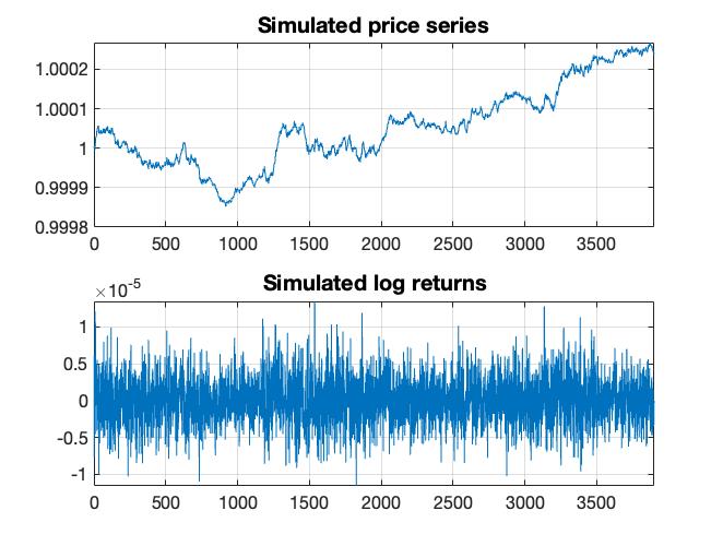
Figure 1: Simulated stock prices using the MJD dynamic given in Example 2.1 with six levels of the spot volatility $\sigma=\{2.12,1.51,2.35,1.83,2.44,1.65,3.13\}*10^{-4}$, $\mu=0.02$, $\nu=1$, $\mu_{J}=0.0$, $\sigma_{J}=0.015$. Top figure: Simulated stock price values. Bottom figure: Corresponding $\log$-returns, where the volatility regimes are visible with breakpoints at $780$, $1170$, $1950$, $3120$, and $3510$.

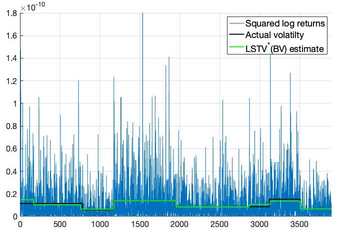
Figure 2: Comparison of LSTV^∗(BV) estimator fit for simulated stock prices with jumps and fixed levels of volatility for the stock prices simulated in Figure 1. Y-axis here is re-scaled $\sigma^{2}$.

Figure 2 displays the corresponding squared returns together with the comparison between the actual spot volatility and the estimated values using the LSTV^∗(BV) change points detection method with $K_{\mathrm{max}}=8$ and $\xi=0.03$. The estimator successfully detects all the breakpoints, providing a close fit with a small mean-square error between the true and estimated spot volatility. As for LSTV^∗(QV), it yields the same fit, and hence it is excluded from the plot.

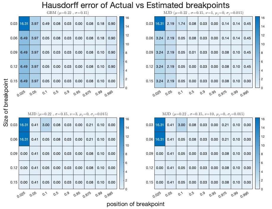
Figure 3: Hausdorff error comparison of LSTV^∗(BV) estimator fit for simulated stock prices with jumps and fixed levels of volatility with the position of jump size vs. changes in the size of jumps for different MJD models from Example 2.1. Top left: heat map is for classical Geometric Brownian Motion (MJD with no jumps) simulated stock prices of total sample size $3900$ with $\mu=0.22$ and various levels of sigma changes per row - $(\sigma_{1},\sigma_{2})$ are $(0.15,0.18)$, $(0.15,0.21)$, $(0.15,0.24)$, $(0.15,0.27)$, $(0.15,0.3)$, respectively. Each column indicates the position of the breakpoint in percentiles of actual data - $0.01$, $0.025$, $0.1$, $0.5$, $0.95$, $0.995$, $0.999$. Top right, bottom left, and bottom right: heat maps are MJD simulations with $\mu_{J}=0.0,\sigma_{J}=0.015$ and jump intensities $\nu=1,3,10$, respectively.

Next, to evaluate the numerical efficiency of the LSTV^∗ method, we perform a simulation with a single breakpoint at various positions and sizes within the simulated data. Our focus in this simulation is on locating the breakpoint rather than estimating the correct number of breakpoints. As such, we set $K_{\mathrm{max}}=1$ and keep $\xi=0.03$. We calculate the average Hausdorff distance over $10000$ random paths from the MJD model, using the same parameters as in the first simulation. To assess the robustness of our results, we set the jump intensity $\nu$ at four different levels, including the no-jumps case, as specified in the caption of Figure 3, and we vary the size of the change point and its position relative to the sample size as described in the $y$- and $x$-labels of Figure 3.

The results presented in Figure 3 demonstrate that the LSTV^∗(BV) method accurately estimates the true breakpoint, and is robust against varying jump intensity levels and change point locations. Across most simulations, the Hausdorff distance is less than $0.1\%$ of the observations, which corresponds to less than three observations, even when the change point is of the order of $0.03$ and located at the $0.995$ percentile of the sample (i.e., with only $20$ observations following the change point).

5.2 Estimation and Forecasting NYSE High Frequency Volatility

We evaluate the proposed estimators empirically using real financial data from the New York Stock Exchange (NYSE) for the period from January 2018 through June 2022. We select the ten largest stocks in terms of average market capitalization, based on data from NYSE Trade & Quote (TAQ). Because the trading times for the stocks are not synchronized, and prices are subject to market microstructure noise and end-of-day effects, we use mid-prices and impute missing values with neighboring prices. We obtain cleaned returns aggregated to frequencies of $1$, $5$, $15$, $30$, and $60$ minutes during trading hours between 9:30 a.m. and 4:00 p.m. The number of observations per day varies from 6 to 390, depending on the frequency. We do not include overnight returns, as they are influenced by external factors.

As an example, we present the $60$-minute frequency returns for Tesla (TSLA) from January 2018 to June 2022 in Figure 4. Using the LSTV^∗(BV) estimator with $K_{\mathrm{max}}=20$, we find that although there are many jumps in the returns, the algorithm detects only $\widehat{K}=5$ change points. Moreover, the persistent regimes in the volatility are only altered by major events related to the company or the market, as shown by the estimates of volatility.

If there are no change points, the LSTV(QV) and LSTV(BV) estimators reduce to the original $QV$ and $BV$ estimators, respectively. In the forecasting exercises below, we set $K_{\mathrm{max}}=1$ and $\xi=0.03$. We find that allowing for one change point improves forecasting performance across all models, assets, and frequencies considered below. We also experimented with $K_{\mathrm{max}}>1$, but the forecasting results were more mixed and sensitive to the choice of the $\xi>0$ parameter. In general, user should decide on the appropriate choice of $K_{\mathrm{max}}$ and $\xi$ based on past market and asset regime changes.

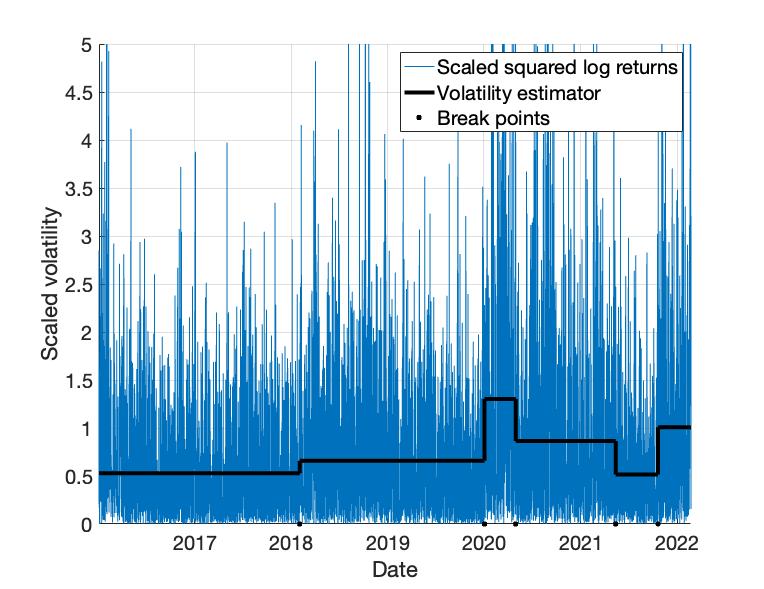
Figure 4: Tesla squared 60 minutes returns from January 2018 to August 2020 together with the estimated volatilities using LSTV^∗(BV) with $K_{\mathrm{max}}=20$. The estimator shows $5$ change points with different volatility regimes, especially from February 2020 to May 2020, i.e., during the early COVID-19 period.

To assess the forecasting ability of the proposed estimators, we compare them to various benchmarks. We conduct a rolling window exercise, in which we estimate our models and generate one-step-ahead forecasts for different frequencies of the data. Specifically, for a given window of data consisting of observations $r_{1,n},r_{2,n},\cdots,r_{t,n}$, we aim to forecast the spot volatility term at times $t+1$. The forecasts are calculated using the following formula

$$\sigma_{t\mid t+1,n}:=\mathbb{E}(\sigma\left((t+1)/n\right)|\{r_{s,n}\}_{s=1}^{t}).$$

To calculate the forecasts, we extrapolate the last estimated volatility $\widehat{\sigma}(t/n)$ obtained from the corresponding model within a given rolling window to $t+1$, for our high-frequency estimators. In the case of GARCH($1,1$) dynamics, we use the available explicit one-step-ahead GARCH($1,1$) forecast. We consider the entire historical data available in the rolling window to calculate the estimates, and no additional tuning parameters are required for the forecasting process.

As benchmark for the performance, we consider a broad spectrum of different volatility estimators that are commonly used in practice. Starting from the classical QV and BV estimators introduced by Barndorff-Nielsen and Shephard, (2004), we also include more recent refinements, such as the realized volatility and bipower variation (RVB) and realized volatility and quarticity (RVQ) estimators proposed by Yu, (2020). In addition, we consider the heavy-tailed $t$-GARCH model with Student-$t$ innovations, as well as its long-memory extension, the $t$-FIGARCH model, introduced by Shi and Ho, (2015). Finally, we include the mixed-frequency approach of the HAR model proposed by Corsi, (2009). However, the HAR model can only serve as a benchmark for multi-step (daily) volatility forecasts.

In Figure 5, we compare rolling window-based one-step-ahead forecasted volatilities and log forecasted volatilities of Apple’s 60-minute frequency returns using bipower variation, the $t$-GARCH(1,1), and LSTV^∗(BV) models. The forecasted volatilities for the BV model exhibit a large number of spikes across consecutive rolling windows, while the $t$-GARCH(1,1) produces forecasts with some extreme spikes. By contrast, our proposed model provides much smoother and more realistic forecasts, as can be seen from their autocorrelation structure. To further smooth the forecasts, we can use a simple exponential-moving average filter. The bottom plots in Figure 5 show the results of applying this filter, with the parameter $\lambda$ chosen to minimize the overall squared error.

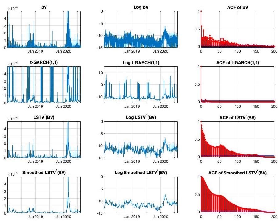
Figure 5: One-step-ahead forecasts from the rolling window exercise for the Apple 60 min stock using 2 weeks of the rolling window from January 2018 to August 2020. Row wise, a comparison between BV, $t$-GARCH(1,1), LSTV^∗(BV), and smoothed LSTV^∗(BV) models. First column: forecasted volatility values. Second column: log of the volatilities. Third column: autocorrelation functions of the forecasted volatilities.

To compare the forecast performance of different models quantitatively in our rolling window exercise, we use the prediction Average Squared Error (ASE) and the prediction Average Absolute Error (AAE), following the approach of Fryzlewicz et al., (2006),

$$ASE_{tp,2,N} =\frac{1}{N-tp-2}\sum_{t=2}^{N-fp}\left(\bar{\sigma}^{2}_{t+fp|t}-\bar{X}^{2}_{t+fp|t}\right)^{2}$$ (11)

$$AAE_{tp,2,N} =\frac{1}{N-tp-2}\sum_{t=2}^{N-fp}\left|\bar{\sigma}^{2}_{t+fp|t}-\bar{X}^{2}_{t+fp|t}\right|.$$ (12)

In the left panel of Figure 6, we compare the relative performance of GARCH(1,1) and our proposed method LSTV^∗(BV) to QV in terms of the percentage improvement in error. Our method shows a $10\%$ to $20\%$ improvement, while the $t$-GARCH(1,1) model exhibits a $30\%$ to $70\%$ worse performance than QV.

We extend our comparison analysis to include more recent log-memory variations of GARCH models. We use the FIGARCH model proposed by Shi and Ho, (2015) as a benchmark and introduce one more variation of our estimator by using the estimated volatility from LSTV^∗(QV) as innovations for the FIGARCH algorithm. This is referred to as LSTV^∗(FIGARCH). In Figure 6, we compare the relative performance of these three methods with respect to BV in terms of the percentage improvement in error. We find that both FIGARCH and LSTV^∗(FIGARCH) perform worse than the benchmark BV, while LSTV^∗(BV) outperforms all other methods across all frequencies of the data.

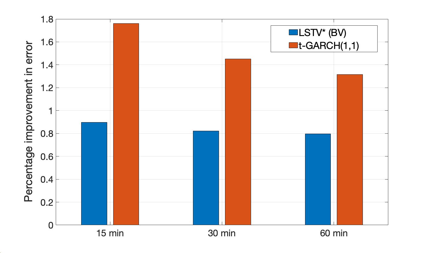
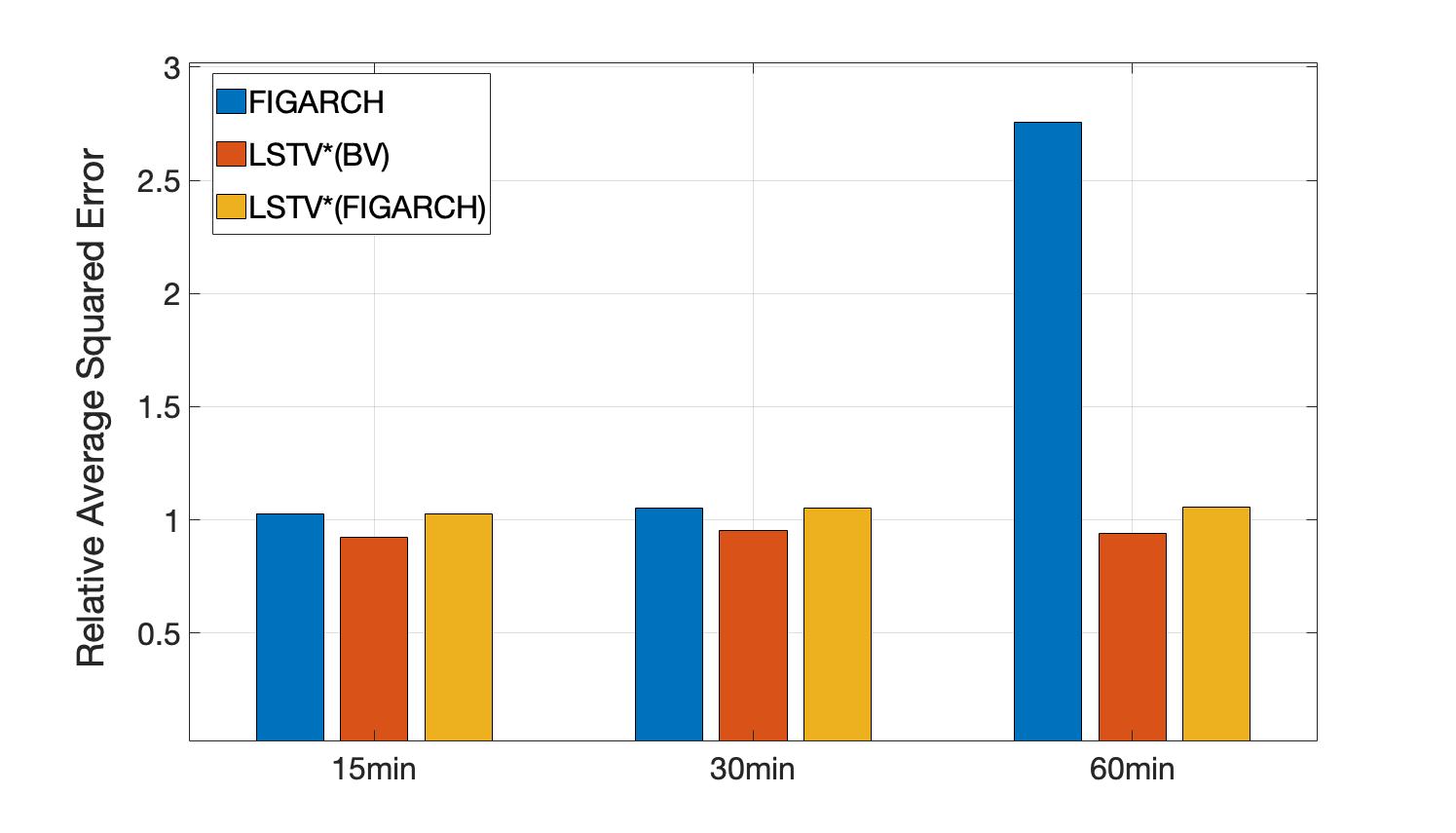
Figure 6: Percentage difference of one-step-ahead volatility forecasts in terms of predicted ASE from (11). Left Panel: LSTV^∗(BV) and $t$-GARCH(1,1) models relative to the QV model. Right Panel: FIGARCH, LSTV^∗(BV), and LSTV^∗(FIGARCH) models relative to the BV model.

In the following analysis, we compare the forecasting ability of our proposed method to the classical QV and BV estimators by Barndorff-Nielsen and Shephard, (2004), as well as the more recent refinements of them, including the realized volatility and bipower variation (RVB) and realized volatility and quarticity (RVQ) estimators proposed by Yu, (2020). In Figure 7, we present the Average Squared Error (ASE) of these estimators.

Our LSTV^∗(QV) method outperforms the underlying QV estimator, with a significant improvement observed across all frequencies. Furthermore, our LSTV^∗(BV) method also outperforms the standard BV estimator across all frequencies, which is a significant result in the context of one-step-ahead high-frequency volatility prediction.

The RVB and RVQ estimators are more efficient in terms of asymptotic variance, and thus exhibit better out-of-sample performance than QV, but still worse than BV and our LSTV^∗(BV).

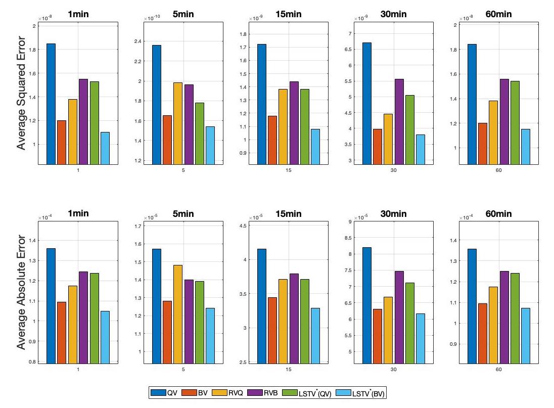
Figure 7: One-step-ahead volatility forecast errors for different volatility estimators (QV, BV, RVQ, RVB, LSTV^∗(QV), and LSTV^∗(BV)) and for different returns frequencies (1 min, 5 min, 15 min, 30 min, and 60 min). Top Panel: Average Squared Error (ASE) as in (11). Bottom Panel: Average Absolute Error(AAE) as in (12).

Daily volatility forecasts are more pragmatic and widely used in trading and portfolio optimization. Therefore, we also compare one-day-ahead volatility forecasts in Figure 8. In addition to the benchmarks used in Figure 7, we also include the HAR-RV method proposed by Corsi, (2009) in our comparison. Using a 2-week rolling window, we forecast the next-day volatility using different data frequencies. Our proposed method substantially outperforms all benchmarks, including the one generated by the HAR-RV model, in the one-day-ahead forecast.

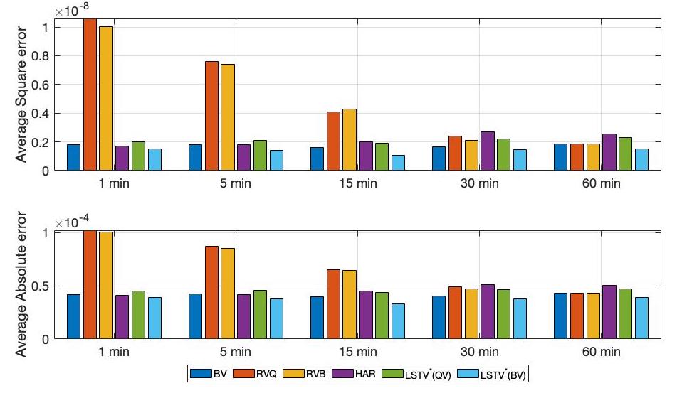
Figure 8: One-day-ahead volatility forecast errors for different volatility estimators (QV, BV, RVQ, RVB, LSTV^∗(QV), and LSTV^∗(BV)) and for different returns frequencies (1 min, 5 min, 15 min, 30 min, and 60 min). Top Panel: Average Squared Error (ASE) as in (11). Bottom Panel: Average Absolute Error(AAE) as in (12).

6 Extensions and Further Research

In addition to their performance in high-frequency volatility estimation, our proposed volatility estimators can be extended to capture other stylized facts of high-frequency volatility, demonstrating their versatility and practical applicability. For example, one can filter jumps from the stock prices separately from the volatility estimation by adding an additional $\ell_{1}$ regularization term to the objective function in (7).

Similarly, intraday or weekly seasonality, a well-known statistical characteristic of high-frequency stock volatility, can be incorporated into our $\ell_{1}$ volatility filter. One approach for incorporating seasonality is to follow Vatter et al., (2015) and incorporate smooth trend and seasonality into the framework. To capture both effects, the objective function (7) can be modified as follows:

$$\dfrac{1}{n}\left\lVert F(\mathbf{r}_{t})-\mathbf{X}\boldsymbol{\beta}-\mathbf{s}-\mathbf{v}\right\rVert^{2}_{2}+\lambda\left\lVert\boldsymbol{\beta}\right\rVert_{1}+\gamma\left\lVert\mathbf{v}\right\rVert_{1}$$

$$\textrm{s.t.}\quad s_{t+p}=s_{t}\quad t=1,\ldots,n-p,$$

where $\mathbf{s}=(s_{1},\ldots,s_{n})^{\prime}\in\mathbb{R}^{n}$ is the seasonal periodic component with known period $p$, vector $\mathbf{v}\in\mathbb{R}^{n}$ is the sparse spikes component, and the parameter $\gamma\geq 0$ controls jumps intensity.

If the exact seasonality pattern needs to be estimated from the data one can use

$$\dfrac{1}{n}\left\lVert F(\mathbf{r}_{t})-\mathbf{X}\boldsymbol{\beta}-\mathbf{s}-\mathbf{v}\right\rVert^{2}_{2}+\lambda\left\lVert\boldsymbol{\beta}\right\rVert_{1}+\gamma\left\lVert\mathbf{v}\right\rVert_{1}$$

$$\quad\quad\quad\quad\quad\ \quad\quad\quad\quad\quad\quad+\sum_{\omega\in\Omega}\left(\left|a_{\omega}\right|+\left|b_{\omega}\right|\right)$$

$$\textrm{s.t.}\quad s_{t}=\sum_{\omega\in\Omega}a_{\omega}\sin(\omega t)+b_{\omega}\cos(\omega t)\quad t=1,\ldots,n.$$

The $\mathbf{s}=(s_{1},\ldots,s_{n})^{\prime}\in\mathbb{R}^{n}$ filter is responsible for selecting the best frequencies from an over-complete dictionary $\Omega$. In this case, the frequency does not need to be known a priori, and the penalty term discourages the use of the dictionary in a greedy way. For an adaptive version of this filter and a fast coordinate descent algorithm for estimation, see Souto et al., (2016).

Secondly, one of the assumptions in our analysis so far is that the stock returns are equally spaced because the data used in Section 5 consists of TAQ data aggregated to 1, 5, 10, 30, and 60-minute intervals. We can extend our method to tick-level data, which is irregularly spaced. First, consider the estimation of the underlying continuous volatility from a finite number of data points. Equation (7) can be extended to a continuous form as follows:

$$\dfrac{1}{n}\sum_{i=1}^{n}(F(\mathbf{r}_{t})_{i}-x_{i})^{2}+\lambda\int_{t_{1}}^{t_{n}}\left\lvert\dot{x}\right\rvert\mbox{d}t.$$

This can be simplified by using the standard interpolation problem as explained in Kim et al., (2009). In particular, we can solve

$$\dfrac{1}{n}\sum_{i=1}^{n}\left(F(\mathbf{r}_{t})_{t_{i}}-x_{t_{i}}\right)^{2}+\lambda\sum_{i=2}^{n}\left\lvert\frac{x_{t_{i+1}}-x_{t_{i}}}{t_{i+1}-t_{i}}\right\rvert.$$ (13)

Using the optimal points $x_{t_{i}}$, $i=1,\ldots,n$, we can recover the solution to the original piecewise linear trend filtering problem: the piecewise-linear function, $x^{*}_{t}$, for $x^{*}_{t_{i}}$, given by

$$x^{*}_{t}=\frac{t_{i+1}-t}{t_{i+1}-t_{i}}x^{*}_{i},$$

where $i=1,\ldots,n$, is the optimal piecewise constant volatility. To reflect the non-equally spaced data, one can modify the proposed LSTV^∗ algorithm by modifying the matrix $\mathbf{X}$ to include the time increments from the regularization term. Alternatively, one can use the modified version of the primal-dual algorithm described in Kim et al., (2009).

In this paper, we assumed that the observed returns are the true returns. In ultra-high-frequency data, one needs to accommodate the assumption of microstructure noise. We can do that by using a realized kernel estimator $F_{\mathfrak{K}}(\mathbf{r}_{t})$, where $\mathfrak{K}$ stands for the specific kernel function (see Barndorff-Nielsen et al., , 2008; Barndorff-Nielsen et al., , 2009; Barndorff-Nielsen et al., 2011a, ; Barndorff-Nielsen et al., 2011b, , and Lunde et al., , 2015). Indeed, if we have

$$p(t)=p^{*}(t)+\epsilon(t),$$

where $p(t)$ denotes the observed price at $t$, $p^{*}(t)$ denotes the true price at $t$, and $\epsilon$ denotes the micro-structure noise; then the returns satisfy

$$r_{t}=r^{*}_{t}+u_{t},$$

where $u_{t}=\epsilon(t)-\epsilon(t-1)$, and one can construct a kernel-based estimator $F_{\mathfrak{K}}$ that satisfies

$$\operatorname*{\mathit{p}-\lim}_{n\rightarrow+\infty}F_{\mathfrak{K}}(\mathbf{r}_{t})=[\mathbf{r}^{*}_{t}]\text{ and }\operatorname*{\mathit{p}-\lim}_{n\rightarrow+\infty}=F_{\mathfrak{K}}(\mathbf{u}_{t})=0,$$

where $\mathbf{r}_{t}$ is the vector of high frequency returns; as before, $[\mathbf{r}^{*}_{t}]$ is the quadratic variation of the true returns; and $\mathbf{u}_{t}=(u_{1},\cdots,u_{n})$.

Finally, the two estimators proposed in this paper allow constructing an estimator of the jump component. Namely, one can take the differences between increments of the QV and BV estimator and plug them into the objective function with $\ell_{1}$ regularization not on the difference but on the series itself, i.e.,

$$\widehat{\mathbf{u}}(\lambda) :=\operatorname*{argmin}_{\mathbf{u}\in\mathbb{R}^{n-1}}\mathcal{L}(\mathbf{u})$$ (14)

$$\mbox{where }\mathcal{L}(\mathbf{u}) :=\frac{1}{n}\left\lVert\tilde{F}_{\text{RV}}(\mathbf{r}_{t})-F_{\text{BP}}(\mathbf{r}_{t})-\mathbf{u}\right\rVert^{2}_{2}+\lambda\left\lVert\mathbf{u}\right\rVert_{1},$$

where $\tilde{F}_{\text{RV}}$ is the original ${F}_{\text{RV}}$ with the first element $r_{1,t}^{2}$ in the vector removed. The $\widehat{\mathbf{u}}(\lambda)$ in (14) estimates the jump component of the price process. They can be obtained via the original LARS or any other LASSO related algorithm. Since $\tilde{F}_{\text{RV}}(\mathbf{r}_{t})-F_{\text{BP}}(\mathbf{r}_{t})$ satisfies our consistency condition for the jump component, the results in this paper also show that $\widehat{\mathbf{u}}(\lambda)$ will be consistent for the true jump sizes and their locations.

7 Conclusions

In this paper, we have introduced a new family of high-frequency volatility estimators. By leveraging the LSTV change point detection framework and adding $\ell_{1}$ regularization to two classical estimators (quadratic variation and bipower variation), we have proposed estimators that are consistent for volatility estimation and breakpoint detection. Simulation results demonstrate that the proposed estimators accurately identify breakpoints and outperform classical and recent high-frequency volatility estimators in terms of out-of-sample volatility prediction at all frequencies and forecasting horizons.

Our proposed estimators offer practical advantages, such as their ability to accurately identify breakpoints close to the end of the sample and their ability to provide more realistic and smoother volatility forecasts. In future research, we plan to extend the proposed estimators to the multivariate case and incorporate other stylized facts of (ultra) high-frequency financial returns using the extensions discussed in Section 6.

Overall, our proposed estimators have significant potential for improving high-frequency volatility estimation and forecasting. We hope that our work will inspire further research in this area and lead to practical applications in electronic trading, portfolio optimization, and risk management.

Appendix A Sub-Weibull random variables

A random variable $X$ with sub-Weibull distribution with tail parameter $\alpha$ is one such that

$$\forall t>0:\mathbb{P}\left(\left\lvert X-\mathbb{E}[X]\right\rvert\geq t\right)\leq 2\exp\left(-(t/C)^{\alpha}\right)$$

for some $\alpha,C>0$. Particularly, the parameters $\alpha=1$ and $\alpha=2$ correspond to sub-exponential and sub-Gaussian random variables, respectively. This class of heavy-tailed distributions (and a corresponding notion for random vectors) has recently been defined and studied in (Kuchibhotla and Chakrabortty, , 2022). (See also Zhang and Wei, , 2022.) Concentration inequalities for such random variables (and the corresponding random vectors) have also been recently derived in (Götze et al., , 2021) and (Sambale, , 2020). Many of these results have been extended to a larger class of heavy-tailed distributions in (Bakhshizadeh et al., , 2020).

We recall a couple of properties of sub-Weibull distributions. Note that an equivalent definition of the class $\mathrm{subWeib}(\alpha)$ can be stated in terms of Orlicz-(quasi-)norms. Indeed, $X\in\mathrm{subWeib}(\alpha)$ if and only if

$$\left\lVert X\right\rVert_{\Psi_{\alpha}}:=\inf\left\{\eta>0:\mathbb{E}\left[\exp\left(\left(X/\eta\right)^{\alpha}\right)\right]\leq 2\right\}$$

is finite. Here, $\Psi_{\alpha}$ denotes the Orlicz function $s\mapsto\exp(s^{\alpha})-1$, $\alpha>0$.

Note that in general, the constant $C$ in the tail bound definition of a sub-Weibull random variable $X$ and $\left\lVert X\right\rVert_{\Psi_{\alpha}}$ are proportional to each other by a positive factor depending only on $\alpha$. (See (Sambale, , 2020) and (Götze et al., , 2021).)

Proposition A.1.

(Vladimirova et al., , 2020, Proposition 2.3) Let $X_{1}$ and $X_{2}$ be sub-Weibull random variables with tail parameters $\alpha_{1}$ and $\alpha_{2}$, respectively. Then, $X_{1}X_{2}$ and $X_{1}+X_{2}$ are sub-Weibull with respective tail parameters $\alpha_{1}+\alpha_{2}$ and $\max(\alpha_{1},\alpha_{2})$.

Proposition A.2.

Let the random variables $X_{1},\cdots,X_{n}\in\mathrm{subWeib}(\alpha)$, with $\alpha>0$, be independent, and suppose that $\left\lVert X_{i}\right\rVert_{\Psi_{\alpha}}\leq M$ for all $i=1,\cdots,n$. Then, for all $n\geq 1$ and $t>0$, we have

$$\mathbb{P}\left(\dfrac{1}{n}\left\lvert\sum_{i=1}^{n}\left(X_{i}-\mathbb{E}(X_{i})\right)\right\rvert\geq t\right)\leq 2\exp\left(-\dfrac{1}{C_{\alpha}}\cdot\dfrac{t^{\alpha}n^{\alpha/2}}{M^{\alpha}}\right)$$

where $C_{\alpha}>0$ is a universal constant depending only on $\alpha$.

This follows from the proof of (Sambale, , 2020, Lemma 5.2).

As a contribution to this existing literature, we prove the following result on random sums of sub-Weibull random variables.

Proposition A.3.

Let $Z_{1},Z_{2},\cdots$ be a sequence of i.i.d. sub-Weibull random variables with decay parameter $\alpha>0$ and common sub-Weibull norm $\left\lVert Z\right\rVert_{\Psi_{\alpha}}$, with $Z$ denoting the common distribution of the $Z_{j}$’s. Suppose in addition that $W$ is independent of the $Z_{j}$’s. Then the sum $\sum_{j=1}^{W}Z_{j}$ is also sub-Weibull with decay parameter $\alpha$ and sub-Weibull norm $\mathbb{E}\left(W^{1+A(\alpha)}\right)\left\lVert Z\right\rVert_{\Psi_{\alpha}}$ for some $A(\alpha)$ such that $-\max\left\{1,1/\alpha\right\}\leq A(\alpha)\leq 1/\alpha+\left\lvert 1-1/\alpha\right\rvert$.

Proof.

By the law of total expectation, we have:

$$\left\lVert\sum_{j=1}^{W}Z_{j}\right\rVert_{\Psi_{\alpha}}=\mathbb{E}\left(\left\lVert\sum_{j=1}^{W}Z_{j}\right\rVert_{\Psi_{\alpha}}\right)=\mathbb{E}\left(\mathbb{E}\left(\left\lVert\sum_{j=1}^{W}Z_{j}\right\rVert_{\Psi_{\alpha}}\Bigg{|}W\right)\right).$$

Now, in order to compute $\mathbb{E}\left(\left\lVert\sum_{j=1}^{W}Z_{j}\right\rVert_{\Psi_{\alpha}}\Bigg{|}W\right)$, we compute the sub-Weibull norm of a deterministic sum of sub-Weibull random variables.

By the concavity of $x\mapsto\left\lvert x\right\rvert^{\alpha}$ for $\alpha\in(0,1)$ and its convexity for $\alpha\geq 1$, we have the following for any $a_{1},\cdots,a_{m}\geq 0$:

$$\min\left\{1,m^{\alpha-1}\right\}\sum_{j=1}^{m}a_{j}^{\alpha}\leq\left(\sum_{j=1}^{m}a_{j}\right)^{\alpha}\leq\max\left\{1,m^{\alpha-1}\right\}\sum_{j=1}^{m}a_{j}^{\alpha}.$$

On the one hand,

$$\mathbb{E}\left[\exp\left(\dfrac{\left\lvert\sum_{j=1}^{m}Z_{j}\right\rvert^{\alpha}}{m\cdot\dfrac{\max\left\{1,m^{\alpha-1}\right\}}{\min\left\{1,m^{\alpha-1}\right\}}\left(\sum_{j=1}^{m}\left\lVert Z_{j}\right\rVert_{\Psi_{\alpha}}\right)^{\alpha}}\right)\right] \leq\mathbb{E}\left[\exp\left(\dfrac{\max\left\{1,m^{\alpha-1}\right\}\sum_{j=1}^{m}\left\lvert Z_{j}\right\rvert^{\alpha}}{m\cdot\max\left\{1,m^{\alpha-1}\right\}\sum_{j=1}^{m}\left\lVert Z_{j}\right\rVert^{\alpha}_{\Psi_{\alpha}}}\right)\right]$$

$$\leq\mathbb{E}\left[\left(\prod_{j=1}^{m}\left(\exp\left(\dfrac{\left\lvert Z_{j}\right\rvert^{\alpha}}{\left\lVert Z_{j}\right\rVert^{\alpha}_{\Psi_{\alpha}}}\right)\right)^{1/m}\right)\right]$$

$$\leq\mathbb{E}\left(\dfrac{1}{m}\sum_{j=1}^{m}\exp\left(\dfrac{\left\lvert Z_{j}\right\rvert^{\alpha}}{\left\lVert Z_{j}\right\rVert^{\alpha}_{\Psi_{\alpha}}}\right)\right)$$

$$=\dfrac{1}{m}\mathbb{E}\left(\exp\left(\dfrac{\left\lvert Z_{j}\right\rvert^{\alpha}}{\left\lVert Z_{j}\right\rVert^{\alpha}_{\Psi_{\alpha}}}\right)\right)=\dfrac{1}{m}\cdot(2\cdot m)=2.$$

The third inequality follows from the AM-GM inequality while the next step follows from the definition of the sub-Weibull norm. Therefore,

$$\left\lVert\sum_{j=1}^{m}Z_{j}\right\rVert_{\Psi_{\alpha}}\leq\left(m\cdot\dfrac{\max\left\{1,m^{\alpha-1}\right\}}{\min\left\{1,m^{\alpha-1}\right\}}\right)^{1/\alpha}\sum_{j=1}^{m}\left\lVert Z_{j}\right\rVert_{\Psi_{\alpha}}.$$

On the other hand,

$$\mathbb{E}\left[\exp\left(\dfrac{\left\lvert Z_{j}\right\rvert^{\alpha}}{\dfrac{1}{\min\left\{1,m^{\alpha-1}\right\}}\left\lVert\sum_{j=1}^{m}Z_{j}\right\rVert^{\alpha}_{\Psi_{\alpha}}}\right)\right] \leq\mathbb{E}\left[\exp\left(\dfrac{\dfrac{1}{\min\left\{1,m^{\alpha-1}\right\}}\left\lvert\sum_{j=1}^{m}Z_{j}\right\rvert^{\alpha}}{\dfrac{1}{\min\left\{1,m^{\alpha-1}\right\}}\left\lVert\sum_{j=1}^{m}Z_{j}\right\rVert^{\alpha}_{\Psi_{\alpha}}}\right)\right]$$

$$=\mathbb{E}\left[\exp\left(\dfrac{\left\lvert\sum_{j=1}^{m}Z_{j}\right\rvert^{\alpha}}{\left\lVert\sum_{j=1}^{m}Z_{j}\right\rVert^{\alpha}_{\Psi_{\alpha}}}\right)\right]\leq 2.$$

Therefore, for each $j=1,\cdots,m$,

$$\left\lVert Z_{j}\right\rVert_{\Psi_{\alpha}}\leq\left(\dfrac{1}{\min\left\{1,m^{\alpha-1}\right\}}\right)^{1/\alpha}\left\lVert\sum_{j=1}^{m}Z_{j}\right\rVert_{\Psi_{\alpha}},$$

so that

$$\left(\dfrac{\min\left\{1,m^{\alpha-1}\right\}}{m^{\alpha}}\right)^{1/\alpha}\sum_{j=1}^{m}\left\lVert Z_{j}\right\rVert_{\Psi_{\alpha}}\leq\left\lVert\sum_{j=1}^{m}Z_{j}\right\rVert_{\Psi_{\alpha}}.$$

In conclusion,

$$m^{-\max\{1,1/\alpha\}}\sum_{j=1}^{m}\left\lVert Z_{j}\right\rVert_{\Psi_{\alpha}}\leq\left\lVert\sum_{j=1}^{m}Z_{j}\right\rVert_{\Psi_{\alpha}}\leq m^{1/\alpha+\left\lvert 1-1/\alpha\right\rvert}\sum_{j=1}^{m}\left\lVert Z_{j}\right\rVert_{\Psi_{\alpha}}.$$

Therefore,

$$\left\lVert\sum_{j=1}^{m}Z_{j}\right\rVert_{\Psi_{\alpha}}=m^{A(\alpha)}\sum_{j=1}^{m}\left\lVert Z_{j}\right\rVert_{\Psi_{\alpha}},$$

for some exponent $A(\alpha)$ such that $-\max\left\{1,1/\alpha\right\}\leq A(\alpha)\leq 1/\alpha+\left\lvert 1-1/\alpha\right\rvert$.

The latter implies that

$$\mathbb{E}\left(\left\lVert\sum_{j=1}^{W}Z_{j}\right\rVert_{\Psi_{\alpha}}\Bigg{|}W\right)=\mathbb{E}\left(W^{A(\alpha)}\sum_{j=1}^{W}\left\lVert Z_{j}\right\rVert_{\Psi_{\alpha}}\Bigg{|}W\right)=\mathbb{E}\left(W^{A(\alpha)}W\left\lVert Z\right\rVert_{\Psi_{\alpha}}\right)=\mathbb{E}\left(W^{1+A(\alpha)}\right)\left\lVert Z\right\rVert_{\Psi_{\alpha}}.$$

Ultimately, we conclude that $\sum_{j=1}^{W}Z_{j}$ is sub-Weibull with decay parameter $\alpha$ with sub-Weibull norm $\mathbb{E}\left(W^{1+A(\alpha)}\right)\left\lVert Z\right\rVert_{\Psi_{\alpha}}$. ∎

Appendix B Technical Lemmas

Lemma B.1.

Let $\left(\widehat{t}_{1},\cdots,\widehat{t}_{n}\right)$ denote the change point estimates defined in 10. Then $\left(\widehat{t}_{1},\cdots,\widehat{t}_{n}\right)$ and $\left(\widehat{u}_{1},\cdots,\widehat{u}_{n}\right)$ satisfy

$$\forall\ell\in\left\{1,\cdots,\left\lvert\widehat{\mathcal{A}}(\lambda)\right\rvert\right\}:\sum_{i=\widehat{t}_{\ell}}^{n}F(\mathbf{r}_{t})_{i}-\sum_{i=\widehat{t}_{\ell}}^{n}\widehat{u}_{i}=\dfrac{n\lambda}{2}\mathrm{sign}\left(\widehat{u}_{\widehat{t}_{\ell}(\lambda)}-\widehat{u}_{\widehat{t}_{\ell}(\lambda)-1}\right),\text{ and }$$ (15)

$$\forall j\in\left\{1,\cdots,n\right\}:\left\lvert\sum_{i=j}^{n}F(\mathbf{r}_{t})_{i}-\sum_{i=j}^{n}\widehat{u}_{i}\right\rvert\leq\dfrac{n\lambda}{2}.$$ (16)

The vector $\left(\widehat{u}_{1}(\lambda),\cdots,\widehat{u}_{n}(\lambda)\right)$ satisfies:

$$\widehat{u}_{j}(\lambda)=\widehat{\eta}_{k}\text{ for }\widehat{t}_{k-1}(\lambda)\leq j\leq\widehat{t}_{k}(\lambda)-1,$$ (17)

for some constant values $\widehat{\eta}_{1},\cdots,\widehat{\eta}_{\widehat{K}}$, where $\widehat{K}\geq 1$.

For a proof, see (Harchaoui and Lévy-Leduc, , 2010). The proof simply relies on a minimization criterion based on sub-gradients for each one of the objective functions.

In what follows, let $\mathbf{Z}[r,s]:=\sum_{i=r}^{s}Z_{i}$ for any random vector $\mathbf{Z}=(Z_{1},\cdots,Z_{n})$.

Lemma B.2.

Let $\varepsilon_{J,1,t},\cdots,\varepsilon_{J,n,t}$ be $\mathrm{subWeib}(\alpha)$ jump-corruption variables previously defined. If $\{\zeta_{n}\}_{n\geq 1}$ and $\{\mu_{n}\}_{n\geq 1}$ are two positive sequences such that $\mu^{\alpha}_{n}\zeta_{n}^{\alpha}\left[\log(n)\right]^{-1}\xrightarrow[n\to+\infty]{}+\infty$, then

$$\mathbb{P}\left(\sup_{\begin{subarray}{c}1\leq r_{n}<s_{n}\leq n\\ \left\lvert r_{n}-s_{n}\right\rvert\geq\zeta_{n}\end{subarray}}\left\lvert\dfrac{\mathfrak{E}_{J,t}[r_{n},s_{n}-1]}{s_{n}-r_{n}}\right\rvert\geq\mu_{n}\right)\xrightarrow[n\to+\infty]{}0.$$

Proof.

Clearly,

$$\mathbb{P}\left(\sup_{\begin{subarray}{c}1\leq r_{n}<s_{n}\leq n\\ \left\lvert r_{n}-s_{n}\right\rvert\geq\zeta_{n}\end{subarray}}\left\lvert\dfrac{\mathfrak{E}_{J,t}[r_{n},s_{n}-1]}{s_{n}-r_{n}}\right\rvert\geq\mu_{n}\right)\leq\sum_{\begin{subarray}{c}1\leq r_{n}<s_{n}\leq n\\ \left\lvert r_{n}-s_{n}\right\rvert\geq\zeta_{n}\end{subarray}}\mathbb{P}\left(\left\lvert\dfrac{\mathfrak{E}_{J,t}[r_{n},s_{n}-1]}{s_{n}-r_{n}}\right\rvert\geq\mu_{n}\right).$$

By Proposition A.3, we have:

$$\mathbb{P}\left(\left\lvert\dfrac{\mathfrak{E}_{J,t}[r_{n},s_{n}-1]}{s_{n}-r_{n}}\right\rvert\geq\mu_{n}\right) =\mathbb{P}\left(\left\lvert\sum_{i=r_{n}}^{s_{n}-1}\varepsilon_{J,i,t}\right\rvert\geq\mu_{n}\left\lvert s_{n}-r_{n}\right\rvert\right),$$

$$=\chi_{J}(1-\chi_{R})\mathbb{P}\left(\left\lvert\sum_{j=\mathfrak{X}_{\tau_{r_{n}-1,t}}+1}^{\mathfrak{X}_{\tau_{s_{n}-1,t}}}Q^{2}_{j}\right\rvert\geq\mu_{n}\left\lvert s_{n}-r_{n}\right\rvert\right)$$

$$=\chi_{J}(1-\chi_{R})\mathbb{P}\left(\left\lvert\sum_{j=1}^{\mathfrak{X}_{\tau_{s_{n}-1,t}}}Q^{2}_{j}-\sum_{j=1}^{\mathfrak{X}_{\tau_{r_{n}-1,t}}}Q^{2}_{j}\right\rvert\geq\mu_{n}\left\lvert s_{n}-r_{n}\right\rvert\right)$$

$$\leq\chi_{J}(1-\chi_{R})\mathbb{P}\left(\left\lvert\sum_{j=1}^{\mathfrak{X}_{\tau_{s_{n}-1,t}}}Q^{2}_{j}\right\rvert\geq\dfrac{1}{2}\mu_{n}\left\lvert s_{n}-r_{n}\right\rvert\right)$$

$$\quad+\chi_{J}(1-\chi_{R})\mathbb{P}\left(\left\lvert\sum_{j=1}^{\mathfrak{X}_{\tau_{r_{n}-1,t}}}Q^{2}_{j}\right\rvert\geq\dfrac{1}{2}\mu_{n}\left\lvert s_{n}-r_{n}\right\rvert\right)$$

$$\leq 4\chi_{J}(1-\chi_{R})\exp\left(-\dfrac{\mu_{n}^{\alpha}\left\lvert s_{n}-r_{n}\right\rvert^{\alpha}}{\mathbb{E}\left[\mathfrak{X}_{t}^{1+A(\alpha/2)}\right]^{\alpha/2}\left\lVert Q\right\rVert^{\alpha}_{\Psi_{\alpha}}}\right),$$

where $C$ is the constant defined in Proposition A.3. Summing over $1<r_{n}<s_{n}\leq n$ with $\left\lvert r_{n}-s_{n}\right\rvert\geq\zeta_{n}$, we obtain

$$\mathbb{P}\left(\sup_{\begin{subarray}{c}1\leq r_{n}<s_{n}\leq n\\ \left\lvert r_{n}-s_{n}\right\rvert\geq\zeta_{n}\end{subarray}}\left\lvert\dfrac{\mathfrak{E}_{J,t}[r_{n},s_{n}-1]}{s_{n}-r_{n}}\right\rvert\geq\mu_{n}\right) \leq 4\left(\dfrac{n(n-1)}{2}\right)\exp\left(-\dfrac{\mu_{n}^{\alpha}\zeta^{\alpha}_{n}}{\mathbb{E}\left[\mathfrak{X}_{t}^{1+A(\alpha/2)}\right]^{\alpha/2}\left\lVert Q\right\rVert^{\alpha}_{\Psi_{\alpha}}}\right)$$

$$\leq 2\exp\left[2\log(n)\left(1-\dfrac{1}{\mathbb{E}\left[\mathfrak{X}_{t}^{1+A(\alpha/2)}\right]^{\alpha/2}\left\lVert Q\right\rVert^{\alpha}_{\Psi_{\alpha}}}\cdot\dfrac{\mu^{\alpha}_{n}\zeta_{n}^{\alpha}}{\log(n)}\right)\right],$$

and the latter upper bound converges to $0$ as $\mu^{\alpha}_{n}\zeta_{n}^{\alpha}\left[\log(n)\right]^{-1}\xrightarrow[n\to+\infty]{}+\infty$. ∎

Appendix C Proofs of the Results

In this section, we present the proofs of the results outlined in the paper.

Proof of Proposition 2.2.

The consistency condition (4) implies

$$\operatorname*{\mathit{p}-\lim}_{n\rightarrow+\infty}\left(\sum_{i=1}^{n}(F(\mathbf{r}_{t})_{i}-y_{t,i})\right)^{2}=0,$$

which in turn implies

$$\operatorname*{\mathit{p}-\lim}_{n\to+\infty}\dfrac{1}{n}\sum_{k=1}^{n}\left\lvert\sum_{i=1}^{k}(F(\mathbf{r}_{t})_{i}-y_{t,i})\right\rvert^{2}=0.$$

In particular, denoting $\Delta_{i}:=F(\mathbf{r}_{t})_{i}-y_{t,i}$ and $S_{i}:=\left\lvert\sum_{k=1}^{i}\Delta_{k}\right\rvert^{2}$, we write:

$$\operatorname*{\mathit{p}-\lim}_{n\rightarrow+\infty}\dfrac{1}{n}\sum_{i=1}^{n}S_{i}=0.$$

Using this, we can show that our estimator is consistent with respect mean squared error. First, let us expand the sum of squares:

$$\sum_{i=1}^{n}\Delta^{2}_{i}=\left(\sum_{i=1}^{n}\Delta_{i}\right)^{2}-\sum_{1\leq k<i\leq n}2\Delta_{i}\Delta_{k}.$$

Second, using Young’s inequality, we can bound the sum of products in the following manner, for any $\gamma>0$:

$$\left\lvert\sum_{1\leq k<i\leq n}2\Delta_{i}\Delta_{k}\right\rvert=\left\lvert\sum_{i=1}^{n}\sum_{k=1}^{i-1}2\Delta_{i}\Delta_{k}\right\rvert=\left\lvert\sum_{i=1}^{n}2\Delta_{i}\left(\sum_{k=1}^{i-1}\Delta_{k}\right)\right\rvert \leq\sum_{i=1}^{n}\left\lvert 2\Delta_{i}\left(\sum_{k=1}^{i-1}\Delta_{k}\right)\right\rvert$$

$$\leq\sum_{i=1}^{n}\left[\gamma\Delta^{2}_{i}+\dfrac{1}{\gamma}\left(\sum_{k=1}^{i-1}\Delta_{k}\right)^{2}\right].$$

Therefore, for any $\gamma\in(0,1)$ in particular, we have:

$$\sum_{i=1}^{n}\Delta^{2}_{i}\leq S_{n}+\gamma\sum_{i=1}^{n}\Delta^{2}_{i}+\dfrac{1}{\gamma}\sum_{i=0}^{n-1}S_{i}.$$

But since $S_{0}=0$ and $1/\gamma>1$, it follows that

$$(1-\gamma)\sum_{i=1}^{n}\Delta^{2}_{i}\leq\dfrac{1}{\gamma}\sum_{i=1}^{n}S_{i},$$

and so after dividing by $1-\gamma$ and minimizing over $\gamma$, we conclude that

$$\dfrac{1}{n}\sum_{i=1}^{n}\Delta^{2}_{i}\leq 4\left(\dfrac{1}{n}\sum_{i=1}^{n}S_{i}\right).$$

It thus follows that

$$\operatorname*{\mathit{p}-\lim}_{n\rightarrow+\infty}\left(\dfrac{1}{n}\sum_{i=1}^{n}(F(\mathbf{r}_{t})_{i}-y_{t,i})^{2}\right)=0.$$

∎

Proof of Proposition 4.1.

By the definition of $\widehat{\boldsymbol{\beta}}$,

$$\dfrac{1}{n}\left\lVert F(\mathbf{r}_{t})-\mathbf{X}\widehat{\boldsymbol{\beta}}\right\rVert^{2}_{2}+\lambda\left\lVert\widehat{\boldsymbol{\beta}}\right\rVert_{1}\leq\dfrac{1}{n}\left\lVert F(\mathbf{r}_{t})-\mathbf{X}\boldsymbol{\beta}^{*}_{\sigma}\right\rVert^{2}_{2}+\lambda\left\lVert\boldsymbol{\beta}^{*}_{\sigma}\right\rVert_{1}.$$

We thus have:

$$\dfrac{1}{n}\left\lVert\mathbf{X}\left(\widehat{\boldsymbol{\beta}}-\boldsymbol{\beta}^{*}_{\sigma}\right)\right\rVert^{2}_{2}+\dfrac{2}{n}\left\langle F(\mathbf{r}_{t})-\mathbf{X}\boldsymbol{\beta}^{*}_{\sigma},\mathbf{X}\left(\widehat{\boldsymbol{\beta}}-\boldsymbol{\beta}^{*}_{\sigma}\right)\right\rangle_{2}\leq\lambda\left(\left\lVert\boldsymbol{\beta}^{*}_{\sigma}\right\rVert_{1}-\left\lVert\widehat{\boldsymbol{\beta}}\right\rVert_{1}\right).$$

Using the fact that $\left\lVert\cdot\right\rVert_{1}\leq\sqrt{n}\left\lVert\cdot\right\rVert_{2}$, Young’s inequality, we see that for any $\gamma>0$,

$$(1-\gamma)\left(\dfrac{1}{n}\left\lVert\mathbf{X}\left(\widehat{\boldsymbol{\beta}}-\boldsymbol{\beta}^{*}_{\sigma}\right)\right\rVert^{2}_{2}\right)-\dfrac{1}{\gamma}\left(\dfrac{1}{n}\left\lVert F(\mathbf{r}_{t})-\mathbf{X}\boldsymbol{\beta}^{*}_{\sigma}\right\rVert^{2}_{2}\right)\leq\lambda\sqrt{n}\left\lVert\mathbf{X}\left(\widehat{\boldsymbol{\beta}}-\boldsymbol{\beta}^{*}_{\sigma}\right)\right\rVert_{2}.$$

Using Young’s inequality again, we obtain that for any $\kappa>0$,

$$(1-\gamma-\kappa)\left(\dfrac{1}{n}\left\lVert\mathbf{X}\left(\widehat{\boldsymbol{\beta}}-\boldsymbol{\beta}^{*}_{\sigma}\right)\right\rVert^{2}_{2}\right)\leq\dfrac{1}{\gamma}\left(\dfrac{1}{n}\left\lVert F(\mathbf{r}_{t})-\mathbf{X}\boldsymbol{\beta}^{*}_{\sigma}\right\rVert^{2}_{2}\right)+\dfrac{1}{\kappa}\lambda^{2}n^{2}.$$

Using the Cauchy-Schwarz inequality, and using the fact that $\left\lVert\cdot\right\rVert_{2}\leq\left\lVert\cdot\right\rVert_{1}$, it follows that that for any $\eta>0$:

$$\dfrac{1}{n}\left\lVert F(\mathbf{r}_{t})-\mathbf{X}\boldsymbol{\beta}^{*}_{\sigma}\right\rVert^{2}_{2}\leq\left(1+\dfrac{1}{\eta}\right)\left(\dfrac{1}{n}\left\lVert F(\mathbf{r}_{t})-\mathbf{Y}_{t}\right\rVert^{2}_{2}\right)+(1+\eta)\left(\chi_{J}(1-\chi_{R})\dfrac{1}{n}\sum_{i=1}^{n}\varepsilon_{J,i,t}\right)^{2}.$$

Therefore, for any $\eta>0$:

$$(1-\gamma-\kappa) \left(\dfrac{1}{n}\left\lVert\mathbf{X}\left(\widehat{\boldsymbol{\beta}}-\boldsymbol{\beta}^{*}_{\sigma}\right)\right\rVert^{2}_{2}\right)$$

$$\leq\dfrac{1}{\gamma}\left[\left(1+\dfrac{1}{\eta}\right)\left(\dfrac{1}{n}\left\lVert F(\mathbf{r}_{t})-\mathbf{Y}_{t}\right\rVert^{2}_{2}\right)+(1+\eta)\left(\chi_{J}(1-\chi_{R})\dfrac{1}{n}\sum_{i=1}^{n}\varepsilon_{J,i,t}\right)^{2}\right]+\dfrac{1}{\kappa}\lambda^{2}n^{2}$$

Now let $\kappa:=A\cdot\gamma$ with $A>0$ to be determined later, and let $\gamma>0$ be strictly less than $(1+A)^{-1}$. Dividing through by $1-(1+A)\gamma$ and minimizing over $\gamma$, we obtain

$$\dfrac{1}{n}\left\lVert\mathbf{X}\left(\widehat{\boldsymbol{\beta}}-\boldsymbol{\beta}^{*}_{\sigma}\right)\right\rVert^{2}_{2} \leq 4(1+A)\left[\left(1+\dfrac{1}{\eta}\right)\left(\dfrac{1}{n}\left\lVert F(\mathbf{r}_{t})-\mathbf{Y}_{t}\right\rVert^{2}_{2}\right)+(1+\eta)\left(\chi_{J}(1-\chi_{R})\dfrac{1}{n}\sum_{i=1}^{n}\varepsilon_{J,i,t}\right)^{2}\right]$$

$$\quad+4\left(1+\dfrac{1}{A}\right)\lambda^{2}n^{2}.$$

Let us now focus on $\dfrac{1}{n}\sum_{i=1}^{n}\varepsilon_{J,i,t}$. First, note that for any $\delta>0$, if $\chi_{J}(1-\chi_{R})\equiv 0$, then

$$\mathbb{P}\left(\chi_{J}(1-\chi_{R})\left\lvert\dfrac{1}{n}\sum_{i=1}^{n}\varepsilon_{J,i,t}\right\rvert>\delta\right)=\mathbb{P}\left(0>\delta\right)=0=\chi_{J}(1-\chi_{R})\mathbb{P}\left(\left\lvert\dfrac{1}{n}\sum_{i=1}^{n}\varepsilon_{J,i,t}\right\rvert>\delta\right),$$

and likewise if $\chi_{J}(1-\chi_{R})\equiv 1$.

We rewrite the sum $\dfrac{1}{n}\sum_{i=1}^{n}\varepsilon_{J,i,t}$ as:

$$\dfrac{1}{n}\sum_{i=1}^{n}\varepsilon_{J,i,t}=\dfrac{1}{n}\sum_{i=1}^{n}\left(\varepsilon_{J,i,t}-\mathbb{E}\left[\varepsilon_{J,i,t}\right]\right)+\dfrac{1}{n}\sum_{i=1}^{n}\mathbb{E}\left[\varepsilon_{J,i,t}\right]=\dfrac{1}{n}\sum_{j=1}^{\mathfrak{X}_{t}}\left(Q^{2}_{j}-\mathbb{E}\left[Q^{2}_{j}\right]\right)+\dfrac{1}{n}\sum_{i=1}^{n}\mathbb{E}\left[\varepsilon_{J,i,t}\right].$$

By the properties of Levy processes, each $\varepsilon_{J,i,t}$ is distributed as

$$\sum_{j=1}^{\mathfrak{X}_{\tau_{i},t}-\mathfrak{X}_{\tau_{i-1,t}}}Q^{2}_{j}\sim\sum_{j=1}^{\mathfrak{X}_{t/n}}Q^{2}_{j},$$

so that $\mathbb{E}\left[\varepsilon_{J,i,t}\right]=\mathbb{E}\left[Q^{2}\right]\mathbb{E}\left[\mathfrak{X}_{t/n}\right]$ by Wald’s equation. Here, $Q$ denotes the random variable whose distribution is common distribution of the $Q_{j}$’s, and $\sim$ denotes distributional equivalence.

We thus have:

$$\dfrac{1}{n}\sum_{i=1}^{n}\varepsilon_{J,i,t}=\dfrac{1}{n}\sum_{j=1}^{\mathfrak{X}_{t}}\left(Q^{2}_{j}-\mathbb{E}\left[Q^{2}_{j}\right]\right)+\mathbb{E}\left[Q^{2}\right]\mathbb{E}\left[\mathfrak{X}_{t/n}\right].$$

By Proposition A.3, the center random sum is sub-Weibull with decay parameter $\alpha/2$ and sub-Weibull norm $\mathbb{E}\left[\mathfrak{X}_{t}^{1+A(\alpha/2)}\right]\left\lVert Q^{2}\right\rVert_{\Psi_{\alpha/2}}=\mathbb{E}\left[\mathfrak{X}_{t}^{1+A(\alpha/2)}\right]\left\lVert Q\right\rVert^{2}_{\Psi_{\alpha}}$, where $A(\alpha/2)$ is the exponent in Proposition A.3 such that $-\max\left\{1,2/\alpha\right\}\leq A(\alpha/2)\leq 2/\alpha+\left\lvert 1-2/\alpha\right\rvert.$ So for any $\delta>0$ and some $(\alpha/2)$-dependent constant $C_{\alpha/2}>0$:

$$\mathbb{P}\left(\left\lvert\dfrac{1}{n}\sum_{j=1}^{\mathfrak{X}_{t}}\left(Q^{2}_{j}-\mathbb{E}\left[Q^{2}_{j}\right]\right)\right\rvert>\delta\right) =\mathbb{P}\left(\left\lvert\sum_{j=1}^{\mathfrak{X}_{t}}\left(Q^{2}_{j}-\mathbb{E}\left[Q^{2}_{j}\right]\right)\right\rvert>n\delta\right)$$

$$\leq 2\exp\left(-\dfrac{1}{C_{\alpha/2}}\cdot\dfrac{\delta^{\alpha/2}n^{\alpha/2}}{\mathbb{E}\left[\mathfrak{X}_{t}^{1+A(\alpha/2)}\right]^{\alpha/2}\left\lVert Q\right\rVert^{\alpha}_{\Psi_{\alpha}}}\right).$$

Now define the event

$$E:=\left\{\left\lvert\dfrac{1}{n}\sum_{j=1}^{\mathfrak{X}_{t}}\left(Q^{2}_{j}-\mathbb{E}\left[Q^{2}_{j}\right]\right)\right\rvert\leq\delta\right\}\cap\left\{\left\lvert\mathfrak{X}_{t/n}\right\rvert\leq\varepsilon_{0}\right\}\cap\left\{\dfrac{1}{n}\left\lVert F(\mathbf{r}_{t})-\mathbf{Y}_{t}\right\rVert^{2}_{2}\right\}.$$

Then, by independence:

$$\mathbb{P}\left(E\right) =\left[1-\mathbb{P}\left(\left\lvert\dfrac{1}{n}\sum_{j=1}^{\mathfrak{X}_{t}}\left(Q^{2}_{j}-\mathbb{E}\left[Q^{2}_{j}\right]\right)\right\rvert>\delta\right)\right]\cdot\left(1-\mathbb{P}\left(\left\lvert\mathfrak{X}_{t/n}\right\rvert>\varepsilon_{0}\right)\right)\cdot\left(1-\mathfrak{p}_{n}(\rho)\right)$$

$$\geq\left[1-2\exp\left(-\dfrac{1}{C_{\alpha/2}}\cdot\dfrac{\delta^{\alpha/2}n^{\alpha/2}}{\mathbb{E}\left[\mathfrak{X}_{t}^{1+A(\alpha/2)}\right]^{\alpha/2}\left\lVert Q\right\rVert^{\alpha}_{\Psi_{\alpha}}}\right)\right]\cdot\left(1-\mathbb{P}\left(\left\lvert\mathfrak{X}_{t/n}\right\rvert>\varepsilon_{0}\right)\right)\cdot\left(1-\mathfrak{p}_{n}(\rho)\right).$$

Now assuming that the event $E$ occurs, we have $\mathbb{E}\left[\mathfrak{X}_{t/n}\right]\leq\varepsilon_{0}$, and so:

$$\dfrac{1}{n}\left\lVert\mathbf{X}\left(\widehat{\boldsymbol{\beta}}-\boldsymbol{\beta}^{*}_{\sigma}\right)\right\rVert^{2}_{2}\leq 4(1+A)\left[\left(1+\dfrac{1}{\eta}\right)\rho+(1+\eta)\left(\chi_{J}(1-\chi_{R})\left(\delta+\mathbb{E}\left[Q^{2}\right]\varepsilon_{0}\right)\right)^{2}\right]+4\left(1+\dfrac{1}{A}\right)\lambda^{2}n^{2}.$$

Minimizing over $\eta$, we get:

$$\dfrac{1}{n}\left\lVert\mathbf{X}\left(\widehat{\boldsymbol{\beta}}-\boldsymbol{\beta}^{*}_{\sigma}\right)\right\rVert^{2}_{2}\leq 4\left[(1+A)\left(\sqrt{\rho}+\chi_{J}(1-\chi_{R})\left(\delta+\mathbb{E}\left[Q^{2}\right]\varepsilon_{0}\right)\right)^{2}+\left(1+\dfrac{1}{A}\right)\lambda^{2}n^{2}\right].$$

Minimizing further over $A>0$, we obtain:

$$\dfrac{1}{n}\left\lVert\mathbf{X}\left(\widehat{\boldsymbol{\beta}}-\boldsymbol{\beta}^{*}_{\sigma}\right)\right\rVert^{2}_{2}\leq 8\lambda n\left(\sqrt{\rho}+\chi_{J}(1-\chi_{R})\left(\delta+\mathbb{E}\left[Q^{2}\right]\varepsilon_{0}\right)\right)^{2}+4\lambda^{2}n^{2},$$

assuming event $E$ occurs. ∎

Proof of Proposition 4.3.

By definition, $\widehat{\mathbf{u}}:=\mathbf{X}\boldsymbol{\beta}$ and $\mathbf{u}^{*}=\mathbf{X}\boldsymbol{\beta}^{*}_{\sigma}$. Let $\mathfrak{R}_{t}:=n^{-1}\sum_{j=1}^{\mathfrak{X}_{t}}Q^{2}_{j}$. Therefore, we can see from our proof of Proposition 4.1 that for any $A>0$ and $\eta>0$:

$$\dfrac{1}{n}\left\lVert\widehat{\mathbf{u}}-\mathbf{u}^{*}_{\sigma}\right\rVert^{2}_{2}\leq 4\left\{A\left[(1+\eta)\left(\dfrac{1}{n}\left\lVert F(\mathbf{r}_{t})-\mathbf{Y}_{t}\right\rVert^{2}_{2}\right)+(1+\eta^{-1})\left(\chi_{J}(1-\chi_{R})\right)^{2}\left(\dfrac{1}{n}\mathfrak{R}_{t}\right)^{2}\right]+\dfrac{1+A}{A}\lambda^{2}n^{2}\right\}.$$

With $A=(1+\eta)^{-1}$, we have:

$$\forall\eta>0:\dfrac{1}{n}\left\lVert\widehat{\mathbf{u}}-\mathbf{u}^{*}_{\sigma}\right\rVert^{2}_{2}\leq 4\left[\dfrac{1}{n}\left\lVert F(\mathbf{r}_{t})-\mathbf{Y}_{t}\right\rVert^{2}_{2}+\eta^{-1}\left(\chi_{J}(1-\chi_{R})\right)^{2}\left(\dfrac{1}{n}\mathfrak{R}_{t}\right)^{2}+(2+\eta)\lambda^{2}n^{2}\right].$$

Therefore, for any $\rho,\eta>0$,

$$\mathbb{P}\left(\dfrac{1}{n}\left\lVert\widehat{\mathbf{u}}-\mathbf{u}^{*}_{\sigma}\right\rVert^{2}_{2}\geq 4(\beta_{n}+\rho)\right)$$

$$\leq\mathbb{P}\left(\dfrac{1}{n}\left\lVert F(\mathbf{r}_{t})-\mathbf{Y}_{t}\right\rVert^{2}_{2}\geq\rho\right)+\mathbb{P}\left(\left(\chi_{J}(1-\chi_{R})\right)^{2}\left(\dfrac{1}{n}\mathfrak{R}_{t}\right)^{2}\geq\eta\beta_{n}-\eta(2+\eta)\lambda^{2}n^{2}\right).$$

Assuming that $\beta_{n}>2\lambda^{2}n^{2}$ and maximizing over $\eta$, we get:

$$\mathbb{P}\left(\dfrac{1}{n}\left\lVert\widehat{\mathbf{u}}-\mathbf{u}^{*}_{\sigma}\right\rVert^{2}_{2}\geq 4(\beta_{n}+\rho)\right)\leq\mathbb{P}\left(\dfrac{1}{n}\left\lVert F(\mathbf{r}_{t})-\mathbf{Y}_{t}\right\rVert^{2}_{2}\geq\rho\right)+\mathbb{P}\left(\left(\chi_{J}(1-\chi_{R})\right)^{2}\left(\dfrac{1}{n}\mathfrak{R}_{t}\right)^{2}\geq\left(\dfrac{\beta_{n}}{2\lambda n}-\lambda n\right)^{2}\right).$$

When $\chi_{R}(1-\chi_{R})\equiv 0$,

$$\mathbb{P}\left(\left(\chi_{J}(1-\chi_{R})\right)^{2}\left(\dfrac{1}{n}\mathfrak{R}_{t}\right)^{2}\geq\left(\dfrac{\beta_{n}}{2\lambda n}-\lambda n\right)^{2}\right)=\mathbb{P}\left(\dfrac{(\beta_{n}-2\lambda n)^{2}}{4\lambda^{2}n^{2}}\leq 0\right)\equiv 0.$$

Therefore, the previous bound can be rewritten in terms of $\chi_{J}(1-\chi_{R})$ as

$$\mathbb{P}\left(\dfrac{1}{n}\left\lVert\widehat{\mathbf{u}}-\mathbf{u}^{*}_{\sigma}\right\rVert^{2}_{2}\geq 4(\beta_{n}+\rho)\right)\leq\mathbb{P}\left(\dfrac{1}{n}\left\lVert F(\mathbf{r}_{t})-\mathbf{Y}_{t}\right\rVert^{2}_{2}\geq\rho\right)+\chi_{J}(1-\chi_{R})\mathbb{P}\left(\left(\dfrac{1}{n}\mathfrak{R}_{t}\right)^{2}\geq\left(\dfrac{\beta_{n}}{2\lambda n}-\lambda n\right)^{2}\right).$$

By using independence, the law of total probability, and by letting $\varepsilon_{0}>0$ be small enough that $\beta_{n}/(2\lambda)\geq\lambda n^{2}+\mathbb{E}\left[Q^{2}\right]\varepsilon_{0}$, we have:

$$\mathbb{P}\left(\left(\dfrac{1}{n}\mathfrak{R}_{t}\right)^{2}\geq\left(\dfrac{\beta_{n}}{2\lambda n}-\lambda n\right)^{2}\right)$$

$$=\mathbb{P}\left(\left\lvert\mathfrak{R}_{t}\right\rvert\geq\dfrac{\beta_{n}}{2\lambda}-\lambda n^{2}\right)$$

$$=\mathbb{P}\left(\left\lvert\mathfrak{R}_{t}\right\rvert\geq\dfrac{\beta_{n}}{2\lambda}-\lambda n^{2}\Bigg{|}\mathfrak{X}_{t/n}\leq\varepsilon_{0}\right)\mathbb{P}\left(\left\lvert\mathfrak{X}_{t/n}\right\rvert\leq\varepsilon_{0}\right)+\mathbb{P}\left(\left\lvert\mathfrak{R}_{t}\right\rvert\geq\dfrac{\beta_{n}}{2\lambda}-\lambda n^{2}\Bigg{|}\mathfrak{X}_{t/n}>\varepsilon_{0}\right)\mathbb{P}\left(\left\lvert\mathfrak{X}_{t/n}\right\rvert>\varepsilon_{0}\right)$$

$$\leq\mathbb{P}\left(\left\lvert\mathfrak{R}_{t}-\mathbb{E}\left[\mathfrak{R}_{t}\right]\right\rvert\geq\dfrac{\beta_{n}}{2\lambda}-\left(\varepsilon_{0}\mathbb{E}\left[Q^{2}\right]+\lambda n^{2}\right)\right)\mathbb{P}\left(\left\lvert\mathfrak{X}_{t/n}\right\rvert\leq\varepsilon_{0}\right)+\mathbb{P}\left(\left\lvert\mathfrak{X}_{t/n}\right\rvert>\varepsilon_{0}\right)$$

$$\leq 2\exp\left[-\dfrac{1}{C_{\alpha/2}\mathbb{E}\left[\mathfrak{X}_{t}^{1+A(\alpha/2)}\right]^{\alpha/2}\left\lVert Q\right\rVert^{\alpha}_{\Psi_{\alpha}}}\cdot\left(\dfrac{\beta_{n}}{2\lambda}-\left(\varepsilon_{0}\mathbb{E}\left[Q^{2}\right]+\lambda n^{2}\right)\right)^{\alpha/2}\right]\mathbb{P}\left(\left\lvert\mathfrak{X}_{t/n}\right\rvert\leq\varepsilon_{0}\right)+\mathbb{P}\left(\left\lvert\mathfrak{X}_{t/n}\right\rvert>\varepsilon_{0}\right).$$

In conclusion, we have:

$$\mathbb{P}\left(\dfrac{1}{n}\left\lVert\widehat{\mathbf{u}}-\mathbf{u}^{*}_{\sigma}\right\rVert^{2}_{2}\geq 4(\beta_{n}+\rho)\right)$$

$$\leq 2\chi_{J}(1-\chi_{R})\exp\left[-\dfrac{\left(\dfrac{\beta_{n}}{2\lambda}-\left(\varepsilon_{0}\mathbb{E}\left[Q^{2}\right]+\lambda n^{2}\right)\right)^{\alpha/2}}{C_{\alpha/2}\mathbb{E}\left[\mathfrak{X}_{t}^{1+A(\alpha/2)}\right]^{\alpha/2}\left\lVert Q\right\rVert^{\alpha}_{\Psi_{\alpha}}}\right]\mathbb{P}\left(\left\lvert\mathfrak{X}_{t/n}\right\rvert\leq\varepsilon_{0}\right)$$

$$\quad+\chi_{J}(1-\chi_{R})\mathbb{P}\left(\left\lvert\mathfrak{X}_{t/n}\right\rvert>\varepsilon_{0}\right)+\mathfrak{p}_{n}(\rho).$$

∎

References

• Ait-Sahalia et al., (2013) Ait-Sahalia, Y., Fan, J., and Li, Y. (2013). The leverage effect puzzle: Disentangling sources of bias at high frequency. Journal of Financial Economics, 109(1):224–249.
• Alanqary et al., (2021) Alanqary, A., Alomar, A., and Shah, D. (2021). Change point detection via multivariate singular spectrum analysis. Advances in Neural Information Processing Systems, 34.
• Arlot et al., (2019) Arlot, S., Celisse, A., and Harchaoui, Z. (2019). A kernel multiple change-point algorithm via model selection. Journal of machine learning research, 20(162).
• Bakhshizadeh et al., (2020) Bakhshizadeh, M., Maleki, A., and de la Pena, V. H. (2020). Sharp concentration results for heavy-tailed distributions. arXiv:2003.13819.
• Barndorff-Nielsen et al., (2008) Barndorff-Nielsen, O. E., Hansen, P. R., Lunde, A., and Shephard, N. (2008). Designing realized kernels to measure the ex-post variation of equity prices in the presence of noise. Econometrica, 76:1481–1536.
• Barndorff-Nielsen et al., (2009) Barndorff-Nielsen, O. E., Hansen, P. R., Lunde, A., and Shephard, N. (2009). Realised kernels in practice: trades and quotes. Econometrics Journal, 12:C1–C32.
• (7) Barndorff-Nielsen, O. E., Hansen, P. R., Lunde, A., and Shephard, N. (2011a). Multivariate realised kernels: consistent positive semi-definite estimators of the covariation of equity prices with noise and non-synchronous trading. Journal of Econometrics, 162:149–169.
• (8) Barndorff-Nielsen, O. E., Hansen, P. R., Lunde, A., and Shephard, N. (2011b). Subsampling realised kernels. Journal of Econometrics, 160:204–219.
• Barndorff-Nielsen and Shephard, (2002) Barndorff-Nielsen, O. E. and Shephard, N. (2002). Econometric analysis of realized volatility and its use in estimating stochastic volatility models. Journal of the Royal Statistical Society. Series B (Statistical Methodology), 64(2):253–280.
• Barndorff-Nielsen and Shephard, (2004) Barndorff-Nielsen, O. E. and Shephard, N. (2004). Power and bipower variation with stochastic volatility and jumps. Journal of Financial Econometrics, 2:1–48.
• Bibinger et al., (2017) Bibinger, M., Jirak, M., and Vetter, M. (2017). Nonparametric change-point analysis of volatility. The Annals of Statistics, 45(4):1542 – 1578.
• Cho and Fryzlewicz, (2015) Cho, H. and Fryzlewicz, P. (2015). Multiple-change-point detection for high dimensional time series via sparsified binary segmentation. Journal of the Royal Statistical Society. Series B (Statistical Methodology), 77(2):475–507.
• Corsi, (2009) Corsi, F. (2009). A simple approximate long-memory model of realized volatility. Journal of Financial Econometrics, 7(2):174–196.
• Delbaen and Schachermayer, (1994) Delbaen, F. and Schachermayer, W. (1994). A general version of the fundamental theorem of asset pricing. Mathematische Annalen, 300(1):463–520.
• Efron et al., (2004) Efron, B., Hastie, T., Johnstone, I., and Tibshirani, R. (2004). Least angle regression. The Annals of Statistics, 32(2):407–451.
• Fryzlewicz et al., (2006) Fryzlewicz, P., Sapatinas, T., and Rao, S. S. (2006). A haar: Fisz technique for locally stationary volatility estimation. Biometrika, 93(3):687–704.
• Götze et al., (2021) Götze, F., Sambale, H., and Sinulis, A. (2021). Concentration inequalities for polynomials in $\alpha$-sub-exponential random variables. Electronic Journal of Probability, 26:1–22.
• Harchaoui and Lévy-Leduc, (2010) Harchaoui, Z. and Lévy-Leduc, C. (2010). Multiple change-point estimation with a total variation penalty. Journal of the American Statistical Association, 105(492):1480–1493.
• Harchaoui et al., (2009) Harchaoui, Z., Moulines, E., and Bach, F. (2009). Kernel change-point analysis. In Advances in Neural Information Processing Systems, volume 21.
• Horváth et al., (2021) Horváth, L., Kokoszka, P., and Wang, S. (2021). Monitoring for a change point in a sequence of distributions. The Annals of Statistics, 49(4):2271 – 2291.
• Iacus and Yoshida, (2010) Iacus, S. M. and Yoshida, N. (2010). Numerical analysis of volatility change point estimators for discretely sampled stochastic differential equations. Economic Notes, 39(1‐2):107–127.
• Kaul et al., (2021) Kaul, A., Fotopoulos, S. B., Jandhyala, V. K., and Safikhani, A. (2021). Inference on the change point under a high dimensional sparse mean shift. Electronic Journal of Statistics, 15(1).
• Kim et al., (2009) Kim, S.-J., Koh, K., Boyd, S., and Gorinevsky, D. (2009). $\ell_{1}$ trend filtering. Siam Review - SIAM REV, 51:339–360.
• Kuchibhotla and Chakrabortty, (2022) Kuchibhotla, A. K. and Chakrabortty, A. (2022). Moving beyond sub-gaussianity in high-dimensional statistics: applications in covariance estimation and linear regression. Information and Inference: A Journal of the IMA, 11(4):1389–1456.
• Levy-Leduc and Harchaoui, (2007) Levy-Leduc, C. and Harchaoui, Z. (2007). Catching change-points with lasso. Advances in neural information processing systems, 20.
• Li et al., (2015) Li, S., Xie, Y., Dai, H., and Song, L. (2015). M-statistic for kernel change-point detection. Advances in Neural Information Processing Systems, 28.
• Li et al., (2021) Li, Y., Nolte, I., and Nolte, S. (2021). High-frequency volatility modeling: A markov-switching autoregressive conditional intensity model. Journal of Economic Dynamics and Control, 124.
• Li and Xing, (2022) Li, Z. and Xing, H. (2022). High-frequency quote volatility measurement using a change-point intensity model. Mathematics, 10:634.
• Lunde et al., (2015) Lunde, A., Sheppard, K., and Shephard, N. (2015). Econometric analysis of vast covariance matrices using composite realized kernels and their application to portfolio choice. Journal of Business and Economic Statistics, 34:504–518.
• Mercurio and Spokoiny, (2004) Mercurio, D. and Spokoiny, V. (2004). Statistical inference for time-inhomogeneous volatility models. The Annals of Statistics, 32(2):577–602.
• Radke et al., (2005) Radke, R., Andra, S., Al-Kofahi, O., and Roysam, B. (2005). Image change detection algorithms: a systematic survey. IEEE Transactions on Image Processing, 14(3).
• Reeves et al., (2007) Reeves, J., Chen, J., Wang, X. L., Lund, R., and Lu, Q. Q. (2007). A review and comparison of changepoint detection techniques for climate data. Journal of Applied Meteorology and Climatology, 46(6).
• Safikhani et al., (2021) Safikhani, A., Bai, Y., and Michailidis, G. (2021). Fast and scalable algorithm for detection of structural breaks in big var models. Journal of Computational and Graphical Statistics, pages 1–35.
• Sambale, (2020) Sambale, H. (2020). Some notes on concentration for $\alpha$-subexponential random variables. arXiv: 2002.10761.
• Shi and Ho, (2015) Shi, Y. and Ho, K.-Y. (2015). Modeling high-frequency volatility with three-state figarch models. Economic Modelling, 51:473–483.
• Souto et al., (2016) Souto, M., Garcia, J. D., and do Amaral, G. C. (2016). $\ell_{1}$ adaptive trend filter via fast coordinate descent. 2016 IEEE Sensor Array and Multichannel Signal Processing Workshop (SAM).
• Spokoiny, (2009) Spokoiny, V. (2009). Multiscale local change point detection with applications to value-at-risk. The Annals of Statistics, 37(3):1405–1436.
• Vatter et al., (2015) Vatter, T., Wu, H.-T., Chavez-Demoulin, V., and Yu, B. (2015). Non-parametric estimation of intraday spot volatility: disentangling instantaneous trend and seasonality. Econometrics, 3(4):864–887.
• Vladimirova et al., (2020) Vladimirova, M., Girard, S., Nguyen, H., and Arbel, J. (2020). Sub-weibull distributions: generalizing sub-gaussian and sub-exponential properties to heavier-tailed distributions. Stat, 9.
• Wang et al., (2021) Wang, D., Lin, K., and Willett, R. (2021). Statistically and computationally efficient change point localization in regression settings. Journal of Machine Learning Research, 22:1–46.
• Yu, (2020) Yu, X. (2020). Nonparametric estimation of quadratic variation using high-frequency data. Mathematical Methods in the Applied Sciences.
• Zhang and Wei, (2022) Zhang, H. and Wei, H. (2022). Sharper sub-weibull concentrations. Mathematics, 10(13).
• Zou et al., (2014) Zou, C., Yin, G., Feng, L., and Wang, Z. (2014). Nonparametric maximum likelihood approach to multiple change-point problems. The Annals of Statistics, 42(3):970–1002.