Quantum Causal Inference with Extremely Light Touch

Abstract

We consider the quantum version of inferring the causal relation between events. There has been recent progress towards identifying minimal interventions and observations needed. We here show, by means of constructing an explicit scheme, that quantum observations alone are sufficient for quantum causal inference for the case of a bipartite quantum system with measurements at two times. A key technical contribution is the derivation of a closed-form expression for the space-time pseudo-density matrix associated with many times and qubits. This matrix can be determined by coarse-grained quantum observations alone. We show that from this matrix one can infer the causal structure via the sign of a particular function called a causal monotone. Our results show that for quantum processes one can infer the causal structure solely from correlations between observations at different times.

Identifying cause-effect relations from observed correlations is at the core of a wide variety of empirical science [1, 2]. Determining the causal structure, i.e.  which variables influence others, is known as causal inference. Causal inference is well-known to be important in understanding medical trials [3, 4], and also appears in a range of machine learning applications [5]. For example, in natural language processing, causal inference can be used to identify the causal relationships between words or phrases and their semantic meanings. By understanding the causal factors that give rise to different linguistic patterns, machine learning models can be trained to generate more accurate and meaningful text [6].

Causal inference can in principle be undertaken via intervening in the system [2, 3]. Intervening to set a random variable to particular values in a controlled manner can be used to determine what other random variables that random variable influences. At the same time, e.g. in medical contexts [4], interventions may be costly or infeasible, motivating investigations into partial causal inference from observations [2, 7, 8].

Similar questions have recently emerged concerning causal relations in quantum processes [9, 10, 11, 12, 13, 14, 15, 16, 17, 18, 19, 20, 21, 22, 23, 24]. Interventions, like resetting the state of quantum systems, have been considered [25, 26, 27, 28, 29, 30, 31, 32, 33]. It is known that in the classical case, observations alone are in general not sufficient to perform causal inference, which is connected to the famous phrase ‘correlation does not imply causation’. A natural question is therefore to identify minimal interventions and observations needed to determine causal relations in the quantum case [25]. It remains an open question to what extent observations (measurements) in the quantum case, which come together with an inescapable small disturbance, are sufficient for causal inference. How ‘light-touch’ can quantum causal inference be?

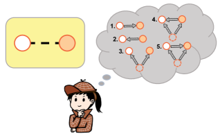
Figure 1: Quantum causal inference problem. The observer gains data from observing two quantum systems $A$ (white ball) and $B$ (red ball) which may be correlated. In line with Reichenbach’s principle, we allow for five possible causal structures: 1) $A$ has direct influence on $B$; 2) $B$ has a direct influence on $A$; 3) there is a common cause (dashed ball) acting on $A$ and $B$, meaning correlations in the initial state; 4) a combination of cases 1 and 3; 5) a combination of cases 2 and 3. The observer wants to determine which of those possible causal structures is the case.

We here address and resolve this question for the case of bipartite quantum systems of arbitrary finite dimension and measurements at two times. To be precise, we formulate the quantum causal inference problem as follows. As shown in FIG. 1, the observer has data from observing two quantum systems $A$ and $B$ which may be correlated. The observer wants to know the causal structure of the process of generating the data. In line with Reichenbach’s principle [1] we allow for five causal structures that are to be distinguished (see FIG. 1). We exclude the case of causal influence in both directions (loops), such that there is a well-defined causal direction [2]. We devise an explicit scheme for determining which causal structure is indeed the case. The scheme only employs coarse-grained projective measurements. The scheme is derived via the pseudo-density matrix (PDM) formalism, which assigns a PDM to the full data table of experiments involving measurements on systems at several times [12].

This work is organized as follows. First, we introduce the PDM formalism. Second, we present the main results, the closed-form of the $m$-time $n$-qubit PDM and our scheme for quantum causal inference. The detailed mathematical derivations are given in the Appendix. Third, we present two examples to demonstrate our scheme. Finally, we discuss the opportunities engendered by this work.

PDM formalism for measurements at multiple times, systems. The pseudo-density matrix (PDM) formalism, developed to treat space and time equally [12], provides a general framework for dealing with spatial and causal (temporal) correlations. Research on single-qubit PDMs has yielded fruitful results [34, 35, 36, 37, 38, 39, 40, 41, 42]. For example, recent studies have utilized quantum causal correlations to set limits on quantum communication [42] and to understand how dynamics emerge from temporal entanglement [37]. Furthermore, the PDM approach has been used to resolve causality paradoxes associated with closed time-like curves [39].

The PDM generalises the standard quantum $n$-qubit density matrix to the case of multiple times. The PDM is defined as

$$R_{1...m}=\frac{1}{2^{mn}}\sum^{4^{n}-1}_{i_{1}=0}...\sum^{4^{n}-1}_{i_{m}=0}\langle\{\tilde{\sigma}_{i_{\alpha}}\}^{m}_{\alpha=1}\rangle\bigotimes^{m}_{\alpha=1}\tilde{\sigma}_{i_{\alpha}},$$ (1)

where $\tilde{\sigma}_{i_{\alpha}}\in\{\sigma_{0},\sigma_{1},\sigma_{2},\sigma_{3}\}^{\otimes n}$ is an $n$-qubit Pauli matrix at time $t_{\alpha}$. $\tilde{\sigma}_{i_{\alpha}}$ is extended to an observable associated with $m$ times, $\bigotimes^{m}_{\alpha=1}\tilde{\sigma}_{i_{\alpha}}$ that has expectation value $\langle\{\tilde{\sigma}_{i_{\alpha}}\}^{m}_{\alpha=1}\rangle$. We shall return later to what measurement this expectation value corresponds to. The standard quantum density matrix is recovered if the Hilbert spaces for all but one time, say $t_{\alpha^{\prime}}$ are traced out, i.e., $\rho_{\alpha^{\prime}}=\Tr_{\alpha\neq\alpha^{\prime}}R_{1...m}$. The PDM is Hermitian with unit trace but may have negative eigenvalues.

The negative eigenvalues of the PDM appear in a measure of temporal entanglement known as a causal monotone $f(R)$ [12]. Analogously to the case of entanglement monotones [43], in general $f(R)$ is required to satisfy the following criteria: (I) $f(R)\geq 0$, (II) $f(R)$ is invariant under local change of basis, (III) $f(R)$ is non-increasing under local operations, and (IV) $\sum_{i}p_{i}f(R_{i})\geq f(\sum p_{i}R_{i})$. Those criteria are satisfied by [12]

$$f(R):=||R||_{tr}-1=\Tr\sqrt{RR^{\dagger}}-1.$$ (2)

If $R$ has negativity, $f(R)>0$. An intuition for why $f(R)$ serves as a sign of causal influence is that negative eigenvalues tell you that the PDM is associated with measurements at multiple times; in the case of a single time, there would be a standard density matrix with no negativity.

The PDM negativity $f(R)$ can thus be used to distinguish, at least in some cases, whether the PDM corresponds to two qubits at one time or one qubit at two times. This can be viewed as a simple form of causal inference, raising the question of whether the inference involving two parties (of multiple qubits) at multiple times depicted in FIG. 1 can be undertaken in a similar manner. A key challenge in this direction is to find a closed-form expression for the PDM $R$, from which one can see whether $f(R)>0$.

Closed form for m-time n-qubit PDMs. We derive a closed-form expression for the PDM for $n$ qubits and $2$ times, before generalising the expression to $m$ times.

Consider the PDM of $n$ qubits undergoing a channel $\mathcal{M}_{2|1}$ between times $t_{1}$ and $t_{2}$. In order to fully define the PDM of Eq. (1) it is necessary to further define how the Pauli expectation values $\langle\{\tilde{\sigma}_{i_{\alpha}}\}^{m}_{\alpha=1}\rangle$ are measured, since that choice impacts the states in between the measurements. We, importantly, choose coarse-grained projectors

$$\Bigl{\{} P^{\alpha}_{+}=\frac{\mathbbm{1}+\tilde{\sigma}_{i_{\alpha}}}{2},P^{\alpha}_{-}=\frac{\mathbbm{1}-\tilde{\sigma}_{i_{\alpha}}}{2}\Bigl{\}},$$ (3)

where $\alpha$ in $i_{\alpha}$ labels the time of the measurement. The coarse-grained projectors, by inspection, correspond to a minimally invasive measurement for determining the expectation values $\langle\{\tilde{\sigma}_{i_{\alpha}}\}^{m}_{\alpha=1}\rangle$.

The closed form of the PDM that we shall derive employs the Choi-Jamiołkowski (CJ) matrix of the quantum channel $\mathcal{M}_{2|1}$, defined as [44, 45]

$$M_{12}:=\sum^{2^{n}-1}_{i,j=0}\ket{i}\bra{j}^{T}\otimes\mathcal{M}_{2|1}\left(\ket{i}\bra{j}\right),$$ (4)

where the superscript $T$ denotes the transpose. We show (see the Appendix) that the 2-time $n$-qubit PDM, under coarse-grained measurements, can be written in a surprisingly neat form in terms of $M_{12}$.

Theorem 1.

Consider a system consisting of $n$ qubits with the initial state $\rho_{1}$. The coarse-grained measurements of Eq. (3) are applied at times $t_{1}$ and $t_{2}$. The channel $\mathcal{M}_{2|1}$ with CJ matrix $M_{12}$ is applied in-between the measurements. The $n$-qubit PDM can then be written as

$$R_{12}=\frac{1}{2}(M_{12}\,\rho+\rho\,M_{12}),$$ (5)

where $\rho:=\rho_{1}\otimes\mathbbm{1}_{2}$.

This extends an earlier known form for the single qubit case [34, 38].

We next stretch the argument to multiple times. Consider initially an $n$-qubit state $\rho_{1}$ measured at time $t_{1}$, undergoing the channel $\mathcal{M}_{2|1}$, measured at time $t_{2}$, undergoing $\mathcal{M}_{3|2}$ and measured at time $t_{3}$. The central objects to determine are the joint expectation values of the observables at three times. These can be written as

$$\langle\tilde{\sigma}_{i_{1}},\tilde{\sigma}_{i_{2}},\tilde{\sigma}_{i_{3}}\rangle$$

$$= \Tr_{23}[M_{23}\Bigl{(}P^{2}_{+}\rho_{2}^{(\tilde{\sigma}_{i_{1}})}P^{2}_{+}-P^{2}_{-}\rho_{2}^{(\tilde{\sigma}_{i_{1}})}P^{2}_{-}\Bigl{)}\otimes\tilde{\sigma}_{i_{3}}],$$ (6)

where we denote the CJ matrices for channels $\mathcal{M}_{2|1},\mathcal{M}_{3|2}$ by $M_{12},M_{23}$ respectively, and (see the Appendix)

$$\rho_{2}^{(\tilde{\sigma}_{i_{1}})}=\Tr_{1}[R_{12}\,\tilde{\sigma}_{i_{1}}\otimes\mathbbm{1}_{2}].$$ (7)

Eqs. (Quantum Causal Inference with Extremely Light Touch) and (7) then together imply

$$\langle\tilde{\sigma}_{i_{1}},\tilde{\sigma}_{i_{2}},\tilde{\sigma}_{i_{3}}\rangle$$

$$= \frac{1}{2}\Tr[(M_{23}R_{12}+R_{12}M_{23})\tilde{\sigma}_{i_{1}}\otimes\tilde{\sigma}_{i_{2}}\otimes\tilde{\sigma}_{i_{3}}].$$ (8)

From Eq.(Quantum Causal Inference with Extremely Light Touch), demanding that

$$R_{123}=\frac{1}{2}(R_{12}M_{23}+M_{23}R_{12}),$$ (9)

gives expectation values consistent with the PDM definition of Eq. (1). Then, since the expectation values uniquely determine the PDM, Eq. (9) must be the correct expression.

The above derivation can be directly generalized (see the Appendix) to the $m$-time $n$-qubit case.

Theorem 2.

The $n$-qubit PDM across $m$ times is given by the following iterative expression

$$R_{12...m}=\frac{1}{2}(R_{12...m-1}M_{m-1,m}+M_{m-1,m}R_{12...m-1})$$ (10)

with the initial condition $R_{12}=\frac{1}{2}(\rho\,M_{12}+M_{12}\,\rho)$ where $M_{m-1,m}$ denotes the CJ matrix of the $(m-1)$-th channel.

This iterative expression can be written in a (possibly long) closed form sum in a natural manner. We have thus extended a key tool in the PDM formalism from the cases of single qubits, two times or two qubits single time to the case of $n$ qubits at $m$ times for any $n$ and $m$.

Relating PDM negativity to causal inference. We will now consider how the negativity or positivity of reduced (partially traced) PDMs relates to the causal structure.

There are several reduced PDMs to consider. The total PDM here is associated with a bipartite system $AB$ consisting of $n$ qubits across two times $t_{1},t_{2}$, as depicted in FIG. 1. The main reduced PDMs we shall employ to infer causation are $R_{A_{1}B_{2}},R_{B_{1}A_{2}},$ where the letters denote the party and the subscripts the time. One can show (see the Appendix) $R_{A_{1}B_{2}}=\Tr_{A_{2}B_{1}}R_{A_{1}B_{1}A_{2}B_{2}},R_{B_{1}A_{2}}=\Tr_{B_{2}A_{1}}R_{A_{1}B_{1}A_{2}B_{2}}$ .

Our approach to quantum causal inference is based on analyzing the causal strength measure $f$ of Eq. (2), which measures the negativity of the PDM. The PDM is positive if there is no causal influence between the two parties [12]. However, for channels that permit causal influence, the PDM can still be positive, for properly chosen initial states (see the examples later).

We shall use certain definitions and results concerning quantum evolutions (channels) that help us distinguish whether causal influence is permitted. Those results concern so-called semicausal channels and special cases of semicausal channels. In stating these results, we will borrow some of the terminologies from Refs. [46, 47]. Semicausal channels are those bipartite completely positive trace-preserving (CPTP) maps that do not allow one party to signal or influence the other. It was proved in Ref. [47] that semicausal channels are equivalent to semilocalizable channels. A bipartite channel $\mathcal{P}$ is semilocalizable if and only if there exist channels $\mathcal{M}_{BC},\mathcal{N}_{AC}$ such that $\mathcal{P}=\Tr_{C}\mathcal{M}_{BC}\circ\mathcal{N}_{AC}$ or $\mathcal{P}=\Tr_{C}\mathcal{N}_{AC}\circ\mathcal{M}_{BC}$. The circuit representation of $\mathcal{P}=\Tr_{C}\mathcal{M}_{BC}\circ\mathcal{N}_{AC}$ is depicted in FIG. 2. A bipartite channel is called causal if it does not allow influences or signaling in either direction. A class of such channels is called localizable channels, which take the form $\mathcal{P}=\sum_{i}p_{i}\mathcal{P}_{A,i}\otimes\mathcal{P}_{B,i}.$

In our causal inference scheme to distinguish between the causal structures of FIG. 1 one of the causal structures allowed is semicausal channels between $A$ and $B$ [47]. For example, as shown in FIG. 2, there may be a physical process $\mathcal{P}$ on $A$ and $B$ across two times $t_{1},t_{2}$ that can be decomposed into $\mathcal{M}_{BC}\circ\mathcal{\mathcal{N}}_{AC}$ where $A$ can influence $B$ and the inverse is not true.

The following theorem plays a crucial role in the causal inference scheme we shall propose. The theorem concerns the case of semi-causal channels, i.e. of signalling in one direction only. It shows that, for semi-causal channels, a particular PDM will have no negativity regardless of the bipartite input state to the process.

Theorem 3 (null PDM negativity for semicausal channels).

If a quantum channel $\mathcal{P}$ does not allow signaling from $B$ to $A$, i.e., semicausal, then, for any state $\rho_{A_{1}B_{1}}$ at time $t_{1}$, the PDM $R_{B_{1}A_{2}}$ is positive semidefinite and the PDM negativity $f(R_{B_{1}A_{2}})=0$.

This theorem is quite remarkable. It shows that if there is no causation from $B_{1}$ to $A_{2}$, any initial correlations between $A_{1}$ and $B_{1}$ cannot make the PDM negativity $f(R_{B_{1}A_{2}})>0$. In contrast, other measures ‘without intervention’ are impacted by initial correlations [48]. Moreover, the theorem implies that only the existence of causal influence between $B$ and $A$ allows for $f(R_{B_{1}A_{2}})>0$. Finally, constructing $R_{B_{1}A_{2}}$ and $R_{B_{2}A_{1}}$ only requires restricted statistics, and not full knowledge of the channel.

The following Corollary follows immediately from Theorem 3.

Corollary 1.

If a quantum channel $\mathcal{P}$ does not allow signaling in both directions, i.e., is causal, then, for any state $\rho_{A_{1}B_{1}}$ at time $t_{1}$, the two PDMs $R_{B_{1}A_{2}}$, $R_{A_{1}B_{2}}$ are positive semidefinite and the PDM negativities $f(R_{B_{1}A_{2}})=f(R_{A_{1}B_{2}})=0$.

If one is free to choose input states as part of characterising solely the channel, like in Refs. [46, 47], using pure input states can be seen to be optimal. From property IV of $f(.)$, with a given $R=\sum_{i}p_{i}R_{i}$, the most negative pure state $R_{i*}:=\mathrm{argmax}\,f(R_{i})$ respects $f(R_{i*})\geq f(R)$. We conjecture that there is always a family of pure input states such that the sign of $f$ determines whether a channel is signalling in a given direction–see the Appendix for a proof of this for the case of 2-qubit unitary evolution.

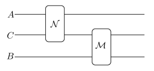
Figure 2: Semicausal channel. Semicausal channels are equivalent to semilocalizable channels [47]. A channel acting on two parties $A$ and $B$ is called semilocalized if it can be decomposed into either $\mathcal{M}_{BC}\circ\mathcal{\mathcal{N}}_{AC}$ or $\mathcal{N}_{AC}\circ\mathcal{\mathcal{M}}_{BC}$ where $C$ is an ancilla, as in the above circuit. One sees that in this example $A$ can causally influence $B$ while the inverse is not true.

Protocol for Quantum causal inference via measurements alone. Our approach to quantum causal inference from the PDM $R_{A_{1}B_{1}A_{2}B_{2}}$ involves two tasks, with the protocol for the second task making direct use of Theorem 3.

• Identify whether there is a common cause of $\rho_{A_{2}B_{2}}=R_{A_{2}B_{2}}$ (the possible presence of which is depicted via dashed ball in FIG.1). This means determining whether there are correlations in $\rho_{A_{1}B_{1}}=R_{A_{1}B_{1}}$, as can be done by standard methods once $\rho_{A_{1}B_{1}}$ is known. $\rho_{A_{1}B_{1}}$, in turn, can be deduced from the total PDM $R$ via $\rho_{A_{1}B_{1}}=\Tr_{2}R_{A_{1}B_{1}A_{2}B_{2}}$.

• Identify the cause-effect direction (the direction of the arrow between the white and red ball in FIG. 1). Once we have constructed the PDMs $R_{A_{1}B_{2}},R_{B_{1}A_{2}}$, we calculate the PDM negativities $f(R_{A_{1}B_{2}}),f(R_{B_{1}A_{2}}).$ Given Theorem 3 we can infer the cause-effect relation from these causal strengths. More specifically, there are three cases:

  • $f(R_{A_{1}B_{2}})>0,f(R_{B_{1}A_{2}})=0$. Then the causal direction is $A\rightarrow B$;

  • $f(R_{A_{1}B_{2}})=0,f(R_{B_{1}A_{2}})>0$. Then the causal direction is $A\leftarrow B$;

  • $f(R_{A_{1}B_{2}})=0,f(R_{B_{1}A_{2}})=0$. Then we are not sure about the causal direction. Either there is no causal influence between the two parties, as demonstrated by the corollary to Theorem 3, or the channel permits causal influence, but the initial states are chosen in such a way that the PDMs $R_{A_{1}B_{2}},R_{B_{1}A_{2}}$ are positive.

Example: consecutive swaps with initial correlation. We firstly illustrate the causal inference protocol with an example that is straightforward to calculate analytically. Suppose that the initial state $\rho_{1}=\ket{\Psi}_{ABC}\bra{\Psi}$ where $\ket{\Psi}_{ABC}=\frac{1}{\sqrt{2}}(\ket{000}+\ket{111})$. This state, as shown in FIG. 2, undergoes swap channels $\mathcal{N}_{AC}=\text{swap}(A,C)$ and $\mathcal{M}_{BC}=\text{swap}(B,C)$. In the Pauli basis , the CJ matrix of the channel $\mathcal{M}_{BC}\circ\mathcal{N}_{AC}$ (Eq. (4)) can be written as

$$M=\frac{1}{2^{3}}\sum^{3}_{ijk=0}\sigma_{i}\sigma_{j}\sigma_{k}\ \mathcal{M}_{BC}\circ\mathcal{N}_{AC}(\sigma_{i}\sigma_{j}\sigma_{k}),$$ (11)

where the tensor products ‘$\otimes$’ are implicit.

We assume the experimenter has undertaken measurements determining the PDM $R_{A_{1}B_{1}C_{1}A_{2}B_{2}C_{2}}$. Given Eq. (5), the PDM for the three systems is in fact

$$R_{A_{1}B_{1}C_{1}A_{2}B_{2}C_{2}}=\frac{1}{2}(M\rho+\rho M).$$ (12)

Recall that $R_{A_{1}B_{2}}=\Tr_{B_{1}C_{1}A_{2}C_{2}}R_{A_{1}B_{1}C_{1}A_{2}B_{2}C_{2}}$ and $R_{B_{1}A_{2}}=\Tr_{A_{1}C_{1}B_{2}C_{2}}R_{A_{1}B_{1}C_{1}A_{2}B_{2}C_{2}}$. We obtain $R_{A_{1}B_{2}}=\frac{1}{4}\sum^{3}_{i=0}\sigma_{i}\otimes\sigma_{i}\,$ with eigenvalues $\{-\frac{1}{2},\frac{1}{2},\frac{1}{2},\frac{1}{2}\}$. Moreover, $R_{B_{1}A_{2}}=\frac{1}{4}\left(\sigma_{0}\otimes\sigma_{0}+\sigma_{3}\otimes\sigma_{3}\right)\,$ with eigenvalues $\{\frac{1}{2},\frac{1}{2},0,0\}$. The PDM negativities $f(R_{A_{1}B_{2}})=1>0,f(R_{B_{1}A_{2}})=0.$ Therefore, $A$ has causal influence on $B$. Moreover, we saw that the initial state has correlation. Thus we have, from the total $R$, inferred that the causal structure is of type 5 in FIG. 1.

The example also illustrates how the protocol allows one to infer the causal relationship solely from correlations of coarse-grained quantum measurements. The protocol only requires $R$ which is determined via correlations of quantum measurements that we chose to be coarse-grained. This contrasts with the reset interventions which are commonly employed in classical causal inference problems [2]. Quantum measurements do in general disturb the system, but much less so than resets, and moreover, our protocol only requires coarse-grained measurements.

Example: measure-and-prepare channel with or without initial correlation. We now consider an example, related to Ref. [25], that shows how our light-touch protocol can resolve the causal structure even for channels that do not preserve quantum coherence. Let systems $A$ and $B$ be single qubit systems and the end effect of the compound channel $\mathcal{M}_{BC}\circ\mathcal{N}_{AC}$ on the compound system $AB$ be the channel that measures the system $A$ and then prepares a state on system $B$. Denote the effective channel on $AB$ by $\mathcal{L}_{A\rightarrow B}$. We demand that the action of $\mathcal{L}_{A\rightarrow B}$ on the state is $\mathcal{L}_{A\rightarrow B}(\rho_{A})=\bra{0}\rho_{A}\ket{0}\ket{0}_{B}\bra{0}+\bra{1}\rho_{A}\ket{1}\ket{1}_{B}\bra{1}$. Therefore, the CJ matrix of $\mathcal{L}$ in the Pauli basis is

$$M_{A_{1}B_{2}}=\frac{1}{2}\sum^{3}_{i=0}\sigma_{i}\otimes\mathcal{L}(\sigma_{i})=\frac{1}{2}(\sigma_{0}\otimes\sigma_{0}+\sigma_{3}\otimes\sigma_{3}).$$ (13)

Substituting Eq. (13) into Eq. (5), the PDM

$$R_{A_{1}B_{2}}= \left(\frac{1}{2}\rho_{A_{1}}+\frac{1}{4}\sigma_{3}+\frac{z}{4}\sigma_{0}\right)\otimes\ket{0}\bra{0}$$

$$+\left(\frac{1}{2}\rho_{A_{1}}-\frac{1}{4}\sigma_{3}-\frac{z}{4}\sigma_{0}\right)\otimes\ket{1}\bra{1},$$ (14)

where $z:=\Tr(\rho_{A_{1}}\sigma_{3})$. The eigenvalues of $\rho_{A_{1}}+\frac{1}{2}\sigma_{3}+\frac{z}{2}\mathbbm{1}$ are $\frac{1}{2}(1+z\pm\sqrt{(1+z)^{2}+x^{2}+y^{2}})$ with $x:=\Tr(\rho_{A_{1}}\sigma_{1}),y:=\Tr(\rho_{A_{1}}\sigma_{2})$. Thus, the PDM is negative exactly when $x^{2}+y^{2}>0$, i.e., when the initial state $\rho_{A_{1}}$ is coherent in the Pauli-$z$ basis. Then, for example, when the PDM $R_{A_{1}B_{2}}$ is negative, the causal direction is from $A$ to $B$ (case 1 or 5 in FIG. 1). The initial state would determine the exact causal relation.

The above example highlights how our scheme can resolve the causal structure solely from observational data in a decoherent channel. This goes beyond the observational scheme in Ref. [25] and shows that coherence in the channel is not required here for the apparent quantum advantage in resolving causal relations, but rather coherence in the initial state.

Summary and outlook. We showed that quantum observations alone are sufficient to resolve causal relations for the case of bipartite quantum systems with measurements at two times. We showed this by, firstly, deriving as a key technical contribution a closed-form expression for the space-time pseudo-density matrix associated with many times and qubits. We show that this matrix can be determined by coarse-grained quantum observations alone and that given the matrix one can infer the causal structure via the sign of a causal monotone function. The scheme thus amounts to an extremely light-touch quantum causal inference protocol. The protocol shows how in the quantum case, for any bipartite system, one can in fact, in opposition to the slogan ‘correlation does not imply causation’ infer causal relationships from correlations between measurement outcomes, provided these are at several times. We showed that here, the quantum advantage in inferring causal structures lies in the coherence present in the initial state.

The results naturally point towards several developments:(i) While the derivation of Leggett-Garg type inequalities typically assumes no evolution between measurements [9, 49], our closed-form expression enables deriving inequalities for arbitrary evolutions, (ii) The causality monotone might be possible to witness via observables, taking inspiration from [50], (iii) These results could perhaps have been derived in other formalisms based around the CJ isomorphism [51, 10, 18, 16, 19, 25], (iv) Our scheme can be used to determine classical causal structures without interventions provided that these can be probed in quantum superposition, e.g. as in the case of typical optical table equipment, (v) What does it tell us about quantum theory that such light-touch interventions are sufficient to determine the causal structure, apparently in sharp contrast to the classical case?

Acknowledgements. We thank Dong Yang, Daniel Ebler, Caslav Brukner, Giulio Chiribella and James Fullwood for discussions. XL and OD acknowledge support from the NSFC (Grants No. 12050410246, No. 1200509, No. 12050410245) and City University of Hong Kong (Project No. 9610623). YQ is supported by the NRF, Singapore and A*STAR. This publication was made possible in part through the support of the ID 61466 grant from the John Templeton Foundation, as part of the The Quantum Information Structure of Spacetime (QISS) Project (qiss.fr). The opinions expressed in this publication are those of the authors and do not necessarily reflect the views of the John Templeton Foundation. This research is also funded in part by the Gordon and Betty Moore Foundation through Grant GBMF10604 to VV.

Measurement scheme. Let us take a two-qubit system to illustrate our design of measurement events. At initial time $t_{1}$, we implement the observable $\sigma_{i}^{A}\otimes\sigma_{j}^{B}$. This observable can be decomposed into linear combinations of projectors in several ways. For example,

$$\sigma_{i}\otimes\sigma_{j} =P_{1}+P_{2}-P_{3}-P_{4}=(P_{1}+P_{2})-(P_{3}+P_{4}),$$ (15)

where

$$P_{1}:=\frac{1}{4}(\mathbbm{1}+\sigma_{i})\otimes(\mathbbm{1}+\sigma_{j}),\,P_{2}:=\frac{1}{4}(\mathbbm{1}-\sigma_{i})\otimes(\mathbbm{1}-\sigma_{j}),\,$$

$$P_{3}:=\frac{1}{4}(\mathbbm{1}+\sigma_{i})\otimes(\mathbbm{1}-\sigma_{j}),\,P_{4}:=\frac{1}{4}(\mathbbm{1}-\sigma_{i}),\otimes(\mathbbm{1}+\sigma_{j}),$$ (16)

are the elements of the projective measurement. It can also be decomposed in terms of the Bell basis

$$\sigma_{i}\otimes\sigma_{j} =\tilde{P}_{1}+\tilde{P}_{2}-\tilde{P}_{3}-\tilde{P}_{4}=(\tilde{P}_{1}+\tilde{P}_{2})-(\tilde{P}_{3}+\tilde{P}_{4}),$$ (17)

where

$$\tilde{P}_{1} :=\frac{1}{4}U(\mathbbm{1}\otimes\mathbbm{1}+\sigma_{1}\otimes\sigma_{1}-\sigma_{2}\otimes\sigma_{2}+\sigma_{3}\otimes\sigma_{3})U^{\dagger},\tilde{P}_{2}:=\frac{1}{4}U(\mathbbm{1}\otimes\mathbbm{1}+\sigma_{1}\otimes\sigma_{1}+\sigma_{2}\otimes\sigma_{2}-\sigma_{3}\otimes\sigma_{3})U^{\dagger},$$

$$\tilde{P}_{3} :=\frac{1}{4}U(\mathbbm{1}\otimes\mathbbm{1}-\sigma_{1}\otimes\sigma_{1}+\sigma_{2}\otimes\sigma_{2}+\sigma_{3}\otimes\sigma_{3})U^{\dagger},\tilde{P}_{4}:=\frac{1}{4}U(\mathbbm{1}\otimes\mathbbm{1}-\sigma_{1}\otimes\sigma_{1}-\sigma_{2}\otimes\sigma_{2}-\sigma_{3}\otimes\sigma_{3})U^{\dagger},$$ (18)

are elements of the Bell measurement with the unitary $U$ satisfying $U\sigma_{1}\otimes\sigma_{1}U^{\dagger}=\sigma_{i}\otimes\sigma_{j}.$

One can show

$$P_{1}+P_{2}=\tilde{P}_{1}+\tilde{P}_{2}=:P_{+},$$ (19)

and

$$P_{3}+P_{4}=\tilde{P}_{3}+\tilde{P}_{4}=:P_{-}.$$ (20)

We shall define the PDM in terms of the corresponding coarse-grained measurement

$$\Bigl{\{}P_{+}:=\frac{\mathbbm{1}\otimes\mathbbm{1}+\sigma_{i}\otimes\sigma_{j}}{2},P_{-}:=\frac{\mathbbm{1}\otimes\mathbbm{1}-\sigma_{i}\otimes\sigma_{j}}{2}\Bigl{\}}.$$

The 2-time $n$-qubit PDM. Having the quantum state $\rho_{1}$ at time $t_{1}$, the measurement $\{P^{\alpha}_{+},P^{\alpha}_{-}\}$ at each time $t_{\alpha},\alpha=1,2,$ and the quantum channel $\mathcal{M}_{2|1}$ with its CJ matrix $M_{12}$, we are in a good position to obtain the 2-time $n$-qubit PDM. Recall that the general form of $n$-qubit PDM across two times $[t_{1},t_{2}]$ is given by

$$R_{12}=\frac{1}{2^{2n}}\sum^{4^{n}-1}_{i_{1}=0}\sum^{4^{n}-1}_{i_{2}=0}\langle\tilde{\sigma}_{i_{1}},\tilde{\sigma}_{i_{2}}\rangle\,\tilde{\sigma}_{i_{1}}\otimes\tilde{\sigma}_{i_{2}}.$$ (21)

Therefore, in order to construct the PDM, it is necessary to calculate the expectation values of the product of the result of the measurements, i.e., $\langle\tilde{\sigma}_{i_{1}},\tilde{\sigma}_{i_{2}}\rangle$. According to the definition of the PDM, the initial state collapse to the eigenstates of the $n$-qubit Pauli matrix $\tilde{\sigma}_{i_{1}}$ after the measurement at time $t_{1}$. Then the post-measurement states go through the channel followed by a measurement at time $t_{2}$. Denote $\{P^{\alpha}_{+}=(\mathbbm{1}+\tilde{\sigma}_{i_{\alpha}})/2,P^{\alpha}_{-}=(\mathbbm{1}-\tilde{\sigma}_{i_{\alpha}})/2\}$ by the coarse-grained measurement scheme at time $t_{\alpha},\alpha=1,2$, the product of expectation values can be expressed by

$$\langle\tilde{\sigma}_{i_{1}},\tilde{\sigma}_{i_{2}}\rangle=\Tr[M_{12}(P^{1}_{+}\rho_{1}P^{1}_{+}\otimes\tilde{\sigma}_{i_{2}})]-\Tr[M_{12}(P^{1}_{-}\rho_{1}P^{1}_{-}\otimes\tilde{\sigma}_{i_{2}})],$$ (22)

It is straightforward to calculate that

$$P^{1}_{+}\rho_{1}P^{1}_{+}-P^{1}_{-}\rho_{1}P^{1}_{-}=\frac{\mathbbm{1}+\tilde{\sigma}_{i_{1}}}{2}\rho_{1}\frac{\mathbbm{1}+\tilde{\sigma}_{i_{1}}}{2}-\frac{\mathbbm{1}-\tilde{\sigma}_{i_{1}}}{2}\rho_{1}\frac{\mathbbm{1}-\tilde{\sigma}_{i_{1}}}{2}=\frac{1}{2}(\rho_{1}\tilde{\sigma}_{i_{1}}+\tilde{\sigma}_{i_{1}}\rho_{1}).$$ (23)

Substituting Eq (23) into Eq (22) leads to

$$\langle\tilde{\sigma}_{i_{1}},\tilde{\sigma}_{i_{2}}\rangle= \Tr[\frac{1}{2}M_{12}(\rho_{1}\tilde{\sigma}_{i_{1}}+\tilde{\sigma}_{i_{1}}\rho_{1})\otimes\tilde{\sigma}_{i_{2}}]$$

$$= \Tr[\frac{1}{2}(M_{12}\,\rho_{1}\otimes\mathbbm{1}_{2}+\rho_{1}\otimes\mathbbm{1}_{2}\,M_{12})\tilde{\sigma}_{i_{1}}\otimes\tilde{\sigma}_{i_{2}}]$$

$$\equiv \Tr[R_{12}\tilde{\sigma}_{i_{1}}\otimes\tilde{\sigma}_{i_{2}}].$$ (24)

where the cyclic property of the trace is used in the second equality. Finally, the two-qubit PDM is expressed by

$$R_{12}=\frac{1}{2}(M\rho+\rho M).$$ (25)

where $\rho:=\rho_{1}\otimes\mathbbm{1}_{2}$.

In the following, we verify that the PDM given by Eq. (25) returns to the normal density matrix when there is one time point left.

• Tracing out the final time $t_{2}$, the PDM returns to the initial state,

  $$\Tr_{2}R_{12}=\frac{1}{2}\Tr_{2}(M_{12}\,\rho+\rho\,M_{12})=\rho_{1},$$ (26)

  where $\Tr_{2}M_{12}=\mathbbm{1}_{1}$ is used in the second equality,

• Tracing out the initial time $t_{1}$, the PDM returns to the output state,

  $$\Tr_{1}R_{12}=\frac{1}{2}\Tr_{1}(M_{12}\,\rho+\rho\,M_{12})=\Tr_{1}M_{12}\,\rho_{1}\otimes\mathbbm{1}_{2}=\mathcal{M}_{2|1}(\rho_{1}),$$ (27)

  where the cyclic property of the trace is used in the second equality.

The $m$-time $n$-qubit PDM. In this section, we extend the $n$-qubit PDM formalism to across $m$ times. To do that we first consider an $n$-qubit state $\rho$ at time $t_{1}$ that undergoes the channel $\mathcal{M}_{2|1}$, arrives at time $t_{2}$, then experiences channel $\mathcal{M}_{3|2}$ and arrives at time $t_{3}$. Denote the CJ matrices for channels $\mathcal{M}_{2|1},\mathcal{M}_{3|2}$ by $M_{12},M_{23}$ respectively. The tensor product ‘$\otimes$’ is sometimes omitted when there is no confusion.

We first recall that the two-time $n$-qubit PDM takes the form

$$R_{12}=\frac{1}{2}(M_{12}\rho+\rho M_{12}).$$ (28)

We now proceed to derive a closed form of the 3-time $n$-qubit PDM. To do that, it is sufficient to calculate the expectation values of measurement events. Consider measurement events at time $t_{1},t_{2},t_{3}$ are $\{\tilde{\sigma}_{i_{1}}\},\{\tilde{\sigma}_{i_{2}}\},\{\tilde{\sigma}_{i_{3}}\}$, respectively. The initial state $\rho_{1}$ first collapses to the eigenstates of operator $\tilde{\sigma}_{i_{1}}$ then goes into the channel $\mathcal{M}_{2|1}$. The central quantity we wish to evaluate is $\langle\tilde{\sigma}_{i_{1}},\tilde{\sigma}_{i_{2}},\tilde{\sigma}_{i_{3}}\rangle$.

Our expression for $\langle\tilde{\sigma}_{i_{1}},\tilde{\sigma}_{i_{2}},\tilde{\sigma}_{i_{3}}\rangle$ will turn out to involve a matrix $\rho_{2}^{(\tilde{\sigma}_{i_{1}})}$. We now derive a simplified expression for $\rho_{2}^{(\tilde{\sigma}_{i_{1}})}$, which we shall use later.

$$\rho_{2}^{(\tilde{\sigma}_{i_{1}})}:= \Tr_{1}[\frac{1}{2}(M_{12}P^{1}_{+}\rho_{1}P^{1}_{+}+P^{1}_{+}\rho_{1}P^{1}_{+}M_{12})]-\Tr_{1}[\frac{1}{2}(M_{12}P^{1}_{-}\rho_{1}P^{1}_{-}+P^{1}_{-}\rho_{1}P^{1}_{-}M_{12})]$$

$$= \Tr_{1}[\frac{1}{2}M_{12}(P^{1}_{+}\rho_{1}P^{1}_{+}-P^{1}_{-}\rho_{1}P^{1}_{-})]+\Tr_{1}[\frac{1}{2}(P^{1}_{+}\rho_{1}P^{1}_{+}-P^{1}_{-}\rho_{1}P^{1}_{-})M_{12}]$$

$$= \Tr_{1}[\frac{1}{4}M_{12}(\rho_{1}\tilde{\sigma}_{i_{1}}+\tilde{\sigma}_{i_{1}}\rho_{1})]+\Tr_{1}[\frac{1}{4}(\rho_{1}\tilde{\sigma}_{i_{1}}+\tilde{\sigma}_{i_{1}}\rho_{1})M_{12}]$$

$$= \Tr_{1}[\frac{1}{2}(M_{12}\rho_{1}+\rho_{1}M_{12})\tilde{\sigma}_{i_{1}}]$$

$$= \Tr_{1}[R_{12}\tilde{\sigma}_{i_{1}}],$$ (29)

where the identity operators $\mathbbm{1}_{2}$ at time $t_{2}$ are ignored throughout the calculation, Eq. (23) is used in the third equality and the cyclic property of the trace is used in the fourth equality. Then, the expectation value of the product of measurement outcomes at three time points is given by

$$\langle\tilde{\sigma}_{i_{1}},\tilde{\sigma}_{i_{2}},\tilde{\sigma}_{i_{3}}\rangle$$

$$= \Tr_{23}[M_{23}\Bigl{(}P^{2}_{+}\rho^{(\tilde{\sigma}_{i_{1}})}_{2}P^{2}_{+}-P^{2}_{-}\rho^{(\tilde{\sigma}_{i_{1}})}_{2}P^{2}_{-}\Bigl{)}\otimes\tilde{\sigma}_{i_{3}}]$$

$$= \frac{1}{2}\Tr_{23}[M_{23}\Bigl{(}(\Tr_{1}R_{12}\tilde{\sigma}_{i_{1}})\sigma_{i_{2}}+\tilde{\sigma}_{i_{2}}(\Tr_{1}R_{12}\tilde{\sigma}_{i_{1}})\Bigl{)}\otimes\tilde{\sigma}_{i_{3}}]$$

$$= \frac{1}{2}\Tr_{123}[M_{23}(R_{12}\tilde{\sigma}_{i_{1}})\tilde{\sigma}_{i_{2}}+(R_{12}\tilde{\sigma}_{i_{1}}M_{23})\tilde{\sigma}_{i_{2}}\Bigl{)}\otimes\tilde{\sigma}_{i_{3}}]$$

$$= \frac{1}{2}\Tr[(M_{23}R_{12}+R_{12}M_{23})\tilde{\sigma}_{i_{1}}\otimes\tilde{\sigma}_{i_{2}}\otimes\tilde{\sigma}_{i_{3}}],$$ (30)

where Eq. (23) and Eq. (Quantum Causal Inference with Extremely Light Touch) are used in the second equality and the cyclic property of the trace is used in the third equality. Thus, we have the $n$-qubit PDM across 3 times as

$$R_{123}=\frac{1}{2}(R_{12}M_{23}+M_{23}R_{12}).$$ (31)

Let us assume that we have the $(m-1)$-time $n$-qubit PDM $R_{12,...,m-1}$. We then consider $m$ events $\{\tilde{\sigma}_{i_{1}},\tilde{\sigma}_{i_{2}},...,\tilde{\sigma}_{i_{m}}\}$ and the channel $\mathcal{M}_{i+1|i}$ between time interval $[t_{i},t_{i+1}],i\in\{1,2,3,...,m-1\}$ with the corresponding CJ matrix $M_{i,i+1}$. Similarly, the matrix $\rho^{(\vec{\tilde{\sigma}})}_{m-1}$ just before measurement made at time $t_{m-1}$ can be written as

$$\rho^{(\vec{\tilde{\sigma}})}_{m-1}=\Tr_{12..,m-2}[R_{12,...,m-1}\tilde{\sigma}_{i_{1}}\tilde{\sigma}_{i_{2}}...\tilde{\sigma}_{i_{m-2}}].$$ (32)

The expectation value of the product of measurement outcomes at those time points is given by

$$\langle\tilde{\sigma}_{i_{1}},\tilde{\sigma}_{i_{2}},...,\tilde{\sigma}_{i_{m}}\rangle$$

$$= \Tr_{m-1,m}\Bigl{(}M_{m-1,m}\Bigl{(}P^{m-1}_{+}\rho^{(\vec{\tilde{\sigma}})}_{m-1}P^{m-1}_{+}-P^{m-1}_{-}\rho^{(\vec{\tilde{\sigma}})}_{m-1}P^{m-1}_{-}\Bigl{)}\tilde{\sigma}_{i_{m}}\Bigl{)}$$

$$= \frac{1}{2}\Tr_{m-1,m}\Bigl{(}M_{m-1,m}\Bigl{(}(\Tr_{12,...,m-2}R_{12,...,m-1}\tilde{\sigma}_{i_{1}}\tilde{\sigma}_{i_{2}},...,\tilde{\sigma}_{i_{m-2}})\tilde{\sigma}_{i_{m-1}}+\tilde{\sigma}_{i_{m-1}}(\Tr_{12,...,m-2}R_{12,...,m-1}\tilde{\sigma}_{i_{1}}\tilde{\sigma}_{i_{2}},...,\tilde{\sigma}_{i_{m-2}})\Bigl{)}\tilde{\sigma}_{i_{m}}\Bigl{)}$$

$$= \frac{1}{2}\Tr_{12,...,m}\Bigl{(}M_{m-1,m}(R_{12,...,m-1}\tilde{\sigma}_{i_{1}}\tilde{\sigma}_{i_{2}},...,\tilde{\sigma}_{i_{m-2}})\tilde{\sigma}_{i_{m-1}}+(R_{12,...,m-1}\tilde{\sigma}_{i_{1}}\tilde{\sigma}_{i_{2}},...,\tilde{\sigma}_{i_{m-2}})M_{m-1,m}\tilde{\sigma}_{i_{m-1}}\Bigl{)}\tilde{\sigma}_{i_{m}}\Bigl{)}$$

$$= \frac{1}{2}\Tr_{12,...,m}\Bigl{(}(M_{m-1,m}R_{12,...,m-1}+R_{12,...,m-1}M_{m-1,m})\tilde{\sigma}_{i_{1}}\tilde{\sigma}_{i_{2}}...\tilde{\sigma}_{i_{m}}\Bigl{)},$$ (33)

Thus, we have $R_{12...m}=\frac{1}{2}(R_{12...m-1}M_{m-1,m}+M_{m-1,m}R_{12...m-1})$.

In summary, the $n$-qubit PDM across $m$ times is given by the following iterative expression

$$R_{12...m}=\frac{1}{2}(R_{12...m-1}M_{m-1,m}+M_{m-1,m}R_{12...m-1})$$ (34)

with the initial condition $R_{12}=\frac{1}{2}(\rho M_{12}+M_{12}\rho)$, $M_{m-1,m}$ denotes the CJ matrix of the $(m-1)$th channel.

Partial trace. Given a pseudo-density matrix $R_{A_{1}B_{1}A_{2}B_{2}}$ defined over two sets of events $A_{1}B_{1}$ and $A_{2}B_{2}$ and a pseudo-density matrix $R_{A_{1}B_{2}}$ contructed from the sets of events $A_{1}$ and $B_{2}$, one can show that the latter can be obtained from $R_{A_{1}B_{1}A_{2}B_{2}}$ by tracing over the subsystem corresponding to $B_{1}A_{2}$, i.e., $R_{A_{1}B_{2}}=\Tr_{A_{2}B_{1}}R_{A_{1}B_{1}A_{2}B_{2}}$.

Proof.

For the simplicity of the notations, we give a proof to the two-time two-qubit PDM case, it can be directly generalized to the $m$-time $n$-qubit PDM case. In the following calculation, the tensor product ‘$\otimes$’ is omitted when there is no confusion.

From the definition of pseudo-density matrix, we have

$$R_{A_{1}B_{2}}=\frac{1}{4}\sum^{3}_{i=0}\sum^{3}_{j=0}\langle\sigma^{A_{1}}_{i},\sigma^{B_{2}}_{j}\rangle\sigma^{A_{1}}_{i}\sigma^{B_{2}}_{j},$$ (35)

and

$$R_{A_{1}B_{1}A_{2}B_{2}}=\frac{1}{2^{4}}\sum^{3}_{i,j,k,l=0}\langle\sigma^{A_{1}}_{i}\sigma^{B_{1}}_{j},\sigma^{A_{2}}_{k}\sigma^{B_{2}}_{l}\rangle\sigma^{A_{1}}_{i}\sigma^{B_{1}}_{j}\sigma^{A_{2}}_{k}\sigma^{B_{2}}_{l}.$$ (36)

It is then straightforward to calculate

$$\Tr_{B_{1}A_{2}}R_{A_{1}B_{1}A_{2}B_{2}}$$

$$= \Tr_{B_{1}A_{2}}[\frac{1}{2^{4}}\sum^{3}_{i,j,k,l=0}\langle\sigma^{A_{1}}_{i}\sigma^{B_{1}}_{j},\sigma^{A_{2}}_{k}\sigma^{B_{2}}_{l}\rangle\sigma^{A_{1}}_{i}\sigma^{B_{1}}_{j}\sigma^{A_{2}}_{k}\sigma^{B_{2}}_{l}]$$

$$= \frac{1}{2^{4}}\sum^{3}_{i,j,k,l=0}\Tr_{B_{1}A_{2}}(\sigma^{B_{1}}_{j}\sigma^{A_{2}}_{k})\langle\sigma^{A_{1}}_{i}\sigma^{B_{1}}_{j},\sigma^{A_{2}}_{k}\sigma^{B_{2}}_{l}\rangle\sigma^{A_{1}}_{i}\sigma^{B_{2}}_{l}$$

$$= \frac{1}{2^{2}}\sum^{3}_{i,j=0}\langle\sigma^{A_{1}}_{i}\sigma^{B_{1}}_{0},\sigma^{A_{2}}_{0}\sigma^{B_{2}}_{j}\rangle\sigma^{A_{1}}_{i}\sigma^{B_{2}}_{l}$$

$$= R_{A_{1}B_{2}}.$$ (37)

This completes the proof. ∎

Proof of Therem 3.

Theorem 3. If a quantum channel $\mathcal{P}$ does not allow signaling from $B$ to $A$, i.e., semicausal, then, for any state $\rho_{A_{1}B_{1}}$ at time $t_{1}$, the PDM $R_{B_{1}A_{2}}$ is positive semidefinite and the PDM negativity $f(R_{B_{1}A_{2}})=0$.

Proof.

A channel $\mathcal{P}:\mathcal{B}(\mathcal{H}_{A_{1}B_{1}})\rightarrow\mathcal{B}(\mathcal{H}_{A_{2}B_{2}})$ is called semicausal [47], if,

$$\Tr_{B_{2}}\mathcal{P}(\rho_{A_{1}B_{1}})=\mathcal{T}(\rho_{A_{1}}),$$ (38)

for all input states $\rho_{A_{1}B_{1}}$ and for some completely positive maps $\mathcal{T}:\mathcal{B}(\mathcal{H}_{A_{1}})\rightarrow\mathcal{B}(\mathcal{H}_{A_{2}})$.

For the simplicity of the notations, we give a proof to the two-qubit PDM case, it can be directly generalized to the $n$-qubit PDM case. In the Pauli basis, the CJ matrix of channel $\mathcal{P}$ is

$$M= \sum^{2^{2}-1}_{i,j=0}\ket{i}\bra{j}^{T}\otimes\mathcal{P}\left(\ket{i}\bra{j}\right)=\frac{1}{2^{2}}\sum^{3}_{i,j=0}\sigma^{A_{1}}_{i}\sigma^{B_{1}}_{j}\mathcal{P}(\sigma^{A_{1}}_{i}\sigma^{B_{1}}_{j}).$$ (39)

where the tensor products ‘$\otimes$’ are omitted. The PDM can be calculated as

$$R_{B_{1}A_{2}}= \Tr_{A_{1}B_{2}}R_{A_{1}B_{1}A_{2}B_{2}}$$

$$= \frac{1}{2}\Tr_{A_{1}B_{2}}[M\rho_{A_{1}B_{1}}+\rho_{A_{1}B_{1}}M]$$

$$= \frac{1}{8}\Tr_{A_{1}B_{2}}\sum^{3}_{i,j=0}\{\rho_{A_{1}B_{1}},\sigma^{A_{1}}_{i}\sigma^{B_{1}}_{j}\}\mathcal{P}(\sigma^{A_{1}}_{i}\sigma^{B_{1}}_{j})$$

$$= \frac{1}{8}\Tr_{A_{1}}\sum^{3}_{i=0}\{\rho_{A_{1}B_{1}},\sigma^{A_{1}}_{i}\sigma^{B_{1}}_{0}\}\mathcal{T}_{A}(\sigma^{A_{1}}_{i})$$

$$= \frac{1}{4}\sum^{3}_{i,l=0}\langle\sigma^{A_{1}}_{i}\sigma^{B_{1}}_{l}\rangle\sigma^{B_{1}}_{l}\mathcal{T}_{A}(\sigma^{A_{1}}_{i})$$

$$= \mathcal{T}_{A}\otimes\mathbbm{1}_{B}(\rho_{A_{1}B_{1}}),$$ (40)

where $\{\,,\}$ denotes the anticommutator, Eq. (39) is used in the third equality and Eq. (38) is used in the fourth equality. Since $\mathcal{T}$ is completely positive, it is straightforward to see that $R_{B_{1}A_{2}}$ is positive semidefinite. Finally, $f(R_{B_{1}A_{2}})=0$ since the causal monotone $f$ measures the negativity of PDMs. This completes the proof. ∎

Determining causal influence of channel by optimizing the input state. We conjecture that, for the case where the input state is free because one is solely interested in whether the channel is signaling, there is always a family of states such that $f>0$ provides a necessary and sufficient condition for the channel to allow causal influence in a given direction. We here show the conjecture to hold for any two-qubit unitary channel.

Any two-qubit unitary $U_{AB}$ has the following decomposition [52]

$$U_{AB}=U_{A}\otimes U_{B}\,e^{i\theta S_{AB}}\,V_{A}\otimes V_{B},$$ (41)

where $S$ denotes the swap operator, and the operator $e^{i\theta S_{AB}}$ is the reason for causal influence from both sides. Since the property (II) the PDM negativity $f(R)$ is invariant under local change of basis, one can ignore the two factors $U_{A}\otimes U_{B}$ and $V_{A}\otimes V_{B}$ in $U_{AB}$ when analysis causal influence via $f$. Below we provide an example to illustrate that an input state can be found to witness causal influence of the unitary operator $e^{i\theta S_{AB}}$.

Consider the state of the compound system $\rho_{A_{1}B_{1}}=\ket{0}_{A}\bra{0}\otimes\ket{0}_{B}\bra{0}$ undergoing a unitary evolution,

$$U_{AB}(\theta)=e^{i\theta S}=\cos(\theta)\,\mathbbm{1}+i\sin(\theta)\,S:=c\mathbbm{1}+isS.$$

Under this evolution $U_{AB}(\theta)$, the initial state $\rho_{A_{1}}$ of the system cannot influence its final state $\rho_{A_{2}}$ when $c=0$, i.e., no causal influence from $A_{1}$ to $A_{2}$. Moreover, there is causal influence from $A_{1}$ to $A_{2}$ when $c>0$. Next, we show that $f(R_{A_{1}A_{2}})=c$ and therefore, under the choice of the initial state $\rho_{A_{1}B_{1}}$, $f(R_{A_{1}A_{2}})>0$ provides a necessary and sufficient condition for the parameterized channel to allow causal influence from $A_{1}$ to $A_{2}$. Similar analyses are also applicable to examining causal influences from $A_{1}$ to $B_{2}$, $B_{1}$ to $B_{2}$, and $B_{1}$ to $A_{2}$.

The effective dynamics of the system $A$ can be modeled as a quantum channel $N$ with the set of Kraus operators given by $\{K_{1}=c\mathbbm{1}+is\ket{0}\bra{0},K_{2}=is\ket{0}\bra{1}\}$  [21]. The corresponding 2-time PDM of the system $A$ is given by

$$R_{A_{1}A_{2}}=\ket{00}\bra{00}+\frac{c(c+is)}{2}\ket{01}\bra{10}+\frac{c(c-is)}{2}\ket{10}\bra{01}.$$ (42)

The eigenvalues of $R_{A_{1}A_{2}}$ are $\{1,-\frac{c}{2},\frac{c}{2},0\}$. Therefore, $f(R_{A_{1}A_{2}})=c$.

References

• Reichenbach [1956] H. Reichenbach, The direction of time, Vol. 65 (Univ of California Press, 1956).
• Pearl [2009] J. Pearl, Causality (Cambridge university press, 2009).
• Balke and Pearl [1997] A. Balke and J. Pearl, Bounds on treatment effects from studies with imperfect compliance, Journal of the American Statistical Association 92, 1171 (1997).
• Prosperi et al. [2020] M. Prosperi, Y. Guo, M. Sperrin, J. S. Koopman, J. S. Min, X. He, S. Rich, M. Wang, I. E. Buchan, and J. Bian, Causal inference and counterfactual prediction in machine learning for actionable healthcare, Nature Machine Intelligence 2, 369 (2020).
• Peters et al. [2017] J. Peters, D. Janzing, and B. Schölkopf, Elements of causal inference: foundations and learning algorithms (The MIT Press, 2017).
• Feder et al. [2022] A. Feder, K. A. Keith, E. Manzoor, R. Pryzant, D. Sridhar, Z. Wood-Doughty, J. Eisenstein, J. Grimmer, R. Reichart, M. E. Roberts, et al., Causal inference in natural language processing: Estimation, prediction, interpretation and beyond, Transactions of the Association for Computational Linguistics 10, 1138 (2022).
• Angrist et al. [1996] J. D. Angrist, G. W. Imbens, and D. B. Rubin, Identification of causal effects using instrumental variables, Journal of the American Statistical Association 91, 444 (1996).
• Greenland [2000] S. Greenland, An introduction to instrumental variables for epidemiologists, International Journal of Epidemiology 29, 722 (2000).
• Leggett and Garg [1985] A. J. Leggett and A. Garg, Quantum mechanics versus macroscopic realism: Is the flux there when nobody looks?, Physical Review Letters 54, 857 (1985).
• Oreshkov et al. [2012] O. Oreshkov, F. Costa, and Č. Brukner, Quantum correlations with no causal order, Nature Communications 3, 1 (2012).
• Brukner [2014] Č. Brukner, Quantum causality, Nature Physics 10, 259 (2014).
• Fitzsimons et al. [2015] J. F. Fitzsimons, J. A. Jones, and V. Vedral, Quantum correlations which imply causation, Scientific Reports 5, 1 (2015).
• Barrett et al. [2021] J. Barrett, R. Lorenz, and O. Oreshkov, Cyclic quantum causal models, Nature Communications 12, 1 (2021).
• Barrett et al. [2019] J. Barrett, R. Lorenz, and O. Oreshkov, Quantum causal models, arXiv preprint arXiv:1906.10726  (2019).
• Hardy [2005] L. Hardy, Probability theories with dynamic causal structure: a new framework for quantum gravity, arXiv preprint gr-qc/0509120  (2005).
• Chiribella et al. [2009] G. Chiribella, G. M. D’Ariano, and P. Perinotti, Theoretical framework for quantum networks, Physical Review A 80, 022339 (2009).
• Milz et al. [2022] S. Milz, J. Bavaresco, and G. Chiribella, Resource theory of causal connection, Quantum 6, 788 (2022).
• Costa and Shrapnel [2016] F. Costa and S. Shrapnel, Quantum causal modelling, New Journal of Physics 18, 063032 (2016).
• Allen et al. [2017] J.-M. A. Allen, J. Barrett, D. C. Horsman, C. M. Lee, and R. W. Spekkens, Quantum common causes and quantum causal models, Physical Review X 7, 031021 (2017).
• Aharonov et al. [2009] Y. Aharonov, S. Popescu, J. Tollaksen, and L. Vaidman, Multiple-time states and multiple-time measurements in quantum mechanics, Phys. Rev. A 79, 052110 (2009).
• Liu et al. [2022] X. Liu, D. Ebler, and O. Dahlsten, Thermodynamics of quantum switch information capacity activation, Physical Review Letters 129, 230604 (2022).
• Parzygnat and Fullwood [2023] A. J. Parzygnat and J. Fullwood, From time-reversal symmetry to quantum bayes’ rules, PRX Quantum 4, 020334 (2023).
• Wolfe et al. [2021] E. Wolfe, A. Pozas-Kerstjens, M. Grinberg, D. Rosset, A. Acín, and M. Navascués, Quantum inflation: A general approach to quantum causal compatibility, Physical Review X 11, 021043 (2021).
• Wolfe et al. [2020] E. Wolfe, D. Schmid, A. B. Sainz, R. Kunjwal, and R. W. Spekkens, Quantifying bell: The resource theory of nonclassicality of common-cause boxes, Quantum 4, 280 (2020).
• Ried et al. [2015] K. Ried, M. Agnew, L. Vermeyden, D. Janzing, R. W. Spekkens, and K. J. Resch, A quantum advantage for inferring causal structure, Nature Physics 11, 414 (2015).
• Bai et al. [2022] G. Bai, Y.-D. Wu, Y. Zhu, M. Hayashi, and G. Chiribella, Quantum causal unravelling, npj Quantum Information 8, 69 (2022).
• Chiribella and Ebler [2019] G. Chiribella and D. Ebler, Quantum speedup in the identification of cause–effect relations, Nature Communications 10, 1 (2019).
• MacLean et al. [2017] J.-P. W. MacLean, K. Ried, R. W. Spekkens, and K. J. Resch, Quantum-coherent mixtures of causal relations, Nature Communications 8, 1 (2017).
• Chaves et al. [2018] R. Chaves, G. Carvacho, I. Agresti, V. Di Giulio, L. Aolita, S. Giacomini, and F. Sciarrino, Quantum violation of an instrumental test, Nature Physics 14, 291 (2018).
• Agresti et al. [2022] I. Agresti, D. Poderini, B. Polacchi, N. Miklin, M. Gachechiladze, A. Suprano, E. Polino, G. Milani, G. Carvacho, R. Chaves, et al., Experimental test of quantum causal influences, Science Advances 8, eabm1515 (2022).
• Gachechiladze et al. [2020] M. Gachechiladze, N. Miklin, and R. Chaves, Quantifying causal influences in the presence of a quantum common cause, Physical Review Letters 125, 230401 (2020).
• Nery et al. [2018] R. Nery, M. Taddei, R. Chaves, and L. Aolita, Quantum steering beyond instrumental causal networks, Physical Review Letters 120, 140408 (2018).
• Agresti et al. [2020] I. Agresti, D. Poderini, L. Guerini, M. Mancusi, G. Carvacho, L. Aolita, D. Cavalcanti, R. Chaves, and F. Sciarrino, Experimental device-independent certified randomness generation with an instrumental causal structure, Communications Physics 3, 1 (2020).
• Horsman et al. [2017] D. Horsman, C. Heunen, M. F. Pusey, J. Barrett, and R. W. Spekkens, Can a quantum state over time resemble a quantum state at a single time?, Proceedings of the Royal Society A: Mathematical, Physical and Engineering Sciences 473, 20170395 (2017).
• Fullwood and Parzygnat [2022] J. Fullwood and A. J. Parzygnat, On quantum states over time, Proceedings of the Royal Society A 478, 20220104 (2022).
• Jia et al. [2023] Z. Jia, M. Song, and D. Kaszlikowski, Quantum space-time marginal problem: global causal structure from local causal information, arXiv preprint arXiv:2303.12819  (2023).
• Marletto et al. [2021] C. Marletto, V. Vedral, S. Virzì, A. Avella, F. Piacentini, M. Gramegna, I. P. Degiovanni, and M. Genovese, Temporal teleportation with pseudo-density operators: How dynamics emerges from temporal entanglement, Science Advances 7, eabe4742 (2021).
• Zhao et al. [2018] Z. Zhao, R. Pisarczyk, J. Thompson, M. Gu, V. Vedral, and J. F. Fitzsimons, Geometry of quantum correlations in space-time, Physical Review A 98, 052312 (2018).
• Marletto et al. [2019] C. Marletto, V. Vedral, S. Virzì, E. Rebufello, A. Avella, F. Piacentini, M. Gramegna, I. P. Degiovanni, and M. Genovese, Theoretical description and experimental simulation of quantum entanglement near open time-like curves via pseudo-density operators, Nature Communications 10, 1 (2019).
• Zhang et al. [2020a] T. Zhang, O. Dahlsten, and V. Vedral, Different instances of time as different quantum modes: quantum states across space-time for continuous variables, New Journal of Physics 22, 023029 (2020a).
• Zhang et al. [2020b] T. Zhang, O. Dahlsten, and V. Vedral, Quantum correlations in time, arXiv preprint arXiv:2002.10448  (2020b).
• Pisarczyk et al. [2019] R. Pisarczyk, Z. Zhao, Y. Ouyang, V. Vedral, and J. F. Fitzsimons, Causal limit on quantum communication, Physical Review Letters 123, 150502 (2019).
• Vidal [2000] G. Vidal, Entanglement monotones, Journal of Modern Optics 47, 355 (2000).
• Choi [1975] M.-D. Choi, Completely positive linear maps on complex matrices, Linear algebra and its applications 10, 285 (1975).
• Jamiołkowski [1972] A. Jamiołkowski, Linear transformations which preserve trace and positive semidefiniteness of operators, Reports on Mathematical Physics 3, 275 (1972).
• Beckman et al. [2001] D. Beckman, D. Gottesman, M. A. Nielsen, and J. Preskill, Causal and localizable quantum operations, Physical Review A 64, 052309 (2001).
• Eggeling et al. [2002] T. Eggeling, D. Schlingemann, and R. F. Werner, Semicausal operations are semilocalizable, EPL (Europhysics Letters) 57, 782 (2002).
• Janzing et al. [2013] D. Janzing, D. Balduzzi, M. Grosse-Wentrup, and B. Schölkopf, Quantifying causal influences, The Annals of Statistics 41, 2324 (2013).
• Vitagliano and Budroni [2023] G. Vitagliano and C. Budroni, Leggett-Garg macrorealism and temporal correlations, Phys. Rev. A 107, 040101 (2023).
• Araújo et al. [2015] M. Araújo, C. Branciard, F. Costa, A. Feix, C. Giarmatzi, and Č. Brukner, Witnessing causal nonseparability, New Journal of Physics 17, 102001 (2015).
• Liu et al. [2023] X. Liu, Z. Jia, Y. Qiu, F. Li, and O. Dahlsten, Unification of spatiotemporal quantum formalisms: mapping between process and pseudo-density matrices via multiple-time states, arXiv preprint arXiv:2306.05958  (2023).
• Kraus and Cirac [2001] B. Kraus and J. I. Cirac, Optimal creation of entanglement using a two-qubit gate, Physical Review A 63, 062309 (2001).
Appendix for Quantum Causal Inference with Extremely Light Touch
Xiangjing Liu1,2, Yixian Qiu3, Oscar Dahlsten2,1,4,5 and Vlatko Vedral6
1 Department of Physics, Southern University of Science and Technology, Shenzhen 518055, China
2 Department of Physics, City University of Hong Kong, 83 Tat Chee Avenue, Kowloon, Hong Kong
3 Centre for Quantum Technologies, National University of Singapore, Singapore 117543, Singapore
4 Shenzhen Institute for Quantum Science and Engineering, Southern University of Science and Technology, Shenzhen 518055, China
5 Institute of Nanoscience and Applications, Southern University of Science and Technology, Shenzhen 518055, China
6Clarendon Laboratory, University of Oxford, Parks Road, Oxford OX1 3PU, United Kingdom