Animating Explosions

Abstract

In this paper, we introduce techniques for animating explosions and their effects. The primary effect of an explosion is a disturbance that causes a shock wave to propagate through the surrounding medium. This disturbance determines the behavior of nearly all other secondary effects seen in explosions. We simulate the propagation of an explosion through the surrounding air using a computational fluid dynamics model based on the equations for compressible, viscous flow. To model the numerically stable formation of shocks along blast wave fronts, we employ an integration method that can handle steep pressure gradients without introducing inappropriate damping. The system includes two-way coupling between solid objects and surrounding fluid. Using this technique, we can generate a variety of effects including shaped explosive charges, a projectile propelled from a chamber by an explosion, and objects damaged by a blast. With appropriate rendering techniques, our explosion model can be used to create such visual effects as fireballs, dust clouds, and the refraction of light caused by a blast wave.

I.3.5Computer GraphicsComputational Geometry and Object ModelingPhysically based modeling; I.3.7Computer GraphicsThree-Dimensional Graphics and RealismAnimation; I.6.8Simulation and ModelingTypes of SimulationAnimation

1 Introduction

Explosions are among the most dramatic phenomena in nature. A sudden burst of energy from a mechanical, chemical, or nuclear source causes a pressure wave to propagate outward through the air. The blast wave “shocks up,” creating a nearly discontinuous jump in pressure, density, and temperature along the wave front. The wave is substantially denser than the surrounding fluid, allowing it to travel supersonically and to cause a noticeable refraction of light. The air at the shock front compresses, turning mechanical energy into heat. The waves reflect, diffract, and merge, allowing them to exhibit a wide range of behavior.

An explosion causes a variety of visual effects in addition to the light refraction by the blast wave. An initial chemical or nuclear reaction often causes a blinding flash of light. Dust clouds are created as the blast wave races across the ground, and massive objects are moved, deformed, or fractured. Hot gases and smoke form a rising fireball that can trigger further combustion or other explosions and scorch surrounding objects.

We present a physically based model of an explosion and show how it can be used to simulate many of these effects. We model the explosion post-detonation as compressible, viscous flow and solve the flow equations with an integration method that handles the extreme shocks and supersonic velocities inherent in explosions. We cannot capture many of the visual effects of an explosion in a complex setting if we rely only on an analytical model of the blast wave; a fluid dynamics model of the air is necessary to capture these effects. The system includes a two-way coupling between dynamic objects and fluid that allows the explosions to move objects. Figure 1 illustrates this phenomenon with a projectile propelled from a chamber. We also use the pressure wave generated by the explosion to fracture and deform objects. The user can simulate arbitrarily complex scenarios by positioning polygonal meshes to represent explosions and objects. The user controls the scale and visual qualities of the explosion with a few physically motivated parameters.

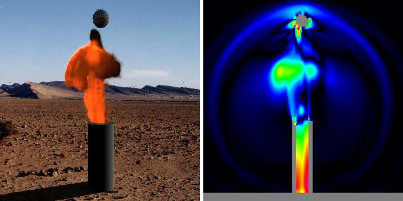
Figure 1: An image of a projectile propelled from a chamber by an explosion. On the right is a cross-section of the three-dimensional fluid volume using a colormap where hotter colors indicate higher densities.

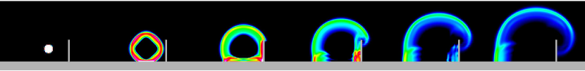
Figure 2: Shown here is a cross-section of pressures for a three-dimensional explosion near an immovable wall. The timestep between frames is 10 ms. Many of the behaviors of the blast wave can be seen, specifically the Mach stem formed from the blast wave merging with the wave reflected off the ground plane, and the diffracted wave formed when the blast wave crests over the wall.

Our fluid model of an explosion simulates many phenomena of blast waves that existing graphics techniques do not capture. Figure 2 shows a cross-section of pressures for a three-dimensional explosion near a wall. The initial disturbance in the first image interacts with the surrounding fluid and causes a pressure wave to propagate through the medium. In the second image, the blast wave has “shocked up,” as is evident by the large differences in pressure across the shock front. The blast wave reflects off the wall and the ground in the third image. In the fourth, the wave that reflected off the ground merges with the initial blast wave to form a Mach stem, which has pressure values twice that of the initial wave. In the final two images, the blast wave crests over the wall and forms a weaker diffracted wave.

In the entertainment industry, explosions are currently created at full scale in the real world, in miniature, or using heuristic graphics techniques[20, 9, 22]. Each of these methods has significant disadvantages, and we believe that in many scenarios, simulation may provide an easier solution. When explosions are generated and filmed at full scale in the real world, they often must be faked to appear dangerous and destructive by using multiple charges and chemicals with a low flashpoint. Because of the cost and danger of exploding full-size objects, many explosions are created using miniatures. With miniatures, the greatest challenge is often scaling the objects and the physics to create a realistic effect. Current graphics techniques for creating explosions are based on heuristics, analytical functions, or recorded data, and although they produce nice effects for spherical blast waves, they are not adequate for the complex effects required for many of the scenarios used in the entertainment industry.

Physically based simulations of explosions offer several potential advantages over these three techniques. In contrast to real physical explosions, simulations can be used in an iterative fashion, allowing the director many chances to modify or shape the effect. The rendering of the explosion is to a large extent decoupled from the simulation, allowing the visual characteristics of the dust clouds or fireball to be determined as a post-process. Unlike heuristic or analytical graphical methods, physically based simulations allow the computation of arbitrarily complex scenes with multiple interacting explosions and objects.

The next section discusses relevant previous work in explosions, fluids, flame, and fracture. The following section introduces the explosion model in the context of computational fluid dynamics. The next two sections discuss coupling between the fluid and solids and other secondary effects such as refraction and fireballs. We close with a discussion of our results.

2 Previous Work

Explosions used in the entertainment industry tend to be visually rich. Because of the inherent computational complexity of these explosions, researchers largely neglected this field after the publication of particle simulation techniques[16, 17]. Procedural methods can generate fiery, billowy clouds that could be used as explosions[3].

Recently two papers specifically addressed explosions. Mazarak and colleagues simulate the damage done by an explosion to voxelized objects[10]. They model the explosion as an ideal spherical blast wave with a pressure profile curve approximated by an analytic function based on the modified Friedlander equation and scaled according to empirical laws[2]. The spherical blast wave expands independent of existing obstacles, and forces are applied to objects in the direction of the blast radius. Objects are modeled as connected voxels and based on various heuristics, these radial forces may cause the voxels to disconnect.

Neff and Fiume use data from empirical blast curves to model an explosion[12]. The blast curves relate the pressure and velocity of the blast wave to time and are scalable. Unlike Mazarak and colleagues, they use a curve representing the reflection coefficient to apply forces to objects based on the angle of incidence of the blast wave. They assume quasi-static loading conditions where the blast wave encloses the entire object and effects due to reflected waves are ignored. They also model explosion-induced fracture in planar surfaces using a procedural pattern generator.

An alternative to these analytic and empirical models is a computational fluid dynamic simulation of the blast wave and the surrounding air. Foster and Metaxas presented a solution for incompressible, viscous flow and used it to animate liquids[5] and hot, turbulent gas[4]. They modeled fluid as a three-dimensional voxel volume with appropriate boundary conditions. The fluid obeys the Navier-Stokes equations; gas also follows an equation that represents thermal buoyancy. Using an explicit scheme, they update velocities and temperatures every timestep via Euler integration and readjust the values to guarantee conservation of mass. The fluid is rendered by tracing massless particles along the interpolated flow field. Their work with liquids included dynamic objects that were moved by the fluid, although they assumed that the objects were small enough not to influence the fluid. Recently Stam addressed the computational cost of guaranteeing stability by introducing extra damping to afford larger timesteps and using an implicit method to solve a sparse system of equations[18]. Stam’s method is inappropriate for shocks and explosions because his integration scheme achieves stability by encouraging the fluid to dissipate.

In the dramatic effects produced by the entertainment industry, a fireball is often the most salient visible characteristic of an explosion. Stam and Fiume modeled flame and the corresponding fluid flow and rendered the results using a sophisticated global illumination method[19]. The gases behaved according to advection-diffusion equations; Stam and Fiume solve these equations efficiently by reformulating the problem from a grid to “warped blobs.” Illumination from gas is affected by emission and anisotropic scattering and absorption. They only consider continuous emissions from blackbody radiation and ignore line emissions from electron excitation. They develop a heuristic for smoke emission due to the lack of a scientific analytic model.

Compressible flow has been studied for years in the computational fluid dynamics community[1, 2, 8]. We have built on this work by taking the governing equations and the donor-acceptor method of integration from this literature. However, the reasons for simulating explosions, combustion, detonation, and supersonic flow in engineering differ significantly from those in computer graphics. Engineering problems often require focusing on one element such as the boundary layer and simulating the other elements only to the extent that they affect the phenomenon under study. For example, engineering simulations are often two-dimensional and assume symmetry in the third dimension. Because they are focused on a specific event, their simulations may run for only a few microseconds. In computer graphics, on the other hand, we need to produce a visually appealing view of the behavior throughout the explosion. As a result, we need a more complete model with less quantitative accuracy.

3 Explosion Modeling

An explosion is a pressure wave caused by some initial disturbance, such as a detonation. In the results presented here, we assume that the detonation has occurred and that its properties are defined in the initial conditions of the simulation. This assumption is reasonable for most chemical explosions because the detonation is complete within microseconds. We animate explosions by modeling the pressure wave and the surrounding air as a fluid discretized over a three-dimensional rectilinear grid. The following two subsections describe the governing equations for fluid dynamics and the computational techniques used to solve them. The remaining two subsections describe the parameters available to the user for controlling the appearance of the explosion via the boundary conditions and initial conditions.

3.1 Fluid Dynamics

In nearly all engineering problems, including the analysis of explosions, fluids are modeled as a continuum. They are represented as a set of equations in terms of density $\rho$ ($\mbox{$\mathrm{kg}$}/\mbox{$\mathrm{m}$}^{3}$), pressure $P$ ($\mathrm{N}/\mathrm{m}^{2}$), velocity $v$ ($\mathrm{m}/\mathrm{s}$), temperature $T$ ($\mathrm{K}$), the internal energy per unit mass $N$ ($\mathrm{J}/\mathrm{kg}$), and the total energy per unit mass $E=N+\frac{1}{2}\mbox{\boldmath$v$}^{2}$ ($\mathrm{J}/\mathrm{kg}$). The equations that govern these quantities are defined in an Eulerian fashion, that is, they apply to a differential volume of space that is filled with fluid rather than to the fluid itself. In addition to the Navier-Stokes equations, which model the conservation of momentum, the equations for compressible, viscous flow include governing equations for the conservation of mass and energy and for the fluid’s thermodynamic state[7].

We introduce several simplifying assumptions that make the equations easier to compute but nevertheless allow us to capture the effects of compressible, viscous flow. We discount changes in the vibrational energies of molecules and assume air to be at chemical equilibrium; we ignore the effects from dissociation or ionization. These assumptions, which are commonly used in the engineering literature[1], allow us to reduce to constants many of the coefficients that vary with temperature. The resulting deviation in the values of the coefficients is negligible at temperatures below $1000\,\mbox{$\mathrm{K}$}$; only minor deviations occur below $2500\,\mbox{$\mathrm{K}$}$. Our implementation produces aesthetic results with temperatures above $100000,\mbox{$\mathrm{K}$}$, although deviations in constants could be on the order of a magnitude or two.

The first governing equation of fluid dynamics arises from the conservation of mass. Because fluid mass is conserved, the change of fluid density in a differential volume must be equal to the net flux across the volume’s boundary, giving

$$\frac{\partial\rho}{\partial t}=-\nabla\cdot(\rho{\mbox{\boldmath$v$}}).$$ (1)

The second governing equation, commonly known as the Navier-Stokes equation, concerns the conservation of momentum. For a Stokes fluid, where the normal stress is independent of the rate of dilation, the equation for the $x$ component of the fluid velocity is given by

$$\rho\frac{\partial\mbox{\boldmath$v$}_{x}}{\partial t}=\rho\mbox{\boldmath$f$}_{x}-\nabla P+\frac{\mu}{3}\nabla\cdot\left(\frac{\partial\mbox{\boldmath$v$}}{\partial x}\right)+\mu\nabla^{2}\mbox{\boldmath$v$}_{x}-\rho(\mbox{\boldmath$v$}\cdot\nabla)\mbox{\boldmath$v$}_{x},$$ (2)

where $f$ represents the body forces such as gravity and $\mu$ is the coefficient of viscosity. The equations for the $y$ and $z$ components are similar. The first two terms on the right-hand side of the equation model accelerations due to body forces and forces arising from the pressure gradient; the next two terms model accelerations due to viscous forces. The last term is not a force-related term; rather it is a convective term that models the transport of momentum as the fluid flows. This distinction between time derivative (force) terms and convective terms will be important for the integration scheme.

The final governing equation enforces the conservation of energy in the system. The First Law of Thermodynamics dictates that the change in energy is equal to the amount of heat added and the work done to the system. Accounting for the amount of work done from pressure and viscosity and the heat transferred from thermal conductivity yields

$$\rho\frac{\partial N}{\partial t}=k\nabla^{2}T-P\nabla\cdot\mbox{\boldmath$v$}+\Phi-\rho(\mbox{\boldmath$v$}\cdot\nabla)N,$$ (3)

where $k$ is the thermal conductivity constant and $\Phi$ is the viscous dissipation given by

$$\Phi=-\frac{2\mu}{3}(\nabla\cdot\mbox{\boldmath$v$})^{2}+\frac{\mu}{2}\sum_{i,j\in\{x,y,z\}}\left(\frac{\partial\mbox{\boldmath$v$}_{i}}{\partial j}+\frac{\partial\mbox{\boldmath$v$}_{j}}{\partial i}\right)^{2}.$$ (4)

As with equation (2), the last term of equation (3) is a convective term and models the transport of energy as the fluid flows.

In addition to the three governing equations, we need equations of state that determine the relationship between energy, temperature, density, and pressure. They are

$$N=c_{V}T,\;\;P=\rho RT,$$ (5)

where the coefficient $c_{V}$ is the specific heat at constant volume and $R$ is the gas constant of air.

Figure 3: Pressure profile ($\mathrm{N}/\mathrm{m}^{2}$) over time ($\mathrm{ms}$) near an explosion.

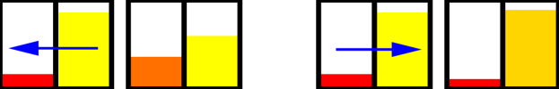
Figure 4: This figure illustrates the donor-acceptor method in which the amount of mass transferred is proportional to the mass of the donor. The voxels on the left show the transfer of mass and energy according to the flow, indicated by the blue arrow. The two voxels on the right represent the scenario with reversed flow of the same magnitude. Density is represented as height, and unit energy is represented as color. Corresponding amounts of energy are sent with the mass.

3.2 Discretization and Numerical Integration

The equations in the previous section describe the behavior of a fluid in a continuous fashion. However, implementing them in a form suitable for numerical computation requires that the space filled by the fluid be discretized in some manner and that a stable method for integrating the governing equations forward in time be devised.

Finite differences are used to discretize the space into a regular lattice of cubical cells. These finite voxels take the place of the differential volumes used to define the continuous equations, and the governing equations now hold for each voxel. Fluid properties such as pressure and velocity are associated with each voxel and these properties are assumed to be constant across the voxel. The spatial derivatives used in the governing equations are approximated on the lattice using central differences. For example, the $x$ component of the pressure gradient, $\nabla P$, at voxel $[i,j,k]$ is given by

$$\frac{\partial P}{\partial x}\approx\frac{P_{[i+1,j,k]}-P_{[i-1,j,k]}}{2h},$$ (6)

where subscripts in square brackets index voxel locations and $h$ is the voxel width.

After the governing equations have been expressed in terms of discrete variables using finite differences, they may be used as the update rules for an explicit integration scheme. However, rapid pressure changes created by steep pressure gradients moving at supersonic speeds would cause such a scheme to diverge rapidly. (See Figure 3.) To deal with this problem, we improved the basic integration technique using two modifications described in the fluid dynamics literature[2, 8]. The first modification involves updating equations (2) and (3) in two steps, first using only the temporal portion of the derivatives and second using the convective derivatives. The second modification is called the donor-acceptor method and is described in detail below. It addresses problems that arise when mass, momentum, and energy are convected across steep pressure gradients.

The modified update scheme operates by applying the following algorithm to each voxel at every timestep:

1. Approximate the fluid acceleration at the current time, $\mbox{\boldmath$\widetilde{a}$}_{t}=\left({\partial{\mbox{\boldmath$v$}}}/{\partial{t}}\right)_{t}$, using the non-convective (first four) terms of equation (2).

2. Compute the tentative velocity at the end of the timestep, $\mbox{\boldmath$\widetilde{v}$}_{t+\Delta t}=\mbox{\boldmath$v$}_{t}+\Delta t\mbox{\boldmath$\widetilde{a}$}_{t}$, and the approximate average velocity during the timestep $\mbox{\boldmath$\bar{v}$}_{t}=(\mbox{\boldmath$\widetilde{v}$}_{t+\Delta t}+\mbox{\boldmath$v$}_{t})/2$.

3. Approximate change in internal energy, $N$, using the non-convective terms of equation (3) and substituting $\mbox{\boldmath$\bar{v}$}_{t}$ for the fluid velocity.

4. Using $\mbox{\boldmath$\bar{v}$}_{t}$ for the fluid velocity, compute the new density, $\rho_{t+\Delta t}$ with equation (1).

5. Calculate the complete $\mbox{\boldmath${v}$}_{t+\Delta t}$ and $N_{t+\Delta t}$ with equations (2) and (3) using the convective terms and the new value of $\rho$.

6. Use state equations (5) to update secondary quantities such as temperature.

Although this update scheme is more stable than a simple Euler integration, sharp gradients in fluid density may still allow small flows from nearly empty voxels to generate negative fluid densities and cause inappropriately large changes to both velocity and internal energy. To prevent these problems, we use a donor-acceptor method when computing $-\nabla\rho\mbox{\boldmath$v$}$ of the convective terms in steps 4 and 5 above.

The donor-acceptor method transfers mass proportional to the mass of the voxel in the upstream direction, or donor voxel. Suppose we have voxel $i$ and one of its six neighbors $j$ in direction $d$ from $i$. Let $v_{ij}=\frac{1}{2}(\mbox{\boldmath$v$}_{i}+\mbox{\boldmath$v$}_{j})\cdot\mbox{\boldmath$d$}$. If $v_{ij}>0$, then flow is going from $i$ to $j$, $i$ is the donor, and $\rho_{i}$ is used in equation (1) to compute the change in voxel $i$’s density. Likewise, if $v_{ij}<0$, then $j$ is the donor, and the density of $j$ is used when computing the change in voxel $i$’s density. These calculations are repeated for the six neighbors of $i$ to obtain the new density for $i$, $\rho_{t+\Delta t}$. The velocity and energy convection are then scaled by ${\rho_{t}}/{\rho_{t+\Delta t}}$ to conserve momentum and energy. Figure 4 illustrates the donor-acceptor method. The left and right diagrams show flows in opposite directions of the same magnitude. The sent mass is proportional to the mass of the donor and carries with it corresponding amounts of energy.

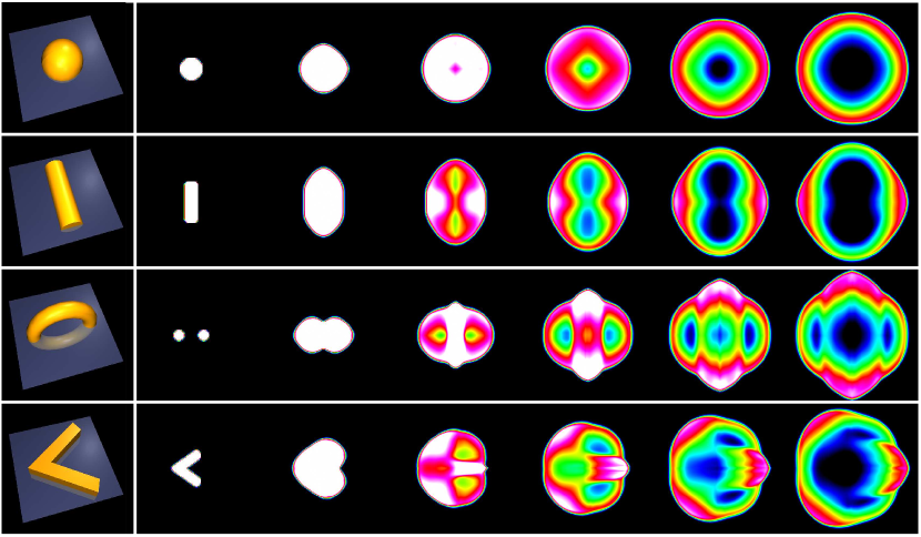
Figure 5: This figure shows cross-sections of pressure for three-dimensional explosions of equal-volume charges in the shape of a sphere, cylinder, torus, and wedge. The timestep between frames is 5 ms.

3.3 Boundary Conditions

The system has several types of boundary conditions that allow the fluid to exhibit a wide range of behaviors. Free boundaries allow blast waves to travel beyond the voxel volume as if the voxel volume were arbitrarily large. This type of boundary allows us to model slow, long-term aspects of explosions, such as fireballs and dust clouds. Hard boundaries force fluid velocity normal to them to be zero while leaving all other fluid attributes unchanged. We treat these boundaries as smooth surfaces, so tangential flow is unaffected. We implement a third boundary condition to achieve faster execution. If a voxel and its neighbors have pressure differences less than a threshold, the voxel is treated as a free boundary and is never evaluated. This optimization prunes out the majority of the volume while the blast wave is expanding.

3.4 Initial Conditions

The user specifies the pressure and temperature of the air, and the initial values of other variables are determined from the state equations (5). The detonation is initialized by specifying a region of the volume with higher temperature or pressure. For example, a chemical explosion might have a temperature of $2900\,\mbox{$\mathrm{K}$}$ and a pressure of $1000\,\mbox{$\mathrm{atm}$}$ with the surrounding air at $290\,\mbox{$\mathrm{K}$}$ and $1\,\mbox{$\mathrm{atm}$}$. The creation of the explosion may be time-delayed or may be triggered when the fluid around the charge reaches a threshold temperature.

The detonation may have an arbitrary geometry represented by a manifold polygonal mesh. The mesh is voxelized to initialize the appropriate voxels in the fluid simulation. By controlling the geometry, the user can produce a variety of effects that could not be achieved with a spherical model. In blast theory, planar, cylindrical, and spherical blast waves can be modeled by analytic functions[2]; however nonstandard shapes can create surprising and interesting effects. Figure 5 shows cross-sections of pressure for three-dimensional explosions from equal-volume charges in the shape of a sphere, cylinder, torus, and wedge. The inner blast wave of the torus merges to create a strong vertical blast wave. The wedge concentrates its force directly to the right, while leaving the surrounding area relatively untouched.

4 Interaction with Solids

People use explosions to impart forces on objects for both constructive and destructive purposes. The movements of these objects and the resulting displacement of air create many of the compelling visual effects of an explosion. In this section, we present methods to implement a two-way coupling between the fluid and solids. The coupling from fluid to solid allows us to model phenomena such as a projectile being propelled by an explosion. The coupling from solid to fluid can be used to model a piston compressing or the shock wave formed as a projectile moves through the air supersonically. We also extend previously published techniques for fracture to allow the pressure wave to shatter objects.

To allow the two-way coupling, objects have two representations: a polygonal mesh that is used to apply forces to the object from the fluid, and a volume representation in voxels that is used to displace fluid based on the motion of the object. We incorporate the coupling into the fluid dynamics code in the following way:

1. Apply forces on the objects from the fluid and compute the rigid body motion of the objects.

2. If the object has moved more than a fraction of a voxel, recompute the voxelization of the object.

3. Displace fluid based on object movement.

4. Update the fluid using the techniques described in Section 3.2.

We explain the first three of these items in greater detail in the following subsections.

4.1 Coupling from Fluid to Solid

An object embedded in a fluid experiences two separate sets of forces on its surface, those arising from hydrostatic pressure and those arising from dynamic forces due to fluid momentum. The forces due to hydrostatic pressure act normal to the surface and are generated by the incoherent motions of the fluid molecules against the surface. The dynamic forces are generated by the coherent motion of the continuous fluid and can be divided into a force normal to the surface of the object and a tangential shearing force. We neglect the tangential shearing force because in the context of explosions, it is negligible in comparison to the force due to hydrostatic pressure. We assume that the object is in equilibrium under ambient air pressure and the hydrostatic forces are computed using the overpressure $\bar{P}$, which is the difference between the hydrostatic pressure $P$ and ambient pressure.

The magnitude of the normal force per unit area on the surface is given by the dynamic overpressure:

$$\bar{P}_{\mathit{dyn}}=\bar{P}+\frac{1}{2}\rho\left(\mbox{\boldmath$v$}_{\mathit{rel}}\cdot\mbox{\boldmath$\hat{n}$}\right)^{2},$$ (7)

where $\mbox{\boldmath$v$}_{\mathit{rel}}$ is the velocity of the fluid relative to the surface, and $\hat{n}$ is the outward surface normal.

We assume that the triangles composing each object are small enough that the force is constant over each triangle. The force on a triangle with area $A$ is then

$$\mbox{\boldmath$f$}=-\mbox{\boldmath$\hat{n}$}A\bar{P}_{\mathit{dyn}},$$ (8)

where the fluid properties are measured at the centroid of the triangle. The forces are computed for all triangles of an object, and the translational and angular velocities of the object are updated accordingly.

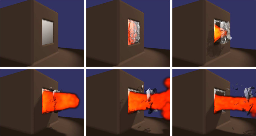
Figure 6: A glass window is shattered by a blast wave. The blast wave pressure is approximately $3\,\mbox{$\mathrm{atm}$}$ when it reaches the window. The images show the scene at 0 ms, 13 ms, 40 ms, 67 ms, 107 ms, and 160 ms.

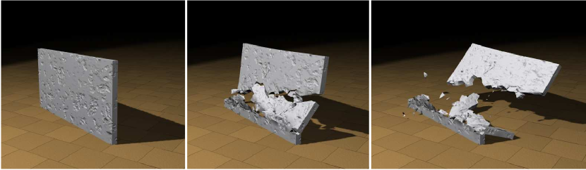
Figure 7: A wall is knocked over by a blast wave from an explosion 3.5 m away. The images are spaced 250 ms apart.

In addition to acting on rigid objects, the forces can also be applied to flexible objects that deform and fracture[14]. The explosion simulation results in pressures, velocities, and densities for each voxel in the discretization of the fluid. The fracture simulation uses this information to compute the forces that should be applied to a finite element model of the objects in the scene. The force computation is similar to that for rigid objects. This method was used to simulate the breaking window shown in Figure 6 and the breaking wall shown in Figure 7. This coupling is one-way in that the fluid applies forces to the finite-element model, but the fluid is not moved by the fragments that pass through it.

4.2 Coupling from Solid to Fluid

To allow the solid to displace fluid, the triangular mesh representing the object is converted to voxels[13], which are then used to define the hard boundaries in the fluid volume dynamically. The objects move smoothly through the fluid, but because of the discrete nature of the voxelization, large changes in the amount of fluid displaced may occur on each timestep. To address this problem, the fluid displaced or the void created by the movement of the objects is handled over a period of time rather than instantaneously.

The voxelization returns a value between zero and one representing the proportion of the voxel that is not interior to any object. This value is independent of geometric considerations about the exact shape of the occupied volume. If any dimension of an object is smaller than the size of a voxel, the appropriate voxels will have partial volumes, but because there are no fully occupied voxels, the fluid will appear to move through the object. Nonzero partial volumes below a certain threshold are set to zero to increase stability. The implementation of partial volumes requires slight modifications to the donor-acceptor method to conserve mass, momentum, and energy because two adjacent voxels could have different volumes.

When any part of an object moves more than a fraction of a voxel, the object is revoxelized, and the hard boundaries of the fluid are updated. When this process occurs, the partial volume in a voxel might change, resulting in fluid flow. We allow this flow to occur smoothly by sacrificing conservation of mass and energy in the short-term. The voxelization determines the partial volumes in an instantaneous fashion, but the fluid displacement routine maintains internal partial volumes that change more slowly and are used to compute the pressure, density, and temperature of the affected voxels. The internal partial volumes change proportionally to the velocities of the moving objects, and mass and energy are restored over time.

To compute a smooth change in the internal partial volume from $V_{1}$ to $V_{2}$, we model an object moving into a voxel as a piston compressing or decompressing fluid. We simplify the computation of the change in partial volume by assuming that the piston is acting along one of the axes of the voxelization. The appropriate axis is selected based on the largest axial component of the velocity of the object, $\mbox{\boldmath$v$}_{p}$. The displacement of the piston after $t$ seconds and the corresponding change in partial volume of a voxel with width $h$ are

$$\mbox{\boldmath$l$}=\mbox{\boldmath$v$}_{p}t,\;\;\Delta V=V_{2}-V_{1}=h^{2}\mbox{\boldmath$v$}_{p}t.$$ (9)

The displacement occurs linearly over

$$t={\Delta V\over h^{2}\mbox{\boldmath$v_{p}$}}$$ (10)

at a velocity of $\mbox{\boldmath$v$}_{p}$.

Given this model of the change in internal partial volume, we know that $\rho_{1}V_{1}=\rho_{2}V_{2}$ because mass is conserved. However, the fluid is compressible, so mechanical energy is not conserved (otherwise $P_{1}V_{1}=P_{2}V_{2}$). To obtain the new pressures and densities of the fluid, we use a thermodynamic equation relating the work done to the system from changing the volume (or density),

$$\frac{P_{2}}{P_{1}}=\left(\frac{\rho_{2}}{\rho_{1}}\right)^{\gamma}=\left(\frac{T_{2}}{T_{1}}\right)^{\gamma/(\gamma-1)},$$ (11)

where $\gamma=1+R/c_{V}$ ($\gamma$ is about 1.4 for air and is closer to 1 the more incompressible the fluid)[1]. Internal unit energy and total unit energy are then updated by the state equations.

When the partial volume of a voxel changes from one nonzero value to another, the resulting pressure changes cause fluid to move to or from a neighbor based on the governing equations. However, when the partial volume of a voxel changes from zero to nonzero or vice versa, the situation must be handled as a special case by treating the affected voxel and one of its neighbors as a single larger voxel with a nonzero partial volume. The neighbor is selected based on the largest axial component of the object’s velocity, $\mbox{\boldmath$v$}_{p}$. We calculate the internal partial volume for each of the involved voxels $A$ and $B$ as $\widetilde{V}_{A_{1}}$ and $\widetilde{V}_{B_{1}}$.

When $V_{A_{1}}$, the original partial volume of $A$, is zero and $V_{A_{2}}$, the new partial volume of $A$, is nonzero, we use initial volumes $\widetilde{V}_{A_{1}}$ and $\widetilde{V}_{B_{1}}$ such that $\widetilde{V}_{A_{1}}+\widetilde{V}_{B_{1}}=V_{B_{1}}$ (the initial volume is conserved) and $\widetilde{V}_{A_{1}}{V}_{B_{2}}=\widetilde{V}_{B_{1}}V_{A_{2}}$ (the voxels are treated as a single larger voxel). The change in volume is

$$\Delta{V}_{A} = {V}_{A_{2}}-\widetilde{V}_{A_{1}}={V}_{A_{2}}-{V}_{A_{2}}\frac{V_{B_{1}}}{{V}_{A_{2}}+{V}_{B_{2}}},$$ (12)

$$\Delta{V}_{B} = {V}_{B_{2}}-\widetilde{V}_{B_{1}}={V}_{B_{2}}-{V}_{B_{2}}\frac{V_{B_{1}}}{{V}_{A_{2}}+{V}_{B_{2}}}.$$ (13)

When the original partial volume of $A$, $V_{A_{1}}$, is nonzero and the new partial volume of $A$, $V_{A_{2}}$, is zero, we force $\widetilde{V}_{A_{1}}$ to be zero and treat $\widetilde{V}_{B_{1}}$ as a single larger voxel. To treat the two voxels as one, we first average the properties of $A$ and its neighbor $B$, transferring any lost kinetic energy to internal energy. The change in volume is then

$$\Delta{V}_{B}=V_{B_{2}}-\widetilde{V}_{B_{1}}=V_{B_{2}}-{\rho_{A}{V}_{A_{1}}+\rho_{B}{V}_{B_{1}}\over\rho_{B}}$$ (14)

by making sure that $\rho_{B}\widetilde{V}_{B_{1}}=\rho_{A}V_{A_{1}}+\rho_{B}V_{B_{1}}$ (mass is conserved).

5 Secondary Effects

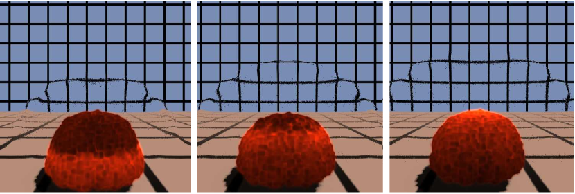
Figure 8: Refraction of light from a blast wave. Each frame is 10 ms apart. The index of refraction is exaggerated tenfold to enhance the effect.

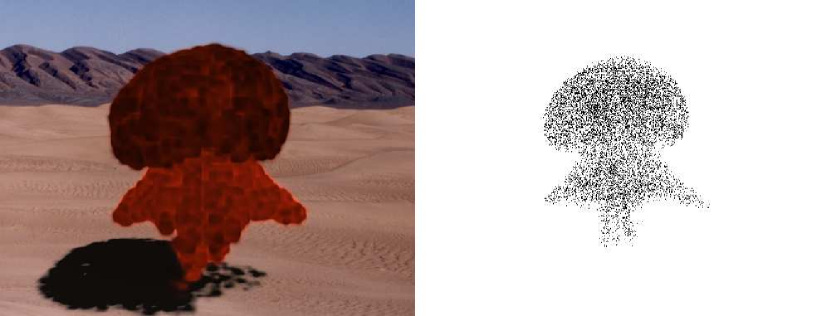
Figure 9: A fireball after one second of simulation time. Tracer particles from the fluid simulation determine the position and coloration of the fireball.

An explosion creates a number of visual secondary effects including the refraction of light, fireballs, and dust clouds. These secondary effects do not significantly affect the simulation, so they can be generated and edited as a post-process.

One of the most stunning, but often ignored, effects of an explosion is the bending of light from the blast wave. Because the blast wave is substantially denser than the surrounding air, it has a higher index of refraction, $\eta$. Light travels at the same velocity between molecules, but near molecules it is slowed down from interactions with electrons. This concept is expressed numerically as $\eta-1=k\rho,\;k=2.26\times 10^{-4}\;\mathrm{m}^{3}/\mathrm{kg}$, by the Dale-Gladestone law[11]. We capture the refraction of light by ray tracing through the fluid volume. (See Figure 8.) As the ray is traced through the volume, the index of refraction is continually updated based on the interpolated density of the current position. For simplicity, we compute the density of each point using a trilinear interpolation of the densities of the neighboring voxels. When the index of refraction changes by more than a threshold, the new direction of the ray is computed via Snell’s law using the density gradient as the surface normal. The trilinear interpolation results in minor faceting effects that cause small errors in the reflected direction.

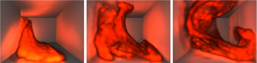
Figure 10: A fireball coming around a corner. The images are spaced 333 ms apart.

An advantage of using a full volumetric fluid representation for explosions is that the simulation can be used to model a fireball in addition to the blast wave. We assume that the fireball is composed of detonated material from inside the explosive. To track this material, the system initializes the fireball by placing particles inside the shape specified by the user for the explosion. The particles are massless and flow with the fluid, allowing the fluid dynamics model to capture effects critical for a fireball such as thermal conductivity and buoyancy. Some fluid simulations[4, 18] model thermal buoyancy explicitly; in our simulation, thermal buoyancy is a behavior derived from the governing equations. For rendering, each particle takes on a temperature that is interpolated based on its position in the volume. The particles are rendered as Gaussian blobs with values for red, green, blue, and opacity. The color values are based on blackbody radiation at appropriate wavelengths given the temperature of the particle[11]. Figure 9 shows a fireball and corresponding tracer particles after one second of simulation. Figure 10 shows a fireball coming around a corner; the hallway is illuminated by the flames.

The tracer particles couple the appearance of the fireball to the motion of the fluid, and although heat generated by the initial explosion is added to the fluid model, any additional heat generated by post-detonation combustion is ignored. Radiative energy released at detonation could also be modeled for rendering. Much like the difficulties encountered with rendering the sun[15], the high contrast of this effect may require contrast-reduction techniques such as LCIS[21].

The blast wave and other secondary waves create dust clouds by disturbing fine particles resting on surfaces. The creation of dust clouds is difficult to quantify either experimentally or analytically, so the rate at which the dust becomes airborne is left as a control for the animator. Once a dust particle is airborne, its behavior is dictated by its size. The smaller it is, the more it is influenced by drag forces and the less it is influenced by inertial forces. Smaller dust particles have lower terminal velocities and exhibit more Brownian motion. With the exception of coagulated particles, experiments reveal that most dust particles are approximately ellipsoidal with low eccentricity, and the particles do not orient themselves to the fluid flow[6]. The difference in dynamics between these particles and spherical particles is not that significant, so we assume dust particles to be spherical. We implement dust as metaparticles, each representing a Gaussian density of homogeneous dust particles. The dust size for each metaparticle is chosen according to size distributions from experimental data for blasted shale[6]. The metaparticles travel through the fluid as if single particles were located at their centers. Their variances grow according to the mean Brownian diffusion per unit time. Figure 11 shows dust clouds in a city scene.

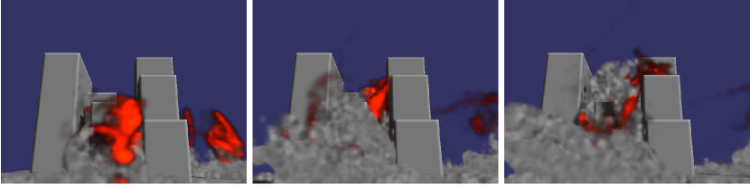
Figure 11: An explosion among buildings. The images are spaced 667 ms apart.

6 Results and Discussion

We ran the system with several scenarios. The physical constants used in the simulation were constants for air that were taken from an engineering handbook[7]. Table 1 shows the voxel width, timestep, total simulation time, initial volume of the explosion (proportional to yield), and initial pressure and temperature of the explosion. The timesteps $\Delta t$ increase by a factor of five once the blast wave leaves the volume.

The simulations ran on a single 195 MHz R10K processor and used a $101\times 101\times 101$ volume. The running times per timestep varied considerably from several seconds to two minutes because of the pruning described in Section 3.3. For coupling with fracture, I/O became a major factor because in each iteration the entire volume was written to disk; however, using better compression would reduce this expense. Running times of the simulations varied from a few hours (Figure 5) to overnight (Figures 2, 6, 7, and 8) to a few days (Figures 1, 9, 10, and 12).

Example	$h$	$\Delta t$	$t_{tot}$	$V_{0}$	$P_{0}$	$T_{0}$
(figure)	($\mathrm{m}$)	($\mathrm{ms}$)	($\mathrm{ms}$)	($\mathrm{m}^{3}$)	($\mathrm{atm}$)	($\mathrm{K}$)
projectile (1)	1.0	0.10	450	73.60	1000	2900
barrier (2)	0.2	0.01	25	0.52	1000	2900
shapes (5)	1.0	0.10	30	1000.00	1000	2900
fracture (6,7)	0.2	0.02	20	0.52	1000	2900
fireball (8,9)	1.0	0.10	1000	65.40	1000	2900
corner (10)	1.0	0.10	10000	268.08	1000	2900
city (11)	1.0	0.10	5000	65.40	1000	2900
nuclear (12)	50.0	0.50	30000	$\mathsf{9.1}\!\!\times\!\!\mathsf{10}^{\mathsf{7}}$	345	$\mathsf{1}\!\!\times\!\!\mathsf{10}^{\mathsf{5}}$

Table 1: Parameters for simulations: voxel width, timestep, total simulation time, and initial volume, pressure, and temperature of detonation.

We use an explicit integration technique to compute the motion of the pressure wave caused by the detonation. Despite its magnitude, the wave does not transport fluid large distances. Previously, fluid dynamics has been used most often in computer graphics to capture the effects of macroscale fluid transport where the fluid does move a significant distance. Implicit integration techniques with large timesteps are appropriate for these situations because they achieve stability by damping high frequencies. The propagation of the pressure wave in our stiff equations, however, is characterized by these high frequencies and it is essential that they not be artificially damped. We chose, therefore, to use an explicit integration technique; however, an implicit integration technique could be used to simulate the fireball and dust clouds after the blast wave and the secondary waves have left the volume. Using an implicit integration technique in the slow flow regime could allow larger timesteps and faster execution times.

We assume that the voxels in the fluid volume are of a size appropriate for the phenomena that we wish to capture. In particular, if solid objects have a dimension smaller than a voxel, then they will not create a hard boundary that prevents fluid flow. For example, a wall that is thinner than a voxel will permit the blast wave to travel through it because partial volumes do not maintain any geometric information about the sub-voxel shape of the object. The difficulty of a two-way coupling with fracturing objects stems from having to model subvoxel cracks, which should allow flow to go through. If small objects are required, the voxel size could be decreased or dynamic remeshing techniques could be used to create smaller voxels in the areas around boundaries.

There are effects from explosions that we have not investigated. Although smoke is often a visible feature of an explosion that includes a fireball, we do not have a physically based model for smoke creation. Incomplete combustion at lower temperatures results in smoke, and that observation could be used as a heuristic to determine where smoke should be created in the fireball and how densely. Stam and Fiume used a similar heuristic model[19]. Textures of objects could be modified to show soot accumulation and scorching over time. Dust clouds are created when an object fractures or pulverizes. Dust could be introduced into our system when the finite-element model produces small tetrahedra or when cracks form.

We made several assumptions in constructing our model of explosions. Most discounted effects that did not contribute noticeably to the final rendered images; however, some could produce a noticeable change in behavior in certain situations and may warrant further investigation. We only model the blast wave traveling through air. However, waves travel through other media, including solid objects, and complex interface effects occur when a wave travels between two different media. For large-scale explosions, meteorological conditions such as the change in pressure with respect to altitude or the interface between atmospheric layers (the tropopause) may need to be considered.

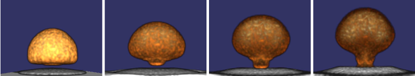
Figure 12: A large-scale high-temperature explosion resembling a nuclear explosion: after 3 s, 6 s, 12 s, 24 s.

Our goal in this work has been to create a physically realistic model of explosions. However, this model should also lend itself to creating less realistic effects. Even though our model does not incorporate high-temperature effects such as ionization, we can still obtain interesting results on high-temperature explosions. The fireball in Figure 12 resulted from an initial detonation at $10^{5}\,K$. Explosions used in feature films often include far more dramatic fireballs than would occur in the actual explosions that they purport to mimic. By using more tracer particles and adjusting the rendering parameters of the fireballs, we should be able to reproduce this effect. Noise could be added either to the velocity fields or particle positions post-process to make the explosion look more turbulent. Similarly, explosions in space are often portrayed as more colorful and violent than explosions that occurred outside of the atmosphere should be. Imparting an initial outward velocity to the explosion, turning off gravity, and increasing the thermal buoyancy by modifying the state equations might create a similar effect.

7 Acknowledgments

This project was supported in part by NSF NYI Grant No. IRI-9457621, Mitsubishi Electric Research Laboratory, and a Packard Fellowship. The second author was supported by a Fellowship from the Intel Foundation.

References

- [1] J. D. Anderson Jr. Modern compressible flow: with historical perspective. McGraw-Hill, Inc., 1990.
- [2] W. E. Baker. Explosions in air. University of Texas Press, 1973.
- [3] D. Ebert, K. Musgrave, D. Peachy, K. Perlin, and S. Worley. Texturing and Modeling: A Procedural Approach. AP Professional, 1994.
- [4] N. Foster and D. Metaxas. Modeling the motion of a hot, turbulent gas. Proceedings of SIGGRAPH 97, pages 181–188, August 1997.
- [5] N. Foster and D. Metaxas. Realistic animation of liquids. Graphics Interface ’96, pages 204–212, May 1996.
- [6] H. L. Green and W. R. Lane. Particulate Clouds: Dusts, Smokes and Mists. D. Van Nostrand Company, Inc., 1964.
- [7] A. M. Kuethe and C. Chow. Foundations of aerodynamics: bases of aerodynamic design. John Wiley and Sons, Inc., 1998.
- [8] C. L. Madder. Numerical modeling of detonations. University of California Press, 1979.
- [9] K. H. Martin. Godzilla: The sound and the fury. Cinefex, pages 82–107, July 1998.
- [10] O. Mazarak, C. Martins, and J. Amanatides. Animating exploding objects. Graphics Interface ’99, pages 211–218, June 1999.
- [11] J. R. Meyer-Arendt. Introduction to classical and modern optics. Prentice-Hall, Inc., 1984.
- [12] M. Neff and E. Fiume. A visual model for blast waves and fracture. Graphics Interface ’99, pages 193–202, June 1999.
- [13] F.S. Nooruddin and G. Turk. Simplification and repair of polygonal models using volumetric techniques. Technical Report GIT-GVU-99-37, Georgia Institute of Technology, 1999.
- [14] J. F. O’Brien and J. K. Hodgins. Graphical modeling and animation of brittle fracture. Proceedings of SIGGRAPH 99, pages 137–146, August 1999.
- [15] A. J. Preetham, P. Shirley, and B. E. Smits. A practical analytic model for daylight. Proceedings of SIGGRAPH 99, pages 91–100, August 1999.
- [16] W. T. Reeves. Particle systems—a technique for modeling a class of fuzzy objects. ACM Transactions on Graphics, 2(2):91–108, April 1983.
- [17] K. Sims. Particle animation and rendering using data parallel computation. Computer Graphics (Proceedings of SIGGRAPH 90), 24(4):405–413, August 1990.
- [18] J. Stam. Stable fluids. Proceedings of SIGGRAPH 99, pages 121–128, August 1999.
- [19] J. Stam and E. Fiume. Depicting fire and other gaseous phenomena using diffusion processes. Proceedings of SIGGRAPH 95, pages 129–136, August 1995.
- [20] R. Street. Volcano: Toasting the coast. Cinefex, pages 56–84, September 1997.
- [21] J. Tumblin and G. Turk. LCIS: A boundary hierarchy for detail-preserving contrast reduction. Proceedings of SIGGRAPH 99, pages 83–90, August 1999.
- [22] M. C. Vaz. Journey to Armageddon. Cinefex, pages 68–93, October 1998.