ABSTRACT

This is the open-print version of my dissertation thesis in 2014 [1]. In this open-print version, several Figures were inevitably eliminated, because of the copyright and/or file-size problems. Those figures are indicated with the message “(Figure is hidden in open-print version.)”, whereas original files could be available from T. OISHI when requested. Several minor corrections have been also done, but without changing the scientific discussions, results, and conclusions from the original version [1].

In this thesis, I investigate the two-proton emission in proton-rich nuclei. The aim of study is to discuss the relation between the observables of this emission and the diproton correlation with quantum entanglement, which is one characteristic phenomenon due to the nuclear pairing interaction.

The pairing correlation between two nucleons plays an essential role in nuclear structure. Especially, two nucleons near the Fermi surface in nuclei have been predicted to make the “diproton” and “dineutron” correlations. These correlations mean the spatial localization of two nucleons, associated with the dominance of the spin-singlet configuration with entanglement. Especially, the dineutron correlation has been actively studied recently with a strong connection to the exotic features of neutron-rich nuclei. These nuclei far from the beta-stability line have attracted novel interests in nuclear physics, and their basic information have been extensively investigated for the past few decades. On the other hand, the diproton correlation in proton-rich nuclei has been less studied.

In the former half of this thesis, I discuss the universality of the diproton and dineutron correlations, with a theoretical study of the ^17,18Ne and ¹⁸O nuclei. This study is based on a three-body model, which provides a semi-microscopic description for the two nucleons inside nuclei. I demonstrate that a diproton correlation exists in the ground state of ^17,18Ne, similarly to a dineutron correlation in ¹⁸O. It is also shown that the Coulomb repulsive force between the two protons does not affect significantly this correlation. Consequently, the nuclear pairing interaction plays an important role to occur the dinucleon correlations inside nuclei.

The later half of this thesis focuses on the relation between the diproton correlation and the two-proton emission. Even with theoretical predictions, for the dinucleon correlations, there have been no direct experimental evidences, because of a difficulty to access the intrinsic structures of nuclei. Recently, on the other hand, “two-proton emission” has been focused as a direct probe into the diproton correlation with entanglement. Namely, via this process, a pair of protons is emitted directly from the parent nuclei. The emitted two protons are expected to provide information about the nuclear pairing interaction and the diproton correlation. In order to extract such information, one has to consider both the quantum meta-stability and the many-body properties in an unified framework. For this purpose, I develop a time-dependent three-body model. By applying this model to the ⁶Be nucleus, which is the lightest two-proton emitter, I investigate several novel properties about the role of pairing correlations in the meta-stable state. It has been shown that, by considering the Cooper pairing in the initial state of the two protons, (i) the experimental decay width of ⁶Be is well reproduced, and (ii) the two protons are emitted mainly as a diproton-like cluster with the spin-singlet configuration, in the early stage of the emission. These results strongly suggest the diproton correlation during the emission process. Namely, the two-proton emission can be an efficient tool to access the diproton correlation with a strong entanglement.

Despite these important theoretical findings, in order to extract the information on the diproton correlation from the experimental data, there still remain several points to be improved. The most important one is to take the final-state interactions into account sufficiently. For the two-proton emission from the ⁶Be nucleus, my result for the early stage of the emission predicts a dominant diproton-like configuration. On the other hand, there is only little signal of such a configuration in the experimental data of the energy-angular correlation pattern, which correspond to the late stage of the emission. This discrepancy is due to a strong disruption of the diproton correlation in the late stage, caused by the final-state interactions among all the particles. In order to establish the agreement between the calculated result and the experimental data, I need to expand the model-space so that a longer time-evolution can be carried out.

As a summary of this thesis, the first step to investigate the diproton correlation by means of the two-proton emission has been established. The time-dependent method based on the three-body model has provided an intuitive way to describe the quantum dynamics of the entangled fermionic pair, with an advantage to understand the role of pairing correlations. I expect that the improved time-dependent method will be a powerful tool for two-proton emissions, and also for other quantum meta-stable processes. After further investigations, the obtained knowledge of the pairing correlations and the meta-stable processes will be an important result not only for nuclear physics but also for atomic, molecular, condensed matter and quantum informative physics.

Chapter 1 Introduction

Pairing correlations are characteristic phenomena in many-fermion systems. Especially, the nuclear pairing correlation has been a major subject of modern nuclear physics [2, 3, 4, 5, 6, 7]. After the establishment of the traditional mean-field theory for atomic nuclei, there have been enormous theoretical, experimental and computational developments in this field. These developments have led to a deeper insight beyond the pure mean-field picture.

Within the traditional mean-field theory, any nucleon inside a nucleus is assumed to be an independent particle moving in the mean-field generated by the interactions among all the nucleons. The traditional mean-field theory was applied to atomic nuclei, e.g. by Mayer et.al. [8, 9], leading to conclusions about the shell structures and the magic numbers, which excellently agree with empirical properties of atomic nuclei. A more sophisticated definition of the nuclear mean-field is given by applying the Hartree-Fock (HF) theory [10, 11, 12, 13] . Within the HF theory, the mean-field for an arbitrary nucleon is defined self-consistently by considering effective nucleon-nucleon interactions from all the other nucleons . However, this traditional mean-field theory takes into account the interaction only on average, and thus misses some parts of the interaction, which is called the “residual interaction”.

The “pairing interaction” is the most important part of the residual interaction. Taking the pairing interaction into account, the traditional mean-field picture is modified to that including a collection of two correlated nucleons. two nucleons, which are in unnegligible correlations. The pairing interaction brings about a significant attraction between two nucleons when those are coupled to be the spin-singlet state [5, 13]. Evidences for the pairing correlations can be found, for instance, in the fact that there is a universal odd-even staggering rule in the binding energies. That is, even-even nuclei are systematically more bound than the neighboring nuclei in the nuclear chart. It is also known that the even-even nuclei take the spin-parity of $0^{+}$ in the ground state, with no exceptions. Similar pairing correlations play important a role not only in nuclei, but also in several other systems including condensed matters and cold fermionic atoms.

In recent years, the study of nuclear pairing interactions and correlations has gained a renewed interest, due to the progress of physics of “unstable nuclei” [6, 7, 14]. Unstable nuclei, which have large neutron- or proton-excess and locate far from the $\beta$-stability line, have been a major topic in recent nuclear physics. For these nuclei, there are considerably novel features which can be connected to the pairing correlation [14]. Those include “dinucleon correlation”, which we detail in the next section.

1.1 Dinucleon Correlation

The diproton and the dineutron correlations are intrinsic structural properties of atomic nuclei, caused by the pairing interaction. As is well known, a diproton or a dineutron is not bound in the vacuum, where the only possible bound state of two nucleons is a deuteron. However, inside nuclei, the situation may be different from that in the vacuum. Because of the many-body effect on pairing correlations, a possibility of the existence of diproton and dineutron-like configurations has been discussed for more than 40 years, since the first proposal by Migdal in 1973 [15]. These phenomena are called “dinucleon correlations”. The study of dinucleon correlations is expected to provide a novel and universal insight into other strongly-correlated many-fermion systems.

Based on the microscopic theory for the pairing correlations, e.g. HF-Bardeen-Cooper-Schrieffer (HF-BCS) or HF-Bogoliubov (HFB) theory [13, 6, 7], it has been known that the pairing correlation depends on the surrounding density, $\rho$ [16, 17, 18, 19, 20, 21]. For instance, the pairing gap in infinite nuclear matter takes the maximum at a density smaller than the normal density. This density-dependence is naively due to the many-fermion effects. However, the exact origin of this density-dependence has remained unclarified, though some candidates have been discussed. Those include (i) the momentum-dependence of bare nucleon-nucleon forces, (ii) the Pauli principle and (iii) effects of nuclear three-body forces. It should be emphasized that this density-dependence causes a variety of pairing correlations. In the deeper region of nuclei with normal nuclear matter-density, a pair of nucleons is found to be a Cooper pair in the HF-BCS theory [5]. This pair is in the regime of weak pairing correlations, and its spatial distribution is much expanded compared to the typical radii of nuclei. On the other hand, in the low density region, the situation can be altered due to the density-dependence of the pairing correlation. The effective pairing correlation can be enhanced in that region, resulting in the spatial localization of two neutrons and protons, and also the increase of the probability of the spin-singlet configuration. Namely, in this situation, a pair of nucleons plays as a dineutron- or diproton-like cluster. The existence of this strong correlation can be considered within a wide range of the surrounding density, $\rho/\rho_{0}\sim 0.1-0.01$, where $\rho_{0}\sim 0.15$ fm^-3 is the nuclear saturation density [18]. Finally, if the density becomes infinitesimally small, the pairing correlation vanishes and two neutrons or protons become unbound. This limit is identical to two nucleons in the vacuum.

From a phenomenological point of view, the dinucleon correlation is a kind of phase-crossover in many-nucleon systems with dilute densities . Such a dilute density-situation has been expected to occur especially in the valence orbits of weakly-bound neutron-rich nuclei. For the past about two decades, neutron-rich nuclei with large neutron-excess and shorter lifetimes for the beta-decay have been extensively studied. This is grealy thanks to the experimental achievements which have provided the access to these nuclei [23, 24]. In the ground state of these nuclei, the valence neutrons should be in the outer orbit far from the core, where the surrounding density is not so large that the pairing correlation is expected to increase [16, 17]. This is especially the case for weakly bound nucleons [25, 26, 27, 28]. Various theoretical and experimental studies have been performed to investigate the dineutron-correlation in such nuclei, in connection to its influence on the nuclear structures and reactions. These studies have shown that the correlation may invoke sizable effects on some phenomena, including the electro-magnetic excitations [29, 27, 30], the Coulomb break-up reactions [31, 32, 33, 34, 35, 36] and the pair-transfer reactions [37, 38, 39]. On the other hand, for proton-rich nuclei, even though a similar diproton correlation can be considered [40], it has so far been less studied compared to the dineutron correlation. Whether the Coulomb repulsion disrupts the diproton-like configuration or not in proton-rich nuclei is still an remaining question, though its effect has been found to be weak compared to the nuclear attraction [40, 41, 42, 43, 44]. For both dineutron and diproton correlations, further quantitative and qualitative investigations are still in progress today.

The prediction of the dinucleon correlation is an important conclusion from the recent nuclear theory, and its detection will give us a strong constraint on the basic properties of our nuclear models. However, as we will discuss in Chapter 2, even with various efforts, there have been no direct experimental evidences for the dinucleon correlation, mainly because it is an intrinsic structure which is hard to be detected.

1.2 Two-Proton Decay and Emission

Given these difficulties mentioned in the previous section, “two-proton emission” and “two-proton radioactive decay” have been expected to provide a novel way to access the diproton correlation. Those are the quantum tunneling phenomena that two protons are emitted from the proton-rich nuclei beyond the proton-dripline [45, 46, 47]. In this process, the decay products can be strongly associated with the pairing correlation between two protons. The importance of pairing correlations are suggested from, for instance, that observed 2p-emitters have the even number of protons with no exceptions. Thus, emitted two protons are expected to carry information about the pairing correlations, probably including the diproton correlations in nuclei [48, 49]. We focus on these phenomena in the next section.

The oldest example of the two-proton (2p-) emitter is the ⁶Be nucleus, where its “alpha+p+p” resonance has been experimentally observed for several decades [50, 51, 52, 53, 54, 55, 56, 57]. Following ⁶Be, similar three-body resonances have been observed in the ground state of a few light proton-rich nuclei, such as ¹²O [58, 59] and ¹⁶Ne [58, 60]. A typical Q-value and decay-width of these resonances are on the order of 100 keV. For these nuclei, the potential barrier between the core and a proton is mainly due to the centrifugal force, whereas the Coulomb force is relatively small. Because of the low potential barrier, the decay width is comparably broad compared to the Q-value of these nuclei.

On the other hand, the 2p-radioactive decay is a novel decay-mode of medium-heavy and heavy nuclei outside the proton-dripline . A typical lifetime for the 2p-decays of these nuclei is 1-10 ms, corresponding to a typical decay width of $10^{-18}$-$10^{-19}$ MeV. A typical Q-value is around 1 MeV, similarly to light 2p-emitters. The significantly narrow width, compared with light 2p-emitters, is due to the higher Coulomb barriers, which considerably reduce the tunneling probabilities of two protons. In this category, ⁴⁵Fe is the most famous example for the 2p-radioactivity. At the beginning of 2000s, the first observation of 2p-radioactivity was made for the ⁴⁵Fe nucleus [62, 63]. After this first discovery, the 2p-radioactivity has been confirmed also for ⁵⁴Zn and possibly for ⁴⁸Ni.

It is also predicted that the 2p-decays and emissions are not limited particularly in these nuclides but universally exist along the proton-dripline until $Z\leq 82$ [47, 61]. Suggested nuclides to have this decay-mode include ${}^{26}_{16}$S [45], ${}^{30}_{18}$Ar [45, 47], ${}^{34}_{20}$Ca [47], ${}^{38}_{22}$Ti [47], ${}^{41,42}_{24}$Cr [47], ${}^{58}_{32}$Ge [47, 61], ${}^{62,63}_{34}$Se [47, 61], ${}^{66}_{36}$Kr [47, 61], ${}^{102,103}_{52}$Te [61], ${}^{109,110}_{56}$Ba [61], ${}^{155}_{78}$Pt [61], ${}^{159}_{80}$Hg [61], and so on. Recently, the similar processes but emitting two neutrons, namely “two-neutron emissions or decays” are reported for ${}^{13}_{3}$Li [64], ${}^{16}_{4}$Be [65] and ${}^{26}_{8}$O [66]. Together with the 2p-emitters, studies of two-neutron emitters can lead to the universal understanding of the two-nucleon radioactivity on both proton and neutron-rich sides.

On the theoretical side, the first prediction of 2p-radioactivity was done by Goldansky in 1960 [67, 68]. He argued that a “true 2p-decay” is allowed only for nuclei where the emission of single proton is energetically forbidden. The pairing interaction plays an important role to realize this situation, by lowering in energy the ground state of even-even parent and daughter nuclei with respect of the even-odd intermediate nucleus. In this situation, two protons must penetrate the potential barriers simultaneously. At the earlier stage of study, two simple models for the true 2p-radioactivity were proposed, namely “the diproton” [67, 68, 69] and “the direct decays” [70]. In these old models, two protons are assumed to decay without passing the intermediate core-nucleon resonance. The diproton and direct decays correspond to the limits with relatively a strong and weak pairing correlations. On the other hand, another simple decay-model was also considered in different situations. It is the “sequential”, or sometimes called “cascade 2p-decay”, which can exist in nuclei where the one-proton emission is energetically available [70]. In this situation, the core-nucleon binary channel becomes dominant, whereas the pairing correlations may be not significant.

However, with various theoretical and experimental developments, it has been shown that the actual 2p-decays and emissions are more complicated than these simple modes. For some 2p-emitters, including ⁴⁵Fe and ⁶Be for instance, their decaying mechanism cannot be described neither with any of these models [71, 56, 72, 73, 74]. It means that the actual 2p-decays and emissions involve several dynamical processes in a complicated way. From recent studies, the structures of material nuclei and the production mechanism of the 2p-emitters are also shown to be responsible, as well as all the final-state interactions among particles [55, 57, 75]. The question whether emitted two protons have the diproton-like character or not still remains unsolved, that critically relates to the diproton correlation.

As another interest in 2p-emissions, we here briefly mention the quantum entanglement [76, 49]. Since 2p-emissions and decays involve a propagation of two fermions, analyzing their wave functions may provide another route to approach, e.g. the Bell’s inequality [77] or the Einstein-Podolski-Rosen paradox [78]. Observation of two protons in spin-entanglements would become an examination of the basic quantum mechanics, that is complementary to other studies performed in quantum optics and atomic physics.

Obviously, gaining useful information from 2p-emissions depends on our ability to describe the multi-fermion property and the quantum meta-stability simultaneously [79, 80, 81]. For these quantum resonances and tunneling phenomena, there are mainly two theoretical frameworks; namely within the time-independent framework [82, 83, 84, 85] and the time-dependent framework [85, 86, 87]. The time-independent one is based on non-Hermite quantum mechanics. In this framework, one solves, e.g. a Gamow state [82, 83], which is assumed to be a purely outgoing wave outside the potential barrier. Generally such state must have a complex eigen-energy, in order to satisfy the outgoing boundary condition. The imaginary part of the complex energy of the Gamow state is related to the decay width, while the real part corresponds to the resonance energy or the Q-value. An advantage of the time-independent approach is that the decay width can be calculated with a high accuracy even when it is extremely small [47, 88, 89]. On the other hand, in the time-dependent framework which we will adopt in this thesis, resonances or tunnelings are treated as time-developments of quantum meta-stable states. An advantage of the time-dependent approach, compared with the time-independent one, is that it provides an intuitive way to understand the tunneling mechanism, even though it is difficult to be applied to the situation with an extremely small decay width, where it needs very long time-evolutions for the meta-stable state to decay out. Especially, for light 2p-emitters with relatively the broad widths, the time-dependent method is expected to provide a complementary studies to the time-independent method.

1.3 Aim of This Thesis

The aim of this thesis is to investigate theoretically the relation between the observables in 2p-emissions and the diproton correlation. As we wrote, although there have been various predictions, direct experimental evidence of diproton and dineutron correlations has not been obtained. Recently, on the other hand, two-proton decays and emissions have attached much attention in order to provide the direct probe into the diproton correlation. Nevertheless, the relation between the observed data and the nuclear intrinsic structures, including the diproton correlation, has been little discussed [49, 57]. Thus, our present study is expected to provide a novel insight into these important problems.

In this thesis, we will employ the three-body model consisting of the core (daughter) nucleus and two valence nucleons. This model can treat the pairing correlations between the valence nucleons based on the semi-microscopic picture. In order to take the meta-stability into account for the 2p-emissions, we will adopt the time-dependent framework. Though the time-dependent approach has so far been applied only to two-body decaying systems, such as $\alpha$-decays or one-proton decays, this framework can bring about an useful mean to explore the mechanism of many-particle tunnelings, covering the whole stages of the time-evolution. We would like to emphasize that this time-dependent model has an advantage to distinguish the effect of pairing correlations from other results. Especially, it is worthwhile to investigate the evolution of 2p-wave function inside and outside the potential barriers, which can reflect the effect of the diproton correlation on 2p-emissions.

The thesis is organized as follows. In Chapter 2, the history of studies about the dinucleon correlation is reviewed, with some connections to unstable nuclei. We will mention other exotic features of unstable nuclei, closely relating to the dinucleon correlation. In Chapter 3, in order to describe the dinucleon correlation, we formulate the theoretical three-body model. In Chapter 4, we will apply this model to ^17,18Ne and ¹⁸O nuclei, and discuss the dinucleon correlations in these nuclei. Apart from the beta-decays, these nuclei are stable against the neutron-, proton-, and alpha-emissions and thus provide good testing grounds for the dinucleon correlations in bound many-nucleon systems. We also discuss the effect of Coulomb repulsions on the nuclear pairing correlations, and whether the diproton correlation exists similarly to the dineutron correlation.

In Chapter 5-8, we then discuss the diproton correlations in two-proton emissions. In Chapter 5, the historical overview of two-proton emissions and radioactive decays are summarized. Chapter 6 is devoted to a formulation of the time-dependent method for the quantum meta-stable systems, including two-proton emitters. In Chapter 7 and 8, the time-dependent three-body model is applied to analyze 2p-emissions of ⁶Be and ¹⁶Ne nuclei, for which the three-body treatment is expected to be valid. These light proton-rich nuclei have relatively large values of the 2p-decay width, which are expected to be well described within the time-dependent framework. We will discuss whether the diproton correlation can be identified in the two-proton emissions.

Finally, the summary of this thesis is present in Chapter 9. Future works towards the further improvements are also proposed.

Chapter 2 Review of Dinucleon Correlation

In this Chapter, we briefly summarize the history of studies on the dinucleon correlation, and also of some related topics. We do not include the two-nucleon emissions and radioactive decays here, which will be detailed in Chapter 5.

2.1 Dinucleon Correlation in Stable Nuclei

The first proposal of the dinucleon correlation was made by A.B. Migdal for two neutrons inside nuclei [15]. He argued that, even a dineutron is not bound in the vacuum, there can be a bound state of two neutrons near the surface of atomic nuclei, due to the nuclear meanfield confining those. After his proposal, several theoretical studies have been performed regarding the dineutron correlations. The dineutron correlation can be characterized as the special localization of two neutrons with, a compact distance compared to the total radius of the whole nucleus, and a large component of the spin-singlet configuration. For the spin-singlet character, it has been known from, e.g. the characteristic odd-even staggering of binding energies, that two nucleons in the same orbit tend to couple into the spin-singlet state due to the pairing correlation.

Various efforts have been devoted to investigating the spatial correlation between two nucleons associated with the pairing interaction. The paper by Catara et.al. is worthwhile to be mentioned [90]. In this paper, the authors discussed the two-neutron spatial correlation caused by the pairing interaction in the ground and excited $0^{+}$ states of ²⁰⁶Pb, based on shell model with a schematic pairing interaction. It was shown that the parity-mixing in the partial core-neutron system is indispensable to occur the spatial localization of the two neutrons in the ground state (see Figure 2.1). This parity-mixing is due to the scattering effect due to the pairing interaction inside nuclei. It was also suggested that the pairing interaction is responsible not only for localization of two neutrons, but also for an increase of the spin-singlet configuration, which cannot be explained within the pure shell (mean-field) model. At the same time, the authors raised the alarm that contributions of the pairing interaction ($\sim 1$ MeV) to the relative distribution of two neutrons are not sufficiently large to overcome the dominant shell structure. They argued that a two-neutron cluster cannot have a $\delta$-function-like distribution, even if an enormously large model-space is employed.

(Figure is hidden in open-print version.)

Figure 2.1: Figure 2 in Ref.[90]. In panels (a) and (b), authors show the density distributions of two neutrons without configuration mixing of different parities. In panel (c), on the other hand, they show the result with configuration mixing, where the localization of two neutrons can be seen.

Similar calculations but based on different theoretical models have also been performed, where their conclusions agree with each other [91, 26, 92, 17, 27, 93]: the pairing interaction causes the spatial localization with the enhanced spin-singlet configuration, which is absent in the pure mean-field model. We also touch on the paper [17] by Matsuo and his collaborators. In this paper, based on the Hartree-Fock-Bogoliubov theory, the authors discussed the pairing and dineutron correlations in medium-heavy neutron-rich nuclei. It was shown that the mixing of, not only the core-nucleon parities, but also higher core-nucleon angular momenta, $l$, are indispensable to invoke the spatial localization of two neutrons.

We also refer to the connection between the dineutron correlations and the pair-transfer reactions. It has been actively discussed that the dinucleon correlation may enhance the cross sections for the simultaneous two-nucleon transfer reactions. The simplest probe is given with $(t,p)$ and $(p,t)$ reactions. The pair-transfer strength of nuclides differing by two units have been studied extensively in the experiments using these reactions [94, 95, 37, 39]. As a result, the significant increase of transfer cross sections for nuclei with even-number nucleons has been found. A detailed theoretical studies was also performed in [38] by Igarashi et.al. for Pb isotopes. They showed that the cross sections of $(p,t)$ reactions are increased due to the configuration mixing caused by the pairing interaction, that is consistent with the experimental data. Following these simple cases, a similar enhancement in collisions of two heavy-ions (HIs) has also been predicted and observed [96, 97, 98, 99, 100, 101, 102]. The enhanced pair-transfer cross sections can be naively understood as arising from the transferred dineutron-like cluster, which can be associated with collective features, e.g. the pair-vibrational or/and the pair-rotational excitations. However, the pair-transfer reaction itself is not only from the one-step transfer of spatially localized two nucleons, but also from the sequential two-step transfers.

Thus, in discussing the dinucleon correlations, the second mechanism has to be handled with good care. Even with many experimental data, whether one can extract useful information on the dinucleon correlations depends on the theoretical ability to describe its collective effect on the pair-transfer reactions in heavy-ion collisions [39]. In theoretical calculations, one should treat a change of coordinates associated with transferred two nucleons to evaluate the reaction cross sections.

It considerably complicates a theoretical formulation of two-neutron transfer reactions, if one treats it rigorously. At the same time, the results sensitively depend on the wave functions of two colliding nuclei, which should be computed by taking the pairing correlations into account. In order to get a sufficient accuracy, there still remain several problems for nuclear structure calculations, including the nuclear tensor forces, the core excitations and so on, in addition to a theoretical modeling of a complicated pair-transfer reaction. It is expected that theoretical improvements overcoming these difficulties will provide an evidence for the dinucleon correlations.

2.2 Unstable Nuclei

The dineutron correlation has been attracted a renewed interest due to the establishment of the unstable nuclear physics. For neutron-rich unstable nuclei, the idea of the dinucleon correlations has been frequently discussed as one of the exotic features associated with the pairing correlation in weakly bound systems.

The frontier of nuclei in the nuclear chart has been expanded enormously for the recent decades. This is mainly thanks to the experimental developments enabling one to access “unstable” nuclei. These nuclei have a large proton- or neutron-excess, locate far from the $\beta$-stability valley, and are significantly short-lived compared with traditional radioactive nuclei close to the beta-stability line. For any unstable nuclide, one should be careful of “what makes it to be unstable”. Most unstable nuclei known today are, in fact, stable against the nucleon emission. The main source of this instability is thus the weak interactions, not the strong interactions. On the other hand, by increasing the proton or neutron-excess, one can find many nuclides which are unstable against the nucleon emission. These nuclides define the proton- and neutron- driplines. Nuclei near and beyond these driplines can be considered as novel and exotic regions in nuclear physics. For the past decades, studies of these exotic nuclei have brought about deeper insights into nuclear physics, even though those scarcely exist on earth.

2.2.1 Neutron-Rich Nuclei

Historically, the earlier interests were focused on the neutron-rich side. Especially, since the seminal experiments with radioactive isotope (RI) beams performed in 1980’s [23, 25, 103], several exotic features in neutron-rich unstable nuclei have been discovered. These exotic features mainly due to the weakly binding of valence neutron(s). We list them below.

1. Dineutron correlation: As mentioned in Chapter 1, for neutron-rich nuclei, the strong pairwise correlation between two neutrons has been predicted. Its source is the density-dependence of the pairing correlation, and it may lead to the dineutron-like clustering inside nuclei. We introduce this topic more in detail later.

2. Halo and skin structures: A Large extension of the density distribution has been found for several neutron-rich nuclei, which are referred to as “halo” or “skin” nuclei [23, 103, 25]. Famous examples include ⁶He and ¹¹Li. For these nuclei, significantly large reaction cross sections were observed. By analyzing these experimental data with the Glauber model [104], their neutron radii were shown to be significantly larger than other isotopes (see Figure 2.2(a)). The neutron density was shown to have a long tail from the core nucleus. The weakly bound neutron(s) in the valence $(s_{1/2})$- or $(p_{3/2,1/2})$-orbit can generate this tail, like the halo or the skin around the core. With neutron-removal reactions, the corresponding narrow momentum distributions have been observed in such nuclei [31, 105, 106]. Studying these structures can lead to the understanding of the loosely bound or the dilute density region of nuclear systems.

3. Soft multi-pole excitations: A significant increase of the probability for the electro-magnetic excitations at the lower energies has been observed for several nuclei [107, 106, 108, 32, 29]. Especially, as shown in Figure 2.2(b), the $E1$-transition strength of ¹¹Li has a remarkable increase at excitation energies around $1$ MeV only. This is in marked contrast against normal nuclei, which show the $E1$-response at $E=10-20$ MeV due to the giant dipole resonance [109, 110, 111]. Theoretically, It has been considered that the soft multi-pole excitations are due to the relative motion between the core and the loosely bound neutron(s) [112]. Especially, for nuclei with two or more loosely bound neutrons, it is expected that the excitation spectra reflect not only the core-neutron motion but also the relative motion of two neutrons [106, 29, 113, 114, 115, 116, 117, 118, 17, 27, 34, 119, 120, 30, 35, 41, 36]. Geometry of the ingredient particles inside nuclei may be also revealed by analyzing these excitations. Especially, the opening angle between the valence neutrons is an important quantity, which is intimately related to the dineutron correlation [29, 27, 30].

4. Borromean character: For several nuclides, so called “Borromean character” has also been discussed [26, 121, 115, 27]. A Borromean nucleus is defined as a three-body bound system in which any two-body subsystem does not bound alone. Famous two-neutron Borromean nuclei are ⁶He $\cong\alpha+n+n$ and ¹¹Li $\cong$ ⁹Li $+n+n$, where ⁵He, ¹⁰Li and a dineutron have no bound states. The pairing interaction between the valence nucleons plays an essential role in stabilizing these nuclei [26]. A similar character exists in proton-rich nuclei, namely a two-proton Borromean nucleus, ¹⁷Ne [122, 123, 124, 125, 126, 119]. The Borromean character deeply associates with the halo structure and the soft multi-pole excitations. For ⁶He or ¹¹Li, as mentioned above, there have been enormous experiments which suggest the extended density-distribution or the enhancement of low-lying excitations.

5. Two-neutron emission: Recently, as we touched on Chapter 1, two-neutron emissions from the ground states have been observed in several neutron-rich nuclei [65, 64, 127]. Because there are no Coulomb barriers for neutrons, the main source of these resonances is the centrifugal barriers between the core (daughter) nucleus and valence neutrons. Similarly to 2p-emissions, two-neutron emissions are promising phenomena which can provide the useful means to investigate the dineutron correlations. In this thesis, however, we do not discuss the two-neutron emissions in detail.

Of course, these listed properties are entangled to each other. Our main interest in this thesis is the dineutron and, as mentioned later, the diproton correlation. However, except for nuclei with only one weakly bound nucleon, we can overlook all of the above properties from a common point of view: “pairing correlation”. Therefore, a deep understanding of the dinucleon correlation is expected to reveal not only a novel aspect of the pairing correlations, but also an universal property covering all the subjects listed above. Furthermore, these research achievements may be exported to other multi-fermion systems.

(Figure is hidden in open-print version.)

Figure 2.2: Figure 3 in Ref.[23] in the left panel; Figure 3 in Ref.[29] in the right panel. The left panel: The root-mean-square matter-radii determined from experimental data of reaction cross sections. Large radii of ⁶He, ⁸He and ¹¹Li can be seen. The right panel: The $E1$-strength distribution observed with the Coulomb break-up of ¹¹Li. An enhancement of the strength in lower energy region is present.

2.2.2 Proton-Rich Nuclei

We also summarize supplementary information unique to the proton-rich side. In fact, the exotic features listed in the previous subsection can be considered almost equally for the proton-rich unstable nuclei. For example, the ¹⁷Ne nucleus is a 2p-Borromean nucleus [122, 123, 124, 125, 126, 119], and also is a famous candidate to have the 2p-halo [128, 122, 123, 126, 119] and the diproton correlation [125, 40, 41]. Nevertheless, compared to the neutron-rich side, the proton-rich unstable nuclei have been less studied so far. The characteristic problem in proton-rich nuclei is, of course, the Coulomb repulsion between the valence protons. As a natural consequence of the Coulomb repulsion, proton-rich nuclei have less binding energies than those of their mirror neutron-rich nuclei. Furthermore, even if its mirror partner can be bound, a proton-rich nucleus may become unstable against proton(s)-emissions. Thus, if we restrict our interests in nuclei which are stable against nucleon emissions, proton-rich side may be, in a sense, “barren land”. This is a symbolic property of the breaking of the mirror-symmetry. However, abandoning this restriction, breaking of the mirror-symmetry can be interpreted as an useful property which produces a variety of phenomena of atomic nuclei, some of which can be observed only on the proton-rich side [129, 130, 4].

Concerning the pairing properties, it has been frequently discussed whether the Coulomb repulsion strongly affects the nuclear pairing attraction or not. Recent studies suggest that the effect of the Coulomb repulsion on binding energies of nuclei is minor, and the effect is roughly estimated as an about $10\%$ reduction over the nuclear attractions. This conclusion can be deduced from several theoretical and experimental analysis [42, 43, 131, 44]. Moreover, in our previous studies [40, 41], it was also suggested that the diproton correlation can exist in proton-rich nuclei similarly to the dineutron correlation in neutron-rich nuclei, due to the minor role of the Coulomb repulsion. If the diproton correlation really exists, breaking of the mirror-symmetry can provide another route to probe it, namely “two-proton (2p-) radioactivity”. This idea is the basis of this thesis, and we will detail it in Chapter 5.

2.3 Dinucleon Correlation in Unstable Nuclei

Because of the recent theoretical and computational developments, it has become possible to perform much reliable calculations for nuclear pairing correlations. This development brought us a point of view to discuss the dinucleon correlations in connection to the density-dependence of pairing correlations.

(Figure is hidden in open-print version.)

Figure 2.3: Figure 2 in Ref.[18]. The pairing gap in the symmetric and the pure-neutron nuclear matters as functions of the density, $\rho$. Those are calculated based on the HF-BCS theory with some different models of the nuclear interaction.

For this purpose, it is useful to discuss nuclear matter at first. There have been considerable studies which reports the significant density-dependence of nuclear pairing correlations in the nuclear matter [18, 19, 132, 133]. We especially refer to the Ref.[18], where the author applied the HF-BCS approach to the symmetric and pure-neutron nuclear matters. According to their results, as shown in Figure 2.3, the pairing gap in both symmetric and pure-neutron matters significantly depends on the density, $\rho$. It takes the maximum value within the densities of $\rho/\rho_{0}\simeq 0.1-0.01$, where $\rho_{0}\sim 0.15$ fm^-3 is the nuclear saturation density. Furthermore, as shown in Figure 2.4, it is found that the spatial distribution of the spin-singlet Cooper pair of nucleons within a wide range of $\rho/\rho_{0}\simeq 0.5-10^{-4}$ is well localized with a typical distance of $r_{\rm N-N}\leq 5$ fm. They also found a compact root-mean-square (rms) radii, $\xi_{\rm rms}\leq 5$ fm of two nucleons, suggesting the dinucleon correlations in nuclear matters. On the other hand, in the saturated or the infinitesimal density-region, a Cooper pair loses the dinucleon correlations. This result is, of course, the coincidence to the weakening of the pairing correlations in the saturated and the infinitesimally dilute densities. We also note that this variety of the pairing correlations as a function of the density can be connected to the BCS-BEC crossover in nuclear matters. In the paper [18], it was suggested that the region of $\rho/\rho_{0}\simeq 0.1-10^{-4}$ corresponds to the domain of the BCS-BEC crossover. The similar conclusions have been obtained from other studies, although there are some quantitative differences in the appropriate value of $\rho$ at which the dinucleon correlation and the BCS-BEC crossover appear [19, 132, 133].

(Figure is hidden in open-print version.)

Figure 2.4: Figure 4 in Ref.[18]. The wave function of a Cooper neutron-pair in the symmetric and pure-neutron matters, calculated with the HF-BSC theory.

The similar studies have been performed for finite nuclei, where some of those were already introduced in Sec. 2.1. Furthermore, for unstable nuclei with weakly-bound nucleons, the dinucleon correlations have been discussed in connection to other exotic features listed in the previous section. Especially, ⁶He, ¹¹Li and ¹⁷Ne nuclei have attracted much attentions. Theoretical studies in Refs.[26, 114, 121, 123, 134, 92, 124, 125, 126, 27, 119, 30, 28, 120, 135, 136, 40, 137, 138, 93], were dedicated for these problems. A popular model, on which almost all of these theoretical studies were based, is the nuclear three-body model, where one can describe a pair of nucleons in the mean-field generated by the core nucleus. The density-dependence of pairing correlations is usually taken into account in a phenomenological way, such as modifying the pairing interaction from that in vacuum. According to these mean-field plus pairing model calculations, a strong localization of the valence nucleons inside the ground states of these nuclei has been predicted [26, 121, 134, 124, 125, 27, 30, 28, 135, 40, 137]. As an example, Figure 2.5 taken from Ref.[28] shows this localization. This localization often occurs together with an enhancement of the spin-singlet configuration, identically to the dinucleon correlations. We also note that nuclei with weakly bound nucleons are expected to be good testing grounds for the BCS-BEC crossover in finite nuclei [28] and the anti-halo effect of pairing correlations [139, 140, 141]. These topics are, however, beyond the scope of this thesis.

(Figure is hidden in open-print version.)

Figure 2.5: Figure 1 in Ref.[28]. The density distribution of the valence two neutrons in ¹¹Li, obtained with ⁹Li$+n+n$ model calculations. A localization with $r\cong 2$ fm and $R\cong 3$ fm can be seen.

2.4 Possible Means to Probe Dinucleon Correlation

Although there have been various theoretical predictions, there have been so far no direct evidences for the dinucleon correlation. The most serious difficulty is that the diproton and dineutron correlations are intrinsic phenomena, and are hard to be probed by popular means of experiments. Especially, for the dinucleon correlations in the bound state, it is in principle impossible to probe those without disruptions by an external field. Thus, we have to change our view to “how well do we extract the information on the dinucleon correlations”.

For the purpose towards this direction, a lot of possibilities have been discussed. The first one is analyzing the pair-transfer reaction in heavy-ion collisions. Its basic idea, history and the present difficulties have already been introduced in Sec.2.1. We should also note that, for unstable nuclei, a theoretical analysis for the pair-transfer reactions may become even more complicated due to their exotic structures. If these problems can be resolved, the pair-transfer reaction will be one of the most powerful tools to investigate the dinucleon correlations in both stable and unstable nuclei.

The second candidate is using excitations by electro-magnetic interactions. The soft multi-pole excitations and the Coulomb break-up reactions belong to this category. For instance, the momentum distributions observed in Coulomb break-up reactions have been discussed frequently associated with the dinucleon correlations [106, 29, 120, 30, 35, 36]. However, these experiments are performed by perturbing the ground state properties [33, 118, 35]. Consequently, the experimental results depend not only on the ground state, but also on the excited states. From recent theoretical studies, it is concerned that this inclusion of excited states suppress the sensitivity to the dinucleon correlation, bringing a serious drawback to the direct access to it [35]. Furthermore, even if there will be a significant signal of the dinucleon correlations in the experimental data, one must distinguish whether it reflects the dinucleon correlations in the ground or in the excited states.

Another possibility to probe the dinucleon correlation is to observe two-nucleon decays and emissions. These attempts have been performed intensively since the beginning of 2000s, mainly due to the remarkable developments in the experimental techniques [45, 142, 46]. However, the connection between the two-nucleon emissions and the dinucleon correlations has not yet been clarified [143, 144, 49, 145]. In Chapter 5, we will summarize the history and backgrounds of these topics.

2.5 Summary of this Chapter

We have introduced the historical background of dinucleon correlations and its relevant topics in this Chapter. Although it is still a theoretical prediction, the dinucleon correlation is one of the important characters of multi-nucleon systems, and is essentially connected to the nuclear pairing correlations. If the dinucleon correlations will be directly detected, it will provide strong constraints on the nuclear interactions and on the framework for multi-nucleon problems. Furthermore, we may extract an universal knowledge in other multi-fermion systems from these observations.

In Chapters 3 and 4, we discuss how the dinucleon correlations are theoretically predicted. For this purpose, we will employ the three-body model, similarly to Refs. [26, 114, 121, 123, 134, 92, 124, 125, 126, 27, 119, 30, 28, 120, 135, 40, 137]. The next Chapter will be dedicated to the formalism of this model. Applying this model to several nuclei, we will discuss the dinucleon correlations in finite nuclei. Those will be summarized in Chapter 4.

Chapter 3 Quantum Three-Body Model

In this Chapter, we introduce in detail the three-body model of the core nucleus + nucleon + nucleon, which we use to describe the dinucleon correlations. This model is identical to the three-body version of the Core-Orbital Shell Model (COSM) [146]. With COSM, one starts from considering the core nucleus as a source of the mean-field. Then one adds one or more valence nucleon(s) around the core. In this thesis, we do not care about the core-excitations and thus the core plays simply as an inert particle. The pairing correlations between the valence nucleons can be explicitly included in this model. The deviations from the pure mean-field approximation can also be discussed, providing the semi-microscopic point of view of the pairing correlations.

In our formalism, the coordinates and the spin variables of each nucleon are indicated as $\bm{r}_{i}$ and $\bm{s}_{i}\phantom{0}(i=1,2)$, respectively. We also use $\xi_{i}\equiv\{\bm{r}_{i},\bm{s}_{i}\}$ for a shortened notation. The angular variable, that is equivalent to the radial unit vector, are indicated by $\bar{\bm{r}}$. The orbital and the spin-coupled angular momenta are indicated by $\bm{l}=\bm{r}\times\bm{p}/\hbar$ and $\bm{j}=\bm{l}+\bm{s}$, respectively.

3.1 Three-Body Hamiltonian

We define the V-coordinates for three-body systems, similarly to other papers [26, 92, 134]. The vector $\bm{r}_{i}$ indicates the relative coordinates between the core nucleus and the $i$-th valence nucleon (see Fig.3.1). We subtract the center of mass motion of the whole system. Thus, apart from the spin variables, we need two vectors, $\bm{r}_{1}$ and $\bm{r}_{2}$, to fully describe the system. The total Hamiltonian reads

$$H_{\rm 3b} = h_{1}+h_{2}+\frac{\bm{p}_{1}\cdot\bm{p}_{2}}{A_{\rm c}m}+v_{\rm N-N}(\xi_{1},\xi_{2}),$$ (3.1)

$$h_{i} = \frac{\bm{p}_{i}^{2}}{2\mu}+V_{\rm c-N}(\xi_{i}),$$ (3.2)

where $h_{i}$ is the single particle (s.p.) Hamiltonian for the relative motion between the core and the $i$-th nucleon. $\mu\equiv mA_{\rm c}/(A_{\rm c}+1)$ is the reduced mass, where $m$ and $A_{\rm c}$ indicate the one-nucleon mass and the number of nucleons in the core, respectively. The diagonal component of the kinetic energy of the core is included in the s.p. Hamiltonians, $h_{1}+h_{2}$. On the other hand, the off-diagonal component, referred to as “recoil term” in the following, is taken into account as the third term in Eq.(3.1) [92, 27]. See Appendix B for a derivation of this Hamiltonian.

In the Hamiltonian, $V_{\rm c-N}$ is the interaction for the core-nucleon subsystem. On the other hand, $v_{\rm N-N}$ indicates the pairing interaction for the two valence nucleons . It should be mentioned that, even if the pairing interaction is zero, the pairing correlation does not vanish because of the recoil term, $\bm{p}_{1}\cdot\bm{p}_{2}/A_{\rm c}m$ . We give explicit forms of these interactions in the next section.

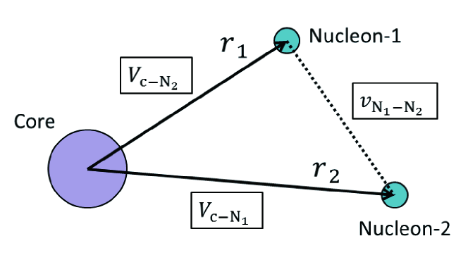
Figure 3.1: A schematic figure for the three-body model defined in the V-coordinates.

3.2 Interactions

In this thesis, we assume that the core-nucleon potential, $V_{\rm c-N}$, is spherical and does not depend on the spin variables. Apart from the Coulomb interaction for a valence proton, we employ the Woods-Saxon potential including the spin-orbit coupling term.

$$V_{\rm c-N,Nucl.}(r) = \left[V_{0}+V_{ls}r_{0}^{2}(\bm{\ell}\cdot\bm{s})\frac{1}{r}\frac{d}{dr}\right]f(r),$$ (3.3)

$$= \left[V_{0}+V_{ls}r_{0}^{2}\left(\frac{j(j+1)-l(l+1)-3/4}{2}\right)\frac{1}{r}\frac{d}{dr}\right]f(r)$$ (3.4)

with

$$f(r)=\frac{1}{1+\exp\left(\frac{r-R_{\rm core}}{a_{\rm core}}\right)},$$ (3.5)

where $R_{\rm core}=r_{0}A_{\rm c}^{1/3}$ is the radius of the core nucleus. In the core-proton case, in addition, the Coulomb potential of a uniform-charged sphere, whose radii and charge are $R_{\rm core}$ and $Z_{\rm c}e$, respectively, is also employed.

$$V_{\rm c-p,Coul.}(r)=\left\{\begin{array}[]{cc}\frac{Z_{\rm c}e^{2}}{4\pi\epsilon_{0}}\frac{1}{r}&(r>R_{\rm core})\\ \frac{Z_{\rm c}e^{2}}{4\pi\epsilon_{0}}\frac{1}{2R_{\rm core}}\left(3-\frac{r^{2}}{R_{\rm core}^{2}}\right)&(r\leq R_{\rm core})\end{array}\right.$$ (3.6)

Thus, the total core-proton potential is given as

$$V_{{\rm c-p},lj}=V_{\rm c-p,Nucl.}(r)+V_{\rm c-p,Coul.}(r).$$ (3.7)

There are four parameters in the core-nucleon potential, namely $V_{0},V_{ls},r_{0}$ and $a_{\rm core}$. We determine the values of these parameters for each system, as we will explain in Chapter 4 and 7.

On the other hand, for the nucleon-nucleon pairing interaction, we adopt the phenomenological “density-dependent contact (DDC)” interaction. It is formulated as

$$v_{\rm N-N,Nucl.}(\bm{r}_{1},\bm{r}_{2})=\delta(\bm{r}_{1}-\bm{r}_{2})\left[v_{0}+\frac{v_{\rho}}{1+\exp\left(\frac{\left|(\bm{r}_{1}+\bm{r}_{2})/2\right|-R_{\rho}}{a_{\rho}}\right)}\right].$$ (3.8)

The first term, $v_{0}\delta(\bm{r}_{1}-\bm{r}_{2})$, indicates the nucleon-nucleon interaction in vacuum, which is approximated to have the zero range. The second term is a phenomenological density-dependent part which is assumed as the Woods-Saxon form. This type of pairing interaction has been employed in several nuclear structural calculations, with a great advantage that it can dramatically reduce the computational cost. These calculations have provided reasonable results [90, 26, 92, 27, 28], despite the simple form of the pairing interaction. Especially, within the three-body model with DDC pairing, the binding energies and the Borromean properties explained in the previous Chapter have been well reproduced for ⁶He and ¹¹Li [26, 92, 27]. In the case with two protons, we also take the Coulomb potential into account.

$$v_{\rm p-p,Coul.}(\bm{r}_{1},\bm{r}_{2})=\frac{e^{2}}{4\pi\epsilon_{0}}\frac{1}{\left|\bm{r}_{1}-\bm{r}_{2}\right|}.$$ (3.9)

For the nuclear part of the pairing interaction, there are four parameters in Eq.(3.8), namely $v_{0},v_{\rho},R_{\rho},a_{\rho}$. The strength of the bare nucleon-nucleon potential, $v_{0}$, can be defined by solving the nucleon-nucleon scattering problem with the bare contact interaction, $v_{0}\delta(\bm{r}_{1}-\bm{r}_{2})$. As well known, this contact interaction must be treated in a truncated space defined with the energy cutoff, $\epsilon_{\rm cut}$, or it loses physical meanings. The strength of the bare interaction, $v_{0}$, can be determined so as to reproduce the empirical scattering length $a_{\rm N-N}$ in the nucleon-nucleon scattering [92]. For a given cutoff $\epsilon_{\rm cut}$, this is formulated as

$$v_{0}=\frac{2\pi^{2}\hbar^{2}}{m}\frac{2a_{\rm N-N}}{\pi-2a_{\rm N-N}k_{\rm cut}},$$ (3.10)

where the relative maximum momentum of two nucleons, $k_{\rm cut}$, is defined as

$$k_{\rm cut}=\sqrt{{m\epsilon_{\rm cut}}/{\hbar^{2}}}.$$ (3.11)

A discussion and derivation of Eq.(3.10) are summarized as Appendix C. The empirical scattering length for a neutron-neutron scattering is $a_{\rm n-n}=-18.5$ fm [147], while that for a proton-proton scattering is $a_{\rm p-p}=-7.81$ fm [148]. The difference between $a_{\rm n-n}$ and $a_{\rm p-p}$ is mainly due to the Coulomb repulsion in a two-proton system. Since we explicitly include the Coulomb interaction in our calculations, we use the neutron-neutron scattering length $a_{\rm n-n}$ to determine the strength of the bare interaction, Eq.(3.10), assuming the charge independence of nuclear force.

Once $v_{0}$ is determined in this way, the remaining parameters in the density-dependent term, $v_{\rho},R_{\rho}$, and $a_{\rho}$ are adjusted to reproduce the three-body binding energy of the considering system. The concrete values of these parameters used in the actual calculations are given in Chapter 4 and 7.

3.3 Single-Particle States

In order to describe an arbitrary wave function, the basis expansion is a popular method. We use this method in our three-body problems. As the first step, we solve the partial core-nucleon wave functions. Because we assumed that the core-nucleon potential, $V_{\rm c-N}$, is spherical and does not depend on the spin variables, the corresponding Schrödinger equation reads

$$h_{i}\phi_{nljm}(\xi_{i})=\epsilon_{nlj}\phi_{nljm}(\xi_{i}).$$ (3.12)

Here we indicate the radial quantum numbers, quantum numbers of orbital angular momenta and of coupled angular momenta as $n,l$ and $j$, respectively. We also need $m$ to indicate the magnetic quantum number. The wave function of the single nucleon can be separated into the radial and the angular parts as

$$\phi_{nljm}(\xi)=R_{nlj}(r)\mathcal{Y}_{ljm}(\bar{\bm{r}},\bm{s})=\frac{U_{nlj}(r)}{r}\mathcal{Y}_{ljm}(\bar{\bm{r}},\bm{s}).$$ (3.13)

where $\bar{\bm{r}}\equiv(\theta,\phi)$. The function $\mathcal{Y}_{ljm}$ indicates the composite angular part of $\bm{j}=\bm{l}+\bm{s}$ coupled to $(j,m)$, that is

$$\hat{\bm{j}}^{2}\mathcal{Y}_{ljm}=j(j+1)\mathcal{Y}_{ljm},~{}~{}~{}~{}~{}~{}\hat{j_{z}}\mathcal{Y}_{ljm}=m\mathcal{Y}_{ljm}.$$ (3.14)

Using the Clebsch-Gordan coefficients, its explicit form is given as

$$\mathcal{Y}_{ljm}(\bar{\bm{r}},\bm{s}) \equiv \Braket{\bar{\bm{r}},\bm{s}\mid(l\oplus 1/2)\phantom{0}j,m}$$ (3.15)

$$= \sum_{h}\sum_{v}\mathcal{C}^{j,m}_{l,h;1/2,v}Y_{lh}(\bar{\bm{r}})\chi_{v}(\bm{s}),$$ (3.16)

where $Y_{lh}$ and $\chi_{v}$ satisfy

$$\hat{\bm{l}}^{2}Y_{lh}(\bar{\bm{r}})=l(l+1)Y_{lh}(\bar{\bm{r}}), ~{}~{}\hat{l}_{z}Y_{lh}(\bar{\bm{r}})=hY_{lh}(\bar{\bm{r}}),$$ (3.17)

$$\hat{\bm{s}}^{2}\chi_{v}(\bm{s})=\frac{3}{4}\chi_{v}(\bm{s}), ~{}~{}\hat{s}_{z}\chi_{v}(\bm{s})=v\chi_{v}(\bm{s}),$$ (3.18)

with $h=-l\sim l$ and $v=\pm 1/2$. Then Eq.(3.12) can be reduced to the equation only for the radial part $R_{nlj}$. That is

$$\left[-\frac{\hbar^{2}}{2\mu}\left(\frac{1}{r}\frac{d^{2}}{dr^{2}}r-\frac{l(l+1)}{r^{2}}\right)+V_{{\rm c-N},lj}(r)\right]R_{nlj}(r)=\epsilon_{nlj}R_{nlj}(r),$$ (3.19)

or equivalently for $U_{nlj}(r)=rR_{nlj}$,

$$\left[\frac{d^{2}}{dr^{2}}-\frac{l(l+1)}{r^{2}}-\frac{2\mu}{\hbar^{2}}\left(V_{{\rm c-N},lj}(r)-\epsilon_{nlj}\right)\right]U_{nlj}(r)=0.$$ (3.20)

In this thesis, we solve the radial part $U_{nlj}$ numerically within a discrete variable-domain. Assuming a radial box with its size $R_{\rm box}$, sampling points are distributed in the interval $0\sim R_{\rm box}$ where the distance between two consecutive points is $dr=r_{n-1}-r_{n}$. For the continuum s.p. states with $\epsilon_{nlj}>V_{{\rm c-N},lj}(r\to\infty)\equiv 0$, we assume the boundary condition with a vanishing wave function at $r=R_{\rm box}$. That is

$$U_{nlj}(r=R_{\rm box})=0.$$ (3.21)

Because of this boundary condition, the continuum energy spectrum is discretized. Either for the bound and the discretized continuum s.p. states, their radial wave functions can be calculated numerically. The numerical method we employ in this thesis is “Numerov method”, which was developed by B. V. Numerov [149]. A detailed introduction of this method is separately summarized as Appendix A.

3.4 Uncorrelated Basis for Two Nucleons

Using s.p. wave functions $\{\phi_{nljm}\}$ obtained in the previous section, the “uncorrelated basis” for two-nucleon states can be constructed. If two nucleons are coupled to the spin $(J,M)$, the uncorrelated states are formulated as

$$\Psi^{(J,M)}_{ab}(\xi_{1},\xi_{2}) = \Psi^{(J,M)}_{(nlj)_{a}(nlj)_{b}}(\xi_{1},\xi_{2})\equiv\left[\phi_{(nlj)_{a}}(\xi_{1})\otimes\phi_{(nlj)_{b}}(\xi_{2})\right]^{(J,M)}$$ (3.22)

$$= R_{(nlj)_{a}}(r_{1})R_{(nlj)_{b}}(r_{2})\cdot W^{(J,M)}_{ab}(\bar{\bm{r}}_{1}\bm{s}_{1},\bar{\bm{r}}_{2}\bm{s}_{2}),$$ (3.23)

where we define the shortened subscripts $(nlj)_{a}\equiv(n_{a},l_{a},j_{a})$. The coupled angular part, $W^{(J,M)}_{ab}$, is defined as

$$W^{(J,M)}_{ab}(\bar{\bm{r}}_{1}\bm{s}_{1},\bar{\bm{r}}_{2}\bm{s}_{2})\equiv\Braket{\bar{\bm{r}}_{1}\bm{s}_{1},\bar{\bm{r}}_{2}\bm{s}_{2}\mid(j_{a}\oplus j_{b})~{}J,M}$$ (3.24)

$$~{}~{}~{}~{}=\sum_{m_{a},m_{b}}\mathcal{C}^{J,M}_{j_{a},m_{a};j_{b},m_{b}}\mathcal{Y}_{(ljm)_{a}}(\bar{\bm{r}}_{1},\bm{s}_{1})\mathcal{Y}_{(ljm)_{b}}(\bar{\bm{r}}_{2},\bm{s}_{2}).$$ (3.25)

This function means that the first and the second valence nucleons are in the core-nucleon orbits labeled by $(n_{a},l_{a},j_{a})$ and $(n_{b},l_{b},j_{b})$, respectively. In actual calculations, we also add another constraint of the total parity, by including only those configurations with the same value of $\pi=(-)^{l_{a}+l_{b}}$ in defining basis. For two nucleons of the same kind, we have to take the anti-symmetrization into account. That is

$$\tilde{\Psi}^{(J,M)}_{ab}(\xi_{1},\xi_{2})\equiv A_{ab}\left[\Psi^{(J,M)}_{ab}(\xi_{1},\xi_{2})-\Psi^{(J,M)}_{ab}(\xi_{2},\xi_{1})\right],$$ (3.26)

where $A_{ab}$ is the normalization factor. This is given as

$$A_{ab}=\left\{\begin{array}[]{cc}1/2&(n_{a}=n_{b}\cap l_{a}=l_{b}\cap j_{a}=j_{b})\\ 1/\sqrt{2}&({\rm otherwise})\end{array}\right.$$ (3.27)

If we write it explicitly, Eq.(3.26) is given as

$$\tilde{\Psi}^{(J,M)}_{ab}(\xi_{1},\xi_{2}) = A_{ab}\left[R_{(nlj)_{a}}(r_{1})R_{(nlj)_{b}}(r_{2})\cdot W^{(J,M)}_{ab}(\bar{\bm{r}}_{1}\bm{s}_{1},\bar{\bm{r}}_{2}\bm{s}_{2})\right.$$ (3.28)

$$\;\;-\left.R_{(nlj)_{a}}(r_{2})R_{(nlj)_{b}}(r_{1})\cdot W^{(J,M)}_{ab}(\bar{\bm{r}}_{2}\bm{s}_{2},\bar{\bm{r}}_{1}\bm{s}_{1})\right].$$

Using the formula of the Clebsch-Gordan coefficients;

$$\mathcal{C}^{J,M}_{j_{a},m_{a};j_{b},m_{b}}=(-)^{j_{a}+j_{b}-J}\mathcal{C}^{J,M}_{j_{b},m_{b};j_{a},m_{a}},$$ (3.29)

the coupled angular part of the second term in Eq.(3.28) can be transformed to

$$W^{(J,M)}_{ab}(\bar{\bm{r}}_{2}\bm{s}_{2},\bar{\bm{r}}_{1}\bm{s}_{1})$$

$$~{}~{}~{}~{}=\sum_{m_{a},m_{b}}\mathcal{C}^{J,M}_{j_{a},m_{a};j_{b},m_{b}}\mathcal{Y}_{(ljm)_{a}}(\bar{\bm{r}}_{2},\bm{s}_{2})\mathcal{Y}_{(ljm)_{b}}(\bar{\bm{r}}_{1},\bm{s}_{1})$$

$$~{}~{}~{}~{}=(-)^{j_{a}+j_{b}-J}\sum_{m_{a},m_{b}}\mathcal{C}^{J,M}_{j_{b},m_{b};j_{a},m_{a}}\mathcal{Y}_{(ljm)_{a}}(\bar{\bm{r}}_{2},\bm{s}_{2})\mathcal{Y}_{(ljm)_{b}}(\bar{\bm{r}}_{1},\bm{s}_{1})$$

$$~{}~{}~{}~{}=(-)^{j_{a}+j_{b}-J}W^{(J,M)}_{ba}(\bar{\bm{r}}_{1}\bm{s}_{1},\bar{\bm{r}}_{2}\bm{s}_{2}).$$ (3.30)

Thus we obtain another formula for $\tilde{\Psi}^{(J,M)}_{ab}$.

$$\tilde{\Psi}^{(J,M)}_{ab}(\xi_{1},\xi_{2})=A_{ab}\left[\Psi^{(J,M)}_{nlj(a),nlj(b)}(\xi_{1},\xi_{2})-B_{ab}\Psi^{(J,M)}_{nlj(b),nlj(a)}(\xi_{1},\xi_{2})\right]$$ (3.31)

with $B_{ab}\equiv(-)^{j_{a}+j_{b}-J}$. Notice that $\tilde{\Psi}^{(J,M)}_{ab}$ is an eigenstate of the uncorrelated Hamiltonian, $h_{1}+h_{2}$. Its eigen-equation reads

$$(h_{1}+h_{2})\tilde{\Psi}^{(J,M)}_{ab}=(\epsilon_{a}+\epsilon_{b})\tilde{\Psi}^{(J,M)}_{ab},$$ (3.32)

where $\epsilon_{a}$ and $\epsilon_{b}$ are the eigen-energies of the first and the second orbits, respectively.

We can now expand an arbitrary two-nucleon state with $(J,M)$ on the uncorrelated basis. That is,

$$\Phi^{(J,M)}(\xi_{1},\xi_{2})=\sum_{a\leq b}\alpha_{ab}\tilde{\Psi}^{(J,M)}_{ab}(\xi_{1},\xi_{2}).$$ (3.33)

where our model-space is truncated by the cutoff energy for the uncorrelated basis, defined as $E_{\rm cut}=\epsilon_{\rm cut}(A_{\rm c}+1)/A_{\rm c}$ [92]. In practice, we have to introduce also the cutoff angular momentum, $l_{\rm cut}$, in addition to $E_{\rm cut}$. Notice that Matsuo et.al. have shown that the spatial localization cannot be reproduced theoretically unless one includes a sufficient number of angular momenta. Referring to their results, we would have to employ the model-space with, at least, up to $l_{\rm max}=5$ in order to take the dinucleon correlations into account.

In the following, for simplicity, we omit the subscripts $(J,M)$ unless it is needed. For the eigenstates of $H_{\rm 3b}$, namely $H_{\rm 3b}\ket{\Phi_{N}}=E_{N}\ket{\Phi_{N}}$, the expansion coefficients $\{\alpha_{ab}\}$ can be obtained by diagonalizing the Hamiltonian matrix. In the next section, we detail how to calculate these matrix elements.

3.5 Matrix Elements with Uncorrelated Basis

First, for the uncorrelated Hamiltonian, $h_{1}+h_{2}$, the matrix elements are trivially given as

$$\Braket{\tilde{\Psi}_{cd}\mid(h_{1}+h_{2})\mid\tilde{\Psi}_{ab}}=(\epsilon_{a}+\epsilon_{b})\delta_{cd,ab},$$ (3.34)

where $\epsilon_{a}\equiv\epsilon_{n_{a}l_{a}j_{a}}$. For the other parts of the Hamiltonian, we need much complicated calculations in general. A matrix element (ME) of an arbitrary operator, $\hat{\mathcal{O}}$, is decomposed into four terms,

$$\Braket{\tilde{\Psi}_{cd}\mid\hat{\mathcal{O}}\mid\tilde{\Psi}_{ab}} = A_{cd}A_{ab}\left[\Braket{\Psi_{cd}\mid\hat{\mathcal{O}}\mid\Psi_{ab}}+B_{cd}B_{ab}\Braket{\Psi_{dc}\mid\hat{\mathcal{O}}\mid\Psi_{ba}}\right.$$ (3.35)

$$\left.-B_{ab}\Braket{\Psi_{cd}\mid\hat{\mathcal{O}}\mid\Psi_{ba}}-B_{cd}\Braket{\Psi_{dc}\mid\hat{\mathcal{O}}\mid\Psi_{ab}}\right]$$

where we have applied Eq.(3.31). In the following subsections, we explain how to calculate MEs of several important operators.

3.5.1 Single Particle Operators

This kind of operators is characterized as $\hat{\mathcal{O}}=O(\xi_{1})+O(\xi_{2})$. These include the core-nucleon interaction $V_{\rm c-N}(\xi_{i})$, the s.p. kinetic energy $\bm{p}^{2}_{i}/2\mu=h_{i}-V_{\rm c-N}(\xi_{i})$, the radial distance $\left|\bm{r}_{i}\right|^{2}$, and so on. For the operator $\hat{\mathcal{O}}(1)=O(\xi_{1})$ which acts only on the first particle, the first term in Eq.(3.35) has the form of

$$\Braket{\Psi_{cd}\mid\hat{\mathcal{O}}(1)\mid\Psi_{ab}} = \int d\xi_{1}\int d\xi_{2}\Psi_{cd}^{*}(\xi_{1},\xi_{2})O(\xi_{1})\Psi_{ab}(\xi_{1},\xi_{2})$$ (3.37)

$$= \delta_{d,b}\sum_{m_{c},m_{a}}\mathcal{C}^{J,M*}_{j_{d},M-m_{c};j_{c},m_{c}}\mathcal{C}^{J,M}_{j_{b},M-m_{a};j_{a},m_{a}}$$

$$\phantom{000}\times\int d\xi_{1}\phi^{*}_{(nljm)_{c}}(\xi_{1})O(\xi_{1})\phi_{(nljm)_{a}}(\xi_{1}),$$

which vanishes if $n_{b}\neq n_{d}\cup l_{b}\neq l_{d}\cup j_{b}\neq j_{d}$. Thus, the only quantity we have to calculate is the integration in the last sentence. The other terms in Eq.(3.35) can be calculated similarly. Defining the following symbol;

$$O_{ca}^{(1)} \equiv \sum_{m_{c},m_{a}}\mathcal{C}^{J,M*}_{j_{d},M-m_{c};j_{c},m_{c}}\mathcal{C}^{J,M}_{j_{b},M-m_{a};j_{a},m_{a}}$$ (3.38)

$$\phantom{000}\times\int d\xi_{1}\phi^{*}_{(nljm)_{c}}(\xi_{1})O(\xi_{1})\phi_{(nljm)_{a}}(\xi_{1}),$$

we can represent the matrix element of $\hat{\mathcal{O}}(1)=O(\xi_{1})$ after the anti-symmetrization as follows.

$$\Braket{\tilde{\Psi}_{cd}\mid\hat{\mathcal{O}}(1)\mid\tilde{\Psi}_{ab}} = A_{cd}A_{ab}\left[\delta_{db}O_{ca}^{(1)}+B_{cd}B_{ab}\delta_{ca}O_{bd}^{(1)}\right.$$ (3.39)

$$\left.-B_{ab}\delta_{cb}O_{da}^{(1)}-B_{cd}\delta_{da}O_{cb}^{(1)}\right].$$

We also derive the similar formula for the summation of $\hat{\mathcal{O}}(1)$ and $\hat{\mathcal{O}}(2)$. The result reads

$$\Braket{\tilde{\Psi}_{cd}\mid\hat{\mathcal{O}}(1)+\hat{\mathcal{O}}(2)\mid\tilde{\Psi}_{ab}}$$

$$\phantom{000}=A_{cd}A_{ab}\left[\delta_{db}(O_{ca}^{(1)}+B_{cd}B_{ab}O_{ca}^{(2)})+\delta_{ca}(B_{cd}B_{ab}O_{db}^{(1)}+O_{db}^{(2)})\right.$$

$$\phantom{000000000000}\left.-\delta_{cb}(B_{cd}O_{da}^{(1)}+B_{ab}O_{da}^{(2)})-\delta_{da}(B_{ab}O_{cb}^{(1)}+B_{cd}O_{cb}^{(2)})\right].$$ (3.40)

We will use this formula to calculate, e.g. those of $h_{1}+h_{2}$ or $V_{\rm c-N}(\xi_{1})+V_{\rm c-N}(\xi_{2})$.

If the operator is spherical; $O(\xi_{1})=O(r_{1})$, Eq.(3.38) can be reduced as the integration only for the radial distance.

$$O_{ca}^{(1),spherical} = \delta_{j_{c}j_{a}}\delta_{l_{c}l_{a}}\int dr_{1}r_{1}^{2}R_{(nlj)_{c}}(r_{1})O(r_{1})R_{(nlj)_{a}}(r_{1}),$$ (3.41)

$$= \delta_{j_{c}j_{a}}\delta_{l_{c}l_{a}}\int dr_{1}U_{(nlj)_{c}}(r_{1})O(r_{1})U_{(nlj)_{a}}(r_{1}),$$

where the product of coupled angular parts is given as $\delta_{j_{c},j_{a}}\delta_{l_{c},l_{a}}$.

3.5.2 Two-Particle Operators

The Operators in this category are given as $\hat{\mathcal{O}}=O(\xi_{1},\xi_{2})$. These include, for instance, the pairing interaction, $v_{\rm N-N}$, the recoil term, $\bm{p}_{1}\cdot\bm{p}_{2}/A_{\rm c}m$, and the opening angle between two nucleons, $\cos\theta_{12}$. In order to calculate Eq.(3.35), it is often necessary to know the following quantity.

$$\Braket{\mathcal{Y}_{(ljm)_{c}}\mid Y_{lh}\mid\mathcal{Y}_{(ljm)_{a}}}=\int d\bar{\bm{r}}\int d\bm{s}\mathcal{Y}^{*}_{(ljm)_{c}}(\bar{\bm{r}},\bm{s})Y_{lh}(\bar{\bm{r}})\mathcal{Y}_{(ljm)_{a}}(\bar{\bm{r}},\bm{s})$$ (3.42)

For this purpose, one can use the Wigner-Eckart theorem found in, e.g. the textbook by Edmonds [150],

$$\Braket{\mathcal{Y}_{(ljm)_{c}}\mid Y_{lh}\mid\mathcal{Y}_{(ljm)_{a}}}$$

$$~{}~{}~{}=(-)^{j_{a}-m_{a}-2h}\frac{\mathcal{C}^{l,h}_{j_{c},m_{c};j_{a},m_{a}}}{\sqrt{2l+1}}\Braket{j_{c}(l_{c},1/2)}{Y_{l}}{j_{a}(l_{a},1/2)},$$ (3.43)

where the reduced matrix element is written with the $6j$-symbols as

$$\Braket{j_{c}(l_{c},1/2)}{Y_{l}}{j_{a}(l_{a},1/2)} = (-)^{l_{c}+l_{a}+j_{a}+l}\sqrt{(2j_{c}+1)(2j_{a}+1)}$$ (3.46)

$$\times\left\{\begin{array}[]{ccc}l_{c}&j_{c}&1/2\\ j_{a}&1/2&l\end{array}\right\}\Braket{l_{c}}{Y_{l}}{l_{a}},$$

$$\Braket{l_{c}}{Y_{l}}{l_{a}} = (-)^{l_{c}+l}\frac{\sqrt{(2l_{c}+1)(2l_{a}+1)}}{4\pi}\mathcal{C}^{l,0}_{l_{c},0;l_{a};0}.$$

When the operator is scalar and does not include spin variables, it can be generally represented by the multi-pole expansion. Namely,

$$O(\bm{r}_{1},\bm{r}_{2})=\sum_{l=0}^{\infty}O_{l}(r_{1},r_{2})\sum_{h=-l}^{l}Y_{l,h}(\bar{\bm{r}}_{1})\cdot(-)^{h}Y_{l,-h}(\bar{\bm{r}}_{2}).$$ (3.47)

Then, we can formulate each component in Eq.(3.35). For the $l$-th term in Eq.(3.47), the radial part becomes

$$rad.part_{(l)}\left[\Braket{\Psi_{cd}\mid\hat{\mathcal{O}}(1,2)\mid\Psi_{ab}}\right]$$

$$~{}=\iint dr_{1}dr_{2}R^{*}_{(nlj)_{c}}(r_{1})R^{*}_{(nlj)_{d}}(r_{2})O_{l}(r_{1},r_{2})R_{(nlj)_{a}}(r_{1})R_{(nlj)_{b}}(r_{2}),$$ (3.48)

whereas the angular part is given as

$$ang.part_{(l)}\left[\Braket{\Psi_{cd}\mid\hat{\mathcal{O}}(1,2)\mid\Psi_{ab}}\right]$$

$$~{}~{}~{}=\left<(j_{c}\oplus j_{d})J,M\mid\sum_{h}Y_{lh}(1)(-)^{h}Y_{l,-h}(2)\mid(j_{a}\oplus j_{b})J,M\right>$$

$$~{}~{}~{}=\sum_{all~{}m}\mathcal{C}^{*J,M}_{j_{c},m_{c};j_{d},m_{d}}\mathcal{C}^{J,M}_{j_{a},m_{a};j_{b},m_{b}}$$

$$~{}~{}~{}~{}~{}~{}~{}\sum_{h}\Braket{\mathcal{Y}_{(ljm)_{c}}\mid Y_{l,h}\mid\mathcal{Y}_{(ljm)_{a}}}(-)^{h}\Braket{\mathcal{Y}_{(ljm)_{d}}\mid Y_{l,-h}\mid\mathcal{Y}_{(ljm)_{b}}}.$$ (3.49)

By performing a few calculations for the angular momenta, Eq.(3.49) can be simplified as

$$ang.part_{(l)}\left[\Braket{\Psi_{cd}\mid\hat{\mathcal{O}}(1,2)\mid\Psi_{ab}}\right]$$

$$~{}~{}=(-)^{j_{a}+j_{d}-J}\left\{\begin{array}[]{ccc}j_{a}&l&j_{c}\\ j_{d}&J&j_{b}\end{array}\right\}$$ (3.52)

$$\phantom{00000}\times\Braket{j_{c}(l_{c},1/2)}{Y_{l}}{j_{a}(l_{a},1/2)}\cdot\Braket{j_{d}(l_{d},1/2)}{Y_{l}}{j_{b}(l_{b},1/2)},$$ (3.53)

where the summations over the magnetic quantum numbers do not appear [150]. Consequently, we can write down the general formula for the ME of a two-particle operator as

$$\Braket{\Psi_{cd}\mid\hat{\mathcal{O}}(1,2)\mid\Psi_{ab}}$$

$$~{}~{}=\sum_{l}\iint dr_{1}dr_{2}R^{*}_{(nlj)_{c}}(r_{1})R^{*}_{(nlj)_{d}}(r_{2})O_{l}(r_{1},r_{2})R_{(nlj)_{a}}(r_{1})R_{(nlj)_{b}}(r_{2})$$

$$\phantom{00000}\times(-)^{j_{a}+j_{d}-J}\left\{\begin{array}[]{ccc}j_{a}&l&j_{c}\\ j_{d}&J&j_{b}\end{array}\right\}$$ (3.56)

$$\phantom{0000000}\Braket{j_{c}(l_{c},1/2)}{Y_{l}}{j_{a}(l_{a},1/2)}\cdot\Braket{j_{d}(l_{d},1/2)}{Y_{l}}{j_{b}(l_{b},1/2)}.$$ (3.57)

We mention that the orbital angular momenta, $l$, must be truncated in actual calculations. Thus, the summation over $l$ is also truncated as $\sum_{l=0}^{\infty}\rightarrow\sum_{l=0}^{l_{\rm max}}$.

We also mention how to derive the $O_{l}(r_{1},r_{2})$. For the pairing interaction, the two-particle operator depends only on the relative distance,

$$r_{12}=\left|\bm{r}_{1}-\bm{r}_{2}\right|=\sqrt{r_{1}^{2}+r_{2}^{2}-2r_{1}r_{2}\cos\theta_{12}}.$$ (3.58)

The multi-pole expansion for an arbitrary function of $r_{12}$ satisfies

$$f(r_{12}) = \sum_{l=0}^{l_{\rm max}}(2l+1)g_{l}(r_{1},r_{2})P_{l}(\cos\theta_{12})$$ (3.59)

$$= \sum_{l=0}^{l_{\rm max}}g_{l}(r_{1},r_{2})4\pi\sum_{h=-l}^{l}Y_{l,h}(\bar{\bm{r}}_{1})(-)^{h}Y_{l,-h}(\bar{\bm{r}}_{2}),$$ (3.60)

with

$$g_{l}(r_{1},r_{2})=\frac{1}{2}\int_{0}^{\pi}f(r_{12})P_{l}(\cos\theta_{12})\sin\theta_{12}d\theta_{12},$$ (3.61)

where $P_{l}$ is the Legendre polynomial. We list below concrete forms of the functions used for the pairing interaction.

1. a delta function;

   $$f(r_{12})=\delta(\left|\bm{r}_{1}-\bm{r}_{2}\right|)=\frac{\delta(r_{1}-r_{2})}{r_{1}r_{2}}\sum_{l}\sum_{h=-l}^{l}Y_{l,h}(\bar{\bm{r}}_{1})(-)^{h}Y_{l,-h}(\bar{\bm{r}}_{2}).$$ (3.62)

2. an inverse function;

   $$f(r_{12})=\frac{1}{\left|\bm{r}_{1}-\bm{r}_{2}\right|}=\sum_{l}\frac{r_{<}^{l}}{r_{>}^{l+1}}\frac{4\pi}{2l+1}\sum_{h=-l}^{l}Y_{l,h}(\bar{\bm{r}}_{1})(-)^{h}Y_{l,-h}(\bar{\bm{r}}_{2}),$$ (3.63)

   where $r_{>}$ ($r_{<}$) indicates the larger (smaller) one between $r_{1}$ and $r_{2}$.

On the other hand, for the recoil term; $\bm{p}_{1}\cdot\bm{p}_{2}/A_{\rm c}m$, we first use the formula of the spatial differentiation, that is

$$\frac{1}{2}\left[\nabla^{2},\bm{r}\right]=\nabla\Longleftrightarrow\nabla=\bar{\bm{r}}\left(\frac{d}{dr}+\frac{1}{r}\right)-\frac{1}{2r}\left[\hat{\bm{l}}^{2},\bar{\bm{r}}\right].$$ (3.64)

Thus, for the product $\nabla_{1}\cdot\nabla_{2}$, its ME before the anti-symmetrization takes the form of

$$\Braket{\Psi_{cd}}{\nabla_{1}\cdot\nabla_{2}}{\Psi_{ab}}$$

$$~{}~{}~{}=\left<R_{c}R_{d}\mid\left\{(\frac{d}{dr_{1}}+\frac{1}{r_{1}})-\frac{1}{2r_{1}}(l_{c}(l_{c}+1)-l_{a}(l_{a}+1))\right\}\right.$$

$$~{}~{}~{}~{}~{}~{}~{}~{}\left.\left\{(\frac{d}{dr_{2}}+\frac{1}{r_{2}})-\frac{1}{2r_{2}}(l_{d}(l_{d}+1)-l_{b}(l_{b}+1))\right\}\mid R_{a}R_{b}\right>$$

$$~{}~{}~{}~{}~{}\times\Braket{W_{cd}\mid\bar{\bm{r}}_{1}\cdot\bar{\bm{r}}_{2}\mid W_{ab}},$$ (3.65)

where the radial part can be calculated with the first derivatives. In the angular part, we expand the function, $\bar{\bm{r}}_{1}\cdot\bar{\bm{r}}_{2}$, as follows.

$$\bar{\bm{r}}_{1}\cdot\bar{\bm{r}}_{2}=\cos\theta_{12}=P_{l=1}(\cos\theta_{12})=\frac{4\pi}{3}\sum_{h=-1}^{1}Y_{1,h}(\bar{\bm{r}}_{1})(-)^{h}Y_{1,-h}(\bar{\bm{r}}_{2}).$$ (3.66)

Consequently, the MEs of this operator can be calculated by means of the dipole expansion.

$$\Braket{W_{cd}\mid\bar{\bm{r}}_{1}\cdot\bar{\bm{r}}_{2}\mid W_{ab}}$$

$$~{}~{}=\frac{4\pi}{3}(-)^{j_{a}+j_{d}-J}\left\{\begin{array}[]{ccc}j_{a}&1&j_{c}\\ j_{d}&J&j_{b}\end{array}\right\}$$ (3.69)

$$\phantom{00000}\times\Braket{j_{c}(l_{c},1/2)}{Y_{1}}{j_{a}(l_{a},1/2)}\cdot\Braket{j_{d}(l_{d},1/2)}{Y_{1}}{j_{b}(l_{b},1/2)}.$$ (3.70)

Obviously, the recoil term mixes the uncorrelated basis which satisfy $\left|l_{c}-l_{a}\right|=1$. If we limit the model space with $(-)^{l_{a}}=odd$ or $even$ only, the recoil term does not contribute.

3.6 Density Distribution

We also derive the formulas for the density distributions of two nucleons. With our uncorrelated basis, the two-nucleon state can be expanded as Eq.(3.33). Its density distribution is obviously given by

$$\rho(\xi_{1},\xi_{2}) = \left|\Phi(\xi_{1},\xi_{2})\right|^{2}=\sum_{34}\sum_{12}\alpha_{34}^{*}\alpha_{12}\tilde{\Psi}_{34}^{*}\cdot\tilde{\Psi}_{12}(\xi_{1},\xi_{2})$$ (3.72)

$$= \sum_{34}\sum_{12}\alpha_{34}^{*}\alpha_{12}A_{34}A_{12}$$

$$\times\left[\pi_{34,12}(\xi_{1},\xi_{2})+B_{34}B_{12}\pi_{43,21}-B_{34}\pi_{43,12}-B_{12}\pi_{34,21}\right],$$

with $B_{ab}\equiv(-)^{j_{a}+j_{b}-J}$. Each component $\pi_{cd,ab}(\xi_{1},\xi_{2})$ can be written as

$$\pi_{34,12}(\xi_{1},\xi_{2}) \equiv \Psi_{34}^{*}\cdot\Psi_{12}(\xi_{1},\xi_{2})$$ (3.74)

$$= \left[\sum_{m_{3}}\mathcal{C}^{J,M}_{j_{3},m_{3};j_{4},M-m_{3}}\phi_{(nljm)_{3}}(\xi_{1})\phi_{(nljm)_{4}}(\xi_{2})\right]^{*}\times$$

$$\left[\sum_{m_{1}}\mathcal{C}^{J,M}_{j_{1},m_{1};j_{2},M-m_{1}}\phi_{(nljm)_{1}}(\xi_{1})\phi_{(nljm)_{2}}(\xi_{2})\right]$$

$$= R^{*}_{(nlj)_{3}}(r_{1})R^{*}_{(nlj)_{4}}(r_{2})\cdot R_{(nlj)_{1}}(r_{1})R_{(nlj)_{2}}(r_{2})$$

$$\times~{}W_{34}^{*(J,M)}(\bar{\bm{r}}_{1}\bm{s}_{1},\bar{\bm{r}}_{2}\bm{s}_{2})\cdot W_{12}^{(J,M)}(\bar{\bm{r}}_{1}\bm{s}_{1},\bar{\bm{r}}_{2}\bm{s}_{2}).$$

where we used the Eqs(3.23) and (3.24).

3.7 Spin-Orbit Decomposition

It will be also helpful to formulate the decomposition of two-nucleon states into those of the spin-singlet and triplet configurations. For this purpose, at first, we have to discuss some mathematics of angular momenta. In Eq.(3.24), to fix the final angular momentum, $(J,M)$, we first couple $\bm{l}_{a}$ and $\bm{s}_{1}$ to $\bm{j}_{a}$, and then couple $\bm{j}_{a}$ and $\bm{j}_{b}$ to $\bm{J}$. That is,

$$\left.\begin{array}[]{c}\bm{l}_{a}\oplus\bm{s}_{1}=\bm{j}_{a}\\ \bm{l}_{b}\oplus\bm{s}_{2}=\bm{j}_{b}\end{array}\right\}\longrightarrow\bm{j}_{a}\oplus\bm{j}_{b}=\bm{J},$$ (3.75)

where $s_{i}=\left|\bm{s}_{i}\right|=1/2$. Within this coupling scheme, we got the coupled angular part, $W_{ab}^{(J,M)}=W_{l_{a}l_{b}j_{a}j_{b}}^{(J,M)}(\bar{\bm{r}}_{1}\bm{s}_{1},\bar{\bm{r}}_{2}\bm{s}_{2})$. On the other hand, another coupling scheme can be considered as

$$\left.\begin{array}[]{c}\bm{l}_{a}\oplus\bm{l}_{b}=\bm{L}\\ \bm{s}_{1}\oplus\bm{s}_{2}=\bm{S}\end{array}\right\}\longrightarrow\bm{L}\oplus\bm{S}=\bm{J}.$$ (3.76)

Those two coupling schemes can be related to each other by the unitary transformation. Namely, we can write down

$$W_{l_{a}l_{b}j_{a}j_{b}}^{(J,M)}(\bar{\bm{r}}_{1}\bm{s}_{1},\bar{\bm{r}}_{2}\bm{s}_{2})$$

$$~{}~{}~{}~{}~{}~{}~{}=\sum_{L=|l_{a}-l_{b}|}^{l_{a}+l_{b}}\sum_{S=0,1}D_{J}(j_{a}j_{b};l_{a}l_{b}s_{1}s_{2};LS)\cdot\Xi_{l_{a}l_{b}LS}^{(J,M)}(\bar{\bm{r}}_{1}\bm{s}_{1},\bar{\bm{r}}_{2}\bm{s}_{2}),$$ (3.77)

with the $LS$-coupled angular part;

$$\Xi_{l_{a}l_{b}LS}^{(J,M)}(\bar{\bm{r}}_{1}\bm{s}_{1},\bar{\bm{r}}_{2}\bm{s}_{2})=\sum_{M_{S}=\pm 1}\mathcal{C}^{J,M}_{L,M-V;S,M_{S}}$$

$$~{}~{}~{}~{}~{}~{}~{}~{}~{}~{}~{}~{}~{}\times\left[Y_{l_{a}}(\bar{\bm{r}}_{1})\otimes Y_{l_{b}}(\bar{\bm{r}}_{2})\right]^{(L,M-V)}\left[\chi(\bm{s}_{1})\otimes\chi(\bm{s}_{2})\right]^{(S,V)},$$ (3.78)

and the expansion coefficients including the $9j$-symbol;

$$D_{J}(j_{a}j_{b};l_{a}l_{b}s_{1}s_{2};LS)$$

$$~{}~{}~{}~{}~{}~{}~{}\equiv\sqrt{(2L+1)(2S+1)(2j_{a}+1)(2j_{b}+1)}\left\{\begin{array}[]{ccc}l_{a}&l_{b}&L\\ s_{1}&s_{2}&S\\ j_{a}&j_{b}&J\end{array}\right\}.$$ (3.82)

Using these formulas, the anti-symmetrized uncorrelated basis can be decomposed into the spin-singlet and triplet configurations as follows.

$$\tilde{\Psi}_{ab}(\xi_{1},\xi_{2}) = \tilde{\Psi}_{ab,S=0}(\xi_{1},\xi_{2})+\tilde{\Psi}_{ab,S=1}(\xi_{1},\xi_{2}),$$ (3.83)

$$\tilde{\Psi}_{ab,S}(\xi_{1},\xi_{2}) = A_{ab}\left[\Psi_{ab,S}(\xi_{1},\xi_{2})-B_{ab}\Psi_{ba,S}(\xi_{1},\xi_{2})\right],$$ (3.84)

with

$$\Psi_{ab,S}(\xi_{1},\xi_{2})=R_{(nlj)_{a}}(r_{1})R_{(nlj)_{b}}(r_{2})$$

$$~{}~{}~{}~{}~{}~{}\times\sum_{L=|l_{a}-l_{n}|}^{l_{a}+l_{b}}D_{J}(j_{a}j_{b};l_{a}l_{b}s_{1}s_{2};LS)\cdot\Xi_{l_{a}l_{b}LS}^{(J,M)}(\bar{\bm{r}}_{1}\bm{s}_{1},\bar{\bm{r}}_{2}\bm{s}_{2}).$$ (3.85)

Notice that the normalization of each basis function reads

$$1 = \int d\xi_{1}\int d\xi_{2}\left|\tilde{\Psi}_{ab}(\xi_{1},\xi_{2})\right|^{2}$$ (3.87)

$$= \int d\bm{r}_{1}\int d\bm{r}_{2}\left\{\left|\tilde{\Psi}_{ab,S=0}(\bm{r}_{1},\bm{r}_{2})\right|^{2}+\left|\tilde{\Psi}_{ab,S=1}(\bm{r}_{1},\bm{r}_{2})\right|^{2}\right\}$$

$$= \left|A_{ab}\right|^{2}\sum_{S}\sum_{L}\left\{\left|D_{J}(j_{a}j_{b};l_{a}l_{b}s_{1}s_{2};LS)\right|^{2}+\left|D_{J}(j_{a}j_{b};l_{a}l_{b}s_{1}s_{2};LS)\right|^{2}\right.$$

$$-B_{ab}D^{*}_{J}(j_{b}j_{a};l_{b}l_{a}s_{2}s_{1};LS)D_{J}(j_{a}j_{b};l_{a}l_{b}s_{1}s_{2};LS)\delta_{n_{b},n_{a}}$$

$$\left.-B_{ab}D^{*}_{J}(j_{a}j_{b};l_{a}l_{b}s_{1}s_{2};LS)D_{J}(j_{b}j_{a};l_{b}l_{a}s_{2}s_{1};LS)\delta_{n_{b},n_{a}}\right\},$$

where the radial integrations in the cross terms become $\delta_{n_{b},n_{a}}$. We also introduce a similar decomposition for the density distribution. Namely, Eq.(3.74) can be decomposed as

$$\pi_{34,12}(\xi_{1},\xi_{2}) \equiv \Psi_{34}^{*}\cdot\Psi_{12}(\xi_{1},\xi_{2})$$ (3.88)

$$= R^{*}_{(nlj)_{3}}(r_{1})R^{*}_{(nlj)_{4}}(r_{2})\cdot R_{(nlj)_{1}}(r_{1})R_{(nlj)_{2}}(r_{2})$$

$$\times\sum_{L^{\prime},S^{\prime}}\left[D_{J}(j_{3}j_{4};l_{3}l_{4}s_{3}s_{4};L^{\prime}S^{\prime})\cdot\Xi_{l_{3}l_{4}L^{\prime}S^{\prime}}^{(J,M)}(\bar{\bm{r}}_{1}\bm{s}_{1},\bar{\bm{r}}_{2}\bm{s}_{2})\right]^{*}$$

$$\times\sum_{L,S}\left[D_{J}(j_{1}j_{2};l_{1}l_{2}s_{1}s_{2};LS)\cdot\Xi_{l_{1}l_{2}LS}^{(J,M)}(\bar{\bm{r}}_{1}\bm{s}_{1},\bar{\bm{r}}_{2}\bm{s}_{2})\right],$$

where $s_{1}\sim s_{4}=1/2$. Substituting this equation into Eq.(3.72), we can also decompose the total density into the spin-singlet and triplet terms. The cross terms of the spin-singlet and triplet components are, indeed, irrelevant because those can be vanished by integrating over the spin variables. We use this technique in order to derive the spin-integrated density as we show in the next subsection.

3.7.1 Spin-Integrated Density

In practice, we often need to integrate the density over the spin variables. From the orthogonality between the spin-singlet and triplet configurations,

$$\Braket{S^{\prime},M^{\prime}_{S}}{S,M_{S}} = \int d\bm{s}_{1}\int d\bm{s}_{2}\left[\chi(\bm{s}_{1})\otimes\chi(\bm{s}_{2})\right]^{(S^{\prime},M^{\prime}_{S})\dagger}\left[\chi(\bm{s}_{1})\otimes\chi(\bm{s}_{2})\right]^{(S,M_{S})}$$ (3.89)

$$= \delta_{S^{\prime}S}\delta_{M^{\prime}_{S}M_{S}},$$

a component of the spin-integrated density, $d_{34,12}(\bm{r}_{1},\bm{r}_{2})$, can be represented as

$$d_{34,12}(\bm{r}_{1},\bm{r}_{2})\equiv\int d\bm{s}_{1}\int d\bm{s}_{2}\pi_{34,12}(\xi_{1},\xi_{2}),$$ (3.90)

$$=R^{*}_{(nlj)_{3}}(r_{1})R^{*}_{(nlj)_{4}}(r_{2})\cdot R_{(nlj)_{1}}(r_{1})R_{(nlj)_{2}}(r_{2})\sum_{S=0,1}\sum_{M_{S}=-S}^{S}$$

$$~{}\times\sum_{L^{\prime}}\left[D_{J}(j_{3}j_{4};l_{3}l_{4}s_{3}s_{4};L^{\prime}S)\mathcal{C}^{J,M}_{L^{\prime},M-M_{S};S,M_{S}}\left[Y_{l_{3}}(\bar{\bm{r}}_{1})\otimes Y_{l_{4}}(\bar{\bm{r}}_{2})\right]^{(L^{\prime},M-M_{S})}\right]^{*}$$

$$~{}\times\sum_{L}\left[D_{J}(j_{1}j_{2};l_{1}l_{2}s_{1}s_{2};LS)\mathcal{C}^{J,M}_{L,M-M_{S};S,M_{S}}\left[Y_{l_{1}}(\bar{\bm{r}}_{1})\otimes Y_{l_{2}}(\bar{\bm{r}}_{2})\right]^{(L,M-M_{S})}\right].$$

(3.91)

$$=d_{34,12,S=0}(\bm{r}_{1},\bm{r}_{2})+d_{34,12,S=1}(\bm{r}_{1},\bm{r}_{2}).$$ (3.92)

Therefore, we can finally formulate the spin-integrated density, $\rho(\bm{r}_{1},\bm{r}_{2})$, as below.

$$\rho(\bm{r}_{1},\bm{r}_{2}) \equiv \int d\bm{s}_{1}\int d\bm{s}_{2}\rho(\xi_{1},\xi_{2})$$ (3.94)

$$= \int d\bm{s}_{1}\int d\bm{s}_{2}\sum_{cd}\sum_{ab}\alpha_{cd}^{*}\alpha_{ab}\tilde{\Psi}^{*}_{cd}\cdot\tilde{\Psi}_{ab}(\xi_{1},\xi_{2})$$

$$= \sum_{cd}\sum_{ab}\alpha_{cd}^{*}\alpha_{ab}A_{cd}A_{ab}$$

$$~{}\sum_{S=0,1}\left[d_{cd,ab,S}(\bm{r}_{1},\bm{r}_{2})+B_{cd}B_{ab}d_{dc,ba,S}(\bm{r}_{1},\bm{r}_{2})\right.$$

$$~{}~{}~{}\left.-B_{cd}d_{dc,ab,S}(\bm{r}_{1},\bm{r}_{2})-B_{ab}d_{cd,ba,S}(\bm{r}_{1},\bm{r}_{2})\right],$$

$$= \rho_{S=0}(\bm{r}_{1},\bm{r}_{2})+\rho_{S=1}(\bm{r}_{1},\bm{r}_{2}).$$ (3.95)

Note that the normalization is given as

$$\int d\bm{r}_{1}\int\bm{r}_{2}\rho(\bm{r}_{1},\bm{r}_{2})=\sum_{ab}\left|\alpha_{ab}\right|^{2}=1,$$ (3.96)

since $\int d\bm{r}_{1}\int\bm{r}_{2}d_{cd,ab}(\bm{r}_{1},\bm{r}_{2})=\delta_{ca}\delta_{db}$.

3.8 Matrix Diagonalization

In this Chapter, we have derived the basic formulas for the three-body model. With the uncorrelated basis, one can represent the eigen-states of the Hamiltonian with a spin $(J,M)$, namely $H_{\rm 3b}\ket{E_{N}^{(J,M)}}=E_{N}\ket{E_{N}^{(J,M)}}$, as follows.

$$\ket{E_{N}^{(J,M)}}=\sum_{K}U_{NK}\ket{\tilde{\Psi}_{K}^{(J,M)}},$$ (3.97)

where $K\equiv\left\{(nlj)_{a}(nlj)_{b}\right\}$. In this expansion, there are also continuum basis with $\epsilon_{a}+\epsilon_{b}>0$. One should notice that, even for a bound three-body state with $E_{N}\leq 0$, the wave function includes continuum s.p. states. The expansion coefficients $\{U_{NK}\}$ can be obtained by diagonalizing the Hamiltonian matrix, $\Braket{\tilde{\Psi}_{K^{\prime}}}{H_{\rm 3b}}{\tilde{\Psi}_{K}}$. Since we consider the pure Hermite space, all the MEs are real numbers. Thus, in order to diagonalize the Hamiltonian matrix, we employ “Jacobi method” for real, symmetric matrices [151]. A typical dimension of our Hamiltonian is about from $100\times 100$ to $1000\times 1000$. The dimension actually depends on the cutoff parameters which we will explain later.

In the next Chapter, we will apply the formalism presented in this Chapter to the pairing and dinucleon correlations in particle-bound nuclei, whereas an application to 2p-emitters will be discussed in Chapter 7 and 8.

Chapter 4 Diproton Correlation in Light Nuclei

Before we discuss the two-proton (2p-) emission, we first discuss in this Chapter the pairing and dinucleon correlation in particle-bound systems. To this end, we apply the three-body model to several light nuclei. Similar theoretical studies have been carried out especially for ⁶He and ¹¹Li, which are well known as $2n$-halo as well as $2n$-Borromean nuclei. In these light and weakly bound neutron-rich nuclei, it has been shown that the pairing correlation plays an important role in generating the dineutron correlation, including a spatial concentration of two neutrons and the enhancement of the spin-singlet configuration [25, 26, 121, 134, 92, 27].

It is important to notice that the dineutron correlation itself can be considered even in deeper bound valence neutrons. Based on this idea, in this Chapter, we consider the ¹⁸O nucleus, in which the three-body picture should be reasonable. Additionally, in connection to the two-proton radioactivity, we will also discuss light proton-rich nuclei, ¹⁸Ne and ¹⁷Ne [124, 125, 126, 152]. We particularly discuss the following two points; (i) whether the diproton correlation exists similarly to the dineutron correlation, and (ii) whether the dinucleon correlations are limited only for weakly bound nucleons or not. For the point (i), the main attention will be paid to the effect of the Coulomb repulsion between two protons, which may break the diproton-like configurations to some extent. For the point (ii), the universality between strongly and weakly bound nucleons will be a key issue.

4.1 Dinucleon Correlation in ¹⁶O+N+N Systems: ¹⁸Ne and ¹⁸O

We start our discussions with applying our three-body model to the ground states of ¹⁶O+N+N nuclei, which are expected to give a good testing ground for the dinucleon correlations. In the following, we only treat pairs of identical nucleons in valence orbits. Thus, the corresponding systems are ¹⁸O and ¹⁸Ne, with N=n and N=p, respectively. In their ground states, these nuclei have the spin-parity of $0^{+}$. The core nucleus, ¹⁶O, consists of eight protons and eight neutrons, building the doubly-closed nuclear shell-structure (a double-magic nucleus). Because of the double-magic nature, the assumption of a rigid core is expected to be reasonable for ¹⁶O, and thus the behaviors of the two valence nucleons should be well described within the three-body model. Indeed, the first excited state of ¹⁶O locates at $6.05$ MeV, which is higher enough than the single-nucleon energies of valence orbits in ¹⁷O$=^{16}$O+n and ¹⁷F$=^{16}$O+p, namely $0.87$ MeV $(2s_{1/2})$ and $5.08$ MeV $(1d_{3/2})$ in ¹⁷O, and $0.49$ MeV $(2s_{1/2})$ and $5.00$ MeV $(1d_{3/2})$ in ¹⁷F, measured from their ground states with a $(1d_{5/2})$-valence neutron and proton, respectively [153]. We assume that the core is always in its ground state and has the spin-parity of $0^{+}$.

		17F			17O
		calc.	Exp.[153]		calc.	Exp.[153]
$\epsilon(1d_{5/2})$ (MeV)		$-0.601$	$-0.600$		$-4.199$	$-4.143$
$\epsilon(2s_{1/2})$ (MeV)		$-0.106$	$-0.105$		$-3.235$	$-3.273$

Table 1: The energies of the $(2s_{1/2})$ and $(1d_{5/2})$ orbits in ¹⁷F and ¹⁷O, calculated with the core-nucleon two body model. For the comparison, the experimental values are also shown [153]. All the values are measured from the one-proton or one-neutron separation thresholds. Note that the experimental errors are only the order of $1$ keV or smaller.

4.1.1 Core-Nucleon Subsystems

We first solve the core-nucleon two-body states. For the core-nucleon interaction, we use $r_{0}=1.22$ fm and $a_{\rm core}=0.65$ fm for the Woods-Saxon potential (Eq.(3.3)). The parameters of the potential depth are defined as $V_{0}=-55.06$ MeV and $V_{ls}=16.71$ ${\rm MeV\cdot fm^{2}}$, both for ¹⁷F and ¹⁷O. These parameters well reproduce the measured energies of the $(2s_{1/2})$ and $(1d_{5/2})$ orbits, as shown in Table 1. In Figure 4.1, the core-nucleon potentials in $(s_{1/2}),(p_{3/2})$ and $(d_{5/2})$ channels are plotted.

(a) $V_{\rm c-p}$ for ¹⁷F

(b) $V_{\rm c-n}$ for ¹⁷O

Figure 4.1: The core-nucleon potentials in the $(s_{1/2}),(p_{3/2})$ and $(d_{5/2})$ channels in ¹⁷F$\equiv^{16}$O+p and ¹⁷O$\equiv^{16}$O+n.

4.1.2 Uncorrelated Basis

The spin-parity of the ground states of ¹⁸Ne and ¹⁸O is $0^{+}$. On the other hand, as we noted, the core ¹⁶O is assumed to have $0^{+}$. Thus, for the uncorrelated two-nucleon basis, we only need the $(J,M)^{\pi}=(0,0)^{+}$ subspace,

$$\sum_{K}\ket{\tilde{\Psi}_{K}^{(J,M)^{\pi}}}\longrightarrow\sum_{K}\ket{\tilde{\Psi}_{K}^{(0,0)^{+}}},$$ (4.1)

where $K\equiv\left\{(nlj)_{a},(nlj)_{b}\right\}$ and $\pi=(-)^{l_{a}+l_{b}}$. From the basic properties of the angular momenta, the condition of $J=0$ and $\pi=+$ leads to $j_{a}=j_{b}$ and $l_{a}=l_{b}$. In other words, apart from the radial quantum numbers, two nucleons must have the same angular momenta. We represent these bases as $\ket{\tilde{\Psi}_{n_{a}n_{b}lj}}$ in the following, omitting the superscripts $(0,0)^{+}$ for simplicity. Using Eqs.(3.27) and (3.31), the explicit form of uncorrelated wave functions can be written as

$$\tilde{\Psi}_{n_{a}n_{b}lj}(\bm{r}_{1},\bm{r}_{2}) = \frac{1}{\sqrt{2(1+\delta_{n_{a},n_{b}})}}\left[\sum_{m}\mathcal{C}^{0,0}_{j,m:j,-m}\phi_{n_{a}lj,m}(\bm{r}_{1})\phi_{n_{b}lj,-m}(\bm{r}_{2})\right.$$ (4.3)

$$\left.-\sum_{m^{\prime}}\mathcal{C}^{0,0}_{j,m^{\prime}:j,-m^{\prime}}\phi_{n_{a}lj,m^{\prime}}(\bm{r}_{2})\phi_{n_{b}lj,-m^{\prime}}(\bm{r}_{1})\right]$$

$$= \tilde{\Pi}_{n_{a}n_{b}lj}(r_{1},r_{2})\sum_{m}\mathcal{C}^{0,0}_{j,m:j,-m}$$

$$\phantom{00000000000000000}\mathcal{Y}_{lj,m}(\bar{\bm{r}}_{1}\bm{s}_{1})\mathcal{Y}_{lj,-m}(\bar{\bm{r}}_{2}\bm{s}_{2}),$$

where we defined

$$\tilde{\Pi}_{n_{a}n_{b}lj}(r_{1},r_{2})\equiv\frac{1}{\sqrt{2(1+\delta_{n_{a},n_{b}})}}\left[R_{n_{a}lj}(r_{1})R_{n_{b}lj}(r_{2})+R_{n_{b}lj}(r_{1})R_{n_{a}lj}(r_{2})\right].$$ (4.4)

In the calculations shown in this Chapter, the single particle (s.p.) states are solved within the radial box of $R_{\rm box}=30$ fm, with the radial mesh of $dr=0.1$ fm. We take all the s.p. states up to $l_{\rm max}=5$ into account. Namely, we include the uncorrelated partial waves from $(l_{a}j_{a})\otimes(l_{b}j_{b})=(s_{1/2})^{2}$ to $(h_{11/2})^{2}$. In order to truncate the model space, the energy cutoff is also introduced. We use $\epsilon_{a}+\epsilon_{b}\leq E_{\rm cut}=30$ MeV, where $\epsilon_{a}$ means the energy of the $a$-th s.p. state. According to these constraints, we adopt about 360 uncorrelated states in our model space. This means that the dimension of the total Hamiltonian matrix is about $360\times 360$ for ¹⁸Ne and ¹⁸O.

4.1.3 Parameters for Pairing Interaction

As introduced in the previous Chapter, we employ the density-dependent contact (DDC) interaction for the nuclear part of the pairing interaction,

$$v_{\rm N-N,Nucl.}(\bm{r}_{1},\bm{r}_{2})=\delta(\bm{r}_{1}-\bm{r}_{2})\left[v_{0}+\frac{v_{\rho}}{1+\exp\left(\frac{\left|(\bm{r}_{1}+\bm{r}_{2})/2\right|-R_{\rho}}{a_{\rho}}\right)}\right].$$ (4.5)

Since $E_{\rm cut}=30$ MeV and $a_{\rm nn}=-18.5$ fm, the parameter $v_{0}$ is fixed as $-875.34$ MeV from Eq.(3.10). For the remaining parameters, we use $a_{\rho}=0.65$ fm and $R_{\rho}=1.22\cdot 16^{1/3}\cong 3.07$ fm, which are equal to those in the Woods-Saxon function of $V_{\rm c-N}$ (see Sec.4.1.2). The strength of the phenomenological density-dependent part, $v_{\rho}$, is adjusted so that the calculated two-nucleon binding energies are consistent to the experimental values, $S_{\rm 2p}=4.52$ and $S_{\rm 2n}=12.19$ MeV, for ¹⁸Ne and ¹⁸O, respectively. This condition yields $v_{\rho}=-1.104v_{0}$ and $-1.159v_{0}$ for ¹⁸Ne and ¹⁸O, respectively.

Notice that the density-dependent term decreases the pairing attraction inside the core ($\left|\bm{r}_{1}+\bm{r}_{2}\right|/2\lesssim R_{\rho}$), compared with the bare pairing attraction ($\left|\bm{r}_{1}+\bm{r}_{2}\right|/2\longrightarrow\infty$). It corresponds to taking into account the medium effect on the pairing interaction.

4.1.4 Energy Expectational Values

We now calculate and diagonalize the matrix elements of the total Hamiltonian (Eq.(3.1)), in the way which was explained in the previous Chapter. The obtained wave function for the ground state is given as a superposition of the $0^{+}$ uncorrelated basis,

$$\Phi_{g.s.}(\bm{r}_{1},\bm{r}_{2})=\sum_{ab}\alpha_{ab}\tilde{\Psi}_{n_{a}n_{b}lj}(\bm{r}_{1},\bm{r}_{2}).$$ (4.6)

The two nucleon binding, or equivalently, separation energies of ¹⁸Ne and ¹⁸O are given as the expectation value of the total Hamiltonian,

$$-S_{\rm 2N}=\Braket{H_{\rm 3b}}\equiv\Braket{\Phi_{g.s.}}{H_{\rm 3b}}{\Phi_{g.s.}}.$$ (4.7)

These values calculated by our parameters are shown in the first row of Table 2.

		18Ne		18O
$\Braket{H_{\rm 3b}}=-S_{\rm 2N}$ (MeV)		$-4.52$		$-12.19$
$\Braket{v_{\rm N-N}}$ (MeV)		$-4.25$		$-4.89$
$\Braket{v_{\rm N-N,Nucl.}}$ (MeV)		$-4.80$		$-4.89$
$\Braket{v_{\rm N-N,Coul.}}$ (MeV)		$\phantom{0}\phantom{0}0.55$		$\phantom{0}\phantom{0}0.\phantom{0}\phantom{0}$
$\Braket{\rm recoil}$ (MeV)		$-0.45$		$-0.56$
$\Braket{h_{1}+h_{2}}$ (MeV)		$\phantom{0}\phantom{0}0.18$		$-6.74$
$\Braket{V_{\rm c-N_{1}}+V_{\rm c-N_{2}}}$ (MeV)		$-14.25$		$-22.03$
$\Braket{h_{\rm N-N}}$ (MeV)		$\phantom{0}\phantom{0}6.17$		$\phantom{0}\phantom{0}6.78$
$\Braket{h_{\rm c-NN}}$ (MeV)		$-10.69$		$-18.97$

Table 2: The energy-expectation values for ¹⁸Ne $\equiv^{16}$O+p+p and ¹⁸O $\equiv^{16}$O+n+n, calculated with the three-body model. The label “recoil” means $\bm{p}_{1}\cdot\bm{p}_{2}/mA_{\rm c}$. The experimental two-nucleon separation energies are $S_{\rm 2p}=4.52$ and $S_{\rm 2n}=12.19$ MeV for ¹⁸Ne and ¹⁸O, respectively [153]. Notice that $H_{\rm 3b}=h_{1}+h_{2}+v_{\rm N-N}+({\rm recoil})$ and $=h_{\rm N-N}+h_{\rm c-NN}$.

In Table 2, we summarize several energy-expectation values for the these three-body systems. According to Eq.(3.1), the total energies can be decomposed into the expectation values of the uncorrelated Hamiltonian, the pairing interaction and the recoil term. That is,

$$\Braket{H_{\rm 3b}}=\Braket{h_{1}+h_{2}}+\Braket{v_{\rm N-N}}+\Braket{\frac{\bm{p}_{1}\cdot\bm{p}_{2}}{A_{\rm c}m}}.$$ (4.8)

Note that the uncorrelated Hamiltonian can further be decomposed as

$$\Braket{h_{1}+h_{2}}=\Braket{V_{\rm c-N_{1}}+V_{\rm c-N_{2}}}+\Braket{\frac{\bm{p}_{1}^{2}}{2\mu}+\frac{\bm{p}_{2}^{2}}{2\mu}},$$ (4.9)

where we show only the potential term in Table 2. It is also useful to decompose the total Hamiltonian into two relative components. One is the Hamiltonian between the core and a pair of nucleons, $h_{\rm c-NN}$, whereas the other is that between the two nucleons, $h_{\rm N-N}$. That is,

$$H_{\rm 3b} = h_{\rm c-NN}+h_{\rm N-N}$$ (4.10)

$$= \left[\frac{p_{\rm c-NN}^{2}}{2\mu_{\rm c-NN}}+V_{\rm c-N_{1}}(\bm{r}_{1})+V_{\rm c-N_{2}}(\bm{r}_{2})\right]+\left[\frac{p_{\rm N-N}^{2}}{2\mu_{\rm N-N}}+v_{\rm N-N}(\left|\bm{r}_{1}-\bm{r}_{2}\right|)\right],$$ (4.11)

with $\mu_{\rm c-NN}=mA_{\rm c}/(A_{\rm c}+2)$ and $\mu_{\rm N-N}=m/2$. Notice that, indeed, there is still a coupling between the core-2N and N-N subsystems in $h_{\rm c-NN}$, due to the core-nucleon potentials. The relative momenta, $\left\{\bm{p}_{\rm c-NN},\bm{p}_{\rm N-N}\right\}$, can be related to the original momenta in the V-coordinates, $\left\{\bm{p}_{1},\bm{p}_{2}\right\}$, by the transformation below.

$$\bm{p}_{\rm c-NN} = \bm{p}_{1}+\bm{p}_{2},$$ (4.12)

$$\bm{p}_{\rm N-N} = (\bm{p}_{1}-\bm{p}_{2})/2.$$ (4.13)

The expectational values of $h_{\rm N-N}$ and $h_{\rm c-NN}$ are also shown in Table 2.

As one see in Table 2, the total binding energies are quite different between ¹⁸Ne and ¹⁸O. This difference is mainly due to the Coulomb interactions in $v_{\rm N-N}$ and $V_{\rm c-N}$. These Coulomb repulsions are also affected the $\Braket{h_{\rm N-N}}$ and $\Braket{h_{\rm c-NN}}$ values in ¹⁸Ne. However, apart from the Coulomb repulsions, $\Braket{v_{\rm N-N,Nucl.}}$ and $\Braket{\rm recoil}$ have similar values both in ¹⁸Ne and ¹⁸O. It means that the pairing correlations caused by the nuclear force and the recoil effect are not sensitive to the total binding energy, as long as we consider the same valence orbits (In these two nuclei, the major valence orbit is $(d_{5/2})^{2}$, as we will discuss in the next subsection). It is also notable that the ratio of $\Braket{v_{\rm p-p,Coul.}}$ and $\Braket{v_{\rm p-p,Nucl.}}$ is about $-0.11$. It shows that the Coulomb repulsion reduces the pairing energy by about 10%. This result is consistent to what has been found with, a non-empirical pairing energy-density functional for proton pairing gaps [43], HFB calculations [131, 44] and the three-body model calculations [40, 137]. Accordingly, we can conclude that the degrees of pairing correlations, indicated by $\Braket{v_{\rm N-N}}+\Braket{\rm recoil}$, significantly depend neither on the total binding energy, nor the existence of the Coulomb repulsions.

We can estimate the relative momentum between the two nucleons by using

$$\Braket{h_{\rm N-N}}=\Braket{\frac{p_{\rm N-N}^{2}}{2\mu_{\rm N-N}}}+\Braket{v_{\rm N-N}}.$$ (4.14)

From Table 2, this equation yields $\sqrt{\Braket{p_{\rm N-N}^{2}}}=98.9$ and $\sqrt{\Braket{p_{\rm N-N}^{2}}}=104.6$ MeV/c for ¹⁸Ne and ¹⁸O, respectively. Because of these similar values of $\sqrt{\Braket{p_{\rm N-N}^{2}}}$, it is expected that the spatial distance between the two nucleons are also similar in ¹⁸Ne and ¹⁸O. We will confirm this point in the next subsection. One should notice, however, even if the diproton or dineutron correlation is confirmed in these nuclei, it does not mean the existence of the bound subsystem of the two nucleons, since the expectational value of $h_{\rm N-N}$ is positive in both systems.

4.1.5 Density Distributions

We next study the structural properties of the ground states of these three-body systems. We summarize the results in Table 3. In this Table, $\Braket{r_{i}}\equiv\sqrt{\Braket{r^{2}_{i}}}$ is the expectation value of the averaged distance between the core and the $i$-th nucleon. Likewise,

$$\sqrt{\Braket{r_{\rm N-N}^{2}}}=\sqrt{\Braket{r_{1}^{2}+r_{2}^{2}-2r_{1}r_{2}\cos\theta_{12}}},$$ (4.15)

$$\sqrt{\Braket{r_{\rm c-NN}^{2}}}=\sqrt{\Braket{r_{1}^{2}+r_{2}^{2}+2r_{1}r_{2}\cos\theta_{12}}}/2,$$ (4.16)

mean the mean relative distances between the two nucleons and between the core and the center of two nucleons, respectively. We also show $\theta_{12}\equiv\cos^{-1}\left(\Braket{\cos\theta_{12}}\right)$ in the 4th row. The probability of each angular channel,

$$\sum_{n_{a},n_{b}}\left|\alpha_{n_{a}n_{b}lj}\right|^{2},$$ (4.17)

where $\alpha_{n_{a}n_{b}lj}$ are the expansion coefficients given by Eq.(4.6), is also computed. Those of $(s_{1/2})^{2}$, $(d_{5/2})^{2}$, $(p_{3/2})^{2}$ and $(p_{1/2})^{2}$ channels are listed in the 5-8th rows of Table 3, whereas those of the other channels are summarized as “others”. In the last row, we show the ratio of the spin-singlet configuration of the two valence nucleons, which can be calculated as

$$P(S_{12}=0)=\iint d\bm{r}_{1}d\bm{r}_{2}\rho_{S_{12}=0}(\bm{r}_{1},\bm{r}_{2}),$$ (4.18)

where $\rho_{S_{12}=0}$ is the spin-singlet density given by Eq.(3.95). Of course, the ratio of the spin-triplet configuration is given by $P(S_{12}=1)=1-P(S_{12}=0)$.

		18Ne		18O
$\Braket{r_{1}}=\Braket{r_{2}}$ (fm)		3.62		3.48
$\sqrt{\Braket{r^{2}_{\rm N-N}}}$ (fm)		4.62		4.37
$\sqrt{\Braket{r^{2}_{\rm c-NN}}}$ (fm)		2.79		2.70
$\Braket{\theta_{12}}$ (deg)		81.1		79.7
$(s_{1/2})^{2}$ (%)		06.88		05.75
$(d_{5/2})^{2}$ (%)		86.30		86.90
$(p_{3/2})^{2}$ (%)		00.55		00.54
$(p_{1/2})^{2}$ (%)		00.14		00.14
others,$(l=even)^{2}$ (%)		03.36		03.41
others,$(l=odd)^{2}\phantom{0}$ (%)		02.77		03.26
$P(S_{12}=0)$ (%)		79.08		78.84

Table 3: The structural properties of ${}^{18}{\rm Ne}$ and ${}^{18}{\rm O}$, calculated with the two-nucleon wave functions. The radius of the core nucleus is assumed to be $R_{0}=1.22\cdot 16^{1/3}\cong 3.074$ in the Woods-Saxon potential.

In Figures 4.2 and 4.3, we exhibit the density distributions, $\rho(\bm{r}_{1},\bm{r}_{2})=\left|\Phi_{g.s.}(\bm{r}_{1},\bm{r}_{2})\right|$, obtained from the wave functions for the three-body systems. We integrate the density for the spin variables, as explained with Eqs.(3.90) and (3.94). Because of the symmetry in these systems, the angular part of the density depends only on the opening angle between the valence nucleons, $\theta_{12}=\left|\bar{\bm{r}}_{2}-\bar{\bm{r}}_{1}\right|$. Therefore, for the plotting purpose, we can fix $\bar{\bm{r}}_{1}=\bar{\bm{z}}$ without lacking the general information. The integrations for the angular variables are replaced as

$$\iint d\bar{\bm{r}}_{1}d\bar{\bm{r}}_{2}\longrightarrow 8\pi^{2}\int_{0}^{\pi}\sin\theta_{12}d\theta_{12}.$$ (4.19)

Thus, the density distribution is normalized as

$$1 = \iint d\bm{r}_{1}d\bm{r}_{2}\rho(\bm{r}_{1},\bm{r}_{2})$$ (4.20)

$$= \int_{0}^{R_{\rm box}}dr_{1}\int_{0}^{R_{\rm box}}dr_{2}\int_{0}^{\pi}d\theta_{12}\bar{\rho}(r_{1},r_{2},\theta_{12}),$$ (4.21)

with

$$\bar{\rho}(r_{1},r_{2},\theta_{12})=8\pi^{2}r_{1}^{2}r_{2}^{2}\sin\theta_{12}\rho(r_{1},r_{2},\theta_{12}),$$ (4.22)

$$\rho(r_{1},r_{2},\theta_{12})=\left|\Phi_{g.s.}(r_{1},r_{2},\theta_{12})\right|^{2}.$$ (4.23)

The density distribution, $\left|\Phi_{g.s.}(r_{1},r_{2},\theta_{12})\right|^{2}$, can be decomposed into the spin-singlet and the spin-triplet components. After some calculations, we get

$$\left|\Phi_{g.s.}(r_{1},r_{2},\theta_{12})\right|^{2}_{S=0} = \frac{1}{4\pi}\sum_{l^{\prime},j^{\prime}}\sum_{l,j}Q^{*}_{l^{\prime}j^{\prime}}\cdot Q_{lj}(r_{1},r_{2})\frac{(-)^{l^{\prime}+l}}{4}\sqrt{\frac{2j^{\prime}+1}{2l^{\prime}+1}}\sqrt{\frac{2j+1}{2l+1}}$$ (4.24)

$$\times 2Y^{*}_{l^{\prime},0}(\bar{\bm{r}}_{2})Y_{l,0}(\bar{\bm{r}}_{2})$$

for the spin-singlet, and

$$\left|\Phi_{g.s.}(r_{1},r_{2},\theta_{12})\right|^{2}_{S=1} = \frac{1}{4\pi}\sum_{l^{\prime},j^{\prime}}\sum_{l,j}Q^{*}_{l^{\prime}j^{\prime}}\cdot Q_{lj}(r_{1},r_{2})\frac{(-)^{j^{\prime}+j}}{4}\sqrt{2-\frac{2j^{\prime}+1}{2l^{\prime}+1}}\sqrt{2-\frac{2j+1}{2l+1}}$$ (4.25)

$$\times\left[Y^{*}_{l^{\prime},1}(\bar{\bm{r}}_{2})Y_{l,1}(\bar{\bm{r}}_{2})+Y^{*}_{l^{\prime},-1}(\bar{\bm{r}}_{2})Y_{l,-1}(\bar{\bm{r}}_{2})\right]$$

for the spin-triplet [26, 92]. Here, we have defined the radial density for each angular channel, $Q_{lj}(r_{1},r_{2})$, as

$$Q_{lj}(r_{1},r_{2})\equiv\sum_{n_{a}>n_{b}}\alpha_{n_{a}n_{b}lj}\tilde{\Pi}(r_{1},r_{2}).$$ (4.26)

For the angular part, we can use the following formula.

$$Y^{*}_{l^{\prime},m}(\bar{\bm{r}}_{2})Y_{l,m}(\bar{\bm{r}}_{2}) = (-)^{m}\sum_{L=|l^{\prime}-l|}^{l^{\prime}+l}\sqrt{\frac{(2l^{\prime}+1)(2l+1)(2L+1)}{4\pi}}$$ (4.31)

$$\phantom{000}\times\left(\begin{array}[]{ccc}l^{\prime}&l&L\\ 0&0&0\end{array}\right)\left(\begin{array}[]{ccc}l^{\prime}&l&L\\ -m&m&0\end{array}\right)Y_{L,0}(\theta_{12}),$$

where it depends only on the opening angle $\theta_{12}$.

“18Ne (g.s.)”

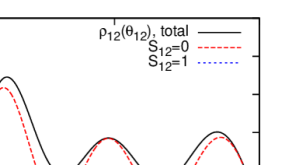
(a) (c) (b) (d)

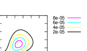
Figure 4.2: The two-nucleon density distribution of ¹⁸Ne, $\rho$, calculated for the ground state within the three-body model. Those are plotted for several sets of coordinates as follows. (a) with $r_{\rm N-N}$ and $r_{\rm c-NN}$. (b) with $r_{\rm N-N}$, integrated for $r_{\rm c-NN}$. (c) with the opening angle $\theta_{12}$ between the valence nucleons, integrated for $r_{1}$ and $r_{2}$. (d) with $r_{1}$ and $r_{2}$, integrated for $\theta_{12}$. In panel (d), the radial weight $r_{1}^{2}r_{2}^{2}$ is omitted to emphasize the peak(s).

“18O (g.s.)”

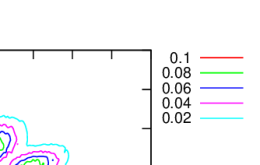
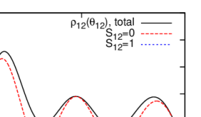
(a) (c) (b) (d)

Figure 4.3: The same to Figure 4.2 but of ¹⁸O.

In Figure 4.2, we show the density distribution of ¹⁸Ne, plotted within several sets of coordinates. In panel (a), $\rho(r_{1},r_{2},\theta_{12})$ is plotted as a function of the relative distances, $r_{\rm N-N}$ and $r_{\rm c-NN}$ given by Eqs.(4.15) and (4.16). In panel (b), this function is integrated for $r_{\rm c-NN}$, and plotted only with $r_{\rm N-N}$. Conversely, in panel (c), we integrate $\rho$ for $r_{1}$ and $r_{2}$, and plot it as a function of the opening angle, $\theta_{12}$. We also plot the spin-singlet and triplet components separately in this panel. Finally, in panel (d), we integrate $\rho$ for the opening angle, and plot it as a function of $r_{1}$ and $r_{2}$. In this plotting, in order to clarify the peak(s), we omit the radial weight, $r_{1}^{2}r_{2}^{2}$ in Eq.(4.23). We show similar plots for ¹⁸O in Figure 4.3.

As general aspects, from Figures 4.2, 4.3 and Table 3, we can see the similarity of the two-nucleon configurations in ¹⁸Ne and ¹⁸O, consistently to the similarity shown in Table 2. It means that the reduction of pairing energies caused by the Coulomb repulsion, which is evaluated as about $-10$% reduction, does not affect significantly the two-nucleon densities. Because of the weakly binding due to Coulomb repulsions, the density of ¹⁸Ne is slightly extended compared with ¹⁸O. This tendency is intuitively understood by comparing Figs. 4.2(b),(d) and 4.3(b),(d). Correspondingly, the expectation values of distances in the 1st-4th rows of Table 3 show larger values in the case of ¹⁸Ne. It is also shown from the probabilities of the angular channels that the $(d_{5/2})^{2}$ wave is dominant in both two cases, whereas the $(s_{1/2})^{2}$ wave has also considerable contributions. The distinct three peaks in panels (a) and (c) are mainly due to the $(d_{5/2})^{2}$ component, although the mixing of the other waves occurs with the pairing correlations, where the Coulomb repulsion plays a minor role.

We note that the mean distance between the two nucleons, $r_{\rm N-N}$, shows a considerably smaller value, compared with the total diameter of the whole nucleus, estimated as $\simeq 2r_{\rm c-NN}\simeq 5.5$ fm.

4.1.6 Diproton and Dineutron Correlations

In the ground states of both ¹⁸Ne and ¹⁸O, the dinucleon correlation, or at least, its tendency can be seen. The spatial localization is apparent at ($r_{\rm N-N},r_{\rm c-NN}$) $\simeq$ (2fm, 3fm) in Figs. 4.2(a) and 4.3(a). It corresponds to the two nucleons confined in $r_{\rm N-N}\leq 2$ fm, which corresponds to the first peak of $\rho_{12}(r_{\rm N-N})$ shown in Figs. 4.2(b) and 4.3(b). We also find that $\rho_{12}(r_{\rm N-N})$ has almost all the components inside $r_{\rm N-N}\leq 8$ fm. According to the Ref.[18], this result may be connected to the pairing densities in the nuclear matter at $\rho/\rho_{0}=0.1-0.01$ (see Fig.2.4), even though the assumption of nuclear matters cannot be translated directly to the conditions in finite nuclei.

In Figs. 4.2(c) and 4.3(c), the corresponding angular distributions take the asymmetric forms, and have the highest peak at the small opening angle, $\theta_{12}\simeq\pi/6$. Indeed, this asymmetry is an important character of the dinucleon correlations: it is caused by the mixing of different parities of the core-nucleon partial system [90]. If we exclude this parity-mixing, the angular distributions have the perfect symmetric forms. We will check this point in the next section.

We also note that in the asymmetric angular distributions, the most localized peak is mainly from the spin-singlet configuration, consistently to the definition of the dinucleon correlations. In both two nuclei, the spin-singlet has a probability of about 80%. On the other hand, if we take the naive mean-field approximation, the two nucleons have the pure $(d_{5/2})^{2}$ wave, where the contribution from the spin-singlet is determined exactly as 60% from the properties of the CG and the $9j$-coefficients. Thus, the pairing correlation works to enhance the spin-singlet configuration compared to the pure $(d_{5/2})^{2}$ wave.

As interim conclusions, we have confirmed that the diproton correlation, which is characterized as the spatial localization of two-proton density mainly carried out by the spin-singlet configuration, is able to occur similarly to the dineutron correlation in the mirror nucleus. This result is consistent to the minor effect of the Coulomb repulsion, estimated by about -10% reduction of the pairing energy.

4.2 Diproton Correlation in ¹⁷Ne

In the previous section, it has been suggested that the structural properties of the two nucleons are insensitive to the total binding energy. In order to investigate the dependence of the dinucleon correlations on the binding energy, we next study the ¹⁷Ne nucleus, which has been famous as a 2p-Borromean nucleus. This nucleus is also a candidate to have the 2p-halo structure, due to the loosely bound two protons [122, 126]. In this system, two valence protons are bound with significantly small binding energies, $S_{\rm 2p}=0.93$ MeV [153]. Therefore, it provides another testing ground to investigate the diproton correlation in a weakly bound system, in comparison with the diproton correlation in a deeply bound nucleus, ¹⁸Ne. In this section, we will also perform case-studies with different theoretical conditions, in order to gain a deeper understanding of the diproton correlation. Although these theoretical conditions may not correspond to realistic situations, those will be helpful to know what is the essential point in the diproton and dineutron correlations.

4.2.1 Set up for Calculations

It is known that there is no bound state in ¹⁶F $\cong^{15}$O+p, but four resonances in the low-lying region. These low-lying levels are shown in Figure 4.4. The ground state of ¹⁵O has $1/2^{-}$, whereas its first excited state is located at $5.18$ MeV above the ground state. Because this excited energy is sufficiently high, the first and the second low-lying resonances in ¹⁶F at 0.536 and 0.729 MeV can be interpreted as the coupled states of ¹⁵O${}_{g.s.}(1/2^{-})$+$p(s_{1/2})$. Likewise, the 3rd and the 4th resonances at 0.960 and 1.257 MeV can be interpreted as those of ¹⁵O${}_{g.s.}(1/2^{-})$+$p(d_{5/2})$.

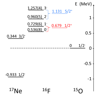
Figure 4.4: The level scheme of the ¹⁷Ne nucleus and its isotones. All the experimental values, printed by black letters, are quoted from the database [153], except for the first excited state of ¹⁷Ne [119]. For the decay widths of ¹⁶F, the experimental data are $\Gamma(0^{-})=40\pm 20$ keV and $\Gamma(1^{-})<40$ keV for the lower two levels, whereas $\Gamma(2^{-})=40\pm 30$ keV and $\Gamma(3^{-})<15$ keV for the upper two levels [153]. Note that all these levels decay via one-proton emission, where the branching ratios to other decay-modes are negligible. The values printed by the red and blue letters for ¹⁶F indicate the spin-averaged s.p. energies. The decay widths of these levels are theoretically computed as $\Gamma_{0}(s_{1/2})=63$ keV and $\Gamma_{0}(d_{5/2})=8.2$ keV, respectively.

In this case, we neglect the internal spin of the core, and fit the parameters in the core-proton potential to the spin-averaged s.p. energies of $(s_{1/2})$ and $(d_{5/2})$ states. These averaged levels are shown in Figure 4.4 by the red and blue letters. To this end, we calculate the phase shift, $\delta_{lj}(E)$, and its derivative for the energy $E$. The calculated result is fitted with a function, which consists of a pure Breit-Wigner distribution and a smooth background. That is,

$$\frac{d\delta_{lj}(E)}{dE}=\frac{\Gamma_{0}/2}{\Gamma_{0}^{2}/4+(E_{0}-E)^{2}}+\frac{dC_{lj}(E)}{dE},$$ (4.32)

where the right-hand side is the empirical formula. How to derive Eq.(4.32) and calculate $\delta_{lj}(E)$ in the left-hand side is summarized as Appendix D.

The calculated results and fitted functions are shown in Figure 4.5. At this moment, the smooth background is neglected. By fitting the right-hand side in Eq.(4.32) to the calculated left-hand side, we can extract the resonant energy, $E_{0}$ and the decay width, $\Gamma_{0}$ of considering resonances. With $r_{0}=1.22$ fm, $a_{\rm core}=0.65$ fm, $V_{0}=-53.68$ MeV and $V_{ls}=15.06$ ${\rm MeV\cdot fm^{2}}$ for the ¹⁵O-proton potential, we obtained $E_{0}=0.679$ MeV with $\Gamma_{0}=63$ keV for the $(s_{1/2})$-resonance, and $E_{0}=1.131$ MeV with $\Gamma_{0}=8.2$ keV for the $(d_{5/2})$-resonance. Obtained values of $E_{0}$ are consistent with the empirical resonant energies shown in Fig. 4.4. Notice that the values of $r_{0}$ and $a_{0}$ are similar to those used for ¹⁸Ne and ¹⁸O. The other s.p. states are also solved within this potential.

“$d\delta_{lj}/dE$ of 15O-proton”

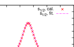
(a) for $(s_{1/2})$ (b) for $(d_{5/2})$

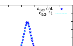
Figure 4.5: The derivative of the phase shift, $\delta_{lj}(E)$ for the energy $E$ in the scattering of ¹⁵O-proton. The calculated results are shown with symbols, whereas the fitted functions given by Eq.(4.32) are plotted with lines.

In order to solve the ground state of ¹⁷Ne, we employed the similar setting to that for ¹⁸Ne and ¹⁸O. Namely, we take all the s.p. states up to $l_{\rm max}=5$ into account. Since the ground state of ¹⁷Ne has the same spin-parity to ¹⁵O, which is $(1/2^{-})$, the two-proton uncorrelated basis can be reduced only to the $0^{+}$ subspace. Consequently, we adopt from $(s_{1/2})^{2}$ to $(h_{11/2})^{2}$ partial waves. We use $\epsilon_{a}+\epsilon_{b}\leq E_{\rm cut}=30$ MeV as the energy cutoff for the uncorrelated basis, providing about 360 bases. For the pairing interaction, except for $v_{\rho}$ in the density-dependent part, we adopt the same parameters as those for ¹⁸Ne and ¹⁸O. In order to reproduce the empirical binding energy of the two protons, $S_{\rm 2p}=0.93$ MeV [153], we use $v_{\rho}=-1.131v_{0}$.

In the setting of the calculations introduced above, we treat the pairing correlations as fully as possible, by mixing all the uncorrelated bases up to $(h_{11/2})^{2}$. We often refer to this condition as “full-mixing” or just “full” in the following. In addition to this “full-mixing” case, we perform two other sets of calculations with different conditions explained below, which reveal the essential aspect of the dinucleon correlations.

• Limitation of Core-proton Parity:
  As shown in Table 3, the contributions from the partial waves with $(l=odd)^{2}$ are quite small in ¹⁸Ne and ¹⁸O. This situation is expected to occur also in ¹⁷Ne, where the two protons may mainly have the $(d_{5/2})^{2}$ and $(s_{1/2})^{2}$ configurations. Thus, we examine the case by excluding the $(l=odd)^{2}$ partial waves from the calculation, for comparison with the full-mixing case. It corresponds to a situation where the parity-mixing in the partial core-proton system is prohibited. In order to reproduce the 2p-binding energy, we tune the parameter $v_{\rho}$ as $v_{\rho}=-0.9981v_{0}$. It meas that, without the parity mixing, we need a stronger pairing attraction than that in the full case. Notice also that the recoil term, which couples two bases satisfying $\left|l^{\prime}-l\right|=1$, do not contribute in this case (see Eq.(3.70) also). In the following, we call this setting as “$(l=even)^{2}$” case.

• No Pairing:
  In this case, we completely omit the pairing correlations. It means that we ignore all the nuclear attraction, the Coulomb repulsion and the recoil term between the two protons in Eq.(3.1). Thus, the total Hamiltonian is only the uncorrelated Hamiltonian, $h_{1}+h_{2}$, and the two-proton wave functions becomes identical to one of the uncorrelated bases with single angular channel. We take the $(d_{5/2})^{2}$ state, which is expected to be the major channel in the full-mixing case. Because of the lack of the pairing correlations, we cannot reproduce the empirical binding energy, $S_{\rm 2p}=0.93$ MeV, with the original core-proton interaction used in the “full” and “$(l=even)^{2}$ only” cases. Therefore, we inevitably modify $V_{\rm c-N}$. We use $V_{0}=-57.663$ MeV, which yields the bound s.p. state in the $(d_{5/2})$ channel with $\epsilon(d_{5/2})\simeq-0.93/2$ MeV. Notice that it is no longer possible to reproduce the Borromean character in this case. In the following, we call this setting as “no pairing”.

By comparing among these three cases, we will make an attempt to extract the essential character of the dinucleon correlation. The results and discussions are summarized below.

4.2.2 Energy Expectation Values

We first discuss the energetic properties tabulated in Table 4. In the full-mixing case, these expectation values show similar results to those for ¹⁸Ne shown in Table 2, except for $\Braket{h_{1}+h_{2}}$ and $\Braket{h_{\rm c-NN}}$. This difference can be interpreted as an effect of the weak attractive potential in the core-proton subsystem. On the other hand, it is implied that the effects of the pairing correlations, as well as the relative energy between the two protons, are not significantly dependent on the total binding energy. The effect of the Coulomb repulsion in the pairing correlation is estimated again as a $10\%$ reduction over the nuclear attraction. These conclusions are similar to those obtained in Sec. 4.1.

In the $(l=even)^{2}$ case, the situation is significantly different. Even though we employ a stronger pairing attraction than in the full case, the pairing energy, $\Braket{v_{\rm N-N}}$ has a higher value. On the other hand, the expectation value of the energy of the proton-proton subsystem, $\Braket{h_{\rm N-N}}$ becomes lower. Consequently, the relative proton-proton kinetic energy, $\Braket{p^{2}_{\rm N-N}/2\mu_{\rm N-N}}=\Braket{h_{\rm N-N}}-\Braket{v_{\rm N-N}}>0$, has the lower value than that in the full-mixing case. The lower value of $\Braket{p^{2}_{\rm N-N}/2\mu_{\rm N-N}}$ suggests that the spatial distribution between the two protons is further expanded, and possibly deviated from a diproton-like configuration.

Finally, in the no pairing case, it is worthwhile to point out that $\Braket{h_{\rm N-N}}$ and $\Braket{h_{\rm c-NN}}$ have similar values to those in the full case. From this result, one may infer that the pairing correlations are well mocked up in the mean-field, $V_{\rm c-N}$. However, compared with the full-mixing case, a discussion on the 2p-configuration is not straight forward, because the modification of $V_{\rm c-N}$ makes the proton-proton subsystem considerably different in the two cases. Thus, we will check directly the difference in the spatial 2p-distributions in the next subsection.

		17Ne
		full	$(l=even)^{2}$ only	no pairing, deeper $V_{\rm c-p}$
$\Braket{H_{\rm 3b}}=-S_{\rm 2N}$ (MeV)		$-0.93$	$-0.93$	$-0.93$
$\Braket{v_{\rm N-N}}$ (MeV)		$-4.00$	$-3.86$	$\phantom{0}\phantom{0}0.\phantom{0}\phantom{0}$
$\Braket{v_{\rm N-N,Nucl.}}$ (MeV)		$-4.53$	$-4.34$	$\phantom{0}\phantom{0}0.\phantom{0}\phantom{0}$
$\Braket{v_{\rm N-N,Coul.}}$ (MeV)		$\phantom{0}\phantom{0}0.53$	$\phantom{0}\phantom{0}0.48$	$\phantom{0}\phantom{0}0.\phantom{0}\phantom{0}$
$\Braket{\rm recoil}$ (MeV)		$-0.40$	$\phantom{0}\phantom{0}0.\phantom{0}\phantom{0}$	$\phantom{0}\phantom{0}0.\phantom{0}\phantom{0}$
$\Braket{h_{1}+h_{2}}$ (MeV)		$\phantom{0}\phantom{0}3.47$	$\phantom{0}\phantom{0}2.93$	$-0.93$
$\Braket{V_{\rm c-N_{1}}+V_{\rm c-N_{2}}}$ (MeV)		$-10.64$	$-11.75$	$-12.82$
$\Braket{h_{\rm N-N}}$ (MeV)		$\phantom{0}\phantom{0}5.61$	$\phantom{0}\phantom{0}3.02$	$\phantom{0}\phantom{0}5.57$
$\Braket{h_{\rm c-NN}}$ (MeV)		$-6.54$	$-3.95$	$-6.50$

Table 4: The energy expectation values for the ground state of ¹⁷Ne, calculated with the three-body model of ¹⁵O+p+p. See the text for the details of each calculational setting. The experimental two-proton separation energy is $S_{\rm 2p}=0.93$ MeV [153]. All quantities are evaluated in the same manner as in Table 2.

4.2.3 Structural Properties

The results for the structural properties of ¹⁷Ne are shown in Table 5 and Figs. 4.6, 4.7 and 4.8. All the quantities are evaluated and plotted in the same manner as those in Table 3 and Figure 4.2.

		17Ne
		full	$(l=even)^{2}$ only	no pairing, deeper $V_{\rm c-p}$
$\sqrt{\Braket{r^{2}_{1}}}=\sqrt{\Braket{r^{2}_{2}}}$ (fm)		3.92	3.70	3.67
$\sqrt{\Braket{r^{2}_{\rm N-N}}}$ (fm)		4.98	5.24	5.20
$\sqrt{\Braket{r^{2}_{\rm c-NN}}}$ (fm)		3.03	2.62	2.60
$\Braket{\theta_{12}}$ (deg)		81.2	90.0	90.0
$(s_{1/2})^{2}$ (%)		14.63	13.24	000.0
$(d_{5/2})^{2}$ (%)		77.97	82.64	100.0
$(p_{3/2})^{2}$ (%)		00.79	00.00	000.0
$(p_{1/2})^{2}$ (%)		00.23	00.00	000.0
others,$(l=evev)^{2}$ (%)		03.87	04.12	000.0
others,$(l=odd)^{2}\phantom{0}$ (%)		02.51	00.00	000.0
$P(S_{12}=0)$ (%)		82.62	82.39	60.00

Table 5: The structural properties in the ground state of ¹⁷Ne, calculated with the three-body model of ¹⁵O+p+p. See the text for the details of each calculational setting. The radius of the core nucleus is estimated as $R_{0}=r_{0}A_{c}^{1/3}=1.22\cdot 15^{1/3}\cong 3.009$ fm.

In the full-mixing case, we first find that the general features of ¹⁷Ne are similar to those of ¹⁸Ne, although the binding energy is remarkably smaller. This smaller energy yields the sizable extension of the 2p-density distribution, shown in Figs. 4.6(a), (b) and (d). Consequently, the expectation values of the radial parameters become larger as one can see in Table 5. This extension of the 2p-wave function is consistent to an increment of the $(s_{1/2})^{2}$ wave, which has a long tail outside the core-nucleon potential. We also stress that the major components in the 2p-wave function are $(s_{1/2})^{2}$ and $(d_{5/2})^{2}$, reflecting the existence of the $(s_{1/2})$- and $(d_{5/2})$-resonant states in the core-proton subsystem. The dominance of the $(d_{5/2})^{2}$ wave in the ground state can be understood from Eq.(3.57), which indicates that the matrix element of a coupled operator, $O(\xi_{1},\xi_{2})$, has a larger value for the uncorrelated basis with larger $j$. Therefore, to gain a deeper binding energy, the two protons tend to occupy the $(d_{5/2})^{2}$.

“17Ne (g.s.), $v_{\rm N-N}=$DDC+Coul., full-mixing”

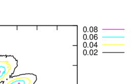
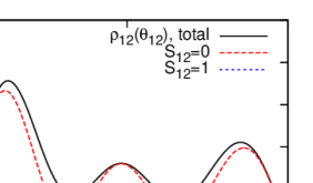
(a) (c) (b) (d)

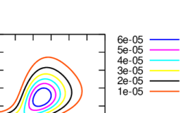
Figure 4.6: The density distribution of the valence two protons in ¹⁷Ne, computed with the three-body model of ¹⁵O+p+p. In this case, all the uncorrelated bases up to $(h_{11/2})^{2}$ are fully taken into account (the full-mixing case). The coordinates for all the panels are defined in a similar way as Figure 4.2.

In order to discuss the diproton correlation, it is useful to compare the results obtained with the three settings for calculations. First, in panels (a), (b) and (c) of Fig. 4.6 for the full-mixing case, the localization of the density at small values of $r_{\rm p-p}$ and of $\theta_{12}$ can be seen, whereas the localization cannot be observed in both Fig. 4.7 for the $(l=even)^{2}$ only case and Fig. 4.8 for the no-pairing case. Notice that this localization in the full-mixing case is mainly due to the spin-singlet configuration, as shown in Fig. 4.6(c). This implies the existence of the diproton correlation, or at least, its tendency in the ground state of weakly bound ¹⁷Ne.

We also point out that the spatial localization of the two protons in ¹⁷Ne is less significant than that in ¹⁸Ne. For example, by comparing panels (b) and (d) in Figs. 4.2 and 4.6, one can find that the 2p-density distribution shows a larger extent in ¹⁷Ne. The expectational values, $\Braket{r_{N-N}}$ and $\Braket{\theta_{12}}$, also have larger values in ¹⁷Ne. This result can be interpreted as the effect of the density-dependence of the pairing correlation. If the density is too low, the pairing correlation decreases, and eventually vanishes in the zero-density limit [18]. In ¹⁷Ne, the valence two protons possibly feel the surrounding density, which is rather low due to the weakly bound system, and causes the diproton correlation to be weaker. Whether this tendency leads to the reduction of the diproton correlation from unbound systems or not will be a critical point when we analyze 2p-emissions. We will discuss this point in Chapter 7.

“17Ne (g.s.), $v_{\rm N-N}=$DDC+Coul., $(l=even)^{2}$ only”

(Figure is hidden in open-print version.)

Figure 4.7: The same as Figure 4.6 but for the $(l=even)^{2}$ case.

“17Ne (g.s.), no pairing”

(Figure is hidden in open-print version.)

Figure 4.8: The same as Figure 4.6 but without the pairing correlations, for which a modified core-proton potential is employed. Notice that the two protons have a pure $(d_{5/2})^{2}$ configuration.

In the $(l=even)^{2}$ case, the density $\rho_{12}(r_{\rm N-N})$ shown in Fig. 4.7(b) shows a larger extent than that in the full case. This is consistent with the larger value of $\sqrt{\Braket{r^{2}_{\rm N-N}}}$ in Table 5. The angular distribution in Fig. 4.7(c) has a completely symmetric form, yielding $\Braket{\theta_{12}}=90$ (deg). From these results, we can conclude that the parity-mixing in the core-nucleon subsystem is indispensable to induce the spatial localization of two nucleons. In other words, if this parity-mixing is forbidden or excessively suppressed, two nucleons cannot be localized even with a strong pairing interaction.

One should remember that, even though the two protons are not localized, the $(l=even)^{2}$ case does not mean the complete lack of the pairing correlations. In Table 5, the enhancement of the spin-singlet configuration can be seen, as well as in the full-mixing case. Comparing Fig. 4.7(c) with Fig. 4.8(c), one can find that the peaks at $\theta_{12}\simeq\pi/6$ and $5\pi/6$ become more significant in the $(l=even)^{2}$ case than those in the no pairing case. These show that a part of the pairing correlations is taken into account, even though the diproton correlation is missing.

4.3 Interaction-Dependence of Diproton Correlation

It is also useful to check a model-dependence of the results in the previous section, which showed the possibility of the dinucleon correlations in weakly bound systems. In order to clarify this point, in this section, we repeat the same calculations for ¹⁷Ne, but employing a different pairing interaction.

4.3.1 Minnesota Potential

To this end, we adopt the “Minnesota potential” for the pairing interaction instead of the DDC potential. This potential was originally proposed by Thompson et.al., in order to solve nucleon-nucleus scattering problems within the microscopic “resonating group method” [154]. For the proton-proton and the neutron-neutron systems, the potential is given as

$$v_{\rm N-N}(r_{12})=v_{0}e^{-b_{0}r^{2}_{12}}-v_{1}e^{-b_{1}r^{2}_{12}}+\alpha\hbar c\frac{e^{2}}{r_{12}}\frac{(1+\hat{t}^{(3)}_{1})(1+\hat{t}^{(3)}_{2})}{4},$$ (4.33)

with $r_{12}\equiv\left|\bm{r}_{1}-\bm{r}_{2}\right|$ and $\alpha$ is the fine structure constant. The Coulomb part is necessary only in the proton-proton case. For this interaction, the nuclear part has finite rages, in contrast to the zero-range DDC pairing. The first term is a phenomenological repulsive part, whereas the second term describes the pairing attractions. The original parameters in Eq.(4.33) were given as

$$v_{0}=200.~{}{\rm MeV},~{}~{}~{}~{}~{}b_{0}=1.487~{}{\rm fm}^{2},$$ (4.34)

for the repulsive part, whereas

$$-v_{1}=\left\{\begin{array}[]{cc}-178.~{}{\rm MeV},&(S_{12}=0)\\ -91.85~{}{\rm MeV},&(S_{12}=1)\end{array}\right.~{}~{}~{}~{}~{}b_{1}=\left\{\begin{array}[]{cc}0.639~{}{\rm fm}^{2},&(S_{12}=0)\\ 0.465~{}{\rm fm}^{2},&(S_{12}=1)\end{array}\right.$$ (4.35)

for the attraction, which depends on the total spin of the two nucleons. In Eq.(4.35), the parameters for the spin-singlet configuration were determined so as to reproduce the proton-proton, spin-singlet, $s$-wave scattering properties. On the other hand, for the spin-triplet configuration, those parameters were determined consistently to the neutron-proton, spin-triplet, $s$-wave scattering properties . In several theoretical studies based on few-body models for finite nuclei, the Minnesota potential has been employed with reasonable successes [154, 33, 155, 135, 156]. In Figure 4.9, the potentials for the proton-proton and the neutron-neutron channels are shown.

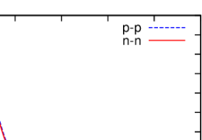
(a) $S_{12}=0$ (b) $S_{12}=1$

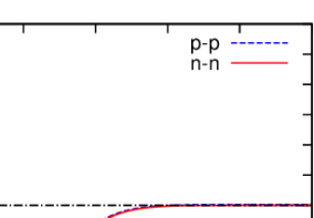
Figure 4.9: The original Minnesota potentials in the $S_{12}=0$ (the left panel) and the $S_{12}=1$ (the right panel) channels. In the proton-proton case, the Coulomb term is also included. The dashed curves are for the proton-proton, while the solid lines are for the neutron-neutron.

In our calculations for ¹⁷Ne, however, the original set of parameters underestimates the empirical 2p-separation energy. We thus weaken $v_{0}$ to $178.1$ MeV, which effectively enhances the pairing attraction. One should be conscious of that, in this case, a stronger pairing attraction is adopted inside nuclei, compared with the bare pairing attraction in the vacuum. It is quite contrary to the previous case with the DDC pairing interaction, where we needed to reduce the pairing attraction inside nuclei to reproduce the 2p-binding energy. We do not know exactly the origin for the difference, but one possibility is due to the range of the pairing attraction.

To calculate the matrix elements of the Minnesota potential based on Eq.(3.57), we have to know the multi-pole expansion formula of the Gaussian function. This was given by Swiatecki [157], and thus we do not show it here. We stress that, except using the Minnesota pairing, our calculations were performed within the same assumption to that in the full mixing case with DDC pairing.

4.3.2 Results and Comparison

The results obtained with the Minnesota pairing are summarized in Table 6 and Figure 4.10, in the same manner as in the previous section. Qualitatively, energy expectational values are independent of the choice of the pairing interaction. Indeed, $\Braket{v_{\rm N-N,Nucl.}}$ is similar to one another, even it is evaluated slightly lower than that in the DDC+Coul. case, which maybe due to a character of the finite-range potential.

17Ne (g.s.), $v_{\rm N-N}=$Minne.+Coul., full-mixing

$\Braket{H_{\rm 3b}}=-S_{\rm 2N}$ (MeV) $-0.93$ $\Braket{v_{\rm N-N}}$ (MeV) $-3.52$ $\Braket{v_{\rm N-N,Nucl.}}$ (MeV) $-4.03$ $\Braket{v_{\rm N-N,Coul.}}$ (MeV) $\phantom{0}\phantom{0}0.51$ $\Braket{\rm recoil}$ (MeV) $-0.31$ $\Braket{h_{1}+h_{2}}$ (MeV) $\phantom{0}\phantom{0}2.90$ $\Braket{V_{\rm c-N_{1}}+V_{\rm c-N_{2}}}$ (MeV) $-11.1$ $\Braket{h_{\rm N-N}}$ (MeV) $\phantom{0}\phantom{0}5.41$ $\Braket{h_{\rm c-NN}}$ (MeV) $-6.34$

$\sqrt{\Braket{r^{2}_{1}}}=\sqrt{\Braket{r^{2}_{2}}}$ (fm) 3.81 $\sqrt{\Braket{r^{2}_{\rm N-N}}}$ (fm) 4.95 $\sqrt{\Braket{r^{2}_{\rm c-NN}}}$ (fm) 2.89 $\Braket{\theta_{12}}$ (deg) 83.37 $(s_{1/2})^{2}$ (%) 12.12 $(d_{5/2})^{2}$ (%) 84.99 $(p_{3/2})^{2}$ (%) 00.42 $(p_{1/2})^{2}$ (%) 00.10 others,$(l=evev)^{2}$ (%) 00.82 others,$(l=odd)^{2}\phantom{0}$ (%) 01.55 $P(S_{12}=0)$ (%) 72.73

Table 6: The properties of the ground state of ¹⁷Ne, obtained with the Minnesota interaction. All the uncorrelated bases up to $(h_{11/2})^{2}$ are taken into account. All the quantities are evaluated in a similar way as in Table 4 and 5.

Even though the relative proton-proton energy is less evaluated with the Minnesota potential, the tendency of the diproton correlation can be apparent again in this case. The structural properties shown in Table 6 and the 2p-density distribution shown in Figure 4.10 exhibit the similar behaviors to those in the DDC+Coul. case. The spatial localizations at $r_{\rm p-p}\simeq 2$ fm in Fig. 4.10(a), and at $\theta_{12}\simeq\pi/6$ in Fig. 4.10(c) are clearly seen by taking the core-proton parity-mixing into account. The spin-singlet configuration carries the main part of this localization as one can see in Fig. 4.10(c). One may concern the spin-singlet ratio which is slightly smaller than that in the DDC+Coul. case. However, it is significantly larger than $P(S_{12}=0)=60$ % in the no pairing case, and the enhancement of the spin-singlet configuration remains qualitatively also with the Minnesota potential.

“17Ne (g.s.), $v_{\rm N-N}=$Minne.+Coul., full-mixing”

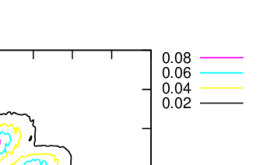
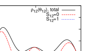
(a) (c) (b) (d)

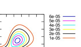
Figure 4.10: The same as Figure 4.6, but obtained with the Minnesota interaction.

4.4 Summary of this Chapter

We demonstrated the appearance of the dinucleon correlations in the ground states of several light nuclei based on the core plus two-nucleon model. It is found that the Coulomb repulsive force plays a minor role in the pairing correlation, and the diproton correlation can be realized in proton-rich nuclei, in a similar way as the dineutron correlation in neutron-rich nuclei. That is, our evaluation of the Coulomb effect, which is about a 10% reduction against the nuclear pairing attraction, is not sufficient to affect the spatial localization of the two protons. We also confirmed that these correlations are not significantly dependent on the total binding energy of nuclei. In other words, the dinucleon correlations are present not only in weakly bound but also in stable nuclei, as long as the pairing correlation is sufficiently large.

As mentioned in Chapter 2, the dinucleon correlations in the bound, ground states are not easy to be directly probed. The sensitivity of observables to these intrinsic structures is still not evident, although various possibilities have been explored. Facing on this situation, we propose a possibility to verify the diproton correlation with the two-proton emissions and radioactive decays. Because the valence two protons are spontaneously emitted without no disturbance from the external fields, observing their wave functions may be a direct probe into the diproton correlation in a resonant state. Based on this idea, we will extend our analysis to a meta-stable three-body system after this Chapter. In the next Chapter, we will summarize the historical back-ground of the two-proton emissions and radioactive decays. We will introduce the time-dependence into our three-body model in order to describe the two-proton emissions in Chapter 6. Employing this model, we will the diproton correlation associated with the two-proton emissions, whose results will be present in Chapters 7 and 8.

Chapter 5 Review of Two-Proton Decay and Emission

The two-proton decay and emission are characteristic decay-modes of nuclei beyond the proton-dripline. We review in this Chapter the theoretical and experimental studies of these phenomena, with their relevant topics.

In nuclear physics, there have been five major radioactive processes in which one or several nucleons are emitted from the parent nuclei . Those are (i) alpha decay, (ii) one-proton and one-neutron decays, (iii) two-proton and two-neutron decays, (iv) heavier cluster decay, and (v) nuclear fission. All these processes belong to the quantum meta-stable phenomena by the nuclear interaction.

Needless to say, the alpha-decay is one of the most famous nuclear radioactive processes. In many standard textbooks of nuclear physics, this problems is discussed as an tunneling problem of a point-like alpha-particle. However, it is also known that the emitted alpha-particle is a composite system of four nucleons. Therefore, to describe the alpha-decay properly, one would need a microscopic framework including many-body effects. There have been several theoretical studies based this consideration [158, 159, 160, 161]. However, mainly because of a difficulty to handle with many-body correlations, there have been no quantitatively successful works yet. We also note that the physics of meta-stable states with intrinsic degrees of freedom, or of many particles are one of the major subjects in modern physics. They occupy the essential positions not only in nuclear physics, but also in molecular, condensed matter and astro-nuclear physics. Famous examples include, e.g. nuclear fissions and fusions, resonances of cold atoms and Jossefson effects. A unified study of multi-fermion meta-stable systems in different scales might be useful in gaining a deeper understanding of our world.

In the following, we mainly focus on the 2p-decay and emission, whereas other processes will be briefly or never mentioned. In these processes, two protons are emitted simultaneously or sequentially from the parent nucleus with an even-number of protons. Because of the remarkable developments in the experimental techniques [45, 142, 47, 46], for recent about 10 years, two-proton (2p-) emitters have been one of the main topics in radioactive nuclear physics, and knowledge about 2p-emissions and radioactive decays have been accumulated. Recently, furthermore, the two-proton (2p-) emission has attracted much attention as an useful tool to probe the diproton correlation. We detail this history in the following.

5.1 History of Two-Proton Decay and Emission

Comparing with alpha-decays and fissions, the two-proton emissions and decays are much simpler. Moreover, those are the dynamical phenomena, including the pairing correlations which are unique in multi-fermion systems. By studying 2p-decays, it has been expected to provide the benchmark for the quantum meta-stability of many fermions.

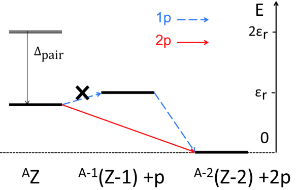
(a) true 2p-emitter (b) sequential 2p-emitter

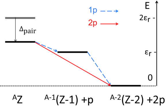
Figure 5.1: Schematic figures for the energy conditions of the true 2p-emitters (the left panel) and the sequential 2p-emitters (the right panel). The parent nucleus is indicated as ${}^{A}Z$. Each level is measured from the ground state of the daughter nucleus, ${}^{A-2}(Z-2)$. It is assumed that there are no bound $1p$- and $2p$-states in the ${}^{A-1}(Z-1)$ and ${}^{A}Z$ nuclei, respectively. The symbol $\Delta_{\rm pair}$ means the pairing energy gap due to the pairing attraction. The decay widths are not considered in these schematic figures.

5.1.1 Early Studies: before the 21th Century

The first prediction of 2p-decays was done by V. I. Goldansky [67, 68]. In his theoretical study, he considered two different, simple situations for 2p-emissions: “true” and “sequential” 2p-emitters. In Fig. 5.1, we schematically describe these two situations, as the energy conditions for a parent nucleus with respect to the nuclei after $1p$- and 2p-emissions.

In the true 2p-emitter, the energy pf the 2p-resonance of a parent nucleus is lower than the $1p$-resonance of its isotone after the $1p$-emission. In this situation indicated in Fig. 5.1(a), only the simultaneous 2p-emission is allowed, whereas the emission of single proton is forbidden. In the pure mean-field approximation, this situation is never realized as long as the intermediate nucleus, ${}^{A-1}(Z-1)$, has no bound single-proton states: the 2p-resonance has the energy of $2\epsilon_{r}$, where the $\epsilon_{r}>0$ is the single-proton resonance energy in the intermediate nucleus. Thus, in order to realize the true 2p-emission, the pairing energy gap must be large enough to pull down the 2p-resonance under the single-proton resonance. This energy gap is, of course, caused by the pairing interaction. Based on the quasi-classical formulas, Goldansky showed that, in the true 2p-emission, the decay width is sharply reduced from that of common binary decays [67, 68].

In Goldansky’s pioneer works, he proposed two types of the true 2p-emissions. The first one is “diproton” emission: if the pairing attraction is much stronger than the Coulomb repulsion, two protons are emitted almost as a diproton. He showed that, in the case of two protons restricted to the relative $(s_{1/2})$-orbit from the core, the penetrability is identical to that of a diproton with the total spin $S=0$. This observation has been a basic idea of the diproton emission. On the other hand, he also proposed “direct” emission, where the pairing correlation is rather weak. In the direct 2p-emission, the observables are mainly governed by the core-proton interactions, where the disruption by the pairing interaction can be negligible (Notice that even if the pairing energy gap is large enough, the effect of pairing correlations may be minor for the emitted particles). Consequently, the diproton and direct decays or emissions correspond to the extreme conditions with relatively strong and weak pairing correlations, respectively. The binary channel of the proton-proton and the core-proton plays a dominant role in the diproton and the direct emissions, respectively.

However, it is important to notice that the actual true 2p-emissions are not so simple that they usually show an intermediate character between the diproton and direct emissions. It is often necessary to deal with three particles without any discrimination. This process is referred to as “democratic” emission [55, 47, 57], where there are no autocrat binary channels. Namely, the actual true 2p-emissions are essentially the three-body problems, and they cannot be approximated as the product of partial two-body problems.

In the sequential 2p-emitter indicated in Fig. 5.1(b), on the other hand, the $1p$-emission becomes dominant in a parent nucleus. This situation can be understood by the mean-field plus a small pairing gap, which is insufficient to realize the true 2p-emission. Thus, the decay process to the final daughter nucleus occurs as a sequence of two $1p$-emissions. According to this picture, sometimes the process is also called “cascade” decay. In the sequential 2p-emissions, of course, the pairing correlations should be minor. Observables are almost explained only with the core-proton interactions. The total penetrability should be well approximated as the bi-product of the penetrabilities for the first and second protons. However, one should also notice that the direct 2p-emission can takes place also in this situation, if the first and second $1p$-emissions occur at the same time.

After Goldanski’s works, these three types of $2{\it p}$-emissions have been the major assumptions in almost all the theoretical works [162, 163, 164, 165]. We also note that there were less theoretical works before 2000. The reason for this poor crop may be a shortage of observed examples of 2p-emitters, which can be analyzed within the theoretical models in those days.

In the experiments, two categories of $2{\it p}$-emissions, namely the 2p-emissions from the ground state nuclei and the beta-delayed 2p-emissions, have been known. The first one includes the ⁶Be nucleus, which is the simplest 2p-emitter interpreted as the $\alpha$-particle with two valence protons [50, 51, 52, 53, 54, 166, 167, 55, 168]. Its decay width, $\Gamma_{\rm 2p}\cong 92$ keV, was measured more than 30 years ago. Especially, the works performed by Bochkarev et.al. have presented the benchmark results [53, 54, 166, 167, 55, 168]. In their results, it was already suggested that the assumption of the diproton emission is not valid: it leads to an unrealistic property that the relative proton-proton kinetic energy is extremely small. Thus, the necessity of considering the democratic emission has been extensively discussed. It is worthwhile to note that the $\alpha$+N+N three-body decay from the $2^{+}$ excited states of ⁶He and ⁶Li has been also observed as well as the ⁶Be [169, 166, 170]. For these 2N-emissions, the isobaric symmetry in the meta-stable states has been discussed. This is still an open problem even at present.

We also mention that similar three-body resonances have been known in ¹²O [58, 59] and ¹⁶Ne nuclei [60]. Compared with ⁶Be, these nuclei have comparable or larger decay widths of the order of $100$ keV. Phenomenologically, investigations of these nuclei is important for the universal understanding of 2p-emissions along the proton-dripline. Nevertheless, they have been less studied in the past. Recently, several improvements have been done both in the theoretical and experimental studies of these nuclei [171, 47, 73, 74, 172]. However, at the same time, a new and serious problem has been realized that the decay widths of these nuclides are too broad to be reproduced within the simple three-body model [171]. This is still an open problem at present. We will mention again this discrepancy in Chapter 8, where the ¹⁶Ne nucleus will be treated within our model.

(Figure is hidden in open-print version.)

Figure 5.2: Figure 14 in Ref.[173]. The decay scheme of ²²Al, which is one of the beta-delayed 2p-emitters.

The second category of the 2p-emissions is that after the $\beta$-decay of a parent nuclei (the beta-delayed 2p-emission) [173, 174, 175, 176, 177, 178]. The most famous example may be the ²²Al [173]. In Figure 5.2 taken from the Ref.[173], the decay scheme of ²²Al is shown. The ground state of this nuclide undergoes the $\beta^{+}$-decay to the $4^{+}$ state of the ²²Mg, which has 12 protons. Note that the branching ratio for this decay is very small, being about a few percent [173]. Apart from the de-excitations and $\alpha$-decays, the generated $4^{+}$ state is unstable against the $1p$- and the associated sequential $2p$-emissions. We must pay attention to that, in this decay scheme, there are several intermediate resonances in the ²⁰Ne-proton binary channel for the $1p$-emission. Furthermore, the ²¹Na nucleus has the bound single-proton states. Thus, there are two destinations of the proton(s)-emissions from the ²²Mg: one is the bound $1p$-states of the ²¹Na reached by the $1p$-emission, whereas the other is the bound 2p-states of ²⁰Ne through the sequential $2p$-emission. Similar complexities in the decay scheme are also in other $\beta$-delayed 2p-emitters, such as ²⁶P [173, 174], ³¹Ar [176, 177] and ³⁹Ti [175]. Therefore, the theoretical treatments are not simple for these nuclides. The effect of pairing correlations may not be significant, due to the dominant core-proton binary channels. Because of these complexities, we do not treat the beta-delayed 2p-emissions in this thesis.

nuclide	decay	$E^{*}$ (keV)	$Q_{\rm 2N}$ (keV)	$\Gamma_{\rm 2N}$ (keV)	other refs.
${}^{6}_{4}$Be$(0^{+})$	$\alpha$+2p	g.s.	1371(5)	92(6) [52, 179]	[55],[72, 56]c
${}^{12}_{8}$O$(0^{+})$	10C+2p	g.s.	1790(40)	578(205) [59]	[58, 172]
${}^{16}_{10}$Ne$(0^{+})$	14O+2p	g.s.	1400(20)	110(40) [60]	[58],[73, 74]c
${}^{17}_{10}$Ne$(3/2^{-})$	15O+2p	1288(8)	344(8)	$7.6^{+4.9}_{-3.7}\times 10^{-6}$ [180]	[181]
${}^{19}_{12}$Mg$(1/2^{-})$	17Ne+2p	g.s.	750(50)	$1.1^{+1.4}_{-0.25}\times 10^{-7}$ [182]	[73]c
${}^{45}_{26}$Fe$(3/2^{+})$	43Cr+2p	g.s.	1154(16)	[$2.8^{+1.0}_{-0.7}$ ms] [183]	[62, 63],[71]c
${}^{48}_{28}$Ni$(0^{+})$	46Fe+2p	g.s.	1350(20)	[$8.4^{+12.8}_{-7.0}$ ms] [183]	[184]
${}^{54}_{30}$Zn$(0^{+})$	52Ni+2p	g.s.	1480(20)	[$3.7^{+2.2}_{-1.0}$ ms] [185]	[186]
${}^{6}_{2}$He$(2^{+})$	$\alpha$+2n	1797(25)	825	113(20) [170]	[166]
${}^{16}_{4}$Be$(0^{+})$	14Be+2n	g.s.	1350(100)	$800^{+100}_{-200}$ [65]	[187]
${}^{26}_{8}$O$(0^{+})$	24C+2n	g.s.	150${}^{+50}_{-150}$	? [66]	[127, 188]

Table 1: Table of nuclides in which two-nucleon emissions or radioactive decays have been experimentally observed. Similar tables can be found in the Refs.[47, 46]. The 1st column is for the parent nucleus and its spin-parity in the reference state. The 2nd column indicates decay-modes. The 3th column is for the excited energy of the corresponding state, measured from the ground state. The 4th and 5th columns are for the Q-value and the decay width, respectively. Q-values are respect to the ground states of the daughter nuclides. For some long-lived nuclides, their lifetimes are shown instead of the decay widths. The 6th column lists the references other than that listed in the 5th column. Those which report the 2p-correlation measurements are indicated by the superscript $c$.

Even with several examples introduced above, however, there had not any observed nuclides, which have a long lifetimes enough to characterize the 2p-radioactivity. The breakthrough was made at the beginning of the 21th century in the experimental side, as we will review in the next subsection.

5.1.2 Modern Studies: after the 21th Century

At the beginning of 21th century, a great development was made in the study of 2p-radioactivity. In 2002, the first observation of the true 2p-radioactivity in the ⁴⁵Fe nucleus was made independently by two experimental groups, headed by M. Pfützner [62] and by B. Blank [63]. In these experiments, the ⁴⁵Fe nucleus was created by the projectile fragmentation with the primary beam of ⁵⁸Ne. The decay products, namely ⁴³Cr and two protons, were implanted into silicon detectors, where the total energy release in the decay can be determined experimentally. On the other hand, the identification of ⁴³Cr was done by means of the energy-loss and the time-of-flight measurements. From the measured distributions of the energy release, the half-life of ⁴⁵Fe was determined as $T_{1/2}=3.2^{+2.6}_{-1.0}$ ms [62] and $4.7^{+3.4}_{-1.4}$ ms [63], which is long enough to be characterized as the 2p-radioactivity. We also note that, for these experiments, theoretical works [163, 189, 130, 190] played an helpful roles to infer the candidates of the true 2p-radioactive nuclides.

nuclide	decay	$J^{\pi}_{\rm core}$	$Q_{\rm 1N}$ (keV)	$\Gamma_{\rm 1N}$ (keV)	other refs.
${}^{5}_{3}$Li$(3/2^{-})$	$\alpha$+p	$0^{+}$	1960(50)	$\simeq 1500$ [52]	[191, 179]
${}^{11}_{7}$N$(1/2^{-})$	10C+p	$0^{+}$	2200(100)	740(100) [59]	[58]
${}^{15}_{9}$F$(1/2^{+})$	14O+p	$0^{+}$	1370(180)	530(300) [58]	[192, 193]
${}^{16}_{9}$F$(0^{-})$	15O+p	$1/2^{-}$	535(8)	40(20) [181]
${}^{18}_{11}$Na$(1^{-})$	17Ne+p	$1/2^{-}$	1250(110)	$\simeq 700$ [153]
${}^{44}_{25}$Mn$(2^{-})$	43Cr+p	$3/2^{-}$	1700(600)	[$<151$ ns] [153]
${}^{47}_{27}$Co$(?)$	46Fe+p	$0^{+}$	2000(9000)	? [153]
${}^{53}_{29}$Cu$(3/2^{-})$	52Ni+p	$0^{+}$	$>350$	[$<188$ ns] [194]
${}^{5}_{2}$He$(3/2^{-})$	$\alpha$+n	$0^{+}$	735(20)	600(20) [52]	[179]
${}^{15}_{4}$Be$(3/2^{+})$	14Be+n	$2^{+}$(?)	$>1540$	? [195]	[187]
${}^{25}_{8}$O$(3/2^{+})$	24O+n	$0^{+}$	$770^{+10}_{-10}$	172(30) [196]	[188]

Table 2: The core-nucleon subsystems of the two-nucleon emitters listed in the Table 1 are summarized. All the listed states are the ground states as 1N-resonances. The 1st column is for the core-nucleon system and its spin-parity in the reference state. The 2nd column indicates decay-modes. The 3th column indicates the spin-parity of the core nucleus. The 4th and 5th columns are for the Q-value and the decay width. Q-values are respect to the ground states of the daughter nuclides. For some long-lived nuclides, their lifetimes are shown instead of the decay widths. The 6th column is for the references other than that listed in the 5th column.

Since the memorable works for ⁴⁵Fe, experimental efforts have been continued, in order to detect other 2p-radioactive nuclides and also to increase the accuracy of data. The novel 2p-emitters observed in this period include ¹⁹Mg, ⁴⁸Ni, ⁵⁴Zn and so on. In Table. 1, we summarize the up-to-date properties of the observed 2p-emitters, and also of $2n$-emitters. As the additional information of the parent nuclei shown in Table 1, we tabulate the properties of their core-nucleon subsystems in Table 2. By comparing the corresponding 2N- and 1N-resonance energies, one can infer whether the interested nucleus is a true 2N-emitter or not (the resonance energies are indicated as $Q_{\rm 2N}$ and $Q_{\rm 1N}$ in these Tables). For instance, in the case of ⁶Be, the data show that the 2p-resonance energy of ⁶Be is lower than the $1p$-resonance energy of its core-proton subsystem, ⁵Li. Thus, ⁶Be is expected to be a true 2p-emitter.

For the 2p-emitters listed in Table. 1, one can find that there is a broad gap between the lifetimes of the lighter and the heavier nuclides. In the lighter 2p-emitters, such as ⁶Be, ¹²O and ¹⁶Ne, the Coulomb barrier plays a minor role and the resonance is mainly stabilized by the centrifugal barriers between the core and the valence protons. Consequently, their typical decay widths are on the same order among those nuclei, namely about $100$ keV. On the other hand, in the heavier 2p-emitters, the Coulomb barrier is higher, which reduces the penetrability of two protons, and the lifetimes become considerably longer. In recent studies, searching intermediate long-lived 2p-emitters, which may locates between $14\leq Z\leq 24$, has been a challenging task. Also notice that there have been no heavier $2n$-radioactive nuclides observed than those listed in Table 2. Whether the $2n$-radioactive nuclide with 20 or more neutrons exists or not is still an open question.

(Figure is hidden in open-print version.)

Figure 5.3: Figure 1 in Ref.[71]. A photograph of the 2p-radioactive decay of ⁴⁵Fe obtained with the optical time-projection chamber. A track of a ⁴⁵Fe ion entering the chamber from left is seen. The two bright, short tracks are protons emitted after the implantation of ⁴⁵Fe on the detector.

It is worthwhile to mention that the kinematics of the emitted two protons has been measured in the recent experiments, especially owing to the time-projection chamber. This device yields the photographs of the 2p-decays in a real-time regime, and the complete kinematics in most cases can be reconstructed [197, 71, 198, 45]. The photograph in Figure 5.3 displays this kinematics.

(Figure is hidden in open-print version.)

Figure 5.4: Figure 1 in Ref.[56]. The energy-angular correlation pattern of the 2p-emission from the ⁶Be nucleus. The upper two panels show the theoretical results in two different coordinates, whereas the lower two panels show the experimental results. See the original paper [56] for the definition of the variables.

It should be noticed that, for the two-particle decay processes including the alpha-decays and the $1p$-emissions, the kinetic properties is completely determined with the total energy release. On the other hand, for three or more particle decays, even if the total energy is identified, one needs additional degrees of freedom to fully understand the process. In the studies of the 2p-emissions, as a tradition, (i) the total energy release and (ii) the opening angle between two relative momenta, corresponding to the two relative coordinates in the three-body system, have been often employed for this purpose [199, 200, 72, 56, 57]. Owing to the recent developments of experimental techniques, for several nuclides, their energy-angular distributions have been measured [72, 56, 73, 74, 71]. The observed distributions usually show the characteristic correlation pattern of the two protons, which can be interpreted as the dynamical character of each nuclide. In Figures 5.4 and 5.5 taken from the Ref.[56], for instance, the correlations in the decay of ⁶Be and ⁴⁵Fe in the energy-angle plane are shown. In the 6th column of Table 1, we list the references which report these measurements. It has also been expected that the qualitative information during the decay process can be extracted from these correlation patters. To investigate them could clarify, for instance, the density-dependence of the nuclear force, the pairing correlations in loosely or quasi-bound systems, and possibly the diproton correlation [49].

(Figure is hidden in open-print version.)

Figure 5.5: Figure 2 in Ref.[56]. The same as Figure 1 in Ref.[56], but for the 2p-radioactive decay from the ⁴⁵Fe nucleus.

As shown in Fig. 5.5, in the 2p-radioactivity of ⁴⁵Fe, the measured correlation pattern suggests that there are considerable probabilities for the diproton-decay, characterized by the strong correlation between the emitted two protons. On the other hand, in ⁶Be shown in Fig. 5.4, the diproton decay is less significant, and the correlation pattern shows a more extended and complicated distributions. It means that all the interactions in the final state take comparable contributions in this system to each other. Consequently, in light 2p-emitters, the observed quantities may be strongly affected by the final state interactions. It remains an open question how to extract the information on the diproton correlation from the experimental observables of the 2p-decays, which should be addressed by theoretical approaches.

On the theoretical side, making synergy with the experiments, there have been remarkable developments established. The theoretical works by L. V. Grigorenko et. al. should be especially introduced [121, 199, 201, 202, 203, 200, 204, 171, 205, 72, 56, 47, 57, 75]. Their works until 2009 are well summarized in the Ref.[47]. They have investigated 2p-decays based on the Three-body scattering equation, which is the basic formalism of scattering problems in quantum three-body systems. To solve the three-body Three-body scattering equation, they have developed the Hyper-spherical Harmonics (HH-) method within the non-Hermite framework. The HH-functions were originally proposed as an efficient basis to solve the quantum few-body problems [121]. Additionally, they have carefully treated the asymptotic properties of the Coulomb three-body problems. Notice that even the asymptotic solutions cannot be analytically obtained for this problem. Thus, within an approximate asymptotic conditions, they have employed an enormously large model space, which guarantees the saturation of results. Up to date, their calculations have been remarkably successful in reproducing the experimental results of both the decay widths (the lifetime) and the 2p-correlation patterns for several nuclides [47, 72, 56] (see Figs. 5.4 and 5.5). They have also shown that the final-state interactions lead to a crucial effect on the democratic 2p-emission, especially for ⁶Be [72, 56, 57]. Recently, they have also discussed the effect of the initial configurations of two protons before the barrier penetration [57, 75]. However, the relations between the 2p-emission and the diproton correlation is still not investigated.

Other theoretical efforts based on the microscopic picture of 2p-decays have also been devoted [70, 206, 69, 61]. As a notable progress, it was predicted that the 2p-radioactive nuclides can exist widely along the proton-dripline, up to the proton number of $Z\leq 82$ [61] (the upper limit of $Z$ is owing to the dominance of the $\alpha$-decay). This prediction is an inspiring work towards the further exploration of the 2p-emitters. Today, predicting and discovering the novel information of 2p-emissions are hot interests in both theoretical and experimental sides. We also mention that, if a full microscopic theory of 2p-radioactivity is established, it can be naturally extended to other processes, such as $2n$- and $\alpha$-decays [161]. However, in these microscopic models, the equal treatment of both the true and sequential processes is a challenging task. Furthermore, there remains a serious problem, associated with the computational resources.

5.2 Theoretical Frameworks for Quantum Meta-stability

Theoretically, there are two main frameworks for quantum meta-stability. One is the non-Hermite, time-independent framework, whereas the other is the time-dependent framework. In this section, we detail the advantages and shortcomings of these methods, regarding their applications to the 2p-emissions. From a theoretical point of view, the 2p-emissions are quantum-mechanical phenomena, dominated critically by the tunneling effect coupled to the continuum region. Additionally, in contrast to the two-body decay processes including the alpha-decays and $1p$-emissions from the spherical parent nuclei, the many-body properties with the nuclear and Coulomb interactions must be treated on equal footing in the 2p-decays.

5.2.1 Time-Independent Framework

Up to present, almost all the theoretical works of 2p-emissions have been based on the time-independent, or equivalently on the non-Hermite framework. The original idea of this method was proposed by Gamow to understand the $\alpha$-particle decays [82, 83, 84, 85]. With the time-independent method, a meta-stable state is solved as a time-independent eigen-state of the Hamiltonian with a complex eigen-energy, corresponding to the boundary condition that the wave function should be asymptotically connected to the out-going wave. In actual calculations, one solves this non-Hermite eigen-state by, e.g. complex-scaling the coordinates in the wave function so as to yield the complex eigen-energy in the continuum region [207]. The imaginary part of the eigen-energy corresponds to the decay width, while the real part corresponds to the total energy release of the decay (the Q-value). An advantage of this method is that one can solve the meta-stable states in almost the same way as the stable states. The decay width can be calculated with a high accuracy even if it is extremely small [88, 89].

As already introduced in the previous section, for 2p-emissions, the results by Grigorenko et.al. within the time-independent method show the excellent agreement with the experiments for the observed momentum and angular correlations. On the other hand, this method is somewhat difficult to extract the essential cause of phenomena. The correspondence between the wave functions with complex energies and the real phenomena is not completely recognized. Although the obtained results have well reproduced the experimental data for the 2p-decay, the mechanism to yield this agreement has not been sufficiently clarified. The connection between the diproton correlation and the decay observables has yet to be revealed.

5.2.2 Time-Dependent Framework

In contrast to the time-independent method, the time-dependent method treats the quantum resonances or tunnelings as the temporal developments of meta-stable states, maintaining the Hermiticy in the framework [85, 86, 87]. These approaches have been applied to several quantum tunneling phenomena [208, 209, 210, 211, 212, 213, 214], with an advantage that it can provide an intuitive way to understand the tunneling mechanism. However, there have been no applications of this method to the 2p-decays, except for that for the dynamics in the classically allowed region after the tunneling stage [49].

In applications of the time-dependent method to 2p-emissions, the initial 2p-state should be defined as a quasi-bound state inside the Coulomb and centrifugal potential barriers. For instance, one modifies the potential barrier at $t=0$ so that the initial state can be prepared as a quasi-bound state of the original Hamiltonian. The modified potential is then suddenly changed to the original one, and the initial state evolves in time to the final state where all the particles are separated along the time-evolution with the original Hamiltonian. The decay width can be determined from the survival probability of the initial state. Furthermore, the tunneling process can be intuitively understood by monitoring the time-development of the wave function and thus of the density distribution. The sensitivity of the 2p-emissions to, e.g. the diproton correlation, can be translated to the dependence on the initial configuration of two protons inside a parent nucleus. A drawback of this method is that it does not practically work when the decay width is extremely small. It often needs a great amount of computational resources to obtain the final results.

In this thesis, from a complementary point of view to the works in past based on the time-independent method, we employ the time-dependent method. We only focus on the light 2p-emitters with comparably short lifetimes, to which the time-dependent method practically works. This method can be a powerful tool to reveal the relation between the diproton correlation and the 2p-emission by making full use of its intuitive nature. We stress that these problems have seldom been studied in literature in the past, and our present study is expected to provide a novel insight into the multi-nucleon meta-stable systems and their decays.

Chapter 6 Time-Dependent Method

We extend our three-body model to the time-dependent (TD) one, in order to treat a meta-stable state of the three-body system and its decay via the emission of the two valence particles. General formalism of the time-dependent method for quantum meta-stable phenomena is summarized in Appendix E. Therefore, in the following, we mainly describe how to apply the time-dependent method to the two-proton (2p-) decays and emissions.

Within our TD three-body model, the two-proton decays and emissions can be described as dynamical processes driven by the static Hamiltonian, $H_{\rm 3b}$. Furthermore, in many cases, a proton in the three-body system does not have a sufficient energy to get over the potential barriers from other particle(s). Thus, the quantum tunneling effect plays an essential role in these processes. We emphasize that this tunneling effect can be naturally taken into account by solving the time-dependent Schrödinger equation. Our formalism will not assume whether the two protons are either emitted sequentially or simultaneously. In other words, our method includes all the possible configurations in the emission process on equal footing.

6.1 Discretized Continuum Space

Assuming the 2p-emission as a time-dependent process, we carry out the time-evolving calculations for the three-body system. First we have to prepare the initial state, $\ket{\Phi(0)}$, defined consistently to the realistic emissions in order for our calculations to be valid. Phenomenologically, the initial state, $\ket{\Phi(0)}$, should reflect the configuration of two protons confined inside the potential barrier. The 2p-density for such initial state should have almost no amplitudes outside the potential barrier. For this purpose, we employ “confining potential method” in this thesis. A concrete form of the confining potential will be given in the next Chapter, because the definition of it is critical to our final results.

Before we do this definition, however, we would like to introduce some formulas which will be used in the actual calculations of the 2p-emissions. In performing the time-dependent calculations, we discretize the continuum energy space. Let us expand the initial state as a confined wave-packet on the discretized continuum eigen-space of the Hamiltonian, namely

$$\ket{\Phi(0)}=\sum_{N}F_{N}(0)\ket{E_{N}},$$ (6.1)

where $H_{\rm 3b}\ket{E_{N}}=E_{N}\ket{E_{N}}$. We note that the more general formalism of the time-dependent calculation without the continuum-descretization is summarized in Appendix E. That formalism is, however, not useful for the numerical calculations.

In Eq.(6.1), one can obtain the discretized eigen-states $\ket{E_{N}}$ by, e.g. solving the three-body Hamiltonian within a large box. We stress that all the eigen-energies are real numbers: $E_{N}\in\mathbb{R}$. Namely, we consider within the pure Hermit framework, in contrast to other non-Hermite frameworks frequently used for quantum meta-stable processes [81, 82, 83, 215, 216, 207, 47, 72]. Each eigenstate, $\ket{E_{N}}$, is expanded on the anti-symmetrized uncorrelated basis given by Eq.(3.26). Namely,

$$\ket{E_{N}}=\sum_{K}U_{NK}\ket{\tilde{\Psi}_{K}},$$ (6.2)

where we use simplified labels as $K\equiv\left\{n_{a},l_{a},j_{a},n_{b},l_{b},j_{b}\right\}$. Note that the expansion coefficients, $\left\{U_{NK}\right\}$, are obtained by diagonalizing the Hamiltonian matrix, $\left\{\Braket{\tilde{\Psi}_{K^{\prime}}}{H_{\rm 3b}}{\tilde{\Psi}_{K}}\right\}$, and are independent of time, $t$.

The state at an arbitrary time, $t$, can be expanded on the uncorrelated basis, or equivalently, on the eigen-states of the Hamiltonian, $H_{\rm 3b}$. Those are represented as

$$\ket{\Phi(t)} = \exp\left[-it\frac{H_{\rm 3b}}{\hbar}\right]\ket{\Phi(0)}$$ (6.3)

$$= \sum_{N}F_{N}(t)\ket{E_{N}},$$

$$= \sum_{K}C_{K}(t)\ket{\tilde{\Psi}_{K}},$$ (6.4)

with the expansion coefficients given by

$$F_{N}(t) = e^{-itE_{N}/\hbar}F_{N}(0),$$ (6.5)

$$C_{K}(t) = \sum_{N}F_{N}(t)U_{NK}.$$ (6.6)

The Q-value of the 2p-emission is given as the expectation value of the total Hamiltonian. From Eq.(6.1) and (6.5), it is shown that the Q-value is conserved during the time-evolution, that is,

$$Q_{2p}\equiv\Braket{\Phi(t)}{H_{\rm 3b}}{\Phi(t)}=\sum_{N}E_{N}\left|F_{N}(t)\right|^{2}=\sum_{N}E_{N}\left|F_{N}(0)\right|^{2}.$$ (6.7)

We also note that the norm of the 2p-state is normalized at any time:

$$\Braket{\Phi(0)}{\Phi(0)}=\Braket{\Phi(t)}{\Phi(t)}=\sum_{N}\left|F_{N}(0)\right|^{2}=1.$$ (6.8)

6.2 Decay State and Width

In order to extract the information on the emission, it is useful to define the “decay state”, $\ket{\Phi_{d}(t)}$, by projecting out to the initial state [49]. That is,

$$\ket{\Phi_{d}(t)}\equiv\ket{\Phi(t)}-\beta(t)\ket{\Phi(0)},$$ (6.9)

where $\beta(t)=\Braket{\Phi(0)}{\Phi(t)}$ is the overlap coefficient. Because we prepare the initial state which has almost no amplitude outside the potential barrier, the decay state is mostly an outgoing wave, and its density has non-zero values almost only outside the potential barrier. The decay probability is given by its norm,

$$N_{d}(t)=\Braket{\Phi_{d}(t)}{\Phi_{d}(t)}=1-\left|\beta(t)\right|^{2}.$$ (6.10)

Notice that $N_{d}(0)=0$ since $\beta(0)=1$. Noticing that the quantity $\left|\beta(t)\right|^{2}$ is identical to the survival probability for the initial state, the decay width can be defined from $N_{d}(t)$ [208, 209, 210, 211]. That is

$$\Gamma(t) \equiv -\hbar\frac{d}{dt}\ln\left[1-N_{d}(t)\right]$$ (6.11)

$$= \frac{\hbar}{1-N_{d}(t)}\frac{d}{dt}N_{d}(t).$$ (6.12)

If the time-evolution converges to the well-known exponential decay process, such that

$$\left[1-N_{d}(t)\right]=e^{-t/\tau},$$ (6.13)

then $\Gamma(t)$ obviously corresponds to the lifetime, $\Gamma=\hbar/\tau$. This is the situation in which the energy spectrum, defined with $\{\left|F_{N}(0)\right|^{2}\}$ in the discrete continuum space, is well approximated by the Breit-Wigner distribution [86, 85, 217]. For the relation between the exponential decay-rule and the Breit-Wigner distribution, see also Appendix E.

It is also helpful to define the “partial decay width” to discuss the tunneling properties. The purpose is to decompose the total decay width into the widths for partial components labeled by $s$, such as

$$\Gamma(t)=\sum_{s}\Gamma_{s}(t).$$ (6.14)

The corresponding expansion for the decay state on the partial components, $\{\ket{s}\}$, can be defined as

$$\ket{\Phi_{d}(t)}=\sum_{s}a_{s}(t)\ket{s},$$ (6.15)

where all the partial components are orthogonal to each other: $\Braket{s^{\prime}}{s}=\delta_{s^{\prime}s}$. Using Eq.(6.12), we can write

$$\Gamma_{s}(t)\equiv\frac{\hbar}{1-N_{d}(t)}\frac{d}{dt}N_{d,s}(t).$$ (6.16)

where $N_{d,s}=\left|a_{s}(t)\right|^{2}$.

We note that Eqs.(6.15) and (6.16) can be defined generally for any choice of the partial components as long as they are orthogonal. For example, one can employ the components which have different energies, angular momenta or spin-parities. In the next Chapter, we will apply these formulas in order to calculate the spin-singlet and triplet widths in the 2p-emission of ⁶Be. We also emphasize that our formulas themselves in this subsection are not limited to the three-body framework, but can be extended to further complex systems.

6.3 Time-Dependent Density Distribution

By integrating over the spin-variables, similarly to Chapters 3 and 4, we can obtain the spatial density distribution, parametrized by the radial distances $\{r_{1},r_{2}\}$ and the opening angle $\theta_{12}$ from the symmetry. It is formulated as

$$\bar{\rho}_{2p}(t;r_{1},r_{2},\theta_{12})=8\pi^{2}r_{1}^{2}r_{2}^{2}\sin\theta_{12}\rho_{2p}(t;r_{1},r_{2},\theta_{12}),$$ (6.17)

$$\rho_{2p}(t;r_{1},r_{2},\theta_{12})=\left|\Phi(t;r_{1},r_{2},\theta_{12})\right|^{2},$$ (6.18)

where $\bar{\rho}_{2p}$ is normalized at any time as

$$\int_{0}^{R_{\rm box}}dr_{1}\int_{0}^{R_{\rm box}}dr_{2}\int_{0}^{\pi}d\theta_{12}\bar{\rho}_{2p}(t)=1.$$ (6.19)

However, for the emission process, it is often more useful to discuss the density of the decay state defined by Eq.(6.9). This is given by

$$\bar{\rho}_{d}(t;r_{1},r_{2},\theta_{12})=8\pi^{2}r_{1}^{2}r_{2}^{2}\sin\theta_{12}\left|\Phi_{d}(t;r_{1},r_{2},\theta_{12})\right|^{2}.$$ (6.20)

Because of the definition of the decay state, this quantity represents the components which have penetrated the potential barrier. For a presentation purpose, we often renormalize the $\rho_{d}(t)$ so that its integration become unity at each time:

$$\bar{\rho}_{d}(t)\longrightarrow\frac{\bar{\rho}_{d}(t)}{N_{d}(t)},$$ (6.21)

where $N_{d}(t)$ is the decay probability given by Eq.(6.10).

In our discussions after this Chapter, we make full use of this decay density, in order to investigate, e.g. the effect of diproton correlations, the competition between the true and the sequential emissions, the spatial distributions of two protons and so on. It will provide a great advantage to intuitively understand the 2p-emissions and its relation to the diproton correlation.

6.4 Test of Time-Dependent Method: One-Proton Emission

To check that the time-dependent method can correctly describe the decay of a quantum meta-stable state, we apply it to a problem of the one-proton ($1p$-) emission. This is a two-body problem of a core nucleus and a valence proton, with a spherical potential, $V_{lj}(r)$. Thus, the Hamiltonian is given by

$$h=\frac{\bm{p}^{2}}{2\mu}+V_{lj}(r).$$ (6.22)

Taking the relative wave function as $\Psi_{ljm}(\bm{r},\bm{s})=U_{lj}(r)/r\cdot\mathcal{Y}_{ljm}(\bar{\bm{r}},\bm{s})$, the Schrödinger equation is given as

$$\left[-\frac{\hbar^{2}}{2\mu}\left\{\frac{d^{2}}{dr^{2}}-\frac{l(l+1)}{r^{2}}\right\}+V_{lj}(r)-E\right]U_{lj}(r)=0,$$ (6.23)

with the relative energy larger than the threshold of the $1p$-emission in this system:

$$E>\lim_{r\rightarrow\infty}V_{lj}(r)\equiv 0.$$ (6.24)

We adopt the Woods-Saxon plus the Coulomb potential of a uniform-charged sphere for $V_{lj}(r)$. That is,

$$V_{lj}(r) = V_{lj,{\rm Nucl.}}(r)+V_{{\rm Coul.}}(r)$$ (6.25)

$$= \left[V_{0}+V_{lj}r_{0}^{2}(\bm{\ell}\cdot\bm{s})\frac{1}{r}\frac{d}{dr}\right]f(r)+V_{{\rm Coul.}}(r),$$ (6.26)

with

$$f(r)=\frac{1}{1+\exp\left(\frac{r-R_{c}}{a_{c}}\right)},$$ (6.27)

and

$$V_{\rm Coul.}(r)=\left\{\begin{array}[]{cc}\frac{Z_{\rm c}e^{2}}{4\pi\epsilon_{0}}\frac{1}{r}&(r>R_{c}),\\ \frac{Z_{\rm c}e^{2}}{4\pi\epsilon_{0}}\frac{1}{2R_{c}}\left(3-\frac{r^{2}}{R_{c}^{2}}\right)&(r\leq R_{c}).\end{array}\right.$$ (6.28)

The parameters are taken to be $A_{c}=4$, $Z_{c}=2$, $r_{0}=1.12$ fm, $R_{c}=r_{0}\cdot A_{c}^{1/3}$ fm, $a_{c}=0.755$ fm, $V_{0}=-58.7$ MeV, and $V_{lj}r_{0}^{2}=51.68$ MeV$\cdot{\rm fm}^{2}$. We will use the similar parameters to study the ⁶Be nucleus in the next Chapter. For the angular channel, we only discuss the $(p_{3/2})$-channel. As we will show, this channel has a resonant state within the present core-proton potential.

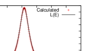
Figure 6.1: The calculated energy-derivative of the phase-shift, $\delta_{p_{3/2}}$(E). For the fitting purpose, the pure Breit-Wigner distribution, $L(E)=\frac{\Gamma_{0}/2}{\Gamma_{0}^{2}/4+(E_{0}-E)^{2}}$ is assumed.

By calculating and fitting the phase-shift according to the formalism in Appendix D, we obtain the resonant energy and width as $E_{0}=308$ keV and $\Gamma_{0}=41$ keV, respectively. These values are obtained using the fitting function as the pure Breit-Wigner distribution:

$$\frac{d\delta_{lj}(E)}{dE}\equiv\frac{\Gamma_{0}/2}{\Gamma_{0}^{2}/4+(E_{0}-E)^{2}},$$ (6.29)

for $l=1$ and $j=3/2$, based on the two-body scattering formalism. The calculated result and its fit are presented in Fig. 6.1.

On the other hand, we can calculate the resonant energy and width by another method, namely by the time-dependent method. With this method, we first have to prepare the initial state for the $1p$-emission. For this purpose, we adopt the “confining potential” method. That is, we assume the modified Hamiltonian,

$$h_{(p_{3/2})}^{conf}=\frac{\bm{p}^{2}}{2\mu}+V_{(p_{3/2})}^{conf}(r),$$ (6.30)

with the confining potential for the $(p_{3/2})$-channel as

$$V_{(p_{3/2})}^{conf}(r)=\left\{\begin{array}[]{cc}V_{(p_{3/2})}(r)&(r\leq R_{b}),\\ V_{(p_{3/2})}(R_{b})&(r>R_{b}),\end{array}\right.$$ (6.31)

with $R_{b}=8.2$ fm. The original and confining potentials are shown in Fig. 6.2(b). The initial state, $\Phi(t=0;\bm{r},\bm{s})$, is defined as an eigen-state of this modified Hamiltonian, namely,

$$h_{(p_{3/2})}^{conf}\ket{\Phi(0)}=E^{conf}\ket{\Phi(0)}.$$ (6.32)

On the other hand, we also consider the eigen-states of the original Hamiltonian as

$$h_{(p_{3/2})}\ket{E_{N}}=E_{N}\ket{E_{N}},$$ (6.33)

with the discretized continuum energies, $\{E_{N}\}$. In order to discretize the continuum, we assume the radial box of $R_{\rm box}=120$ fm in this case, and impose a boundary condition that the wave function satisfies $U_{(p_{3/2})}(r=R_{\rm box})=0$. The energy cutoff is employed as $E_{\rm cut}=40$ MeV. As a result, we have $N_{\rm max}=47$ bases.

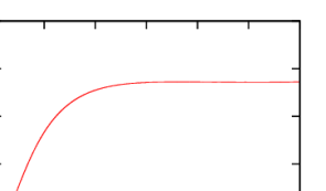
(a) (b)

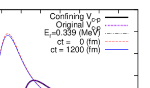
Figure 6.2: (Left panel) The calculated decay width within the confining potential, Eq.(6.31). (Right panel) The original and confining core-proton potentials given by Eqs.(6.26) and (6.31). The Q-value, $E_{0}=0.339$ MeV, and the density distributions at $ct=0$ and $1200$ fm are also shown.

By diagonalizing the $47\times 47$ matrix, $\{\Braket{E_{M}}{h_{(p_{3/2})}^{conf}}{E_{N}}\}$, the initial state can be represented as the expansion on the original eigen-states. That is,

$$\ket{\Phi(0)}=\sum_{N}F_{N}(0)\ket{E_{N}}.$$ (6.34)

This equation has an identical form to Eq.(6.1). Thus, by performing the calculations according to Eqs.(6.3), (6.7) and (6.12), we can determine the Q-value, $E_{0}=\sum_{N}E_{N}\left|F_{N}(0)\right|^{2}$ and the decay width, $\Gamma(t)$. We obtain $E_{0}=339$ keV. The calculated decay width is shown in Figure 6.2(a). After a sufficient time-evolution, the decay width well converges to a constant value, corresponding to the exponential decay-rule. We have obtained $\Gamma_{0}=37$ keV at $ct=1200$ fm, when the decay width is sufficiently converged. These results are consistent to those obtained by calculating the two-body scattering phase-shift, justifying the time-dependent approach. Furthermore, in Figure 6.2, we also show the density distribution, $\left|U_{(p_{3/2})}(r)\right|^{2}$ at $ct=0$ and $1200$ fm. Although these two functions have almost the same form, the later one shows a larger amplitude outside the potential barrier. This indicates the penetration of the valence proton. Consequently, we can observe the time-development of the emitted particle(s) based on this method. This will be a great advantage providing an intuitive view of the decay process, when we will apply this method to the two-proton emissions, in order to discuss the effect of the diproton correlation.

Chapter 7 Two-Proton Emission of ⁶Be

We now apply the time-dependent method to the ground state of ⁶Be nucleus, assuming the three-body structure of $\alpha$+p+p. Because the $\alpha$-particle can be well assumed as a rigid core, this system provides a good testing ground for our method. We also note that, as shown in Figure 7.1, this is one of the closest systems to a true 2p-emitter: the experimental Q-value of the 2p-emission is $1.37$ MeV [55, 52, 179], which is lower than the one-proton resonance energy in ⁵Li, being about $2$ MeV with a broad width [52, 179]. Thus, the sequential process via $\alpha+p$ subsystem is considered to be suppressed, and the two protons should penetrate the potential barrier simultaneously . In this simultaneous 2p-emission, the association between the dinucleon correlations and the 2p-emissions, might be clarified.

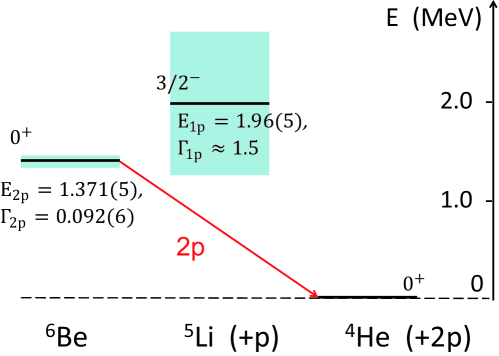
Figure 7.1: The experimental level scheme of ⁶Be and its isotones. The values for ⁵Li are quoted from refs.[52, 218], whereas those for ⁶Be are quoted from refs.[52, 179]. The color-box of each level indicates its decay width.

7.1 Set up for Calculations

Our three-body model consists of $\alpha$-particle as a structureless core (daughter) nucleus and two valence protons. We employ the V-coordinates similarly to Chapters 3 and 4. That is,

$$H_{\rm 3b} = h_{1}+h_{2}+\frac{\bm{p}_{1}\cdot\bm{p}_{2}}{A_{\rm c}m}+v_{\rm p-p}(\bm{r}_{1},\bm{r}_{2}),$$ (7.1)

$$h_{i} = \frac{\bm{p}_{i}^{2}}{2\mu}+V_{\rm c-p}(r_{i})\;\;\;\;(i=1,2),$$ (7.2)

where $h_{i}$ is the single particle (s.p.) Hamiltonian for the relative motion between the core and the $i$-th proton. We assume that the $\alpha$-p potential is spherical, and independent of the spin variables. We also assume that the $\alpha$-particle always remains in the ground state with the spin-parity of $0^{+}$. Thus, similarly in Chapter 4, we need uncorrelated bases only for the $0^{+}$ configuration since the ground state of ⁶Be also has the spin-parity of $0^{+}$. That is,

$$\tilde{\Psi}_{ab}(\xi_{1},\xi_{2}) \longrightarrow \tilde{\Psi}^{(0^{+})}_{n_{a}n_{b}lj}(\xi_{1},\xi_{2})$$ (7.3)

$$=\frac{1}{\sqrt{2(1+\delta_{n_{a},n_{b}})}}\sum_{m}\mathcal{C}^{0,0}_{j,m;j,-m}$$

$$\phantom{000}\left[\phi_{n_{a}ljm}(\xi_{1})\phi_{n_{b}lj-m}(\xi_{2})+\phi_{n_{a}ljm}(\xi_{2})\phi_{n_{b}lj-m}(\xi_{1})\right].$$

In the following, for simplicity, we use simplified labels for the uncorrelated bases: $\ket{\tilde{\Psi}_{K}}$ where $K=\left\{n_{a},n_{b},l,j\right\}$. Then, the time-dependent three-body state, except for the center of mass motion of the whole system, can be expanded as

$$\ket{\Phi(t)}=\sum_{K}C_{K}(t)\ket{\tilde{\Psi}_{K}},$$ (7.4)

where the coefficients $C_{K}(t)$ are given by Eqs. 6.5 and 6.6. All our calculations presented below are performed in the truncated space defined by the energy-cutoff: $\epsilon_{a}+\epsilon_{b}\leq E_{\rm cut}=40$ MeV. We have confirmed that our conclusions do not change even if we employ a larger value of $E_{\rm cut}$.

For the angular momentum channels, we include from $(s_{1/2})^{2}$ to $(h_{11/2})^{2}$ partial waves, similarly to Chapter 4. In order to take into account the effect of the Pauli principle, we exclude the bound $(s_{1/2}$ state from $\phi_{nljm}$ in Eq.(7.3), that is occupied by the protons in the core nucleus. The continuum states are discretized within the radial box of $R_{\rm box}=80$ fm. Even though this model space might be not sufficient to fully describe the 2p-emission of ⁶Be, increasing $l_{\rm max}$ or $R_{\rm box}$ causes a serious rise of computational costs, which makes our calculations practically impossible. Also note that $R_{\rm box}$ limits the interval for time-evolution, because the wave functions are inevitably reflected once it reaches at $r=R_{\rm box}$. This reflection as an calculational artifact causes the deviation from reality at the late-time region. A typical maximum time in our time-dependent calculations is $ct_{\rm max}\sim 2000$ fm, corresponding to the earlier stage of 2p-emissions.

7.1.1 Interactions

We describe the interaction between $\alpha$ and a valence proton using the nuclear Woods-Saxon potential and the Coulomb potential, similarly in the previous Chapters. That is,

$$V_{\rm c-p}(r_{i})=V_{\rm c-p,Nucl.}(r_{i})+V_{\rm c-p,Coul.}(r_{i}),$$ (7.5)

where the nuclear and Coulomb terms are

$$V_{\rm c-N,Nucl.}(r) = \left[V_{0}+V_{ls}r_{0}^{2}(\bm{\ell}\cdot\bm{s})\frac{1}{r}\frac{d}{dr}\right]f(r),$$ (7.6)

$$f(r) = \frac{1}{1+\exp\left(\frac{r-R_{\rm core}}{a_{\rm core}}\right)},$$ (7.7)

and

$$V_{\rm c-p,Coul.}(r)=\left\{\begin{array}[]{cc}\frac{Z_{\rm c}e^{2}}{4\pi\epsilon_{0}}\frac{1}{r}&(r>R_{\rm core}),\\ \frac{Z_{\rm c}e^{2}}{4\pi\epsilon_{0}}\frac{1}{2R_{\rm core}}\left(3-\frac{r^{2}}{R_{\rm core}^{2}}\right)&(r\leq R_{\rm core}).\end{array}\right.$$ (7.8)

For the Coulomb term, we adopt the one of a uniform-charged sphere with the charge radius of the $\alpha$-particle, $R_{\rm core}=r_{c}=1.68$ fm. For the Woods-Saxon part, we use $R_{\rm core}=r_{c}$ and $a_{0}$ = 0.615 fm, whereas strength parameters are fixed as $V_{0}=-58.7$ MeV and $V_{ls}=46.3$ ${\rm MeV(fm)^{2}}$. These parameters reproduce the measured resonance energy and width for the $(p_{3/2})$-channel of $\alpha$-p scattering [179]: it yields $E_{r}(p_{3/2})=1.96$ MeV and $\Gamma_{r}(p_{3/2})=1.56$ MeV. We calculate and fit the derivative of the phase-shift, according to Eq.(D.27), to get this result. We note that this resonance is quite broad and there are large ambiguities in the observed decay width [52, 191, 179, 218], as summarized in Table 1.

$V_{\rm c-p}(r)$ and $V_{\rm c-p}^{conf}(r)$

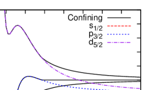
Figure 7.2: The original and confining potentials for $(s_{1/2})$, $(p_{3/2})$ and $(d_{5/2})$ channels in the $\alpha$-p subsystem. The border radius for modifying the potential is 5.7 fm for all the channels.

			$E_{r}$ (MeV)	$\Gamma_{r}$ (MeV)
	This work		1.960000	1.5600
	Ref.[52, 218]		1.96(5)0	$\simeq$ 1.5
	Ref.[191]		2.90(20)	1.0(2)
	Ref.[179]		1.690000	1.0600

Table 1: The resonant energy and width of the ⁵Li nucleus in the $(p_{3/2})$-channel.

For the proton-proton interaction, we use the Minnesota potential, in which the Coulomb term is explicitly included.

$$v_{\rm p-p}(r_{12})=v_{0}e^{-b_{0}r^{2}_{12}}-v_{1}e^{-b_{1}r^{2}_{12}}+\alpha\hbar c\frac{e^{2}}{r_{12}}.$$ (7.9)

For $b_{0},b_{1}$ and $v_{1}$ in Eq.(7.9), we use the same parameters introduced in the original paper [154]. On the other hand, the strength of the repulsive core, $v_{0}$, is adjusted so as to reproduce the empirical Q-value for two protons, $Q_{2p}=1.37$ MeV [52, 179].

7.2 Initial State

As mentioned in Chapter 6, the initial configuration of the two protons is characterized such that the density distribution is localized around the core nucleus and has almost no amplitude outside the core-proton potential barrier. In order to generate such state, we employ the confining potential method [219, 220, 221]. The confining potential for the initial 2p-state is defined as follows. Because the $\alpha$-p subsystem has a resonance at $E_{0}=1.96$ MeV in the $(p_{3/2})$-channel, the two protons in ⁶Be are expected to have a large component for the $(p_{3/2})^{2}$ configuration. Thus, we first modify the core-proton potential for the $(p_{3/2})$-channel at $t=0$ in order to generate a quasi-bound state as follows:

$$V_{{\rm c-p},~{}(p_{3/2})}^{conf}(r)=\left\{\begin{array}[]{cc}V_{{\rm c-p},~{}(p_{3/2})}(r)&(r\leq R_{b}),\\ V_{{\rm c-p},~{}(p_{3/2})}(R_{b})&(r>R_{b}),\end{array}\right.$$

with $R_{b}=5.7$ fm. For the other s.p. channels, we define the confining potential as

$$V_{\rm c-p}^{conf}(r)=\left\{\begin{array}[]{cc}V_{\rm c-p}(r)\phantom{0000}&(r\leq R_{b}),\\ V_{\rm c-p}(r)+V_{b}(r)&(r>R_{b}),\end{array}\right.$$

where $V_{b}(r)=V_{{\rm c-p},~{}(p_{3/2})}(R_{b})-V_{{\rm c-p},~{}(p_{3/2})}(r)$. The original and confining potentials for the $(s_{1/2})$, $(p_{3/2})$ and $(d_{5/2})$ channels are shown in Fig. 7.2. We note that, for this system, the core-proton barrier is mainly due to the centrifugal potential in the $(p_{3/2})$ channel, rather than the Coulomb potential. This situation is quite different from heavy 2p-emitters with a large proton-number, such as ⁴⁵Fe.

⁶Be (g.s.), $t=0$, “full”

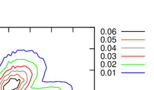
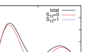
Figure 7.3: The left panel: The 2p-density distribution at $t=0$ for the ground state of ⁶Be. It is obtained by including all the partial waves up to $(h_{11/2})^{2}$, and is plotted as a function of $r_{\rm c-pp}=(r_{1}^{2}+r_{2}^{2}+2r_{1}r_{2}\cos\theta_{12})^{1/2}/2$ and $r_{\rm p-p}=(r_{1}^{2}+r_{2}^{2}-2r_{1}r_{2}\cos\theta_{12})^{1/2}$. The right panel: The corresponding angular distribution obtained by integrating $\bar{\rho}_{2p}$ over $r_{1}$ and $r_{2}$.

⁶Be (g.s.), $t=0$, “$(l=odd)^{2}$ only”

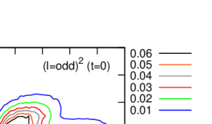
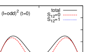
Figure 7.4: The same as Fig. 7.3 but for the case with only the partial waves of $(l=odd)^{2}$.

The initial state for the 2p-emission is solved by diagonalizing the modified Hamiltonian including $V^{conf}_{\rm c-p}(r)$. In Fig. 7.3, we display the density distribution of the initial state obtained in this way.

$$\bar{\rho}_{2p}(t=0;r_{1},r_{2},\theta_{12})=8\pi^{2}r_{1}^{2}r_{2}^{2}\sin\theta_{12}\left|\Phi(t=0;r_{1},r_{2},\theta_{12})\right|.$$ (7.10)

In the left panel of Fig. 7.3, $\bar{\rho}_{2p}$ is plotted as a function of the distance between the core and the center of mass of two protons: $r_{\rm c-pp}=\sqrt{r_{1}^{2}+r_{2}^{2}+2r_{1}r_{2}\cos\theta_{12}}/2$, and the relative distance between two protons: $r_{\rm pp}=\sqrt{r_{1}^{2}+r_{2}^{2}-2r_{1}r_{2}\cos\theta_{12}}$. In the right panel of Fig. 7.3, we also show the angular distributions obtained by integrating $\bar{\rho}_{2p}$ for $r_{1}$ and $r_{2}$.

It is clearly seen that the wave function is confined inside the potential barrier at $r\cong 4$ fm (see Fig. 7.2 again). Furthermore, the 2p-density is concentrated near $r_{\rm p-p}=2$ fm, corresponding to the diproton correlation in the bound nuclei. The corresponding angular distribution becomes asymmetric and has the higher peak at the opening angle $\theta_{12}\cong\pi/6$. This peak is almost due to the spin-singlet configuration, being analogous to the dinucleon correlation.

As we discussed in Chapter 4, the parity-mixing in the subsystem of the core and a nucleon plays an essential role in generating the dinucleon correlation. In order to confirm the similar effect in the 2p-emission, we have performed the same calculations but only with $(p,f,h)^{2}=(l=odd)^{2}$ partial waves. In this case, pairing correlations are partially taken into account only among the s.p. states with the same parity, although the parity-mixing in the core-nucleon subsystem is perfectly ignored. In Fig. 7.4, we show the initial configuration obtained only with $(l=odd)^{2}$ partial waves. In the left panel of Fig. 7.4, there are two comparable peaks at $r_{\rm p-p}=2$ and $5$ fm whereas, in the right panel, the corresponding angular distribution has a symmetric form. This result is in contrast with that in the full mixing case (see Fig. 7.3), where the parity-mixing is fully taken into account (“full mixing”).

The empirical Q-value for the 2p-emission is 1.37 MeV for ⁶Be [52, 179]. However, the original parameters of the Minnesota potential overestimates this value, for instance, by about 50% in the full mixing case. We therefore modify the parameter $v_{0}$ in Eq.(7.9) so as to yield Q = 1.37 MeV. Note that we use the modified $v_{0}$ not only at $t=0$ but also during the time-evolutions.

		6Be, $t=0$				6He
		full	$(l=odd)^{2}$ only	$(p_{3/2})^{2}$ only		full
$\Braket{H_{\rm 3b}}$ (MeV)		1.37	1.37	1.37		$-0.975$
$\Braket{r_{\rm N-N}}$ (fm)		4.92	5.29	5.16		4.67
$\Braket{r_{\rm c-NN}}$ (fm)		3.43	2.64	2.58		3.18
$\Braket{\theta_{12}}$ (deg)		75.9	90.0	90.0		78.0
$(p_{3/2})^{2}$ (%)		88.9	97.1	100.		92.7
$(p_{1/2})^{2}$ (%)		03.1	02.8	000.		01.6
$(s_{1/2})^{2}$ (%)		02.2	00.0	000.		01.3
others,$(l=even)^{2}$ (%)		05.2	00.0	000.		04.2
others,$(l=odd)^{2}$ (%)		00.6	00.1	000.		00.2
$P(S_{12}=0)$ (%)		82.2	80.6	66.6		78.1
$v_{0}$ (MeV)		156.0	88.98	66.69		212.2

Table 2: Calculated properties for the initial state of ⁶Be and ⁶He. The results with all the uncorrelated basis from $(s_{1/2})^{2}$ to $(h_{11/2})^{2}$ are labeled by “full”. Those obtained only with the $(l=odd)^{2}$ and $(p_{3/2})^{2}$ bases are also shown. The values of $v_{0}$ (the strength of the repulsive part) for the nucleon-nucleon interaction (Eq.(7.9)) are tabulated in the last row. The original value is $v_{0}=200.$ MeV [154].

In Table 2, properties of the initial state are summarized. In this Table, for comparison, we also perform the same calculation but in the 3rd case, namely only with the $(p_{3/2})^{2}$ partial wave. The values of $v_{0}$ in the Minnesota potential are tabulated in the last row in Table 2. It is clearly seen that, in the full mixing case, the main component is $(p_{3/2})^{2}$, reflecting that the $(p_{3/2})$ channel has a resonance in the $\alpha$-p subsystem. The mixing of different partial waves are due to the off-diagonal matrix elements of $H_{\rm 3b}$, corresponding to the pairing correlations. The spin-singlet configuration is remarkably enhanced for the full mixing case compared to that in the $(p_{3/2})^{2}$ case. On the other hand, in the case only with $(l=odd)^{2}$, a comparable enhancement of the $S_{12}=0$ configuration exists, even though there is no localization of the two protons as shown in Fig. 7.4. Notice also that in the $(l=odd)^{2}$ case, we have to assume a stronger pairing attraction in order to reproduce the empirical Q-value, as compared to the full-mixing case.

7.2.1 Comparison with ⁶He

From the point of view of the isobaric symmetry in nuclei, it is interesting to compare the initial state of ⁶Be with the ground state of its mirror nucleus, ⁶He. Assuming the $\alpha$+n+n structure, we perform the similar calculation but for the ground state of ⁶He. For the $\alpha$-n system, there is an observed resonance of $(p_{3/2})$ at $E_{r}=0.735(20)$ MeV with its width, $\Gamma_{r}=0.600(20)$ [153, 52]. In order to reproduce this resonance, we exclude the Coulomb term from Eq.(7.5) and modify the depth parameter to $V_{0}=-61.25$ MeV in Woods-Saxon potential. The pairing interaction is adjusted to reproduce $\Braket{H_{\rm 3b}}=-S_{\rm 2n}=-0.975$ MeV [153], yielding $v_{0}=212.2$ MeV in Eq.(4.33). One may concern the difference of $v_{0}$ between ⁶Be and ⁶He. This might be due to an ambiguity in $V_{\rm c-p}$ for ⁶Be originated from a broad resonance in the core-proton subsystem. Improving $V_{\rm c-p}$ in ⁶Be can lead to the more consistent set of parameters among $V_{\rm c-N}$ and $v_{\rm N-N}$. We note that this ambiguity does not affect our qualitative discussions.

⁶He (g.s.), “full”

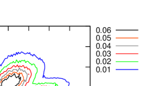
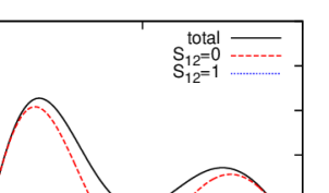
Figure 7.5: The density distribution of the valence two neutrons, $\bar{\rho}_{2n}$, in the ground state of ⁶He. Those are plotted in the same manner as in the left and right panels of Figure 7.3. The partial waves up to $(h_{11/2})^{2}$ are included.

In Fig. 7.5, the two-neutron density distribution is shown in the same manner as in Fig. 7.3. The energetic and structural properties are tabulated in the last column of Table 2. Obviously, the two-neutron wave function in ⁶He has a similar distribution to the 2p-wave function in ⁶Be. Because the two neutrons are bound in this system, the spatial distribution is less expanded in ⁶He. This is why both $\Braket{r_{\rm N-N}}$ and $\Braket{r_{\rm c-NN}}$ have smaller values than those of ⁶Be. The dinucleon correlation is present also in ⁶He, characterized as the spatial localization with the enhanced spin-singlet component [27]. Consequently, the confining potential which we employ provides the initial state of ⁶Be, which can be interpreted as the isobaric analogue state of ⁶He.

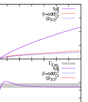
Figure 7.6: The decay probabilities and the decay widths for the 2p-emissions from ⁶Be, obtained with the time-dependent method. The result with all the partial waves in the model-space (full mixing) is plotted by the solid line. For c$t\geq 1000$ (fm), the decay width well converges to a constant value of $88.2$ keV in the full-mixing case. The experimental value, $\Gamma_{\rm Exp}=92\pm 6$ keV [179], is marked by the bold line. The results obtained only with $(p_{3/2})^{2}$ (dotted line) and $(l=odd)^{2}$ (broken line) partial waves are also shown, where the calculated decay widths are clearly underestimated.

7.3 Decay Width

Starting from the initial state obtained in the previous section, we perform the time-evolving calculations for the first $0^{+}$ resonance of ⁶Be. We show the results of the decay-component $N_{d}(t)$ and width $\Gamma(t)$ (see the Eqs.(6.10) and (6.12) in the previous Chapter) obtained with the time-evolution in Fig. 7.6.

In Fig. 7.6, the calculation is carried out up to $ct=0-1400$ fm. We have confirmed that the artifact due to the reflection at $r=R_{\rm box}$ is negligible in this time-interval. One can clearly see that, after a sufficient time-evolution, the decay width converges to a constant value for all the cases, and the exponential decay-rule is realized. Furthermore, the result for the full case yields the saturated value of $\Gamma(t)\cong 88.2$keV, which reproduces the experimental decay width, $\Gamma=92\pm 6$ keV [52, 179]. On the other hand, the limitation of the partial waves only to $(l=odd)^{2}$ or $(p_{3/2})^{2}$ significantly underestimates the decay width. This is caused by an increase of the pairing attraction: With the $(l=odd)^{2}$ or $(p_{3/2})^{2}$ waves only, to reproduce the empirical Q-value, we needed a stronger pairing attraction (see Table 2). The two protons are then strongly bound to each other and are difficult to go outside, even they have a similar energy release of that in the full mixing case.

From these studies, we can conclude that the parity-mixing in the core-proton subsystem is indispensable in order to reproduce simultaneously the Q-value and the decay width of the 2p-emission. This result supports the assumption of the diproton correlation at $t=0$.

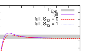
(a) full (b) $(l=odd)^{2}$ only

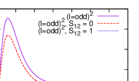
Figure 7.7: (a) The total and the partial decay widths for the spin-singlet and triplet configurations of ⁶Be. The partial waves from $(s_{1/2})^{2}$ to $(h_{11/2})^{2}$ are fully included. (b) The same as panel (a) but for the case with only $(l=odd)^{2}$ partial waves.

For the cases of full mixing and only $(l=odd)^{2}$ partial waves, we also calculate the partial decay widths for the spin-singlet and triplet configurations. The corresponding formula to Eq.(6.16) is given as

$$\Gamma_{S_{12}}(t)\equiv\frac{\hbar}{1-N_{d}(t)}\frac{d}{dt}N_{d,S_{12}}(t),$$ (7.11)

where

$$N_{d,S_{12}}(t) \equiv \Braket{\Phi_{d,S_{12}}(t)}{\Phi_{d,S_{12}}(t)}$$ (7.12)

$$= \int_{0}^{R_{\rm box}}dr_{1}\int_{0}^{R_{\rm box}}dr_{2}\int_{0}^{\pi}d\theta_{12}8\pi^{2}r_{1}^{2}r_{2}^{2}\sin\theta_{12}\left|\Phi_{d,S_{12}}(t;r_{1},r_{2},\theta_{12})\right|^{2},$$

$$\ket{\Phi_{d}(t)} \equiv \ket{\Phi(t)}-\beta(t)\ket{\Phi(0)},$$ (7.13)

with $\beta(t)=\Braket{\Phi(0)}{\Phi(t)}$. The results are shown in Fig. 7.7. Clearly, the spin-singlet configuration almost exhausts the decay width in the full mixing case shown in Fig. 7.7(a). This suggests that the emitted two protons from the ground state of ⁶Be have mostly the configuration of $S_{12}=0$, like a diproton. On the other hand, from Fig. 7.7(b), one can see that the spin-triplet configuration occupies a considerable amount of the total decay width when we exclude $(s,d,g)^{2}$ partial waves.

		full	$(l=odd)^{2}$ only	$(l=odd)^{2}\oplus(s_{1/2})^{2}$	no pairing	exp.data
					($ct=3000$ fm)	[52, 179]
	$\Gamma_{\rm total}$ (keV)	88.2	12.5	35.8	348.	92(6)
	$\Gamma_{S_{12}=0}$ (keV)	87.1	10.7	34.3	232.	-
	$\Gamma_{S_{12}=1}$ (keV)	01.1	01.8	01.5	116.	-

Table 3: The contributions from the spin-singlet and triplet configurations to the decay width of ⁶Be. The values are evaluated at $ct=1200$ fm, except for the “no pairing” case, whose values are evaluated at $ct=3000$ fm. Note that in the all cases, the Q-value of the 2p-emission is reproduced consistently to the experimental value, $1.37$ MeV [52, 179].

In the 2nd and the 3rd columns of Table 3, we tabulate the total and partial widths in the full and the $(l=odd)^{2}$ cases, respectively. The values are estimated at $ct=1200$ fm, where the total widths sufficiently converge. Clearly, there is a significant increase of the spin-singlet width in the full mixing case, by about one-order magnitude larger than that in the case of $(l=odd)^{2}$. On the other hand, we get similar values of the spin-triplet width in the full and $(l=odd)^{2}$ cases. From this result, we can conclude that the core-nucleon parity-mixing is responsible for the enhancement of the spin-singlet emission, although the dominance of the spin-singlet configuration in the initial state is apparent in both the two cases (see Table 2).

The dominance of the spin-singlet configuration is due to the $(s_{1/2})^{2}$ channel. Considering the coupled orbit, $L_{12}\equiv l_{1}\oplus l_{2}$, from the coupling rule to the spin-parity of $0^{+}$, the $(s_{1/2})^{2}$ channel leads to $S_{12}=L_{12}=0$ with $l_{1}=l_{2}=0$. Because there is no centrifugal barrier in this channel, the spin-singlet emission can be dominant. On the other hand, for the spin-triplet configuration, the only $L_{12}=1$ are permitted in order to have the total angular momentum $0^{+}$. Thus, there is a centrifugal barrier for all the channels in the spin-triplet configuration. Consequently, apart from the reduction due to the stronger pairing attraction, the spin-triplet width has similar values to each other in the full-mixing and $(l=odd)^{2}$ cases.

$(l=odd)^{2}\oplus(s_{1/2})^{2}$

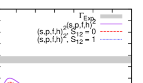
Figure 7.8: The same as Fig. 7.7 but for the $(l=odd)^{2}$ plus $(s_{1/2})^{2}$ case.

In order to check this effect of the $(s_{1/2})^{2}$ waves directly, we perform the same calculation but including the uncorrelated bases with $(l=odd)^{2}$ and $(s_{1/2})^{2}$ configurations. Namely, we add only the $(s_{1/2})^{2}$ waves to the $(l=odd)^{2}$ case. In this case, we use the same parameters for the calculation as those for the full-mixing and the $(l=odd)^{2}$ cases, except for the $v_{0}$ in the Minnesota potential: we use $v_{0}=99.14$ MeV in order to reproduce the Q-value, $Q_{2p}=1.37$ MeV for ⁶Be. The result is shown in Figure 7.8 and in the 4th column in Table 3 in the same manner as the former two cases. One can see that the spin-singlet width is significantly increased due to the existence of the $(s_{1/2})^{2}$ channel, whereas the spin-triplet width has a similar value to those in the full-mixing and $(l=odd)^{2}$ cases. This result supports our former speculation about the role of the $(s_{1/2})^{2}$ channel in the 2p-emission. Notice also that, because of the stronger pairing attraction, the total width in Figure 7.8 is still underestimated than the experimental data.

7.4 Time-Evolution of Decay State

In order to discuss the emission process, we show the density distribution of the decay state,

$$\bar{\rho}_{d}(t)=8\pi^{2}r_{1}^{2}r_{2}^{2}\sin\theta_{12}\rho_{d}(t),$$ (7.14)

$$\rho_{d}(t)=\left|\Phi_{d}(t;r_{1},r_{2},\theta_{12})\right|^{2}.$$ (7.15)

The most of the amplitude of the decay state exists outside the potential barrier, because we prepare the initial state, which is orthogonal to the decay state, so as to have no amplitude in that region. For the presentation, we renormalize the $\bar{\rho}_{d}(t)$ so that its integration become unity at each time:

$$\bar{\rho}_{d}(t)\longrightarrow\frac{\bar{\rho}_{d}(t)}{N_{d}(t)},$$ (7.16)

where $N_{d}(t)$ is the decay probability given by Eq.(6.10). We adopt three sets of radial coordinates in the following. (i) The first set includes $r_{\rm c-pp}=(r_{1}^{2}+r_{2}^{2}+2r_{1}r_{2}\cos\theta_{12})^{1/2}/2$ and $r_{\rm p-p}=(r_{1}^{2}+r_{2}^{2}-2r_{1}r_{2}\cos\theta_{12})^{1/2}$, similarly to the left panel of Figure 7.3. (ii) In the second set, we integrate $\bar{\rho}_{d}$ with respect to the opening angle, $\theta_{12}$, and plot it as a function of $r_{1}$ and $r_{2}$. In order to see the peak-structure clearly, we omit the radial weight $r_{1}^{2}r_{2}^{2}$ in $\bar{\rho}_{d}$ in the second setting. (iii) Within the third set, on the other hand, we integrate $\bar{\rho}_{d}(t)$ over radial distances, and plot it as a function of $\theta_{12}$.

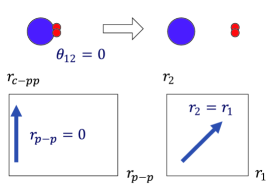
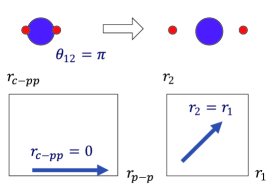
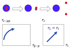
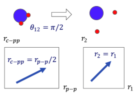
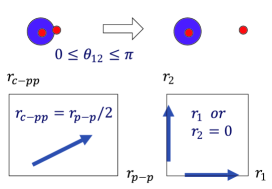
(a) diproton (c) simultaneous, $\theta_{12}=0$ (e) correlated (b) simultaneous, $\theta_{12}=\pi/2$ (d) one-proton (f) sequential

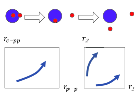
Figure 7.9: Schematic illustrations for the trajectories of different 2p-emission modes.

Before we show the results of the actual calculations, we schematically illustrate the dynamic of the 2p-emissions in Fig. 7.9. From the geometry, one can distinguish two modes: “simultaneous two-proton” and “one-proton ($1p-$)” emissions. The diproton emission is a special case in the first category. The second category corresponds to the case where only one proton penetrate the barrier. The trajectories of three simultaneous 2p- and a $1p$-emissions are schematically shown in Fig. 7.9(a), (b), (c) and (d).

In the simultaneous emissions, two protons are emitted simultaneously with their opening angle remaining from $\theta_{12}=0$ to $\pi$, where $\theta_{12}=0$ corresponds to the diproton emission. Fig. 7.9(a), (b) and (c) correspond to $\theta_{12}=0,\pi/2$ and $\pi$. respectively. In these cases, the density in the $(r_{1},r_{2})$-plane shows the same patterns in these figures, and is concentrated along $r_{1}\cong r_{2}$. The simultaneous emissions with different opening angles can be distinguished only in the $(r_{\rm p-p},r_{\rm c-pp})$-plane: for instance, in the diproton emission, the probability shows mainly along the line with $r_{\rm c-pp}\gg r_{\rm p-p}$, while it is along the line with $r_{\rm c-pp}=0$ for $\theta_{12}=\pi$. In the one-proton emission shown in Fig.7.9(d), only one of the two protons goes through while the other proton remains inside the core nucleus. This is seen as the increment along $r_{\rm c-pp}\cong r_{\rm p-p}/2$ and $r_{1}$ or $r_{2}\cong 0$ lines.

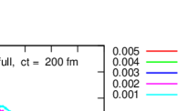
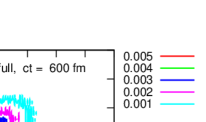
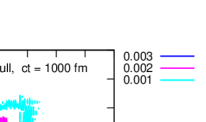
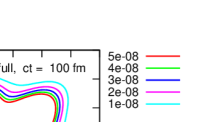
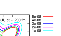
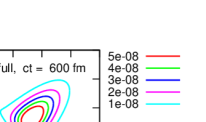
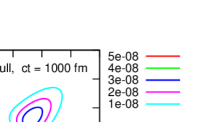
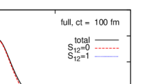
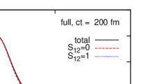
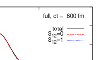
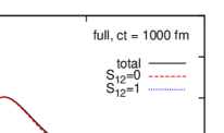
Figure 7.10: The 2p-density distribution for the decay states, $\bar{\rho}_{d}(t)$, obtained with the time-evolving calculations. All the uncorrelated partial waves up to $(h_{11/2})^{2}$ are included. (The left column): These distributions are plotted as a function of $r_{\rm c-pp}=(r_{1}^{2}+r_{2}^{2}+2r_{1}r_{2}\cos\theta_{12})^{1/2}/2$ and $r_{\rm p-p}=(r_{1}^{2}+r_{2}^{2}-2r_{1}r_{2}\cos\theta_{12})^{1/2}$. (The middle column): The same as the left column but as a function of $r_{1}$ and $r_{2}$, obtained by integrating $\bar{\rho}_{d}$ for $\theta_{12}$. In order to clarify the peak(s), the radial weight $r_{1}^{2}r_{2}^{2}$ is omitted. (The right column): The angular distributions of the decay state plotted as a function of the opening angle $\theta_{12}$ between the two protons. It is obtained by integrating $\bar{\rho}_{d}(t)$ for the radial coordinates. Beside the total distribution, the spin-singlet and triplet components are also plotted.

In Fig. 7.9(e) and (f), we additionally illustrate the two hybrid processes. The first one is a “correlated emission”, shown in Fig. 7.9(e). In the correlated emission, the two protons are emitted simultaneously to almost the same direction, holding the diproton-like configuration. In this mode, at the earlier stage of tunneling, the density distribution has a larger amplitude in the region with $r_{1}\cong r_{2}$ and small $\theta_{12}$. In the $(r_{\rm p-p},r_{\rm c-pp})$-plane, It corresponds to the increment of the probability in the region of $r_{\rm p-p}\ll r_{\rm c-pp}$. After the barrier penetration, the two protons separate from each other mainly due to the Coulomb repulsion, increasing $r_{\rm p-p}$.

The second hybrid process is a “sequential emission”, which is shown in Fig. 7.9(f). In this mode, there is a large possibility of that one proton is emitted whereas the other proton remains around the core. The density distribution shows high peaks along $r_{1}\gg r_{2}$ and $r_{1}\ll r_{2}$. In the $(r_{\rm p-p},r_{\rm c-pp})$-plane, it corresponds to the increment along the line of $r_{\rm c-pp}\cong r_{\rm p-p}/2$. Being different from the pure one-proton emission, the remaining proton eventually goes through the barrier also when the core-proton subsystem is unbound.

(Figure is hidden in open-print version.)

Figure 7.11: The same as Fig.7.10 but for the case with only $(l=odd)^{2}$ waves. Notice a different scale in the left column from that in Fig.7.10.

7.4.1 Full-Mixing Case

We now show the results of the time-dependent calculations for the 2p-emission of ⁶Be. We first discuss the full-mixing case which is the closest assumption to reality. The density distribution for the decay state along the time-evolution is shown in Fig. 7.10. The left, middle and right columns correspond to the coordinate sets (i), (ii) and (iii), respectively. The 1st to 4th panels in each column show the decay-density at $ct=100,200,600$ and $1000$ fm, respectively. For a presentation purpose, we normalize $\bar{\rho}_{d}$ at any step of time.

In the left and middle columns of Fig. 7.10, it can be seen that the process in this case is likely the correlated emission shown in Fig. 7.9(e). Contributions from the other modes shown in Fig. 7.9 are small. In the middle column of Fig. 7.10, during the time-evolution, there is a significant increment of $\bar{\rho}_{d}$ along the line with $r_{1}\cong r_{2}$. The corresponding peak in the left column is at $r_{\rm p-p}\ll r_{\rm c-pp}\cong 10$ fm, which means a small value of $\theta_{12}$. It should also be noted that, after the barrier penetration, the two protons lose their diproton-like configuration due to the Coulomb repulsion increasing $r_{p-p}$. Thus, for $r_{\rm c-pp}\geq 10$ fm which is a typical position of the potential barrier from the core, the density distribution extends around the $r_{\rm c-pp}\cong r_{\rm p-p}$ region. In this process, the pairing correlation plays an important role to generate the significant diproton-like configuration before the end of the barrier penetration, similarly to the dinucleon correlations.

In the right column of Fig. 7.10, the distributions are also displayed as a function of the opening angle, $\theta_{12}$. We can clearly see that the decay state has a high peak at $\theta_{12}\cong\pi/6$, and thus the emitted two protons should show the opening angles close to this value. However, this result may appear somewhat inconsistent to the experiments, in which the correlation is much weaker in the observed angular distribution of ⁶Be [72, 56] (see Fig. 5.4). A reason for this discrepancy is due to the final-state interactions (FSIs) at the late stage of propagation of the two protons. In the experiments, the observed spectra and the correlation patterns correspond to those at the late-time region, where the two protons have been much influenced by FSIs. On the other hand, in this thesis, we mainly discuss the earlier stage of the 2p-emission with a small value of $R_{\rm box}$. By taking the FSIs into account at the late stage, we expect that we achieve a better agreement between the theoretical and experimental results. For this purpose, however, we would have to expand the model space defined with $R_{\rm box}$ and $l_{\rm max}$, which would severely increase the computational costs.

7.4.2 Case of $(l=odd)^{2}$ Waves

We next discuss the case only with $(l=odd)^{2}$ waves (Fig. 7.11). Even though the experimental $Q_{\rm 2p}$ and $\Gamma_{\rm 2p}$ are not simultaneously represented in this case (see Fig. 7.7), it is still useful to discuss the density distribution in order to know what happens when the pairing correlation between the parity-plus and minus states in the core-proton subsystem is absent. In Fig. 7.11, the decay density shows strong patterns as the sequential emission introduced in Fig. 7.9(f): significant increments occur along the lines with $r_{\rm c-pp}\cong r_{\rm p-p}/2$ and $r_{1}\gg r_{2}$ or $r_{1}\ll r_{2}$. Notice that the contribution from the simultaneous emissions also exists, especially in the earlier time region. As a result, the decay state has widely spread amplitudes as a mixture of these emission modes. However, the simultaneous mode is quite minor compared with the full mixing case. Notice that the character of a true 2p-emitter exists also in this case: the core-proton resonance is located at $1.96$ MeV which is above $Q_{\rm 2p}1.37$ MeV. Even with the strong pairing attraction and the energy condition of the true 2p-emitter, the process hardly becomes the correlated emission when the parity-mixing is forbidden or extensively suppressed. On the other hand, the angular distribution shows exactly the symmetry form, and is almost invariant during the time-evolution. In this calculation, we exclude the pairing correlation between the parity-plus and minus states in the core-proton, not only at $t=0$ but also during the time-evolution. In other words, there are almost no FSIs to alter the shape of the angular distribution.

7.4.3 Without Pairing Correlation

For a comparison with the above two cases, we also perform similar calculations but by completely neglecting the pairing correlation. In this case, we only consider the uncorrelated Hamiltonian, $h_{1}+h_{2}$. Because of the absence of the non-diagonal components in the Hamiltonian matrix, it can be proved that, if the s.p. resonance is at an energy $\epsilon_{0}$ with its width $\gamma_{0}$, the 2p-resonance should be at $2\epsilon_{0}$ with its width $2\gamma_{0}$ since there are no couplings between the two protons. The 2p-wave function is expanded on the uncorrelated basis with a single set of angular quantum numbers. Namely,

$$\ket{\Phi_{(lj)}(t)}=\sum_{n_{a},n_{b}}C_{n_{a},n_{b},l,j}\ket{\tilde{\Psi}_{n_{a},n_{b},l,j}},$$ (7.17)

where $(lj)=(p_{3/2})$ for ⁶Be. In order to reproduce the empirical Q-value of ⁶Be, we inevitably modify the core-proton potential. We employ $V_{0}=-68.65$ MeV instead of that in the full mixing case to yield the s.p. resonance at $\epsilon_{0}(p_{3/2})=1.37/2=0.685$ MeV, with which the core-proton scattering data are not reproduced and the character of a true 2p-emitter disappears. With this potential, we get the s.p. resonance with a broad width: $\gamma_{0}(p_{3/2})\cong 170$ keV.

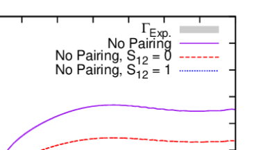
Figure 7.12: The same as Fig. 7.7 but for the case without the pairing correlations.

The result for the 2p-decay width is shown in Fig. 7.12 and in the last column of Table 3. To get the saturated result, we somewhat need a relatively longer time-evolution than that in the full mixing and the $(l=odd)^{2}$ cases. Thus, in Table 3, we estimate the decay at $ct3000$ fm by width the result well converges in this case. We also expand the radial box to $R_{\rm box}=200$ fm in order to neglect the artifact due to the reflection in the longer time-evolution. After a sufficient time-evolution, the total decay width, $\Gamma(t)$, converges to about $340$ keV which is consistent to that expected from the s.p. resonance, $\gamma_{0}(p_{3/2})$. During the time-interval shown in Fig. 7.12, there still remain some oscillations in $\Gamma(t)$. This is a characteristic behavior of the broad resonance, namely the oscillatory deviation from the exponential decay-rule. For the spin-singlet and triplet configurations, their contributions have exactly the ratio of $2:1$. This result is simply due to including only $(p_{3/2})^{2}$ partial waves, and is proved by calculating the coefficient $D_{J}$ in Eq.(3.82).

(Figure is hidden in open-print version.)

Figure 7.13: The same as Fig. 7.10 but for the case without the pairing correlations and a deeper $V_{\rm c-p}$.

By comparing the results with those in the full mixing case, where the pairing correlations are fully taken into account, we can clearly see a decisive role of the pairing correlations in 2p-emissions. Assuming the empirical Q-value, if we explicitly consider the pairing correlations, the decay width becomes narrow and agrees with the experimental data. On the other hand, in the no pairing case, we need a modified core-proton interaction to reproduce the empirical Q-value, and the core-proton resonance properties become inconsistent with the experimental data. Even though the Q-value is adjusted in this way, the calculated 2p-decay width is significantly overestimated in this case. Namely, we cannot simultaneously reproduce the experimental Q-value and the decay width with the no pairing assumption. If one is focused to reproduce them simultaneously, one may need unphysical assumptions for the core-proton interactions. In the next Section, we will present further investigations about this problem.

In Fig. 7.13, we show the density distribution of the decay state during the time-evolution. Obviously, the process is the sequential or, moreover, like the one-proton emission in this case. There is a significant increase of the density along the lines with $r_{\rm c-pp}\cong r_{\rm p-p}/2$ and, consistently, with $r_{1}\gg r_{2}$ and $r_{1}\ll r_{2}$ (see Fig. 7.9 again). On the other hand, the probability for the simultaneous and correlated emissions are negligibly small. We emphasize that this is quite different from that in the full mixing case, where the correlated emission is apparent. Notice that, with a disagreement with the experimental decay width, this result should not correspond to the 2p-emission of ⁶Be in reality. This situation can be interpreted as the limit where the core-proton resonance plays an excessively dominant role.

7.5 Role of Pairing Correlation

In order to discuss the role of the pairing correlations in the 2p-emission, we calculate the 2p-decay width for different Q-values, for the full-mixing and the no pairing cases.

To this end, the Q-value is varied by modifying the parameter $V_{0}$ in the core-proton potential (Eq.(7.6)). In the previous calculations, we used $V_{0}=-58.7$ and $V_{0}=-68.65$ MeV in the full mixing and the no pairing cases, respectively. These original values yield the empirical Q-value, $Q_{\rm 2p}=1.37$ MeV. In addition to these original values, we change the value of $V_{0}$ as $V_{0}\pm 0.5$ and $V_{0}\pm 1.0$ MeV. The calculated decay widths are well converged after a sufficient time-evolution in all the cases. We note that, in the full mixing case, we adopt the same pairing interaction as in the previous calculation.

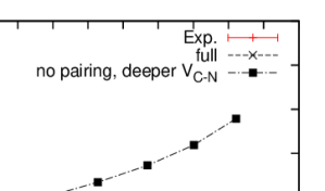
Figure 7.14: The calculated decay widths for the 2p-emission of ⁶Be, as a function of the Q-value. The Q-value is varied by modifying the core-proton potential. The experimental values are indicated as the point at $Q_{\rm 2p}=1.37$ and $\Gamma_{\rm 2p}=0.092(6)$ MeV.

In Fig. 7.14, the decay width is plotted as a function of the Q-value. The decay width in each case is evaluated at $ct=1200$ and $3000$ fm in the full mixing and the no pairing cases, respectively. Clearly, the no pairing calculation overestimates the decay width, in all the region of $Q_{\rm 2p}$. Namely, the three-body system becomes easier to decay without the pairing correlations compared to the full-mixing case, even if we consider the same value of the total energy (Q-value). In other words, the pairing correlation plays an essential role in the meta-stable state, stabilizing it against particle emissions. Moreover, as we have confirmed in the previous section, the emission modes with and without the pairing correlations are essentially different to each other: the correlated emission is suggested if the pairing correlation is fully considered, whereas omitting it yields the sequential emission. Of course, this result can be associated with the character of ⁶Be as a true 2p-emitter. Consequently, we conclude that the pairing correlation must be treated explicitly in the meta-stable states, or one would miss the essential effect on the dynamical phenomena.

7.6 Summary of this Chapter

We have applied the time-dependent three-body model to ⁶Be, which has a close character to the true 2p-emitter. The initial state of ⁶Be has the diproton correlation, similarly to the dineutron correlation in the ground state of ⁶He. The empirical relation between $Q_{\rm 2p}$ and $\Gamma_{\rm 2p}$ is well reproduced by fully including the pairing correlation (in the full mixing case). We have also showed that the decay process at its earlier stage is mainly the correlated emission, in which the two protons are emitted to the same direction with $S_{12}=0$, like a diproton. The dominance of the spin-singlet decay width is explained as the effect of the $(s{1/2})^{2}$ wave.

We have performed the calculations by switching off a part of the pairing correlation in order to study its role in the 2p-emissions. First, we excluded the parity-mixing in the core-proton subsystem, equivalently to forbidding the diproton correlation in particle-bound nuclei. Notice that the character of a true 2p-emitter exists also in this assumption. In this case, the decay width and its spin-singlet ratio are remarkably underestimated compared to the full mixing case. The decay process has a large component of the sequential emission, which is quite different from the correlated emission. From this result, we can infer that the diproton correlation is essential in describing the 2p-emission. Second, we completely omitted the pairing correlation, and adjusted the mean-field between the core and a proton to reproduce the Q-value of the emitted two protons. The character of a true 2p-emitter no longer exists in this case. It was shown that the pairing correlation plays an essential role in the meta-stable states: omitting the pairing correlation leads to a largely overestimated decay width, and almost the perfect sequential emission which scarcely exists in the full mixing case.

At this moment, the dependence of 2p-emissions on the initial diproton correlation is strongly suggested, but this has not yet been proved. Indeed, the FSIs must be taken into account at the late stage of the time-evolution, in order to probe the diproton correlation with the experimental observables. Towards this goal, we plan to expand our model space defined with $R_{\rm box}$ and $l_{\rm max}$, enabling us to perform the longer time-evolution where the FSIs play a dominant role. The sensitivity to the diproton correlation is translated to the initial-configuration dependence of observables. If the $Q_{\rm 2p}$ and $\Gamma_{\rm 2p}$ are by no means reproduced simultaneously by excluding the diproton correlation at $t=0$, we will be able to conclude the presence of the diproton correlation. Possibly, for instance, we will also infer that the observed signals associated with the diproton-emission [72, 56] reflect the survived components originally emerged at $t=0$. The time-dependent method, which can distinguish the cause and the effect in the observables, will be a powerful tool in these discussions. We also mention that the other approaches within complex-energy framework is hard to separately discuss the early and late time regions, or equivalently, the cause and the effect. Therefore, our studies will produce a complementary point of view to the 2p-emission and possibly the diproton correlation.

The expansion of the model space, however, will lead to a serious increment of computational costs. To overcome this difficulty, we will have to adopt an improved boundary condition which does not emerge the reflection of the wave function at the edge of the radial box, or/and more efficient bases which can reduce the dimension of the Hamiltonian matrix. Additionally, we should also concern the pairing interaction. The pairing interaction employed in this thesis should be regarded as an effective interaction, since it is inconsistent to the scattering problem of 2pin vacuum due to our modification of $v_{0}$. Within further expanded model space, it may cause the unphysical result. One may also introduce a three-body force, which works only if three particles are close to each other [222, 33, 35]. The effect of this three-body force on decay processes is an important topic, in regard to whether such an interaction is really just a phenomenological one or has a physical meaning beyond the two-body force.

Chapter 8 Two-Proton Emission of ¹⁶Ne

For further investigation of 2p-emissions in this Chapter, we take up another 2p-emitter, ¹⁶Ne. To this end, we assume the three-body system of ¹⁴O and two valence protons. The quantum meta-stability is treated within the time-dependent framework. In the case of ⁶Be discussed in the previous Chapter, our time-dependent three-body model well reproduced the experimental $Q_{\rm 2p}$ and $\Gamma_{2p}$ simultaneously. It suggests that the three-body assumption is valid for this nucleus. On the other hand, it has been a serious problem that a similar theoretical three-body model within the complex-energy framework do not simultaneously reproduce the $Q_{\rm 2p}$ and $\Gamma_{2p}$ of other light 2p-emitters [171]. Thus, it is worthwhile to check whether our model works or not for these nuclei. The application to the ¹⁶Ne nucleus to be discussed in this Chapter is one example of studies towards this direction.

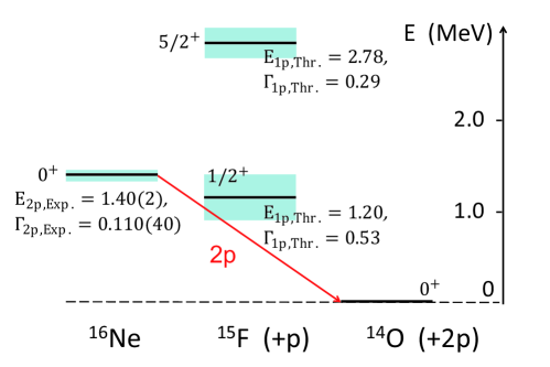
Figure 8.1: The level scheme of ¹⁶Ne and its isotones. The printed values for ¹⁶Ne are taken from the Ref. [60]. Those for ¹⁵F are calculated with the core-proton interaction which is originally introduced in the Ref. [193]. The color-box of each level indicates its decay width.

In Figure 8.1, we show the level scheme of ¹⁶Ne and its daughter nuclei after the $1p$- and 2p-emissions, measured from the ground state of ¹⁴O. Indeed, the $1p$-resonance of the ¹⁴O+p in the $(s_{1/2})$-channel is located near the 2p-resonance of ¹⁶Ne. Its width, $\Gamma_{\rm 1p}\simeq 500$ keV is so large that one may wonder whether the resonance character truly exists in this system or not. The sequential emission through the core-proton channel is expected to be minor, due to its broad width. We also stress that there are still ambiguities in the experimental data of the first resonance of ¹⁵F [58, 192, 193, 223, 224, 225, 226]. Consequently, it is still unclear whether the ¹⁶Ne nucleus is a true 2p-emitter or not. In this work, we will assume a relatively low energy and narrow width in the $(s_{1/2})$-channel, as detailed in the next section.

8.1 Set up for Calculations

General assumptions for the numerical calculations are similar to those for the ⁶Be in the previous Chapter. We assume that the core nucleus, ¹⁴O is a structureless particle with the spin-parity of $0^{+}$. Because the first resonance state of ¹⁶Ne also has the spin-parity of $0^{+}$, we only need the $0^{+}$ uncorrelated basis for the valence two protons. The calculations are performed in the truncated space defined by the energy-cutoff: $\epsilon_{a}+\epsilon_{b}\leq E_{\rm cut}=40$ MeV. The continuum states are discretized within a radial box of $R_{\rm box}=80$ fm. For the angular momentum channels, we take $l_{\rm max}=5$, that is, we include all the partial waves from $(s_{1/2})^{2}$ to $(h_{11/2})^{2}$.

$V_{\rm c-p}(r)$ and $V_{\rm c-p}^{conf}(r)$

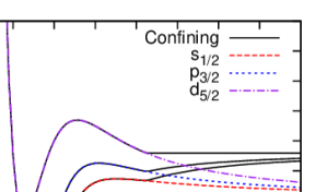
Figure 8.2: The original and confining potentials for the $(s_{1/2})$, $(p_{3/2})$ and $(d_{5/2})$ channels in the ¹⁴O-p subsystem. The border radius for modifying the potential is 8.5 fm for all the channels.

¹⁶Ne (g.s.), $t=0$, “full”

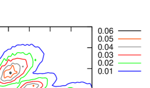
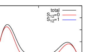
Figure 8.3: (The left panel) The 2p-density distribution at $t=0$ for the ground state of ¹⁶Ne. It is obtained by including all the partial waves up to $(h_{11/2})^{2}$, and plotted as a function of $r_{\rm c-pp}=(r_{1}^{2}+r_{2}^{2}+2r_{1}r_{2}\cos\theta_{12})^{1/2}/2$ and $r_{\rm p-p}=(r_{1}^{2}+r_{2}^{2}-2r_{1}r_{2}\cos\theta_{12})^{1/2}$. (The right panel) The angular distribution at $t=0$ obtained by integrating $\bar{\rho}_{2p}(t=0)$ with $r_{1}$ and $r_{2}$.

We assume the Woods-Saxon and Coulomb potentials between the core and a proton, similarly to Eq.(7.5). We employ the same parameters as those in the Ref. [193], in which the authors discussed the scattering problem of ¹⁴O+p theoretically. The first and second resonances obtained with these parameters are shown in Fig. 8.1. We calculate and fit the derivative of the phase-shift, according to Eq.(D.27), to get $E_{\rm 1p}$ and $\Gamma_{\rm 1p}$. These values are consistent to several experimental results [58, 225, 226].

For the proton-proton pairing interaction, we use the Minnesota potential given by Eq.(4.33) in this case. In order to reproduce the Q-value of 2p-emission, $Q_{\rm 2p}\equiv\Braket{H_{\rm 3b}}=1.40$ MeV, we adjust the strength of the repulsive part as $v_{0}=126.2$ MeV. The other parameters in the Minnesota potential are fixed to the original values in ref.[154].

The initial 2p-state for the time-evolution is defined as a quasi-bound state obtained with the confining potentials, similarly to the previous calculations for ⁶Be. The confining potentials for ¹⁶Ne are defined as follows. In Chapter 4, we have confirmed that in ^17,18Ne nuclei, the valence two protons are mainly in the $(d_{5/2})^{2}$-orbit. Because ¹⁶Ne is an isotope of these nuclei, the first resonance of ¹⁶Ne is also expected to have a large component of $(d_{5/2})^{2}$-configuration. According to this consideration, for the single particle (s.p.) $(d_{5/2})$-channel, we modify the core-proton potential at $t=0$ in order to fix the quasi-bound state as follows.

$$V_{{\rm c-p},~{}(d_{5/2})}^{conf}(r)=\left\{\begin{array}[]{cc}V_{{\rm c-p},~{}(d_{5/2})}(r)&(r\leq R_{b}),\\ V_{{\rm c-p},~{}(d_{5/2})}(R_{b})&(r>R_{b}),\end{array}\right.$$ (8.1)

with $R_{b}=8.5$ fm in this case. For other s.p. channels, we define it as

$$V_{\rm c-p}^{conf}(r)=\left\{\begin{array}[]{cc}V_{\rm c-p}(r)\phantom{0000}&(r\leq R_{b}),\\ V_{\rm c-p}(r)+V_{b}(r)&(r>R_{b}),\end{array}\right.$$ (8.2)

where $V_{b}(r)=V_{{\rm c-p},~{}(d_{5/2})}(R_{b})-V_{{\rm c-p},~{}(d_{5/2})}(r)$. The original and confining potentials for the $(s_{1/2})$, $(p_{3/2})$ and $(d_{5/2})$ channels are shown in Fig. 8.2.

By diagonalizing the modified Hamiltonian including $V_{\rm c-p}^{conf}(r)$, we obtain the initial 2p-state. In Figure 8.3, we show the initial density, $\rho_{2p}(t=0)$, and its angular distribution. One can clearly see a significant diproton correlation, characterized by the localization of the two protons in the $S_{12}=0$ configuration. The spin-singlet ratio is obtained as $P(S_{12}=0)=87.9$%. The prominent three peaks are due to the dominant $(d_{5/2})^{2}$ wave, with its probability of $49.56$% in this state. In addition, the $(s_{1/2})^{2}$ wave has a comparable probability of $44.70$% in this state. The other waves with $(l=odd)^{2}$ and $(l=even)^{2}$ carry the probabilities of $3.61$% and $2.13$%, respectively. It is worthwhile to compare this result with that of ¹⁷Ne obtained in Chapter 4. By comparing the left panel of Fig. 8.3 with Fig. 4.10(a), it can be seen that the spatial distribution is a little more extended in the ¹⁶Ne nucleus. This is consistent with the increment of the $(s_{1/2})^{2}$ wave, which has a long tail outside the core-proton potential. While this result can be interpreted as a characteristic difference between the bound and meta-stable 2p-states, anyway, the diproton correlation is still suggested in the initial state of ¹⁶Ne. If our time-dependent calculation yields the decay width that is consistent with the experiments, we can associate the behavior of the emitted two protons (at the earlier stage) with the diproton correlation.

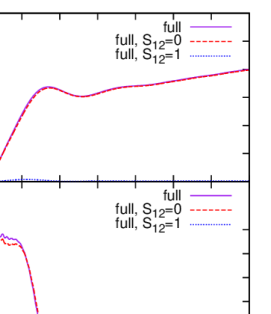
Figure 8.4: The decay probabilities and the decay width of 2p-emissions from ¹⁶Ne, obtained with the time-dependent method. Those for the spin-singlet and triplet configurations are also plotted. In calculations, all the partial waves up to $(h_{11/2})^{2}$ are included. The parameters of the pairing interaction are adjusted to reproduce the experimental Q-value, $Q_{\rm 2p,Exp.}=1.40(2)$ MeV [60]. Note that the experimental decay width, $\Gamma_{\rm 2p,Exp.}=110\pm 40$ keV [60] is too higher to be indicated in the lower panel.

8.2 Decay Width

The results for the decay probability and the decay width are shown in Fig. 8.4. The calculation is carried out up to $ct=2800$ fm where the reflection at $R_{\rm box}$ can be neglected. Unfortunately, there is a large discrepancy between the calculated and the experimental decay widths. In Fig. 8.4, after a sufficient time-evolution, the calculated decay width approximately converges to $\Gamma_{\rm 2p,Thr.}\simeq 2-3$ keV, which is underestimated against the experimental value, $\Gamma_{\rm 2p,Exp.}=110\pm 40$ keV [60]. This discrepancy would not be attributed to our small model space, or the uncertainties in the time-dependent calculation since a similar three-body model calculation also yielded a similar discrepancy [171, 47]. Additionally, in the earlier time region, the decay probability shows a big bump, causing a large oscillation in the decay width, $\Gamma(t)$. We do not know exactly whether this bump is just an artifact, or originates from the initial configuration, including the diproton correlation.

In order to investigate a possible cause of the underestimated decay width, we carry out similar calculations but with different values of $v_{0}$ in the Minnesota pairing interaction, intuitively discarding the fine set up for the Q-value. In Fig. 8.5, we show the results obtained with $v_{0}=200.0,168.0$ and $126.2$ MeV. The first value is identical to the original parameter [154], whereas the third value is that used in Fig. 8.4. The decay width is reproduced if we take $v_{0}=168$ MeV, which yields $Q_{\rm 2p,Thr.}=2.04$ MeV. In this case, compared with the previous case with $Q_{\rm 2p,Thr.}=1.40$, the two protons have a larger energy to overcome the potential barriers, and the decay width becomes also larger, leading to the agreement with the experimental value. It means that our naive three-body model leads to an over stabilization against the 2p-emission of ¹⁶Ne.

Notice also that there remains sizable oscillations in $\Gamma(t)$ even after a sufficient time-evolution. We conjecture that the mixing of the two resonances, namely those in the $(s_{1/2})$ and $(d_{5/2})$-channels of the core-proton subsystem, is responsible for this result. However, we do not explore deeply into this problem here. Indeed, we will rather discuss what causes the over stabilization of the two protons.

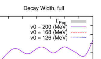
Figure 8.5: The decay widths obtained for different values of $v_{0}$ in the Minnesota pairing attraction. The corresponding Q-values are $Q_{\rm 2p}=2.48$, $2.04$ and $1.40$ MeV for $v_{0}=200$, $168$ and $126.2$ MeV, respectively. The experimental decay width, $\Gamma_{\rm 2p,Exp.}=110\pm 40$ keV [60], is also indicated by the shaded area.

8.3 Possibilities of Improvements

The first possible cause of the over stabilization of ¹⁶Ne is a lack of core excitations in the present theoretical model. In other words, the intrinsic degrees of freedom of the core nucleus may not be neglected for ¹⁶Ne. One may wonder why the present model works well for ⁶Be, but does not for ¹⁶Ne. This is due to the stability of the core nuclei, namely $alpha$-particle and ¹⁴O for ⁶Be and ¹⁶Ne, respectively. The first excited state of $\alpha$ is located at $E=20.2$ MeV, which is much higher than the first excited state of ¹⁴O at $E=5.1$ MeV [153]. Thus, the core excitation may be relatively important in ¹⁶Ne compared to ⁶Be.

Indeed, from recent studies on weakly-bound nuclei, it is expected that excitations of the core nucleus play an important role in the halo structure and the electro-magnetic excitations of these nuclei [227, 228, 229, 230, 231, 232, 233]. For the meta-stable processes, it has been recognized that a coupling of the valence particle with these degrees of freedom might enhance the tunneling probability and thus increase the decay width [80, 234, 235, 236]. The similar effect of the core excitation is expected to exist in the 2p-emission, which might restore an discrepancy between the calculated and the experimental decay widths. The most possible source of these excitations is the deformation of the core nucleus. However, even if the core is not deformed, the considerable component of these excitations exist, namely the “two-particle and two-hole (2p2h-)” type of excitations from the naive shell structure, due to the pairing correlations. It includes the 2p2h-excitations by two protons, two neutrons and a proton-neutron pair. The former two are caused by the ordinary pairing correlations, whereas the last one is associated with the tensor force [231]. Taking these core excitations into account means an extension of the inert-core model, and may lead to a relaxation of over stabilization of 2p-emissions. However, for this purpose, we must expand the model space, which would increase the cost of calculations. To treat it correctly will be a challenging task in our future works.

The second possibility is due to a model-dependence of the pairing interaction, as partially discussed in the previous Chapter. In this thesis, we have adopted the simple Minnesota interaction between two protons. With other interactions, which include the spin-orbit or the momentum-dependence, might reproduce the experimental $Q_{\rm 2p}$ and $\Gamma_{\rm 2p}$ simultaneously. Furthermore, in order to reproduce the total Q-value, we have intuitively modified the parameter of the Minnesota potential in this work. However, by modifying the parameter, two-nucleon scattering property at infinitely far from the core is no longer reproduced. This deviation may affect the calculated results, especially for the meta-stable processes, in which the final-state interactions play an important role even far from the core. To improve this point, we will have to install the density-dependence into the pairing interaction, or employ the phenomenological three-body force, which works only when all the particles are localized in a small region. A work towards this direction is in the progress now.

Chapter 9 Summary of Thesis

We have theoretically investigated the diproton correlation and its effect on the two-proton emission. These are both the exotic features of proton-rich nuclei which are located far from the beta-stability line, and thus are the novel interests in current nuclear physics. Furthermore, these two phenomena can be strongly connected to each other, because they have a common basis of physics, namely the nuclear pairing correlation. The diproton and dineutron correlations are the intrinsic structures characterized by a spatial localization of two nucleons of the same kind with a large component of the spin-singlet configuration. These are exotic features which cannot be reproduced within the pure mean-field theory of nuclei, and are strongly related to the density-dependence of pairing correlations, which is an important prediction from the modern theory for nuclear structures. Recently, the two-proton decays and emissions have attracted much interests as an efficient tool to probe the diproton correlation. In the observables of the emitted two protons, information on the diproton correlation may be reflected. In order to establish this idea, further investigations were still necessary with a realistic assumptions for calculations. Revealing their fundamental relation is expected to provide another way to probe the nuclear pairing phenomena and the dinucleon correlations, simultaneously a development of the advanced nuclear theory which covers both the low and high density-regions, and both bound and meta-stable systems. Nevertheless, few people have discussed this possibility within a realistic assumptions of calculations [49, 145].

For this purpose, we have carried out the quantum three-body model calculations in this thesis. Our calculations provide semi-microscopic descriptions for the nuclear pairing correlations. By performing model calculations and analyzing their results, we have obtained several important conclusions.

In the former half of this thesis, we have discussed the diproton correlation in bound proton-rich nuclei. By calculating ¹⁸Ne, ¹⁸O and ¹⁷Ne nuclei, we have confirmed that the diproton correlation exists in the ground state of these nuclei, similarly to the dineutron correlation in neutron-rich nuclei. In these systems, a prominent localization of the two protons and neutrons are predicted. The spin-singlet configuration takes the major contribution to this localization. It has also been shown that the Coulomb repulsive force between the two protons does not affect significantly this correlation. Even though this repulsion extends the density distribution of two nucleons and weakens the binding energy, its effect is not sufficiently strong to destroy the diproton correlation. Our calculations have indicated that the effect of the Coulomb force reduces the pairing energy gap only by about 10 %, being consistent to other theoretical studies. We have also found that whether the dinucleon correlations exist or not is insensitive to the total binding energy of a three-body systems. Namely, the dinucleon correlations can be considered not only in loosely bound nuclei, but also in deeper bound systems.

From these results, we can conclude that the dinucleon correlations exist almost independently of (i) whether the pair consists of protons or neutrons, and of (ii) whether that the pair is loosely or deeply bound to the core nucleus. Eventually, the dinucleon correlations should be discussed as a common property of both stable and unstable nuclei.

In the latter half of this thesis, we have focused on the relation between the diproton correlation and the two-proton emissions. In two-proton emissions, a pair of protons are emitted directly from the parent nucleus. This process is a typical meta-stable phenomenon governed by the quantum tunneling effect, and can be an promising tool to probe the diproton correlation. It can be expected that if the valence two protons have the diproton correlation inside the potential barrier, its effect can be reflected in the decay observables. However, in order to extract information on the diproton correlation from the decay observables, one has to treat both the quantum meta-stability and the many-body property on an equal footing.

For this purpose, we have developed the time-dependent three-body model. In this model, the initial 2p-state is defined as a quasi-bound state within a phenomenological confining potential. The quantum tunneling process can be treated by solving the time-dependent Schrödinger equation. The sensitivity of 2p-emissions to the diproton correlation has been discussed by studying its dependence on the initial configuration of the two protons, with or without a diproton-like clustering. We would like to emphasize that our time-dependent approach has an advantage to treat the quantum meta-stable processes, enabling us to distinguish the essential cause of phenomena. Especially, for two-proton emissions, several theoretical works have already been done, most of which have been based on the time-independent formalism. However, the relation between the observables in the 2p-emissions and the nuclear intrinsic structures, including the diproton correlation, has not been discussed. Thus, our present study provides a novel insight into these important problems.

By applying this model to the ⁶Be nucleus, which is the simplest two-proton emitter, We have obtained several results suggesting that the diproton correlation is reflected in the decay observables. To be more specific, first, we have confirmed that the experimental two-proton decay-width of 6Be is well reproduced only by assuming the diproton correlation in the initial state. Furthermore, the decay width is mostly from the spin-singlet configuration. Second, the emitted two protons are expected to have a diproton-like cluster at the early stage of emissions, due to the pairing correlations (that is, the correlated emission). We have also performed the same calculations but based on the pure mean-field model, completely ignoring the pairing correlations. In such calculations, the decay width is severely overestimated, and the emission process shows mostly the pure sequential emission, differing from the case with the pairing correlations. These results suggest the importance of the diproton correlation in the 2p-emissions.

At this moment, the strong dependence of the 2p-emission on the diproton correlation is suggested. It means that the 2p-emission can be an effective tool to evince the diproton correlation. In order to prove it completely, however, there still remain several open problems listed below.

1. Final-state interactions: Our present results have predicted a significant correlated emission, including the diproton-like clustering in the early stage of the two-proton emissions of ⁶Be. However, on the other hand, there is no significant signal of the correlated emission in the experimental angular and energy correlation patterns. A reason for this discrepancy may be the final-state interactions (FSIs). In the experimental data, there is a strong modification of the correlation pattern by the FSIs among all the particles. Especially, the long-ranged Coulomb forces can extensively affect the two protons during their propagation. Consequently, the observed data correspond to the late stage of the emission process. It has yet to be clarified how the diproton correlation at the initial and the earlier stages are reflected in the experiments. In order to address this question, by taking the FSIs sufficiently into account, we would need to expand our model-space so that a longer time-evolution can be carried out. However, at the same time, it inevitably leads to a serious increment of computing costs, and one would need to develop more economic procedures for the three-body model calculations to resolve this problem. Such procedures include, e.g. assuming a sophisticated boundary condition to avoid the reflection of wave functions at the edge of the box, and employing an efficient bases to reduce the dimension of the Hamiltonian matrix.

2. Pairing interaction in the asymptotic region: In the present study, we have used the nuclear potential between two nucleons, by modifying its parameter to reproduce the total Q-value of the 2p-emissions. However, such modified potential is not consistent to the two-nucleon scattering property in vacuum, and may lead to a serious error in the calculated results. Especially, in order to reproduce the angular distributions of the two protons, we might have to weaken the pairing attraction in the asymptotic region. For this purpose, one should install the density-dependence into the pairing potential, or employ a three-body force which works as a short-ranged attraction between three particles. The effect of the three-body force on the two-nucleon emissions and decays is an important problem, as well as whether such an three-body force has an physical meaning or not.

3. Core excitations: For the ⁶Be nucleus, our three-body model well reproduces the experimental data of the Q-value and decay-width. However, for another light two-proton emitter, ¹⁶Ne, our calculations have not been successful in reproducing them consistently: the 2p-decay width is considerably underestimated even if we employ the appropriate parameters for the total Q-value. We note that this problem is not only in our calculations but also in other studies based on a similar three-body model to ours [171, 47]. Given this discrepancy, we anticipate a limitation of the simple three-body model assuming an inert, structure-less core, and the importance of the core excitations. Similar problems have been reported in other studies of, e.g. the nuclear meta-stable processes [80, 160, 234, 235, 236] and the structures of nuclei far from the beta-stability line [227, 228, 229, 230, 231, 232, 233], suggesting that the core excitation plays an important role in these phenomena. To discard the assumption of an inert core may resolve the discrepancy between the calculated and the observed 2p-widths. Treating it correctly will be an important task in our future works. We also note that the explicit treatment of the core excitations would be connected to the role of the tensor force, because the tensor force causes the 2p2h-type of excitations of the core [231].

After these improvements, our time-dependent method will be more sophisticated and will be able to reveal the essential relation between the diproton correlation and the two-proton emissions. Moreover, similar time-dependent approaches can be applied to describe other quantum meta-stable processes in few-body systems. Especially, considering the dinucleon correlations, the most important one may be the two-neutron ($2n$-) emissions. In analogy to the relation between the diproton correlation and the 2p-emissions, the $2n$-emissions can be a powerful tool to examine the dineutron correlation in neutron-rich nuclei. Because of the absence the long-ranged Coulomb FSIs, a theoretical treatment may be easier than that for the 2p-emissions, although the problems of an asymptotic pairing interaction and of the core excitations still remain. Work towards this direction is also an challenging task in the future.

The quantum meta-stability plays an important role in various situations in our world. Especially, those of three or more fermions, or with many degrees of freedom, have been one of the most important subjects in modern physics. However, in spite of its importance, there remain a lot of unknown aspects of the quantum meta-stability. The theoretical treatment still needs a further development, where the two complementary (or competing) frameworks coexist at present. Atomic nuclei, which show various radioactive processes, are one of the most suitable fields to discuss these physics. The knowledge gained in this field can be extended to other quantum meta-stable phenomena with many fermions or with strong correlations. Understanding the quantum meta-stability among different scales will be a great benchmark in future physics.

Appendix A Numerov Method

This is the numerical method to solve an ordinary differential equation in which only the zeroth and the second order terms are included, such as

$$\left[\frac{d^{2}}{dx^{2}}+f(x)\right]U(x)=0,$$ (A.1)

where $f(x)$ is an arbitrary source function. The solution, $U(x)$, is sampled at equidistant points $x_{n},(n=0\sim N)$ where the distance between two sampling points is defined as $a$. With this method, starting from the solution values at two consecutive sampling points, namely $U_{0}\equiv U(x_{0})$ and $U_{1}\equiv U(x_{1})$, we can calculate the remaining solution values as

$$U_{n+2}=\frac{(2-5a^{2}f_{n+1}/6)U_{n+1}-(1+a^{2}f_{n})U_{n}}{1+a^{2}f_{n+2}/12}+\mathcal{O}(a^{6}),$$ (A.2)

where we neglect $\mathcal{O}(a^{6})$. The derivation of Eq.(A.2) is based on the discrete Taylor expansion for $U(x)$ until the fifth order. Considering the two sampling points, $x_{n-1}=x_{n}-a$ and $x_{n+1}=x_{n}+a$, Taylor expansions are given as

$$U_{n+1} \equiv U(x_{n}+a)$$ (A.3)

$$= U_{n}+aU^{\prime}_{n}+\frac{a^{2}}{2!}U^{\prime\prime}_{n}+\frac{a^{3}}{3!}U^{(3)}_{n}+\frac{a^{4}}{4!}U^{(4)}_{n}+\frac{a^{5}}{5!}U^{(5)}_{n}+\mathcal{O}(a^{6}),$$

$$U_{n-1} \equiv U(x_{n}-a)$$ (A.4)

$$= U_{n}-aU^{\prime}_{n}+\frac{a^{2}}{2!}U^{\prime\prime}_{n}-\frac{a^{3}}{3!}U^{(3)}_{n}+\frac{a^{4}}{4!}U^{(4)}_{n}-\frac{a^{5}}{5!}U^{(5)}_{n}+\mathcal{O}(a^{6}),$$

where $U^{(m)}_{n}\equiv\left.d^{m}U(x)/dx^{m}\right|_{x=x_{n}}$. The sum of these two equations gives

$$U_{n-1}+U_{n+1}=2U_{n}+a^{2}U^{\prime\prime}_{n}+\frac{a^{4}}{12}U^{(4)}_{n}+\mathcal{O}(a^{6}).$$ (A.5)

Solving this equation for $a^{2}U^{\prime\prime}_{n}$ leads to

$$-a^{2}U^{\prime\prime}_{n}=2U_{n}-U_{n-1}-U_{n+1}+\frac{a^{4}}{12}U^{(4)}_{n}+\mathcal{O}(a^{6}).$$ (A.6)

In this equation, we can replace $U^{\prime\prime}_{n}$ to $-f_{n}U_{n}$ because of Eq.(A.1). Similarly, for the fourth term in the right hand side, we can use

$$U^{(4)}(x)=\frac{d^{2}}{dx^{2}}[-f(x)U(x)].$$ (A.7)

The numerical definition of the second derivative is given as the second order difference quotient, that is

$$\frac{d^{2}}{dx^{2}}[-f(x)U(x)]\Rightarrow-\frac{f_{n-1}U_{n-1}-2f_{n}U_{n}+f_{n+1}U_{n+1}}{a^{2}}.$$ (A.8)

After these replacements, Eq.(A.6) is transformed as

$$a^{2}f_{n}U_{n}=2U_{n}-U_{n-1}-U_{n+1}-\frac{a^{4}}{12}\frac{f_{n-1}U_{n-1}-2f_{n}U_{n}+f_{n+1}U_{n+1}}{a^{2}}+\mathcal{O}(a^{6}).$$ (A.9)

Finally, we solve this equation for $U_{n+1}$ to get

$$U_{n+1}=\frac{(2-5a^{2}f_{n}/6)U_{n}-(1+a^{2}f_{n-1})U_{n-1}}{1+a^{2}f_{n+1}/12}+\mathcal{O}(a^{6}),$$ (A.10)

which is equivalent to Eq.(A.2).

Appendix B Formalism of Many-Body Coordinates

In this Chapter, we introduce the general formalism for the transformation of coordinates of many-particle systems. For $N$ particles in the three dimensional space, one needs $N$ coordinates of space, $\{\bm{x}_{i}\},\;i=1\sim N$. In general, these degrees of freedom are separated into the center-of-mass coordinate, $\bm{r}_{G}$, and $N-1$ relative coordinates, ${\bm{r}_{k}},\;k=1\sim N-1$. The V-coordinate used in this thesis is just one kind of definitions of ${\bm{r}_{k}},\;k=1,2$, and its definition is detail in the following. The derivations of the three-body Hamiltonian in the V-coordinates is also introduced. For more general formulations and applications, see e.g. the textbook [237].

B.1 Coordinates for Many-Body Problems

We start our discussions from the original coordinates $\bm{x}_{i}$ and their conjugate momenta $\bm{\pi}_{i}$. These satisfy

$$[(\bm{x}_{i})_{\mu},(\bm{\pi}_{j})_{\nu}]=i\hbar\delta_{ij}\cdot\delta_{\mu\nu}\;\Longrightarrow\;\bm{\pi}_{i}=-i\hbar\frac{\partial}{\partial\bm{x}_{i}},$$ (B.1)

where $\mu$ and $\nu=x,y,z$. Here we define the column vector $\vec{X}$ and $\vec{\Pi}$, whose $i$-th component is $\bm{x}_{i}$ and $\bm{\pi}_{i}$, respectively.

$$\vec{X}\equiv\left[\begin{array}[]{c}\bm{x}_{1}\\ \vdots\\ \bm{x}_{N}\end{array}\right],\qquad\vec{\Pi}\equiv\left[\begin{array}[]{c}\bm{\pi}_{1}\\ \vdots\\ \bm{x}_{N}\end{array}\right].$$ (B.2)

Using the transform-matrix $U$, one can define the new set of coordinates, $\{\bm{r}_{i}\}$, as follows:

$$\vec{R}\equiv\left[\begin{array}[]{c}\bm{r}_{1}\\ \vdots\\ \bm{r}_{N}\end{array}\right]=U\vec{X}\quad\Longleftrightarrow\quad\vec{X}=U^{-1}\vec{R},$$ (B.3)

or equivalently,

$$\bm{r}_{i}=\sum_{j=1}^{N}U_{ij}\bm{x}_{j}\quad\Longleftrightarrow\quad\bm{x}_{i}=\sum_{j=1}^{N}(U^{-1})_{ij}\bm{r}_{j}.$$ (B.4)

The conjugate momenta are also written by applying the chain-rule:

$$\bm{\pi}_{i}=-i\hbar\frac{\partial}{\partial\bm{x}_{i}}=-i\hbar\sum_{j}\frac{\partial\bm{r}_{j}}{\partial\bm{x}_{i}}\frac{\partial}{\partial\bm{r}_{j}}=\sum_{j}U_{ji}\bm{p}_{j}.$$ (B.5)

Thus, indicating the transverse matrix of $U$ as ${}^{t}U$, the conjugate momenta of $\vec{R}$ can be defined as

$$\vec{P}\equiv\left[\begin{array}[]{c}\bm{p}_{1}\\ \vdots\\ \bm{p}_{N}\end{array}\right]=({}^{t}U)^{-1}\vec{\Pi}\quad\Longleftrightarrow\quad\vec{\Pi}={}^{t}U\vec{P},$$ (B.6)

or equivalently,

$$\bm{p}_{i}=\sum_{j=1}^{N}({}^{t}U)^{-1}_{ij}\bm{\pi}_{j}\quad\Longleftrightarrow\quad\bm{\pi}_{i}=\sum_{j=1}^{N}{}^{t}U_{ij}\bm{p}_{j}.$$ (B.7)

Note that the conjugate relation is still satisfied as

$$[(\bm{r}_{i})_{\mu},(\bm{p}_{j})_{\nu}]=i\hbar\delta_{ij}\cdot\delta_{\mu\nu}.$$ (B.8)

The transform-matrix, $U$, can be chosen arbitrarily and there is no mathematical discrimination between different $U$s. However, in practice, there are two major coordinates used to solve the many-body problems. In this thesis, we choose so called “core-center coordinates” defined by the transform-matrix,

$$U\equiv\left(\begin{array}[]{ccccc cc}1&0&0&\cdots&0&0&-1\\ 0&1&0&\cdots&0&0&-1\\ \vdots&&&&&&\\ 0&0&0&\cdots&0&1&-1\\ \frac{m_{1}}{M}&\frac{m_{2}}{M}&\frac{m_{3}}{M}&\cdots&\frac{m_{N-2}}{M}&\frac{m_{N-1}}{M}&\frac{m_{N}}{M}\end{array}\right),$$ (B.9)

where its inverse matrix is given by

$$U^{-1}\equiv\left(\begin{array}[]{ccccc c}1-\frac{m_{1}}{M}&-\frac{m_{2}}{M}&-\frac{m_{3}}{M}&\cdots&-\frac{m_{N-1}}{M}&1\\ &&&&&\\ -\frac{m_{1}}{M}&1-\frac{m_{2}}{M}&-\frac{m_{3}}{M}&\cdots&-\frac{m_{N-1}}{M}&1\\ &&&&&\\ -\frac{m_{1}}{M}&-\frac{m_{2}}{M}&1-\frac{m_{3}}{M}&\cdots&-\frac{m_{N-1}}{M}&1\\ \vdots&&&&&\\ -\frac{m_{1}}{M}&-\frac{m_{2}}{M}&-\frac{m_{3}}{M}&\cdots&1-\frac{m_{N-1}}{M}&1\\ &&&&&\\ -\frac{m_{1}}{M}&-\frac{m_{2}}{M}&-\frac{m_{3}}{M}&\cdots&-\frac{m_{N-1}}{M}&1\\ \end{array}\right),$$ (B.10)

with $M\equiv\sum_{i=1}^{N}m_{i}$. In these coordinates, the vector $\bm{r}_{N}$ indicates the center-of-mass motion, whereas $\bm{r}_{k}$ with $k=1\sim(N-1)$ indicates the relative motion between the central core and the $k$-th particle. We schematically indicate these coordinates in the case of three-body systems in Figure B.1.

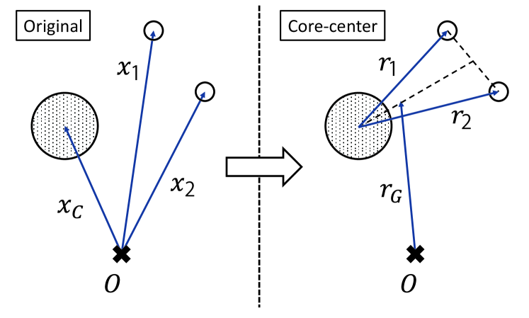
Figure B.1: (left panel) The original coordinates for the three-body system. (right panel) The core-center coordinates.

We briefly introduce another famous coordinates, namely “Jacobi coordinates”. Those are defined by

$$U_{J}\equiv\left(\begin{array}[]{ccccc cc}1&-1&0&0&\cdots&0&0\\ &&&&&&\\ \frac{m_{1}}{m_{12}}&\frac{m_{2}}{m_{12}}&-1&0&\cdots&0&0\\ &&&&&&\\ \frac{m_{1}}{m_{123}}&\frac{m_{2}}{m_{123}}&\frac{m_{23}}{m_{123}}&-1&\cdots&0&0\\ \vdots&&&&&&\\ \frac{m_{1}}{m_{12\cdots(N-1)}}&\frac{m_{2}}{m_{12\cdots(N-1)}}&\cdots&\cdots&\cdots&\frac{m_{N-1}}{m_{12\cdots(N-1)}}&-1\\ &&&&&&\\ \frac{m_{1}}{M}&\frac{m_{2}}{M}&\cdots&\cdots&\cdots&\frac{m_{N-1}}{M}&\frac{m_{N}}{M}\end{array}\right),$$ (B.11)

and its inverse matrix is given by

$$U_{J}^{-1}\equiv\left(\begin{array}[]{ccccc c}\frac{m_{2}}{m_{12}}&\frac{m_{3}}{m_{123}}&\frac{m_{4}}{m_{1234}}&\cdots&\frac{m_{N}}{M}&1\\ &&&&&\\ -\frac{m_{1}}{m_{12}}&\frac{m_{3}}{m_{123}}&\frac{m_{4}}{m_{1234}}&\cdots&\frac{m_{N}}{M}&1\\ &&&&&\\ 0&-\frac{m_{12}}{m_{123}}&\frac{m_{4}}{m_{1234}}&\cdots&\frac{m_{N}}{M}&1\\ &&&&&\\ 0&0&-\frac{m_{123}}{m_{1234}}&\cdots&\frac{m_{N}}{M}&1\\ \vdots&&&&&\\ 0&0&0&\cdots&-\frac{m_{12\cdots(N-1)}}{M}&1\end{array}\right),$$ (B.12)

with $m_{12\;\cdots N^{\prime}}\equiv\sum_{i=1}^{N^{\prime}}m_{i}$. This set of coordinates has been used as well as the core-center coordinates for nuclear few-body models [237]. In this thesis, we use these coordinates only for the two relative momenta in the three-body system, in order to calculate $\Braket{h_{\rm c-NN}}$ and $\Braket{h_{\rm N-N}}$ in Chapters 4 and 7.

B.2 Hamiltonian of Three-Body System

In this thesis, we study the quantum three-body systems consisting of the core-nucleus and the two valence nucleons. We approximately use the same mass for a proton and a neutron. Thus, the masses of the core and a valence nucleon are $m_{C}=A_{C}m$ and $m_{1}=m_{2}=m$, respectively, where $A_{C}$ is the mass-number of the core. The total Hamiltonian written in the original coordinates, $\{\bm{x}_{i}\}$, is given as

$$H = \frac{\bm{\pi}_{1}^{2}}{2m}+\frac{\bm{\pi}_{2}^{2}}{2m}+\frac{\bm{\pi}_{C}^{2}}{2A_{C}m}$$ (B.13)

$$+V_{C-N_{1}}(\bm{x}_{1}-\bm{x}_{C})+V_{C-N_{2}}(\bm{x}_{2}-\bm{x}_{C})+v_{N_{1}-N_{2}}(\bm{x}_{1}-\bm{x}_{2}),$$

where we assigned the third coordinate, ${\bm{x}_{3}}$, to the core-nucleus.

To get the Hamiltonian in the core-center, or sometimes called “V-coordinates” for three-body systems, we consider the transform-matrix, $U$, defined as

$$U=\left(\begin{array}[]{ccc}1&0&-1\\ 0&1&-1\\ \frac{m}{M}&\frac{m}{M}&\frac{A_{C}m}{M}\end{array}\right)\quad\Longleftrightarrow\quad U^{-1}=\left(\begin{array}[]{ccc}1-\frac{m}{M}&-\frac{m}{M}&1\\ -\frac{m}{M}&1-\frac{m}{M}&1\\ -\frac{m}{M}&-\frac{m}{M}&1\end{array}\right),$$ (B.14)

where $M=m_{1}+m_{2}+m_{C}=(A_{C}+2)m$. The transformed coordinates are written as

$$\left[\begin{array}[]{c}\bm{r}_{1}\\ \bm{r}_{2}\\ \bm{r}_{3}\end{array}\right]=U\left[\begin{array}[]{c}\bm{x}_{1}\\ \bm{x}_{2}\\ \bm{x}_{C}\end{array}\right]=\left[\begin{array}[]{c}\bm{x}_{1}-\bm{x}_{C}\\ \bm{x}_{2}-\bm{x}_{C}\\ \frac{m}{M}\bm{x}_{1}+\frac{m}{M}\bm{x}_{2}+\frac{A_{C}m}{M}\bm{x}_{C}\end{array}\right],$$ (B.15)

where $\bm{r}_{3}$ corresponds to the center-of-mass, $\bm{r}_{G}$. Notice also that $\bm{x}_{1}-\bm{x}_{2}=\bm{r}_{1}-\bm{r}_{2}$ and thus we can simply replace $v_{N_{1}-N_{2}}(\bm{x}_{1}-\bm{x}_{2})\longrightarrow v_{N_{1}-N_{2}}(\bm{r}_{1}-\bm{r}_{2})$. On the other hand, the conjugate momenta are transformed as

$$\left[\begin{array}[]{c}\bm{\pi}_{1}\\ \bm{\pi}_{2}\\ \bm{\pi}_{C}\end{array}\right]={}^{t}U\left[\begin{array}[]{c}\bm{p}_{1}\\ \bm{p}_{2}\\ \bm{p}_{G}\end{array}\right]=\left[\begin{array}[]{c}\bm{p}_{1}+\frac{m}{M}\bm{p}_{G}\\ \bm{p}_{2}+\frac{m}{M}\bm{p}_{G}\\ -\bm{p}_{1}-\bm{p}_{2}+\frac{A_{C}m}{M}\bm{p}_{G}\end{array}\right].$$ (B.16)

From Eq.(B.16), the kinetic terms can be re-written as

$$\frac{\bm{\pi}_{1}^{2}}{2m}+\frac{\bm{\pi}_{2}^{2}}{2m}+\frac{\bm{\pi}_{C}^{2}}{2A_{C}m}$$ (B.17)

$$\qquad=\frac{1}{2}\left(\frac{1}{m}+\frac{1}{A_{C}m}\right)\bm{p}_{1}^{2}+\frac{1}{2}\left(\frac{1}{m}+\frac{1}{A_{C}m}\right)\bm{p}_{2}^{2}+\frac{1}{A_{C}m}\bm{p}_{1}\cdot\bm{p}_{2}+\frac{1}{2M}\bm{p}_{G}^{2}$$

$$\qquad=\frac{\bm{p}_{1}^{2}}{2\mu}+\frac{\bm{p}_{2}^{2}}{2\mu}+\frac{\bm{p}_{1}\cdot\bm{p}_{2}}{A_{C}m}+\frac{\bm{p}_{G}^{2}}{2M}$$ (B.18)

where $\mu=m(A_{C}+1)/A_{C}$. As the final result, the total Hamiltonian takes the form below.

$$H = \frac{\bm{p}_{1}^{2}}{2\mu}+\frac{\bm{p}_{2}^{2}}{2\mu}+\frac{\bm{p}_{1}\cdot\bm{p}_{2}}{A_{C}m}+\frac{\bm{p}_{G}^{2}}{2M}$$ (B.19)

$$+V_{C-N_{1}}(\bm{r}_{1})+V_{C-N_{2}}(\bm{r}_{2})+v_{N_{1}N_{2}}(\bm{r}_{1}-\bm{r}_{2}).$$

Notice that in Eq.(B.19), the center-of-mass motion is separated from the three-body relative motion. Assuming that $\bm{p}_{G}=\bm{0}$, the three-body Hamiltonian, $H_{\rm 3b}$, in Chapter 3 is correctly derived.

Appendix C Scattering Problem with Contact Potential

In this Chapter, we discuss the nucleon-nucleon scattering problem with the phenomenological contact potential, $V(\bm{r})=V_{0}\delta(\bm{r})$. The contact potential can provide physical meanings only within the truncated space defined by the energy cutoff, $E_{\rm cut}$. With an arbitrary $E_{\rm cut}$ value, one can determine $V_{0}$ to reproduce the scattering character, namely the scattering length or the phase shift at the lower energy limit. The Schrödinger equation of this scattering problem is written as

$$\left[-\frac{\hbar^{2}}{2\mu}\nabla^{2}_{\bm{r}}+V_{0}\delta(\bm{r})\right]\phi(\bm{r})=E\phi(\bm{r}),$$ (C.1)

with the incident energy $E$. Here $\mu=m/2$ is the relative mass for the two-nucleon system where $m$ is the one-nucleon mass.

We define the relative momentum, $k\equiv\frac{\sqrt{2\mu E}}{\hbar}$, and the converted potential, $v(\bm{r})\equiv\frac{2\mu}{\hbar^{2}}V_{0}\delta(\bm{r})=v_{0}\delta(\bm{r})$. Using these symbols, we can modify the Schrödinger equation as below.

$$\left[\nabla^{2}_{\bm{r}}+k^{2}\right]\phi(\bm{r},k)=v(\bm{r})\phi(\bm{r},k).$$ (C.2)

The outgoing solution of this equation is formally represented with a Green’s function [12]:

$$G^{(+)}(\bm{r},\bm{r}^{\prime},k) \equiv \lim_{\eta\rightarrow 0}\int\frac{d^{3}\bm{p}}{(2\pi)^{3}}\frac{e^{i\bm{p}\cdot(\bm{r}-\bm{r}^{\prime})}}{p^{2}-k^{2}-i\eta}$$ (C.3)

$$= \frac{1}{4\pi}\frac{e^{ik|\bm{r}-\bm{r}^{\prime}|}}{|\bm{r}-\bm{r}^{\prime}|},$$ (C.4)

which satisfies

$$\left[\nabla^{2}_{\bm{r}}+k^{2}\right]G^{(+)}(\bm{r},\bm{r}^{\prime},k) = -\int\frac{d^{3}\bm{p}}{(2\pi)^{3}}e^{i\bm{p}\cdot(\bm{r}-\bm{r}^{\prime})}$$ (C.5)

$$= -\delta({\bf r}-{\bf r}^{\prime}).$$ (C.6)

The scattered wave function within the outgoing boundary condition, $\phi^{(+)}$, is formulated as

$$\phi^{(+)}(\bm{r},k)=\phi^{(+)}_{0}(\bm{r},k)-\int d^{3}\bm{r}^{\prime}G^{(+)}(\bm{r},\bm{r}^{\prime},k)v(\bm{r}^{\prime})\phi^{(+)}(\bm{r}^{\prime},k),$$ (C.7)

where $\phi^{(+)}_{0}(\bm{r},k)$ indicates the outgoing plane-wave. Substituting $v(\bm{r}^{\prime})=v_{0}\delta(\bm{r}^{\prime})$, we can solve the $\phi^{(+)}(\bm{r}^{\prime},k)$ as

$$\phi^{(+)}(\bm{r},k) = \phi^{(+)}_{0}(\bm{r},k)-\int d^{3}\bm{r}^{\prime}G^{(+)}(\bm{r},\bm{r}^{\prime},k)v_{0}\delta(\bm{r}^{\prime})\phi^{(+)}(\bm{r}^{\prime},k),$$ (C.8)

$$= \phi^{(+)}_{0}(\bm{r},k)-G^{(+)}(\bm{r},\bm{0},k)v_{0}\phi^{(+)}(\bm{0},k),$$ (C.9)

$$= \phi^{(+)}_{0}(\bm{r},k)-\frac{v_{0}}{4\pi}\phi^{(+)}(\bm{0},k)\frac{e^{ikr}}{r}.$$ (C.10)

Here we used Eq.(C.4) to get the last formula. Now we can derive the well-known formula for the scattered wave, that is

$$\phi^{(+)}(\bm{r},k)=\phi^{(+)}_{0}(\bm{r},k)+f(k)\frac{e^{ikr}}{r},$$ (C.11)

by defining the “form factor”, $f(k)$, as

$$f(k)=-\frac{v_{0}}{4\pi}\phi^{(+)}(\bm{0},k).$$ (C.12)

It means that the scattered wave was disrupted only at $\bm{r}=\bm{0}$, consistently to the infinitesimal range of the contact interaction.

On the other hand, substituting Eq.(C.3) into Eq.(C.7), we can derive an alternative formula for the scattered wave:

$$\phi^{(+)}(\bm{r},k)=\phi^{(+)}_{0}(\bm{r},k)-v_{0}\phi^{(+)}(\bm{0},k)\lim_{\eta\rightarrow 0}\int\frac{d^{3}\bm{p}}{(2\pi)^{3}}\frac{e^{i\bm{p}\cdot\bm{r}}}{p^{2}-k^{2}-i\eta}.$$ (C.13)

At $\bm{r}=\bm{0}$, assuming the energy cutoff, $E_{C}\longleftrightarrow k_{C}$, we can apparently solve this equation. That is

$$\phi^{(+)}(\bm{0},k) = \phi^{(+)}_{0}(\bm{0},k)-v_{0}\phi^{(+)}(\bm{0},k)\frac{1}{2\pi^{2}}\int_{0}^{k_{C}}dp\frac{p^{2}}{p^{2}-k^{2}}$$ (C.14)

$$= 1-\frac{v_{0}}{2\pi^{2}}\phi^{(+)}(\bm{0},k)\left[k_{C}+\frac{k}{2}\ln\left|\frac{k_{C}-k}{k_{C}+k}\right|\right].$$ (C.15)

Thus we get

$$\phi^{(+)}(\bm{0},k)=\left(1+\frac{v_{0}}{2\pi^{2}}\left[k_{C}+\frac{k}{2}\ln\left|\frac{k_{C}-k}{k_{C}+k}\right|\right]\right)^{-1},$$ (C.16)

which is the complementary equation to Eq.(C.12).

C.1 Low Energy Limit

In the following, we consider the s-wave at the low energy limit ($k\rightarrow 0$). As well known, the form factor can be written as

$$f_{s}(k)=\frac{1}{k}e^{i\delta_{s}}\sin\delta_{s}$$ (C.17)

where $\delta_{s}$ is the phase shift. It leads to an asymptotic formula below:

$$|f_{s}(k)|^{2} = \frac{\sin^{2}\delta_{s}}{k^{2}}=\frac{1}{k^{2}+k^{2}\cot^{2}\delta_{s}}$$ (C.18)

$$\Longrightarrow k\cot\delta_{s} = \left(\frac{1}{|f_{s}(k)|^{2}}-k^{2}\right)^{1/2}\simeq\frac{1}{|f_{s}(k)|}\left(1-\frac{k^{2}|f_{s}(k)|^{2}}{2}\right).$$ (C.19)

From Eqs.(C.12), (C.16) and (C.19), the phase shift of the s-wave can be approximated as

$$k\cot\delta_{s}\simeq-\frac{4\pi}{v_{0}}\left(1+\frac{v_{0}}{2\pi^{2}}\left[k_{C}+\frac{k}{2}\ln\left|\frac{k_{C}-k}{k_{C}+k}\right|\right]\right).$$ (C.20)

Note that the logarithmic term is expanded as a polynomial of $k$:

$$\ln\left|\frac{k-k_{C}}{k+k_{C}}\right|\simeq-2\frac{k}{k_{C}}+\mathcal{O}\left(\left(\frac{k}{k_{C}}\right)^{3}\right),$$ (C.21)

where there are no terms on the order of $k^{0}$. On the other hand, there is an well-known empirical formula for $k\cot\delta_{s}$ at $k\rightarrow 0$, such as

$$k\cot\delta_{s}\simeq-\frac{1}{a_{\rm nn}}+\frac{r_{\rm nn}}{2}k^{2}.$$ (C.22)

Here $a_{\rm nn}$ is the nucleon-nucleon scattering length whose empirical value is $-18.5$ fm, whereas the $r_{\rm nn}$ is the effective range. Comparing the leading terms in Eqs. (C.20) and (C.22), the strength $V_{0}$ can be defined within the energy-cutoff $k_{C}$ to reproduce the scattering length. That is

$$-\frac{4\pi}{v_{0}}\left(1+\frac{v_{0}k_{C}}{2\pi^{2}}\right) = -\frac{1}{a_{\rm nn}}$$

$$\Longrightarrow v_{0} = 4\pi\left(\frac{1}{a_{\rm nn}}-\frac{2}{\pi}k_{C}\right)^{-1}=4\pi\left(\frac{\pi a_{\rm nn}}{\pi-2a_{\rm nn}k_{C}}\right).$$ (C.23)

Remembering $v_{0}/2=\mu V_{0}/\hbar^{2}$, consequently we get the fitting formula for the contact potential:

$$V_{0} = \frac{\hbar^{2}}{2\mu}\left(\frac{4\pi^{2}a_{\rm nn}}{\pi-2a_{\rm nn}k_{C}}\right).$$ (C.24)

It should be noted that Eq. (C.24) is valid at $k\rightarrow 0$ limit. However, in practical cases, the parameter defined with $a_{\rm nn}=-18.5$ fm may be too strong especially for the valence nucleons. Thus the lower value, e.g. $a_{\rm nn}=15.0$ fm, is also used to prepare the appropriate paring attraction as often as the original value. In this thesis, we confirmed that our conclusions do not change even if we employ $a_{\rm nn}=15.0$ fm instead of $a_{\rm nn}=18.5$ fm.

Appendix D Two-Body Scattering with Spherical Potential

Our goal in this Appendix is to derive the fitting formula for the phase-shift of two-body scattering problems. For simplicity, we assume that the potential between two particles is spherical. For quantum resonances in two-body systems, one can usually solve the asymptotic waves analytically. The phase shift and its derivative can be computed by using these asymptotic waves, where it indicates the pole(s) of the S-matrix for the resonance. Even if one is interested in the scattering problem with three or more particles, it is often necessary to solve the partial two-body systems in order to, e.g. prepare the fine two-body interactions.

D.1 Solutions in Asymptotic Region

Assuming the relative wave function as $\phi_{ljm}(\bm{r},\bm{s})=R_{lj}(r)\mathcal{Y}_{ljm}(\bar{\bm{r}},\bm{s})$, the radial equation of this problem reads

$$\left[-\frac{\hbar^{2}}{2\mu}\left\{\frac{d^{2}}{dr^{2}}-\frac{l(l+1)}{r^{2}}\right\}+V_{lj}(r)-E\right]U_{lj}(r,E)=0,$$ (D.1)

where we defined $U_{lj}(r,E)\equiv rR_{lj}(r)$ from the radial wave function. The relative energy, $E$, for the scattering problem satisfies

$$E>\lim_{r\rightarrow\infty}V_{lj}(r)\equiv 0.$$ (D.2)

The equivalent but more convenient radial equation takes the form given by

$$\left[\frac{d^{2}}{d\rho^{2}}-\frac{l(l+1)}{\rho^{2}}-\frac{V_{lj}(r)}{E}+1\right]U_{lj}(\rho)=0,$$ (D.3)

where $\rho\equiv kr$ defined with the relative momentum, $k(E)\equiv\sqrt{2E\mu}/\hbar$. In numerical calculations, this type of equations can be solved with, e.g. Numerov method explained in Chapter 3.

To calculate the phase-shift and also other important quantities, asymptotic solutions of Eq.(D.3) are often necessary. In the following, we note these solutions for two major potentials frequently used in nuclear physics.

D.1.1 Short-Range Potential

Short-range potentials, including nuclear interactions, are characterized as

$$\lim_{r\rightarrow\infty}V_{lj}(r)<\mathcal{O}(r^{-2}).$$ (D.4)

The asymptotic condition can be satisfied at $\rho\gg 1$. A general solution in this region can be written as

$$\frac{U_{lj}(\rho)}{\rho}=C_{1}j_{l}(\rho)+C_{2}n_{l}(\rho),$$ (D.5)

with spherical Bessel and Neumann functions, such as

$$j_{l}(kr) \longrightarrow \frac{1}{kr}\sin\left(kr-l\frac{\pi}{2}\right),$$ (D.6)

$$n_{l}(kr) \longrightarrow \frac{-1}{kr}\cos\left(kr-l\frac{\pi}{2}\right).$$ (D.7)

Or equivalently, the out-going and in-coming waves can be given as

$$h^{(+)}_{l}(kr) \equiv j_{l}(kr)+in_{l}(kr)\longrightarrow\frac{1}{ikr}e^{i\left(kr-l\frac{\pi}{2}\right)},$$ (D.8)

$$h^{(-)}_{l}(kr) \equiv j_{l}(kr)-in_{l}(kr)\longrightarrow\frac{-1}{ikr}e^{-i\left(kr-l\frac{\pi}{2}\right)}.$$ (D.9)

Using the coefficients $A_{lj}$ and $B_{lj}$, a general solution takes the form of

$$\frac{U_{lj}(kr)}{kr} = A_{lj}(E)h^{(+)}_{l}(kr)+B_{lj}(E)h^{(-)}_{l}(kr)$$ (D.10)

$$= B_{lj}(E)[S_{lj}(E)h^{(+)}_{l}(kr)+h^{(-)}_{l}(kr)],$$

with the S-matrix, $S_{lj}(E)\equiv A_{lj}(E)/B_{lj}(E)$. Note that $\left|S_{lj}(E)\right|^{2}=1$ from the conservation law of the flux. Introducing the phase-shift, $\delta_{lj}(E)$ as $S_{lj}(E)\equiv e^{2i\delta_{lj}(E)}$, we can get the well-known asymptotic form of $U_{lj}$.

$$\frac{U_{lj}(kr)}{kr} \longrightarrow \frac{B_{lj}(E)}{ikr}\left[S_{lj}(E)e^{i\left(kr-l\frac{\pi}{2}\right)}-e^{-i\left(kr-l\frac{\pi}{2}\right)}\right]$$ (D.11)

$$=\frac{B_{lj}(E)e^{i\delta_{lj}(E)}}{ikr}\left[e^{i\left(kr-l\frac{\pi}{2}+\delta_{lj}(E)\right)}-e^{-i\left(kr-l\frac{\pi}{2}+\delta_{lj}(E)\right)}\right]$$

$$\propto\frac{1}{kr}\sin\left[kr-l\frac{\pi}{2}+\delta_{lj}(E)\right].$$

Note that $\delta_{lj}(E)\in\mathbb{R}$ since $\left|S_{lj}(E)\right|^{2}=1$.

D.1.2 Coulomb Potential

It is formulated as

$$V_{lj}(r)=V(r)=\alpha\hbar c\frac{Z_{1}Z_{2}}{r},\phantom{00}\alpha\equiv\frac{e^{2}}{4\pi\epsilon_{0}\cdot\hbar c}.$$ (D.12)

Defining Sommerfeld parameter, $\eta\equiv Z_{1}Z_{2}\alpha\mu c/\hbar k$, Eq.(D.3) can be written as

$$\left[\frac{d^{2}}{d\rho^{2}}-\frac{l(l+1)}{\rho^{2}}-\frac{2\eta}{\rho}+1\right]U_{l}(\rho,\eta)=0.$$ (D.13)

With this Coulomb potential, the asymptotic condition can be satisfied at $\rho\gg 2\eta$. A general solution takes the form as

$$\frac{U_{l}(\rho,\eta)}{\rho}=C_{1}\frac{F_{l}(\rho,\eta)}{\rho}+C_{2}\frac{G_{l}(\rho,\eta)}{\rho},$$ (D.14)

where $F_{l}$ and $G_{l}$ are the Coulomb functions [238]. Precise derivations of these functions are found in, e.g. textbook [239]. Their asymptotic forms read

$$\frac{1}{kr}F_{l}(kr,\eta) \longrightarrow \frac{1}{kr}\sin\left(kr-l\frac{\pi}{2}-\eta\ln 2kr+a_{l}(\eta)\right),$$ (D.15)

$$\frac{1}{kr}G_{l}(kr,\eta) \longrightarrow \frac{1}{kr}\cos\left(kr-l\frac{\pi}{2}-\eta\ln 2kr+a_{l}(\eta)\right),$$ (D.16)

with $a_{l}(\eta)=\arg\Gamma(l+1+i\eta)$, which is independent of $kr$. There is also an iterative formula for $a_{l}(\eta)$ as

$$a_{l+1}(\eta)=a_{l}(\eta)+\tan^{-1}\frac{\eta}{l+1}.$$ (D.17)

Eliminating these unimportant phases, the outgoing and incoming waves can be formulated as [239],

$$u^{(+)}_{l}(kr,\eta) \equiv e^{-ia_{l}(\eta)}\left[G_{l}(kr,\eta)+iF_{l}(kr,\eta)\right]\longrightarrow e^{i\left(kr-l\frac{\pi}{2}-\eta\ln 2kr\right)},$$ (D.18)

$$u^{(-)}_{l}(kr,\eta) \equiv e^{ia_{l}(\eta)}\left[G_{l}(kr,\eta)-iF_{l}(kr,\eta)\right]\longrightarrow e^{-i\left(kr-l\frac{\pi}{2}-\eta\ln 2kr\right)}.$$ (D.19)

By using these functions, a general solution can be replaced to

$$U_{lj}(\rho,\eta) = A_{lj}(E,\eta)u^{(+)}_{l}(kr,\eta)+B_{lj}(E,\eta)u^{(-)}_{l}(kr,\eta)$$ (D.20)

$$\propto \left[S_{lj}(E,\eta)u^{(+)}_{l}(kr,\eta)+u^{(-)}_{l}(kr,\eta)\right],$$ (D.21)

where we need an additional variable, $\eta$, in two coefficients. The S-matrix, $S_{lj}(E,\eta)$, and the phase-shift, $\delta_{lj}(E,\eta)$, can be defined similarly in the case with short-range potentials. The asymptotic solution is also given as

$$U_{lj}(\rho,\eta)\longrightarrow\propto\sin\left[\rho-l\frac{\pi}{2}-\eta\ln 2\rho+\delta_{lj}(E,\eta)\right].$$ (D.22)

In the following, however, we will not use Eqs.(D.11) and (D.22), although those are useful for analytic discussions.

D.2 Fitting Formula for Phase-Shift

We explain how to compute the S-matrix within the numerical framework. First, we consider the position $r=R_{b}$ at which two particles can be separated sufficiently from each other. The radial mesh, $dr$, should be enough small compared with $R_{b}$. At this point, we assess the quantity $q$ defined as

$$q(X)\equiv\frac{U_{lj}(X)}{U_{lj}(X+d)}$$ (D.23)

with $X\equiv k\cdot R_{b}$ and $d\equiv k\cdot dr$. Remember that the perturbed wave, $U_{lj}(X)$, is computed numerically. On the other hand, in the case with Coulomb potential for instance, $q(X)$ is also evaluated as

$$q(X)=\frac{S_{lj}(E,\eta)u^{(+)}_{l}(X,\eta)+u^{(-)}_{l}(X,\eta)}{S_{lj}(E,\eta)u^{(+)}_{l}(X+d,\eta)+u^{(-)}_{l}(X+d,\eta)},$$ (D.24)

where $u_{l}^{(+)}$ and $u_{l}^{(-)}$ can be computed independently of $U_{lj}$. By solving Eq.(D.23) and Eq.(D.24) simultaneously for $S_{lj}(E,\eta)$, we can get

$$S_{lj}(E,\eta)=\frac{U_{lj}(X+d)u_{l}^{(-)}(X,\eta)-U_{lj}(X)u_{l}^{(-)}(X+d,\eta)}{U_{lj}(X)u_{l}^{(+)}(X+d,\eta)-U_{lj}(X+d)u_{l}^{(+)}(X,\eta)},$$ (D.25)

and $2i\delta_{lj}(E,\eta)=\ln S_{lj}(E,\eta)$. This is the numerical formula for the S-matrix and the phase-shift. Notice that the similar formula can be derived in the case with short-range potentials.

Practically, it is well known that the phase-shift can be fitted by the Breit-Wigner distribution. That is

$$\delta_{lj}(E)=\tan^{-1}\left[\frac{\Gamma_{0}/2}{E_{0}-E}\right]+C_{lj}(E),$$ (D.26)

or equivalently,

$$\frac{d\delta_{lj}(E)}{dE}=\frac{\Gamma_{0}/2}{\Gamma_{0}^{2}/4+(E_{0}-E)^{2}}+\frac{dC_{lj}(E)}{dE},$$ (D.27)

where $C_{lj}(E)$ is a smooth back-ground. The central value, $E_{0}$, and width, $\Gamma_{0}$, correspond to the complex pole of the S-matrix, locating at $E=E_{0}-i\Gamma_{0}/2$. Accordingly, we have got the fitting formula, which is equivalent to Eq.(4.32) in Chapter 4.

Appendix E General Formalism of Time-Dependent Method

We briefly introduce the basic formalism of the time-dependent framework for quantum meta-stable phenomena in this Chapter. We mainly assume the (multi-)particle emissions. However, almost all formulas in the following can be generally applied to various kinds of quantum meta-stable phenomena, which has been described within several structure or reaction models.

E.1 Continuum Expansion

First we assume the eigen-states of the total Hamiltonian, $H$, which is responsible for the time-evolution. Considering the degeneration, they can be formulated as

$$H\ket{E,i(E)}=E\ket{E,i(E)},$$ (E.1)

$$\Braket{E^{\prime},j(E^{\prime})}{E,i(E)}=\delta(E^{\prime}-E)\delta_{ji}.$$ (E.2)

Here the eigen-energy $E$ is real so that we consider the pure Hermite space, in contrast to other theoretical methods which employ the space with complex eigen-energies, such as Berggren space. The $i(E)$ identifies one of the degenerating states with the same energy $E$. However, as a basic rule in the following, we omit these labels for simplicity. If it is necessary to recount the degeneration, we remember these labels only for some important formulas.

Adopting these eigen-states as bases, an arbitrary meta-stable state, $\ket{\psi_{0}}$, can be expanded as

$$\ket{\psi_{0}}=\int dE\mu(E)\ket{E},$$ (E.3)

where $\left\{\mu(E)\right\}$ are the expanding coefficients. The normalization is represented as

$$1=\Braket{\psi_{0}}{\psi_{0}}=\int dE\left|\mu(E)\right|^{2}.$$ (E.4)

Physical properties of $\ket{\psi_{0}}$ are not clear at this moment. Those are characterized by the expanding coefficients. In the following, we discuss about physics described with $\ket{\psi_{0}}$.

E.2 Time Evolution

The quantum meta-stable phenomena, including particle(s)-decays and emissions, can be treated as the time-developments of meta-stable systems. Assuming $\ket{\psi_{0}}$ as the initial state, we consider the time-evolution via $H$.

$$\ket{\psi(t)} = e^{-itH/\hbar}\ket{\psi_{0}}$$ (E.5)

$$= \int dE\mu(E)e^{-itE/\hbar}\ket{E}.$$ (E.6)

The expectational value of $H$, indicated as $E_{0}$, obviously conserves during the time-evolution.

$$E_{0}\equiv\Braket{\psi_{0}}{H}{\psi_{0}}=\Braket{\psi(t)}{H}{\psi(t)}=\int dEE\left|\mu(E)\right|^{2}.$$ (E.7)

This conservation coincide with that the energy-spectrum, defined by $\left\{\left|\mu(E)\right|^{2}\right\}$, is invariant during the time-evolution. For a particle(s)-decay or emission, $E_{0}$ corresponds to the Q-value carried out by the emitted particle(s).

The survival coefficient, $\beta(t)$, is defined as the overlap between the initial and the present states.

$$\beta(t) \equiv \Braket{\psi_{0}}{\psi(t)}$$

$$= \int dE^{\prime}\mu(E^{\prime})\int dE\mu(E)\Braket{E^{\prime}}{e^{-itE/\hbar}}{E}$$

$$= \int dE\left|\mu(E)\right|^{2}e^{-itE/\hbar}.$$ (E.9)

Note that $\beta(0)=1$. In Eq.(E.9), the survival coefficient can be given by the Fourier transformation of the invariant energy-spectrum. This is nothing but the “Krylov-Fock theorem” [87, 86]. As one of the important observable properties, the survival probability can be given by

$$P_{\rm surv}(t)=\left|\beta(t)\right|^{2},$$ (E.10)

which leads to the decay-rule in this meta-stable process. In the next section, we discuss the correspondence between the actual decay-rule and the invariant energy-spectrum.

E.3 Exponential Decay-Rule

The exponential decay-rule has been popular especially in the radioactive processes. That is

$$P(t)=e^{-t/\tau}P(0),$$ (E.11)

where $P(t)$ means the probability of a radioactive nucleus to survive with its characteristic lifetime, $\tau$. As the first step to discuss the decay-rule, we proof that this exponential decay-rule is equivalent to the ideal Breit-Wigner (BW-) distribution in the energy-spectrum. The squared expanding coefficients, $\left\{\left|\mu(E)\right|^{2}\right\}$, are assumed to have the BW-distribution, or equivalently, the form of Cauchy-Lorentz function whose center and full width at the half maximum (FWHM) are $E_{0}$ and $\Gamma_{0}$, respectively. That is

$$\left|\mu(E)\right|^{2}=\frac{1}{\pi}\frac{(\Gamma_{0}/2)}{(E-E_{0})^{2}+(\Gamma_{0}/2)^{2}}$$ (E.12)

with $-\infty\leq E\leq\infty$. Or equivalently,

$$\ket{\psi_{0}}=\int_{-\infty}^{\infty}dE\sqrt{\frac{\Gamma_{0}}{2\pi}}\frac{e^{ia(E)}}{(E_{0}-i\Gamma_{0}/2)-E}\ket{E},$$ (E.13)

where $\left\{e^{ia(E)}\right\}$ with $a(E)\in\mathbb{R}$ are arbitrary phase-factors. If we consider the degeneration, Eq.(E.12) is modified as

$$\left|\mu(E)\right|^{2}=\sum_{i(E)}\left|\mu(E,i(E))\right|^{2}=\frac{1}{\pi}\frac{(\Gamma_{0}/2)}{(E-E_{0})^{2}+(\Gamma_{0}/2)^{2}}.$$ (E.14)

The normalization is obviously given by

$$1=\Braket{\psi(t)}{\psi(t)}=\int_{-\infty}^{+\infty}dE\frac{1}{\pi}\frac{(\Gamma_{0}/2)}{(E-E_{0})^{2}+(\Gamma_{0}/2)^{2}}.$$ (E.15)

For the ideal BW-distribution, however, how to define the expectational value of $H$ is not obvious. We should be careful for the range of the integration which is critical for the 1st moment of BW-distributions. At this moment, we assume the isotropic infinite range with the central value of $E_{0}$.

$$\int_{I}dE\equiv\lim_{R\rightarrow\infty}\int_{E_{0}-R}^{E_{0}+R}dE.$$ (E.16)

Thus, the 1st moment of the energy is identical to the Cauchy’s principal value, namely the center of the distribution.

$$\Braket{\psi_{0}}{H}{\psi_{0}} = \Braket{\psi(t)}{H}{\psi(t)}$$

$$= \int_{I}dE^{\prime}\mu(E^{\prime})\int_{I}dE\mu(E)\Braket{E^{\prime}}{H}{E}$$

$$= \int_{I}dE^{\prime}\mu(E^{\prime})\int_{I}dE\mu(E)\delta(E^{\prime}-E)E$$

$$= \int_{I}dE\left|\mu(E)\right|^{2}E=E_{0},$$ (E.18)

In the following, we omit the subscript $I$. Substituting Eq.(E.12) into Eq.(E.9), the survival coefficient can be derived by picking up the residue at the pole of $E=E_{0}-i\Gamma_{0}/2$, namely

$$\beta(t) = \frac{1}{\pi}\int dE\frac{(\Gamma_{0}/2)}{(E-E_{0})^{2}+(\Gamma_{0}/2)^{2}}e^{-itE/\hbar}=\cdots$$ (E.19)

$$= e^{-it(E_{0}-i\Gamma_{0}/2)/\hbar}.$$

Then the survival probability yields the well-known exponential decay-rule, such that

$$P_{\rm surv}(t)=\left|\beta(t)\right|^{2}=e^{-t/\tau},$$ (E.20)

where the $\tau=\hbar/\Gamma_{0}$ is the lifetime of this meta-stable state [85, 217].

E.4 Practical Problems

In practice, however, the situation is not so simple. First of all, there is the lower limit for the expansion on the energy space, consistently to the threshold of the emission. Fixing it as $E=0$, we should modify Eq.(E.13) as

$$\int_{-\infty}^{\infty}dE\longrightarrow\int_{0}^{\infty}dE.$$ (E.21)

Second, the actual energy spectra are not limited to have the perfect BW-distributions. This discordance leads to the deviation from the exponential decay-rule [214]. Especially, if the decay width is comparably broad to the Q-value: $E_{0}\approx\Gamma_{0}$, assuming the BW-distribution may diverge from reality.

For the numerical calculations, we intuitively have to concern two additional affairs. The first is the discretization of the continuum space, and the second is the energy cutoff, $E_{\rm cut}$. Thus, Eq.(E.6) should be modified as

$$\ket{\psi(t)}=\sum_{N}F_{N}(0)e^{-itE_{N}/\hbar}\ket{E_{N}},$$ (E.22)

where $E_{N}\leq E_{\rm cut}$.

Finally, we mention the effect of the initial configuration (IC). One cannot discuss the meta-stable process without concerning how the initial state should be defined. The initial state, especially of the particle(s)-emission, is usually characterized as, for instance, the state where the emitted particles are confined in the narrow region, and/or the state which obeys the outgoing boundary condition. However, even with these constraints, there may be different ICs which follow almost the same decay-rule. Possibly, obtained results after the time-evolution may significantly depend on the selection of the IC, even though the decay-rule itself hardly changes. In this thesis, we employed the phenomenological procedure with confining potentials to fix it. The more realistic way to fix the IC is, of course, considerable. Discussing this effect is, however, beyond the scope of this thesis.

Bibliography

- [1] T. Oishi: Diproton Correlation and Two-Proton Emission from Proton-Rich Nuclei (doctoral thesis accepted in Tohoku University, Sendai, Japan, 2014). The paper booklet of original version in English is stored in Japanese National Diet Library. URL: https://iss.ndl.go.jp/books/R100000002-I025858682-00.
- [2] A. Bohr, B. R. Mottelson, D. Pines: Phys. Rev. 110 (1958) 936.
- [3] A. Bohr, B. Mottelson: Nuclear Structure (W.A. Benjamin, Inc., New York, USA, 1969).
- [4] J. Dobaczewski et al.: Phys. Rev. C 53 (1996) 2809.
- [5] D. Brink, R. Broglia: Nuclear Superfluidity: Pairing in Finite Systems (Cambridge University Press, Cambridge, UK, 2005), Cambridge Monographs on Particle Physics, Nuclear Physics and Cosmology.
- [6] D. J. Dean, M. Hjorth-Jensen: Rev. Mod. Phys. 75 (2003) 607.
- [7] M. Bender, P.-H. Heenen, P.-G. Reinhard: Rev. Mod. Phys. 75 (2003) 121.
- [8] M. G. Mayer: Phys. Rev. 75 (1949) 1969.
- [9] O. Haxel, J. H. D. Jensen, H. E. Suess: Phys. Rev. 75 (1949) 1766.
- [10] D. R. Hartree: Proc. Cambridge Phil. Soc. 24 (1928) 89.
- [11] V. A. Fock: Z. Phys. 49 (1930) 339.
- [12] A. L. Fetter, J. D. Walecka: Quantum Theory of Many-Particle Systems (Dover Publications, Inc., New York, USA, 2003), Dover Books on Physics.
- [13] P. Ring, P. Schuck: The Nuclear Many-Body Problems (Springer-Verlag, Berlin and Heidelberg, Germany, 1980).
- [14] J. Dobaczewski, W. Nazarewicz: Progress of Theoretical Physics Supplement 146 (2003) 70.
- [15] A. B. Migdal: Sov. J. Nucl. Phys. 16(2) (1973) 238.
- [16] M. Yamagami: Phys. Rev. C 72 (2005) 064308.
- [17] M. Matsuo, K. Mizuyama, Y. Serizawa: Phys. Rev. C 71 (2005) 064326.
- [18] M. Matsuo: Phys. Rev. C 73 (2006) 044309.
- [19] J. Margueron, H. Sagawa, K. Hagino: Phys. Rev. C 76 (2007) 064316.
- [20] J. Margueron, H. Sagawa, K. Hagino: Phys. Rev. C 77 (2008) 054309.
- [21] M. Yamagami, Y. R. Shimizu, T. Nakatsukasa: Phys. Rev. C 80 (2009) 064301.
- [22] M. Girod, P. Schuck: Phys. Rev. Lett. 111 (2013) 132503.
- [23] I. Tanihata et al.: Phys. Rev. Lett. 55 (1985) 2676.
- [24] I. Tanihata et al.: Physics Letters B 160 (1985) 380 .
- [25] P. G. Hansen, B. Jonson: Euro. Phys. Lett. 4 (1987) 409.
- [26] G. Bertsch, H. Esbensen: Annals of Physics 209 (1991) 327 .
- [27] K. Hagino, H. Sagawa: Phys. Rev. C 72 (2005) 044321.
- [28] K. Hagino, H. Sagawa, J. Carbonell, P. Schuck: Phys. Rev. Lett. 99 (2007) 022506.
- [29] T. Nakamura et al.: Phys. Rev. Lett. 96 (2006) 252502.
- [30] C. A. Bertulani, M. S. Hussein: Phys. Rev. C 76 (2007) 051602.
- [31] T. Kobayashi et al.: Phys. Rev. Lett. 60 (1988) 2599.
- [32] N. Fukuda et al.: Phys. Rev. C 70 (2004) 054606.
- [33] T. Myo, K. Katō, S. Aoyama, K. Ikeda: Phys. Rev. C 63 (2001) 054313.
- [34] W. Horiuchi, Y. Suzuki: Phys. Rev. C 73 (2006) 037304.
- [35] Y. Kikuchi, K. Katō, T. Myo, M. Takashina, K. Ikeda: Phys. Rev. C 81 (2010) 044308.
- [36] Y. Kikuchi, T. Matsumoto, K. Minomo, K. Ogata: Phys. Rev. C 88 (2013) 021602.
- [37] R. Broglia: Annals of Physics 80 (1973) 60 .
- [38] M. Igarashi, K. ichi Kubo, K. Yagi: Physics Reports 199 (1991) 1 .
- [39] W. von Oertzen, A. Vitturi: Reports on Progress in Physics 64 (2001) 1247.
- [40] T. Oishi, K. Hagino, H. Sagawa: Phys. Rev. C 82 (2010) 024315. With erratum.
- [41] T. Oishi, K. Hagino, H. Sagawa: Phys. Rev. C 84 (2011) 057301.
- [42] S. Hilaire, J. F. Berger, M. Girod, W. Satuła, P. Schuck: Phys. Lett. B 531 (2002) 61 .
- [43] T. Lesinski, T. Duguet, K. Bennaceur, J. Meyer: The European Physical Journal A 40 (2009) 121. And in private communications.
- [44] H. Nakada, M. Yamagami: Phys. Rev. C 83 (2011) 031302.
- [45] B. Blank, M. Pĺoszajczak: Reports on Progress in Physics 71 (2008) 046301.
- [46] M. Pfützner, M. Karny, L. V. Grigorenko, K. Riisager: Rev. Mod. Phys. 84 (2012) 567.
- [47] L. V. Grigorenko: Physics of Particles and Nuclei 40 (2009) 674.
- [48] C. A. Bertulani, V. V. Flambaum, V. G. Zelevinsky: Journal of Physics G: Nuclear and Particle Physics 34 (2007) 2289.
- [49] C. Bertulani, M. Hussein, G. Verde: Physics Letters B 666 (2008) 86 .
- [50] W. Whaling: Phys. Rev. 150 (1966) 836.
- [51] D. F. Geesaman, R. L. McGrath, P. M. S. Lesser, P. P. Urone, B. VerWest: Phys. Rev. C 15 (1977) 1835.
- [52] F. Ajzenberg-Selove: Nuclear Physics A 490 (1988) 1 .
- [53] O. Bochkarev, : Pis’ma Zh. Eksp. Teor. Fiz. 40 (1984) 204. [JETP Lett. 40 (1984) 969].
- [54] O. Bochkarev, : Pis’ma Zh. Eksp. Teor. Fiz. 42 (1985) 305. [JETP Lett. 42 (1985) 377].
- [55] O. Bochkarev et al.: Nuclear Physics A 505 (1989) 215 .
- [56] L. Grigorenko et al.: Physics Letters B 677 (2009) 30 .
- [57] I. A. Egorova et al.: Phys. Rev. Lett. 109 (2012) 202502.
- [58] G. J. KeKelis et al.: Phys. Rev. C 17 (1978) 1929.
- [59] R. A. Kryger et al.: Phys. Rev. Lett. 74 (1995) 860.
- [60] C. J. Woodward, R. E. Tribble, D. M. Tanner: Phys. Rev. C 27 (1983) 27.
- [61] E. Olsen et al.: Phys. Rev. Lett. 110 (2013) 222501.
- [62] M. Pftzner et al.: The European Physical Journal A - Hadrons and Nuclei 14 (2002) 279.
- [63] J. Giovinazzo et al.: Phys. Rev. Lett. 89 (2002) 102501.
- [64] Z. Kohley et al.: Phys. Rev. C 87 (2013) 011304.
- [65] A. Spyrou et al.: Phys. Rev. Lett. 108 (2012) 102501.
- [66] E. Lunderberg et al.: Phys. Rev. Lett. 108 (2012) 142503.
- [67] V. I. Goldansky: Nucl. Phys. 19 (1960) 482.
- [68] V. I. Goldansky: Nucl. Phys. 27 (1961) 648.
- [69] D. S. Delion, R. J. Liotta, R. Wyss: Phys. Rev. C 87 (2013) 034328.
- [70] J. Rotureau, J. Okołowicz, M. Płoszajczak: Phys. Rev. Lett. 95 (2005) 042503.
- [71] K. Miernik et al.: Phys. Rev. Lett. 99 (2007) 192501.
- [72] L. V. Grigorenko et al.: Phys. Rev. C 80 (2009) 034602.
- [73] I. Mukha et al.: Phys. Rev. C 77 (2008) 061303.
- [74] I. Mukha et al.: Phys. Rev. C 82 (2010) 054315.
- [75] L. V. Grigorenko, I. A. Egorova, R. J. Charity, M. V. Zhukov: Phys. Rev. C 86 (2012) 061602.
- [76] C. A. Bertulani: Journal of Physics G: Nuclear and Particle Physics 29 (2003) 769.
- [77] J. S. Bell: Speakable and Unspeakable in Quantum Mechanics (Cambridge University Press, Cambridge, UK, 2004) 2nd ed., Collected Papers on Quantum Philosophy.
- [78] A. Einstein, B. Podolsky, N. Rosen: Phys. Rev. 47 (1935) 777.
- [79] J. Bardeen: Phys. Rev. Lett. 6 (1961) 57.
- [80] A. Caldeira, A. Leggett: Annals of Physics 149 (1983) 374 .
- [81] D. S. Delion: Theory of Particle and Cluster Emission (Springer-Verlag, Berlin and Heidelberg, Germany, 2010), Lecture Notes in Physics, Vol. 819.
- [82] G. A. Gamov: Z. Phys. 51 (1928) 204.
- [83] G. A. Gamov: Z. Phys. 52 (1928) 510.
- [84] R. W. Gurney, E. U. Condon: Phys. Rev. 33 (1929) 127.
- [85] A. Bohm, M. Gadella, G. B. Mainland: American Journal of Physics 57 (1989) 1103.
- [86] V. I. Kukulin, V. M. Krasnopolsky, J. Horác̆ek: Theory of Resonances: Principles and Applications (Springer-Verlag, Berlin and Heidelberg, Germany, 1989), Reidel Texts in the Mathematical Sciences, Vol. 3.
- [87] N. S. Krylov, V. A. Fock: Zh. Éksp. Teor. Fiz. 17 (1947) 93.
- [88] S. Åberg, P. B. Semmes, W. Nazarewicz: Phys. Rev. C 56 (1997) 1762.
- [89] C. N. Davids, H. Esbensen: Phys. Rev. C 61 (2000) 054302.
- [90] F. Catara, A. Insolia, E. Maglione, A. Vitturi: Phys. Rev. C 29 (1984) 1091.
- [91] P. Lotti, F. Cazzola, P. F. Bortignon, R. A. Broglia, A. Vitturi: Phys. Rev. C 40 (1989) 1791.
- [92] H. Esbensen, G. F. Bertsch, K. Hencken: Phys. Rev. C 56 (1997) 3054.
- [93] Y. Kanada-En’yo, H. Feldmeier, T. Suhara: Phys. Rev. C 84 (2011) 054301.
- [94] J. Bjerregaard et al.: Nuclear Physics A 110 (1968) 1 .
- [95] J. Bjerregaard, O. Hansen, O. Nathan, R. Chapman, S. Hinds: Nuclear Physics A 131 (1969) 481 .
- [96] K. Dietrich: Annals of Physics 66 (1971) 480 .
- [97] M. Kleber, H. Schmidt: Zeitschrift für Physik 245 (1971) 68.
- [98] H. Shimoyama, M. Matsuo: Phys. Rev. C 84 (2011) 044317.
- [99] G. Potel, A. Idini, F. Barranco, E. Vigezzi, R. A. Broglia: Reports on Progress in Physics 76 (2013) 106301.
- [100] H. Shimoyama, M. Matsuo: arXiv: 1308.1418v1[nucl-th].
- [101] J. Speer et al.: Physics Letters B 259 (1991) 422 .
- [102] I. Peter et al.: The European Physical Journal A - Hadrons and Nuclei 4 (1999) 313.
- [103] I. Tanihata et al.: Physics Letters B 206 (1988) 592 .
- [104] R. J. Glauber: Phys. Rev. 131 (1963) 2766.
- [105] R. Anne et al.: Physics Letters B 250 (1990) 19 .
- [106] S. Shimoura et al.: Physics Letters B 348 (1995) 29 .
- [107] K. Ieki et al.: Phys. Rev. Lett. 70 (1993) 730.
- [108] T. Aumann et al.: Phys. Rev. C 59 (1999) 1252.
- [109] N. Paar, D. Vretenar, P. Ring: Phys. Rev. Lett. 94 (2005) 182501.
- [110] J. Terasaki et al.: Phys. Rev. C 71 (2005) 034310.
- [111] T. Sil, S. Shlomo, B. K. Agrawal, P.-G. Reinhard: Phys. Rev. C 73 (2006) 034316.
- [112] K. Ikeda, T. Myo, K. Kato, H. Toki: Clusters in Nuclei: Di-Neutron Clustering and Deuteron-like Tensor Correlation in Nuclear Structure Focusing on 11Li (Springer-Verlag, Berlin and Heidelberg, Germany, 2010), Lecture Notes in Physics, Vol. 818, pp. 165–221.
- [113] H. Esbensen: Phys. Rev. C 44 (1991) 440.
- [114] H. Esbensen, G. F. Bertsch: Nuclear Physics A 542 (1992) 310 .
- [115] H. Esbensen, G. Bertsch, C. Bertulani: Nuclear Physics A 581 (1995) 107 .
- [116] H. Sagawa: Nuclear Physics A 583 (1995) 755 .
- [117] A. Bonaccorso, N. V. Mau: Nuclear Physics A 615 (1997) 245 .
- [118] T. Myo, S. Aoyama, K. Katō, K. Ikeda: Physics Letters B 576 (2003) 281 .
- [119] L. Grigorenko, K. Langanke, N. Shul’gina, M. Zhukov: Phys. Lett. B 641 (2006) 254 .
- [120] K. Hagino, H. Sagawa: Phys. Rev. C 76 (2007) 047302.
- [121] M. Zhukov et al.: Physics Reports 231 (1993) 151 .
- [122] M. V. Zhukov, I. J. Thompson: Phys. Rev. C 52 (1995) 3505.
- [123] N. K. Timofeyuk, P. Descouvemont, D. Baye: Nuclear Physics A 600 (1996) 1 .
- [124] E. Garrido, D. Fedorov, A. Jensen: Nuclear Physics A 733 (2004) 85 .
- [125] E. Garrido, D. V. Fedorov, A. S. Jensen: Phys. Rev. C 69 (2004) 024002.
- [126] L. V. Grigorenko, Y. L. Parfenova, M. V. Zhukov: Phys. Rev. C 71 (2005) 051604.
- [127] Z. Kohley et al.: Phys. Rev. Lett. 110 (2013) 152501.
- [128] A. Ozawa et al.: Physics Letters B 334 (1994) 18 .
- [129] J. Dobaczewski, W. Nazarewicz: Phys. Rev. C 51 (1995) R1070.
- [130] B. J. Cole: Phys. Rev. C 54 (1996) 1240.
- [131] G. F. Bertsch, C. A. Bertulani, W. Nazarewicz, N. Schunck, M. V. Stoitsov: Phys. Rev. C 79 (2009) 034306.
- [132] X.-G. Huang: Phys. Rev. C 81 (2010) 034007.
- [133] B. Y. Sun, W. Pan: Nuclear Physics A 909 (2013) 8 .
- [134] N. V. Mau, J. Pacheco: Nuclear Physics A 607 (1996) 163 .
- [135] K. Hagino, H. Sagawa: Phys. Rev. C 75 (2007) 021301.
- [136] K. Hagino, N. Takahashi, H. Sagawa: Phys. Rev. C 77 (2008) 054317.
- [137] T. Oishi, K. Hagino, H. Sagawa: Phys. Rev. C 82 (2010) 069901.
- [138] K. Hagino, A. Vitturi, F. Pérez-Bernal, H. Sagawa: Journal of Physics G: Nuclear and Particle Physics 38 (2011) 015105.
- [139] K. Bennaceur, J. Dobaczewski, M. Płoszajczak: Phys. Lett. B 496 (2000) 154 .
- [140] K. Hagino, H. Sagawa: Phys. Rev. C 84 (2011) 011303.
- [141] T. T. Sun, M. Matsuo, Y. Zhang, J. Meng: arXiv: 1310.1661v1[nucl-th].
- [142] B. Blank: Nuclear Phisics News 19 (2009) 14.
- [143] J. Gómez del Campo et al.: Phys. Rev. Lett. 86 (2001) 43.
- [144] C. A. Bertulani: Nuclear Physics in a Nutshell (Princeton University Press, Princeton, USA, 2007).
- [145] T. Maruyama, T. Oishi, K. Hagino, H. Sagawa: Phys. Rev. C 86 (2012) 044301.
- [146] Y. Suzuki, K. Ikeda: Phys. Rev. C 38 (1988) 410.
- [147] C. Bäumer et al.: Phys. Rev. C 71 (2005) 044003.
- [148] J. R. Bergervoet, P. C. van Campen, W. A. van der Sanden, J. J. de Swart: Phys. Rev. C 38 (1988) 15.
- [149] E. Hairer, S. P. Nørsett, G. Wanner: Solving Ordinary Differential Equations I (Springer-Verlag, Berlin and Heidelberg, Germany, 1993). And references there in.
- [150] A. R. Edmonds: Angular Momentum in Quantum Mechanics (Princeton University Press, Princeton, USA, 1960) 2nd ed., Princeton Landmarks in Physics.
- [151] C. T. Kelley: Iterative Methods for Linear and Nonlinear Equations (Society for Industrial and Applied Mathematics (SIAM), Philadelphian, USA, 1995), Frontiers in Applied Mathematics, Vol. 16.
- [152] J. A. Lay, D. V. Fedorov, A. S. Jensen, E. Garrido, C. Romero-Redondo: The European Physical Journal A 44 (2010) 261.
- [153] Chart of Nuclides in NNDC Databases.
- [154] D. Thompson, M. Lemere, Y. Tang: Nuclear Physics A 286 (1977) 53 .
- [155] Y. Suzuki, H. Matsumura, B. Abu-Ibrahim: Phys. Rev. C 70 (2004) 051302.
- [156] T. Myo, R. Ando, K. Katō: Physics Letters B 691 (2010) 150 .
- [157] W. J. Swiatecki: Proc. Roy. Soc. A 205 (1951) 238.
- [158] K. Sasaki, S. Suekane, I. Tonozuka: Nuclear Physics A 147 (1970) 45 .
- [159] I. Tonozuka, A. Arima: Nuclear Physics A 323 (1979) 45 .
- [160] K. Varga, R. J. Liotta: Phys. Rev. C 50 (1994) R1292.
- [161] R. I. Betan, W. Nazarewicz: Phys. Rev. C 86 (2012) 034338.
- [162] V. Galitsky, V. Cheltsov: Nuclear Physics 56 (1964) 86.
- [163] B. A. Brown: Phys. Rev. C 43 (1991) R1513. With erratum.
- [164] W. Nazarewicz et al.: Phys. Rev. C 53 (1996) 740.
- [165] P. J. Woods, C. N. Davids: Annual Review of Nuclear and Particle Science 47 (1997) 541.
- [166] O. Bochkarev, : Sov. J. Nucl. Phys. 46 (1987) 7.
- [167] O. Bochkarev, : Pis’ma Zh. Eksp. Teor. Fiz. 48 (1988) 124. [JETP Lett. 48 (1988) 133].
- [168] O. Bochkarev, : Sov. J. Nucl. Phys. 55 (1992) 955.
- [169] O. Bochkarev, : Pis’ma Zh. Eksp. Teor. Fiz. 42 (1985) 303. [JETP Lett. 42 (1985) 374].
- [170] O. Bochkarev, : Sov. J. Nucl. Phys. 57 (1994) 1281.
- [171] L. V. Grigorenko, I. G. Mukha, I. J. Thompson, M. V. Zhukov: Phys. Rev. Lett. 88 (2002) 042502.
- [172] M. F. Jager et al.: Phys. Rev. C 86 (2012) 011304.
- [173] M. D. Cable et al.: Phys. Rev. C 30 (1984) 1276.
- [174] C. Détraz: Zeitschrift für Physik A: Hadrons and Nuclei 340 (1991) 227.
- [175] D. M. Moltz et al.: Zeitschrift für Physik A: Hadrons and Nuclei 342 (1992) 273.
- [176] I. Mukha et al.: Nuclear Physics A 630 (1998) 394 .
- [177] H. Fynbo et al.: Nuclear Physics A 677 (2000) 38.
- [178] H. O. U. Fynbo et al.: Phys. Rev. Lett. 91 (2003) 082502.
- [179] D. Tilley et al.: Nuclear Physics A 708 (2002) 3 .
- [180] M. J. Chromik et al.: Phys. Rev. C 55 (1997) 1676.
- [181] D. Tilley, H. Weller, C. Cheves: Nuclear Physics A 564 (1993) 1 .
- [182] I. Mukha et al.: Phys. Rev. Lett. 99 (2007) 182501.
- [183] C. Dossat et al.: Phys. Rev. C 72 (2005) 054315.
- [184] M. Pomorski et al.: Phys. Rev. C 83 (2011) 061303.
- [185] B. Blank et al.: Phys. Rev. Lett. 94 (2005) 232501.
- [186] P. Ascher et al.: Phys. Rev. Lett. 107 (2011) 102502.
- [187] G. Audi, A. Wapstra, C. Thibault: Nuclear Physics A 729 (2003) 337 .
- [188] C. Caesar et al.: Phys. Rev. C 88 (2013) 034313.
- [189] W. E. Ormand: Phys. Rev. C 53 (1996) 214.
- [190] W. E. Ormand: Phys. Rev. C 55 (1997) 2407.
- [191] M. Hoefman et al.: Phys. Rev. Lett. 85 (2000) 1404.
- [192] W. A. Peters et al.: Phys. Rev. C 68 (2003) 034607.
- [193] A. M. Mukhamedzhanov, B. F. Irgaziev, V. Z. Goldberg, Y. V. Orlov, I. Qazi: Phys. Rev. C 81 (2010) 054314.
- [194] B. Blank: The European Physical Journal A 49 (2013) 1.
- [195] A. Spyrou et al.: Phys. Rev. C 84 (2011) 044309.
- [196] C. R. Hoffman et al.: Phys. Rev. Lett. 100 (2008) 152502.
- [197] K. Miernik et al.: Nuclear Instruments and Methods in Physics Research Section A: Accelerators, Spectrometers, Detectors and Associated Equipment 581 (2007) 194 .
- [198] J. Giovinazzo et al.: Phys. Rev. Lett. 99 (2007) 102501.
- [199] L. V. Grigorenko, R. C. Johnson, I. G. Mukha, I. J. Thompson, M. V. Zhukov: Phys. Rev. C 64 (2001) 054002.
- [200] L. V. Grigorenko, I. A. Egorova, M. V. Zhukov, R. J. Charity, K. Miernik: Phys. Rev. C 82 (2010) 014615.
- [201] L. V. Grigorenko, M. V. Zhukov: Phys. Rev. C 68 (2003) 054005.
- [202] L. V. Grigorenko, M. V. Zhukov: Phys. Rev. C 76 (2007) 014008.
- [203] L. V. Grigorenko, M. V. Zhukov: Phys. Rev. C 76 (2007) 014009.
- [204] L. Grigorenko, R. Johnson, I. Mukha, I. Thompson, M. Zhukov: The European Physical Journal A 15 (2002) 125.
- [205] L. Grigorenko, I. Mukha, M. Zhukov: Nuclear Physics A 713 (2003) 372 . With erratum.
- [206] J. Rotureau, J. Okołowicz, M. Płoszajczak: Nuclear Physics A 767 (2006) 13 .
- [207] S. Aoyama, T. Myo, K. Katō, K. Ikeda: Progress of Theoretical Physics 116 (2006) 1. And references therein.
- [208] O. Serot, N. Carjan, D. Strottman: Nuclear Physics A 569 (1994) 562 .
- [209] P. Talou, N. Carjan, D. Strottman: Phys. Rev. C 58 (1998) 3280.
- [210] P. Talou, D. Strottman, N. Carjan: Phys. Rev. C 60 (1999) 054318.
- [211] P. Talou, N. Carjan, C. Negrevergne, D. Strottman: Phys. Rev. C 62 (2000) 014609.
- [212] G. García-Calderón, L. G. Mendoza-Luna: Phys. Rev. A 84 (2011) 032106.
- [213] A. del Campo: Phys. Rev. A 84 (2011) 012113.
- [214] M. Pons, D. Sokolovski, A. del Campo: Phys. Rev. A 85 (2012) 022107.
- [215] J. Aguilar, J. M. Combes: Comm. Math. Phys. 22 (1971) 269.
- [216] E. Balslev, M. Combes: Comm. Math. Phys. 22 280.
- [217] K. Konishi, G. Paffuti: Quantum Mechanics: A New Introduction (Oxford University Press, Oxford, UK, 2009).
- [218] A. M. Shirokov, A. I. Mazur, J. P. Vary, E. A. Mazur: Phys. Rev. C 79 (2009) 014610.
- [219] S. A. Gurvitz, G. Kalbermann: Phys. Rev. Lett. 59 (1987) 262.
- [220] S. A. Gurvitz: Phys. Rev. A 38 (1988) 1747.
- [221] S. A. Gurvitz, P. B. Semmes, W. Nazarewicz, T. Vertse: Phys. Rev. A 69 (2004) 042705.
- [222] S. Aoyama, S. Mukai, K. Katō, K. Ikeda: Progress of Theoretical Physics 94 (1995) 343.
- [223] F. Ajzenberg-Selove: Nuclear Physics A 523 (1991) 1 . with revised version at http://www.tunl.duke.edu/nucldata/.
- [224] A. Lépine-Szily et al.: Nuclear Physics A 722 (2003) C512 .
- [225] V. Z. Goldberg et al.: Phys. Rev. C 69 (2004) 031302.
- [226] F. Q. Guo et al.: Phys. Rev. C 72 (2005) 034312.
- [227] H. Sagawa, B. Brown, H. Esbensen: Physics Letters B 309 (1993) 1 .
- [228] H. Esbensen, B. A. Brown, H. Sagawa: Phys. Rev. C 51 (1995) 1274.
- [229] J. A. Tostevin: Journal of Physics G: Nuclear and Particle Physics 25 (1999) 735.
- [230] R. Shyam, P. Danielewicz: Phys. Rev. C 63 (2001) 054608.
- [231] T. Myo, Y. Kikuchi, K. Katō, T. Hiroshi, K. Ikeda: Progress of Theoretical Physics 119 (2008) 561.
- [232] A. M. Moro, J. A. Lay: Phys. Rev. Lett. 109 (2012) 232502.
- [233] T. Moriguchi et al.: Phys. Rev. C 88 (2013) 024610.
- [234] C. N. Davids, H. Esbensen: Phys. Rev. C 61 (2000) 054302.
- [235] L. S. Ferreira, E. Maglione: Phys. Rev. C 61 (2000) 021304.
- [236] K. Hagino: Progress of Theoretical Physics Supplement 146 (2002) 348.
- [237] Y. Suzuki, K. Varga: Stochastic Variational Approach to Quantum-Mechanical Few-Body Problems (Springer-Verlag, Berlin and Heidelberg, Germany, 1998), Lecture Notes in Physics, Vol. m54.
- [238] Handbook of Mathematical Functions with Formulas, Graphs, and Mathematical Tables, ed. M. Abramowitz, I. A. Stegun (Dover Publications, Inc., New York, USA, 1972) 10th ed., Dover Books on Mathematics.
- [239] T. Sasakawa: SANRAN-RIRON (Scattering Theory) (Shouka-Bou, Tokyo, 2007) 2nd ed.