Robustifying likelihoods by optimistically re-weighting data

Abstract

Likelihood-based inferences have been remarkably successful in wide-spanning application areas. However, even after due diligence in selecting a good model for the data at hand, there is inevitably some amount of model misspecification: outliers, data contamination or inappropriate parametric assumptions such as Gaussianity mean that most models are at best rough approximations of reality. A significant practical concern is that for certain inferences, even small amounts of model misspecification may have a substantial impact; a problem we refer to as brittleness. This article attempts to address the brittleness problem in likelihood-based inferences by choosing the most model friendly data generating process in a discrepancy-based neighbourhood of the empirical measure. This leads to a new Optimistically Weighted Likelihood (OWL), which robustifies the original likelihood by formally accounting for a small amount of model misspecification. Focusing on total variation (TV) neighborhoods, we study theoretical properties, develop inference algorithms and illustrate the methodology in applications to mixture models and regression.

Keywords: Coarsened Bayes; Data contamination; Mixture models; Model misspecification; Outliers; Robust inference; Total variation distance.

1 Introduction

Likelihood-based inference remains a broad and principled workhorse for conducting modern statistical analyses. Indeed, when the likelihood is correctly specified, there is arguably no substitute for likelihood-based inferences (see e.g. Zellner, 1988). Crucially, this need no longer be true if the statistical model is misspecified: in this setting, likelihood-based inferences may be misleading and lead to undesirable outcomes (Huber, 1964; Tsou and Royall, 1995; Huber, 2011; Rousseeuw et al., 2011). This has motivated a broad battery of methods for model comparison and goodness-of-fit assessment (see e.g Huber-Carol et al., 2012; Claeskens and Hjort, 2008). A key intent of any such analysis is to verify that the assumed likelihood is indeed consistent with the data at hand—so as to pre-emptively avoid model misspecification and the unreliable inferences this can lead to.

Yet, even with substantial care in model assessment, some amount of model misspecification is inevitable. Unfortunately, even small degrees of model misspecification can have dire consequences in certain settings; a problem we refer to as brittleness. Brittleness can occur in various applications, including in high dimensional problems (e.g. Bradic et al., 2011; Bradic, 2016; Zhou et al., 2020), in the presence of outliers and contaminating distributions (e.g. Huber, 1964, 2011), or for mixture models (e.g. Markatou, 2000; Miller and Dunson, 2019; Diakonikolas et al., 2020). This article is focused on robustifying likelihoods to avert such brittleness.

Figure 1 illustrates the problem of brittleness and our proposed solution for the setting of model-based clustering with kernel mixture models. Here, the vast majority of the data is perfectly modeled by a mixture of two well-separated Gaussians. However, a small fraction of the data have been corrupted, and are instead drawn uniformly from the space between the two modes. As the left hand panel demonstrates, the maximum likelihood estimate (MLE) accommodates the relatively small corruption by sacrificing a good fit on the much larger uncorrupted fraction of the data. Our proposal is to instead maximise an optimistically weighted likelihood (OWL) , which re-weights the likelihood terms according to how reasonable the data are under the posed model. The left hand panel shows that maximising OWL rectifies the issue of MLE, and the right hand panel shows the corresponding weights that achieve this outcome.

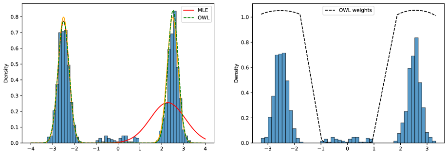
Figure 1: An example illustrating failures of maximum likelihood estimation (MLE) for misspecified models. The data were generated from an equally weighted mixture of two Gaussians with means $-2.5$ and $2.5$, and with standard deviation $1/4$. 5% of the data were corrupted by replacement with i.i.d uniform$(-1,1)$ noise. Left: The red solid line denotes the MLE found using expectation maximization. The green dashed line denotes the solution found by maximizing our optimistic weighted likelihood. The orange solid line denotes the uncorrupted density. Right: Depicted are the weights on the individual likelihood terms learned by the OWL methodology.

The origin of brittleness is intimately tied to the foundations of statistical science. Specifically, much of statistical theory and methodology assumes a domain expert capable of precisely modelling real-world phenomena. This idealised setting is sometimes referred to as the M-closed world (see Bernardo and Smith, 2009); and assumes that for a fixed but unknown parameterisation of the likelihood, we can recover the data-generating mechanism accurately. Conveniently for the statistician, this leaves computation and estimation as the only problems to be resolved. Unfortunately, the real world is not M-closed: even the most seasoned scientists often struggle with developing models that are flawless descriptions of all aspects of the data they seek to model. As a result, inferences built on this assumption are often brittle (see e.g. Lindsay, 1994; Müller, 2013; Grünwald, 2011), and the advent of large scale and high-dimensional data has only exacerbated this problem.

Perhaps the oldest strategy for addressing this is to try to explicitly model the complexities of real data settings—such as outliers and data contamination—by using a more flexible model. Often, the corresponding likelihood functions correspond to mixture models, models with heavier tails, or semiparametric and nonparametric extensions. However, as one increases the complexity of the likelihood to combat model misspecification, one creates a host of new challenges. These include decreased interpretability, problems with parameter identifiability, and increased computational complexity. In addition, even with a more complex likelihood, some degree of model misspecification remains inevitable. As a result, even highly flexible likelihoods do not provide guaranteed protection against brittleness.

This has led to a renewed interest in robust statistics: rather than trying to adjust the likelihood function, many modern approaches instead derive guarantees that continue to hold under various forms of misspecification. This includes a large potpourri of contributions, ranging from model- and algorithm-specific methods (e.g. Bhatia et al., 2023; Diakonikolas et al., 2017, 2019, 2020) to general frameworks of obtaining robustified inferences (e.g. Bissiri et al., 2016; Jewson et al., 2018; Lyddon et al., 2018; Knoblauch et al., 2022; Lecué and Lerasle, 2020). Much of the methodological work in this area has taken one of three approaches: distance-based estimation Barp et al. (2019); Knoblauch et al. (2018); Cherief-Abdellatif and Alquier (2020); Briol et al. (2019); Matsubara et al. (2022); Dellaporta et al. (2022); Alquier et al. (2022); Chérief-Abdellatif and Alquier (2022), novel means of uncertainty quantification with a Bayesian flavour Lyddon et al. (2018); Huggins and Miller (2020); Pompe and Jacob (2021); Fong et al. (2021), or modified likelihood functions Hooker and Vidyashankar (2014); Ghosh and Basu (2016); Field and Smith (1994); Windham (1995); Markatou et al. (1997); Hadi and Luceño (1997); Markatou et al. (1998); Dupuis and Morgenthaler (2002). We will propose a novel methodology that roughly falls into this last category and focuses on finding robust parameter estimates based on a modification of the likelihood function. This means that our methodology is universally applicable to both frequentist and Bayesian methods, and is easier to interpret than distance-based methods.

A particular subclass of modified likelihoods that have been of great practical interest are (locally) weighted likelihoods. For a likelihood function $f$, the weighted likelihood replaces $L(x_{1:n}|\theta)=\prod_{i=1}^{n}f(x_{i}|\theta)$ by the weighted counterpart rCl L(x_1:n—θ) & = ∏_i=1^n f(x_i—θ)^w_i for a collection of weights $\{w_{i}\}_{i=1}^{n}$ that typically are allowed to depend on the data as well as $\theta$. Weighting schemes like this have been proposed for local likelihood methods that interpolate between parameter and density estimation (Hunsberger, 1994; Copas, 1995; Hjort and Jones, 1996; Loader, 1996; Eguchi and Copas, 1998), for improving predictive performance (Shimodaira, 2000), as well as in the context of Bayesian methods (Newton and Raftery, 1994; Greco et al., 2008; Agostinelli and Greco, 2013; Lyddon et al., 2019). Motivated by robustness, re-weighting schemes first arose in the context of linear regression (see e.g. Green, 1984; Gervini and Yohai, 2002; Marazzi and Yohai, 2004). The first mentions of a general construction to enhance the robustness of arbitrary likelihoods are due to Beran (1981) and Pregibon (1982). While the weighting schemes proposed in Beran (1981) are computationally unattractive, they inspired a range of alternative schemes that also aim at robustness and are more computationally tractable (Field and Smith, 1994; Windham, 1995; Markatou et al., 1997; Hadi and Luceño, 1997; Markatou et al., 1998; Dupuis and Morgenthaler, 2002). The most important of these are density-weighted approaches (Windham, 1995) which coincide with robust distance-based estimation methods for a particular sub-class of statistical models (Basu et al., 1998), weights based on the cumulative density function and quantiles (Field and Smith, 1994; Hadi and Luceño, 1997), and weights based on Pearson residuals (Markatou et al., 1997, 1998).

While there are some asymptotic results for certain weighted likelihood constructions (Lenth and Green, 1987; Hu, 1997; Wang et al., 2004; Wang and Zidek, 2005; Majumder et al., 2021), most of these only hold if models are well-specified and under conditions that are generally hard to verify. Furthermore, while various weighted likelihood schemes have been proposed for robustness, the nature of this robustness often lacks interpretability. Beyond that, most weighting schemes are not universally applicable and rely on additional knowledge that may not be generally available. For example, the approaches of Field and Smith (1994); Hadi and Luceño (1997) rely on the availability of cumulative density functions for the statistical model underlying the likelihood function. Similarly, Markatou et al. (1997, 1998) require Pearson residuals, which are generally difficult to compute on continuous spaces.

In this paper, we introduce the optimistically weighted likelihood (OWL) methodology. This approach does not suffer the drawbacks of these previous proposals: Specifically, OWL is provably well-behaved in the asymptotic regime, guarantees robustness by means of an interpretable construction, and is universally applicable. The key intuition behind our approach is that parameter inference based on the weighted likelihood is equivalent to inference based on the standard-likelihood for a re-weighted empirical distribution. The weights are then chosen so that the re-weighted empirical measure (a) is within an $\epsilon$-neighborhood of the observed data distribution with respect to a suitable distance all while (b) being close to an element of the model class. The robustness of OWL follows from the choice of distance in (a). In particular, OWL inherits the particular robustness properties of the distance it is based on. Meanwhile, the optimism of (b) allows OWL to recover parameters that are $\epsilon$-close to the data generating distribution, if such parameters exist. In this paper, we choose the total variation (TV) distance for step (a): It is easy to interpret, is a proper metric, and is robust to outliers and contamination (see e.g. Yatracos, 1985). While it is conceptually easy to modify our methodology for alternative distances, there may be substantial computational hurdles.

Although directly inferring optimistic weights that satisfy (a) and (b) in the TV setting is intractable, we develop an alternating optimization scheme that can be easily implemented in a variety of settings. Empirically, the weights recovered by this procedure behave as theory would predict: they assign near-zero values to observations that are in strong disagreement with the likelihood model. The right panel of Figure 1 illustrates this: as theory predicts, the weights are very small on the region containing the corrupted data, and much higher on regions that produce a good fit for the posed likelihood model.

We also show that OWL is intimately connected with the principle of coarsened inference (Miller and Dunson, 2019). The coarsened likelihood is a natural generalization of standard likelihood; and posits that the empirical distribution of idealized data generated from the assumed statistical model is within a discrepancy $\epsilon$ of the empirical distribution of the observed data—rather than the two being equal, which is the assumption implicitly underlying inference for well-specified models. Despite its natural interpretation, coarsened likelihoods are difficult to evaluate or approximate directly, except in the special case when the discrepancy is chosen to be the Kullback Leibler (KL) divergence (Miller and Dunson, 2019). While directly computing coarsened likelihoods is intractable in finite samples, we use techniques from large deviation theory (Dembo and Zeitouni, 2010) to show that coarsened likelihoods converge to their corresponding optimistically weighted likelihood for a broad class of discrepancies. This result provides an alternate motivation of OWL as a tool for approximating coarsened likelihoods.

In summary, our contribution is a robust OWL methodology based on neighborhoods of the data measured in TV distance. While computing the optimal weights is generally intractable, we propose an easily implementable alternating optimization scheme to approximately solve this problem. Beyond that, we also demonstrate an asymptotic equivalence between OWL and coarsened likelihoods. The resulting inferences exhibit desirable properties, both in theory and practice.

The remainder of the paper discusses these findings as follows: Section 2 presents the OWL methodology and the associated alternating optimization scheme. Section 3 discusses the computational details of each of the steps in the alternating optimization procedure. Section 4 demonstrates the asymptotic connection between OWL and coarsened inference. Section 5 presents a suite of simulation experiments for the OWL methodology in both regression and clustering tasks. Section 6 applies the OWL methodology to a clustering application for single-cell RNAseq data. Section 7 uses the OWL methodology to estimate the average intent-to-treat effect in the micro-credit study by Angelucci et al. (2015), whose inference was shown to be brittle to the removal of an handful of observations (Broderick et al., 2020).

2 Optimistically Weighted Likelihoods

As Figure 1 shows, maximum likelihood estimation can be brittle when the data generating distribution $P_{0}$ is allowed to have a small degree of misspecification with respect to the model family $\{P_{\theta}\}_{\theta\in\Theta}$. To assuage the problem of brittleness under misspecification, we propose an Optimistically Weighted Likelihood (OWL) approach that iterates between (1) optimistically re-weighting the observed data points and (2) updating the parameter estimate by maximizing a weighted likelihood based on the current data weights.

In Section 2.1, we study this parameter inference methodology at the population level where we formally allow $P_{0}$ to be misspecified. Here we introduce the population level optimistic Kullback Leibler (OKL) function with parameter $\epsilon\in[0,1]$ (Equation 1), and show that its minimizer will be a parameter $\theta$ for which $P_{\theta}$ is $\epsilon$-close to $P_{0}$ in TV distance. Under suitable conditions, the minimization of the OKL can be performed by iterating the two steps of a) projection of the current model estimate onto the $\epsilon$ TV neighborhood around $P_{0}$ in a Kullback Leibler sense (information projection), and b) finding the parameter that maximizes a suitably weighted integral of the log likelihood.

Motivated by this population analysis, in Section 2.2, we derive the OWL-based parameter estimation methodology when only samples $x_{1},\ldots,x_{n}$ from $P_{0}$ are available.

2.1 Population level Optimistic Kullback Leibler minimization

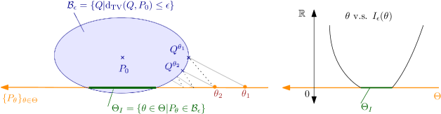
Figure 2: Population level description of OWL (left) and the OKL function (right). The point $P_{\theta}$ is labeled using $\theta\in\Theta$. The inference problem is to find a point in $\Theta_{I}\subseteq\Theta$ where the model family intersects the $\epsilon$-neighborhood $\mathcal{B}_{\epsilon}$ of the data distribution $P_{0}$. The set $\Theta_{I}$ is the set of minimizers of the OKL function $\theta\mapsto I_{\epsilon}(\theta)$ (right). Starting from initial point $\theta_{1}\in\Theta$, the OWL procedure finds a saddle point of the OKL function by iterating $\theta_{t+1}=\operatorname*{arg\,min}_{\theta\in\Theta}\operatorname{KL}(Q^{\theta_{t}}|P_{\theta})$ for $t=1,2,\ldots,$ until convergence, where $Q^{\theta}=\operatorname*{arg\,min}_{Q\in\mathcal{B}_{\epsilon}}\operatorname{KL}(Q|P_{\theta})$ denotes the information projection (Amari (2016)) of the model $P_{\theta}$ on the total variation (TV) neighborhood $\mathcal{B}_{\epsilon}$ of $P_{0}$. Iterations alternate between I-projection and weighted likelihood estimation steps, illustrated via solid and dashed lines.

Let $\mathcal{P}(\mathcal{X})$ denote the space of probability distributions on the data space $\mathcal{X}$. Our methodology can accommodate misspecification in terms of a variety of probability metrics (e.g. MMD or Wasserstein) on $\mathcal{P}(\mathcal{X})$, but here we mainly focus on the total variation (TV) distance for concreteness and interpretability. Let $\text{d}_{\text{TV}}(P,Q)=\sup_{A\subseteq\mathcal{X}}|P(A)-Q(A)|$ denote the TV metric between two probability distributions $P,Q\in\mathcal{P}(\mathcal{X})$. Given a model family $\{P_{\theta}\}_{\theta\in\Theta}\subseteq\mathcal{P}(\mathcal{X})$, we assume that the data generating distribution $P_{0}\in\mathcal{P}(\mathcal{X})$ for the data population in question satisfies $\text{d}_{\text{TV}}(P_{0},P_{\theta^{*}})\leq\epsilon$ for a known value $\epsilon\geq 0$ and some unknown $\theta^{*}\in\Theta$. In other words, we make the following assumption:

Assumption 2.1.

Given $\epsilon\geq 0$ and the true data distribution $P_{0}$, the set of parameters $\Theta_{I}=\{\theta\in\Theta|\text{d}_{\text{TV}}(P_{0},P_{\theta})\leq\epsilon\}$ is non-empty.

Assumption 2.1 encompasses Huber’s $\epsilon$-contamination model (Huber, 1964) since the condition $\text{d}_{\text{TV}}(P_{0},P_{\theta^{*}})\leq\epsilon$ follows whenever $P_{0}=(1-\epsilon)P_{\theta^{*}}+\epsilon C$, for an arbitrary contaminating distribution $C\in\mathcal{P}(\mathcal{X})$. However, Assumption 2.1 is strictly more general, since $\text{d}_{\text{TV}}(P_{0},P_{\theta^{*}})\leq\epsilon$ does not imply that $P_{0}$ is an $\epsilon$-contamination of $P_{\theta^{*}}$. Indeed, Lemma 25 in the appendix shows that for fixed $P_{0}$, $P_{\theta^{*}}$, and $\epsilon$, $P_{0}=(1-\epsilon)P_{\theta^{*}}+\epsilon C$ for some contaminating distribution $C$ if and only if the Radon Nikodym derivative $\frac{dP_{\theta^{*}}}{dP_{0}}$ exists and is bounded from above by $\frac{1}{1-\epsilon}$, $P_{0}$ almost surely.

In general, under Assumption 2.1, it may only be possible to identify the set $\Theta_{I}$, rather than any particular $\theta^{*}$. Although such indeterminacy may be inherent, it is practically insignificant whenever $\epsilon$ is sufficiently small so that the distinction between two elements from $\Theta_{I}$ is practically irrelevant (Huber, 1964). In line with this insight, the goal throughout the rest of the paper will be to identify some parameter in $\Theta_{I}$.

At the population level, usual maximum likelihood parameter estimation amounts to minimizing the Kullback Leibler (KL) function $\theta\mapsto\operatorname{KL}(P_{0}|P_{\theta})$ on the parameter space $\Theta$. Even under small amounts of misspecification, KL minimizers are very brittle. The origin of this phenomenon is that any minimizers of the KL function must place sufficient probability mass wherever $P_{0}$ does, including on outliers. In contrast, TV distance is far less sensitive to the geometry of misspecifaction. Hence one may minimize $\theta\mapsto\text{d}_{\text{TV}}(P_{0},P_{\theta})$ as a robust alternative, particularly under Assumption 2.1. However, direct minimization of TV distance over the parameter space $\Theta$ is difficult to implement in practice due to the lack of suitable optimization primitives (e.g. maximum likelihood estimators) and the non-convex and non-smooth nature of the optimization problem (see e.g. Yatracos, 1985).

An approach minimizing the KL divergence with its second argument constrained within an $\epsilon$-neighborhood under the Lévy-Prokhorov metric—as opposed to the TV distance—was proposed in Yang and Chen (2018) to provide Neyman-Pearson optimal tests for a robust version of the universal hypothesis testing problem for univariate distributions. Our motivation is estimation and inference rather than testing. Indeed, asymptotic analysis of the coarsened likelihood (Miller and Dunson, 2019) using Sanov’s theorem (see Section 4) gives rise to a similar KL objective constrained by an $\varepsilon$-neighbourhood. The resulting function, which we term the Optimistic Kullback Leibler (OKL), is defined as follows.

Definition 2.1.

(Optimistic Kullback Leibler) Given $P_{0}$ and $\epsilon>0$, the OKL function $I_{\epsilon}:\Theta\to[0,\infty]$ is defined as:

$$I_{\epsilon}(\theta)=\inf_{Q\in\mathcal{B}_{\epsilon}(P_{0})}\operatorname{KL}(Q|P_{\theta}),$$ (1)

where $\mathcal{B}_{\epsilon}(P_{0})=\{Q\in\mathcal{P}(\mathcal{X})|\text{d}_{\text{TV}}(P_{0},Q)\leq\epsilon\}$ is the TV ball of radius $\epsilon$ around $P_{0}$. If $I_{\epsilon}(\theta)<\infty$, the underlying optimization over $\mathcal{B}_{\epsilon}(P_{0})$ has a unique minimizer $Q^{\theta}$ called the I-projection (Csiszár, 1975).

The function $\theta\mapsto I_{\epsilon}(\theta)$ measures the fit of a model $P_{\theta}$ to the data $P_{0}$ allowing for a degree $\varepsilon$ of data re-interpretation in TV distance before assessing model fit. Our terminology Optimistic Kullback Leibler emphasizes that $I_{\epsilon}(\theta)$ is the KL divergence between the most optimistic re-interpretation $Q^{\theta}$ of the data within the data neighborhood $\mathcal{B}_{\epsilon}(P_{0})$ and the model distribution $P_{\theta}$. Here we use the term optimistic re-interpretation in the sense that, if $\theta$ is our current parameter estimate, our methodology calculates the KL divergence optimistically, by supposing that the true data are generated from the model-friendly distribution $Q^{\theta}$ rather than $P_{0}$. Here, $\epsilon\geq 0$ regulates the permitted degree of re-interpreting the data by controlling the neighborhood size.

The OKL function enables us to perform robust parameter inference by finding a parameter from the set $\Theta_{I}$: Since $I_{\epsilon}(\theta)=\operatorname{KL}(Q^{\theta}|P_{\theta})$, under Assumption 2.1, the minimum OKL value of zero will be attained exactly on $\Theta_{I}$ (since $Q^{\theta}=P_{\theta}$ if and only if $\theta\in\Theta_{I}$). This implies that finding a minimizer of $\theta\mapsto I_{\epsilon}(\theta)$ amounts to finding a robust parameter estimate. However, the OKL may be non-convex, so that calculating the global minimizer of OKL may not be straightforward. Fortunately, the OKL lends itself to a feasible alternating optimization scheme that will reach a saddle point under suitable conditions.

Global minimization of the OKL function is equivalent to the joint global minimization of the function $F:\Theta\times\mathcal{B}_{\epsilon}(P_{0})\to[0,\infty]$ given by $F(\theta,Q)=\operatorname{KL}(Q|P_{\theta})$, since $I_{\epsilon}(\theta)=\inf_{Q\in\mathcal{B}_{\epsilon}(P_{0})}F(\theta,Q)$. Thus we will use alternating minimization to jointly minimize the function $F$, i.e. for $t\in\mathbb{N}$ we perform the $Q$-step: $Q^{\theta_{t}}=\operatorname*{arg\,min}_{Q\in\mathcal{B}_{\epsilon}(P_{0})}\operatorname{KL}(Q|P_{\theta_{t}})$ and the $\theta$-step: $\theta_{t+1}=\operatorname*{arg\,min}_{\theta\in\Theta}\operatorname{KL}(Q^{\theta_{t}}|P_{\theta})$. For simplicity, suppose that the model family $\{P_{\theta}\}_{\theta\in\Theta}$ and $P_{0}$ have densities $\{p_{\theta}\}_{\theta\in\Theta}$ and $p_{0}$ with respect to a common measure $\lambda$, then the I-projection $Q^{\theta_{t}}$ will also have a density $q_{t}$ with respect to $\lambda$, and the iterations will take the following form. Starting from $\theta_{1}\in\Theta$ such that $I_{\epsilon}(\theta_{1})<\infty$, compute the following steps for $t\in\mathbb{N}$:

1. Q-step: Compute the I-projection of $P_{\theta_{t}}$ on the ball $\mathcal{B}_{\epsilon}(P_{0})$. This corresponds to solving a convex optimization problem over the space of probability densities $\mathscr{D}(\mathcal{X})=\{q:\mathcal{X}\to[0,\infty)\mid\int q(x)d\lambda(x)=1\}$ with respect to $\lambda$.

   $$q_{t}=\operatorname*{arg\,min}_{\begin{subarray}{c}q\in\mathscr{D}(\mathcal{X})\\ \frac{1}{2}\int|q-p_{0}|d\lambda\leq\epsilon\end{subarray}}\int q(x)\log\frac{q(x)}{p_{\theta_{t}}(x)}d\lambda(x).$$

2. $\theta$-step: Maximize the average log-likelihood $\theta\mapsto\int q_{t}(x)\log p_{\theta}(x)d\lambda(x)$. Note that $\operatorname{KL}(Q^{\theta_{t}}|P_{\theta})=\int q_{t}(x)\log q_{t}(x)d\lambda(x)-\int q_{t}(x)\log p_{\theta}(x)d\lambda(x)$ with the convention that $0\log 0=0$. Hence the optimization step $\theta_{t+1}=\operatorname*{arg\,min}_{\theta\in\Theta}\operatorname{KL}(Q^{\theta_{t}}|P_{\theta})$ can be re-written as:

   $$\theta_{t+1}=\operatorname*{arg\,max}_{\theta\in\Theta}\int q_{t}(x)\log p_{\theta}(x)d\lambda(x).$$

The above iterations provide a scheme to minimize the OKL function in which the $Q$-step can approximately be performed using tools from convex optimization, while the $\theta$-step can be approximated by maximization of a suitably weighted log-likelihood, which can be computed for many standard models. Our resulting population level methodology is illustrated in Figure 2.

Assuming that there is always a unique minimizer in the $\theta$-step, it is straightforward to show that the objective value $F(\theta_{t},Q^{\theta_{t}})$ is a strictly decreasing function of $t$ as long as $\theta_{t}\neq\theta_{t+1}$. Thus if $\{\theta_{t}\}_{t\in\mathbb{N}}$ lie in a compact set and suitable continuity assumptions hold, any limit point $\tilde{\theta}$ of the sequence $\{\theta_{t}\}_{t\in\mathbb{N}}$ will satisfy the saddle point condition $\tilde{\theta}=\operatorname*{arg\,min}_{\theta\in\Theta}\operatorname{KL}(Q^{\tilde{\theta}}|P_{\theta})$. This saddle point condition is satisfied by all the parameters in the identifiable set $\Theta_{I}$.

We remark that one can use optimization of the OKL function $I_{\epsilon}(\theta)$ as a subroutine to minimize the function $\theta\mapsto\text{d}_{\text{TV}}(P_{0},P_{\theta})$. Namely, we can perform binary search over $\epsilon\in[0,1]$, increasing $\epsilon$ whenever we have $I_{\epsilon}(\theta)>0$ and decreasing $\epsilon$ whenever we have $I_{\epsilon}(\theta)=0$. Used this way, OKL optimization can be seen as a computationally-palatable approach to minimizing the TV distance over a model class.

2.2 Optimistically Weighted Likelihood (OWL) estimation

We now extend the population level methodology from Section 2.1 to handle the practical case when samples $x_{1},\ldots,x_{n}\overset{i.i.d.}{\sim}P_{0}$ are available, and provide a computable approximation for the $Q$-step and $\theta$-step from Section 2.1. Namely, the $Q$-step (now called $w$-step) will be approximated by a suitable convex optimization problem over weights that lie within the intersection of an $n$-dimensional probability simplex and the $\ell_{1}$ ball of radius $2\epsilon$ around the vector with uniform weights; these optimal weights can be interpreted as an optimistic re-weighting of the original data points $x_{1},\ldots,x_{n}$ to match the current model estimate. Further, the $\theta$-step will then be approximated by maximizing a weighted likelihood with the weights found in the previous step. Since this methodology involves the repeated steps of parameter estimation using a weighted likelihood (i.e. the $\theta$-step) and re-estimating the weights on the data points to optimistically match the estimated model (i.e. the $w$-step), we call this the Optimistically Weighted Likelihood (OWL) method.

2.2.1 Approximating OKL by a finite dimensional optimization problem

We derive the OWL methodology by approximating the OKL function $I_{\epsilon}(\theta)$ in terms of a finite dimensional optimization problem defined in terms of observed data $x_{1},\ldots,x_{n}\overset{i.i.d.}{\sim}P_{0}$. Henceforth, let us assume that the model family $\{P_{\theta}\}_{\theta\in\Theta}$ and measure $P_{0}$ have densities $\{p_{\theta}\}_{\theta\in\Theta}$ and $p_{0}$ with respect to a common measure $\lambda$. We will focus on two cases of interest: when $\mathcal{X}$ is a finite space and $\lambda$ is the counting measure, and when $\mathcal{X}=\mathbb{R}^{d}$ and $\lambda$ is the Lebesgue measure.

When $\mathcal{X}$ is finite, we look to solve the optimization problem in eq. 1 over data re-weighting $Q=\sum_{i=1}^{n}w_{i}\delta_{x_{i}}$ as the weight vector $w=(w_{1},\ldots,w_{n})$ varies over the $n$-dimensional probability simplex $\Delta_{n}$ and satisfies the TV constraint $\frac{1}{2}\|w-o\|_{1}\leq\epsilon$ where $o=(1/n,\ldots,1/n)\in\Delta_{n}$ is the vector with uniform weights. Formally, our finite space OKL approximation is given by

$$\hat{I}_{\epsilon,\textnormal{fin}}(\theta)=\inf_{\begin{subarray}{c}w\in{\Delta}_{n}\\ \frac{1}{2}\|w-o\|_{1}\leq\epsilon\end{subarray}}\sum_{i=1}^{n}w_{i}\log\frac{nw_{i}\hat{p}_{\textnormal{fin}}(x_{i})}{p_{\theta}(x_{i})},$$ (2)

where $\hat{p}_{\textnormal{fin}}(y)=\frac{|\{i\in[n]|x_{i}=y\}|}{n}$ is the histogram estimator for the data generating distribution $p_{0}$ when $\mathcal{X}$ is a finite space. An application of the log sum inequality (Cover and Thomas, 2006, Theorem 2.7.1) shows that the weights that solve eq. 2 have the appealing and natural property that $w_{i}=w_{j}$ whenever $x_{i}=x_{j}$. Moreover, when the support of $p_{0}$ contains the support of $p_{\theta}$, $\hat{I}_{\epsilon,\textnormal{fin}}(\theta)$ converges to $I_{\epsilon}(\theta)$ at rate $n^{-1/2}$, as demonstrated by the following result.

Theorem 1.

Suppose that $I_{\epsilon_{0}}(\theta)<\infty$ for some $\epsilon_{0}>0$ and pick $\delta>0$ and $\epsilon>\epsilon_{0}$. If $\operatorname{supp}(p_{\theta})\subseteq\operatorname{supp}(p_{0})$ and $x_{1},\ldots,x_{n}\overset{i.i.d.}{\sim}p_{0}$, then with probability at least $1-\delta$,

$$|I_{\epsilon}(\theta)-\hat{I}_{\epsilon,\textnormal{fin}}(\theta)|\leq O\left(\frac{|\operatorname{supp}(p_{0})|}{\epsilon-\epsilon_{0}}\sqrt{\frac{1}{n}\log\frac{|\operatorname{supp}(p_{0})|}{\delta}}\right),$$

where $\operatorname{supp}(p)=\{x\in\mathcal{X}:p(x)>0\}$.

See Appendix B for the proof and a more general theorem statement with explicit constants.

When $\mathcal{X}=\mathbb{R}^{d}$, the above approximation strategy needs to be modified, since $\operatorname{KL}(Q|P_{\theta})$ is unbounded whenever $P_{\theta}$ is supported on all of $\mathcal{X}$ and $Q=\sum_{i=1}^{n}w_{i}\delta_{x_{i}}$ is a discrete distribution. In this case, eq. 1 should be formulated in terms of measures $Q\in\mathcal{P}(\mathcal{X})$ that have density $q$ with respect to $\lambda$. Namely, we start with the formulation:

$$I_{\epsilon}(\theta)=\inf_{\begin{subarray}{c}q\in\mathscr{D}(\mathcal{X})\\ \frac{1}{2}\int|q-p_{0}|d\lambda\leq\epsilon\end{subarray}}\int q(x)\log\frac{q(x)}{p_{\theta}(x)}d\lambda(x)$$ (3)

where $\mathscr{D}(\mathcal{X})=\{q:\mathcal{X}\to[0,\infty)\mid\int q(x)d\lambda(x)=1\}$ is the space of probability densities with respect to $\lambda$. Next, using a suitable probability kernel $\kappa:\mathcal{X}\times\mathcal{X}\to[0,\infty)$, we restrict the domain of the optimization problem in eq. 3 to the finite dimensional subspace of densities $\{q_{v}|v\in\Delta_{n}\}$, where $q_{v}(\cdot)\doteq\sum_{i=1}^{n}v_{i}\kappa(x_{i},\cdot)$ denotes the probability density indexed by weight vector $v\in\Delta_{n}$. As an example, we may use the Gaussian kernel $\kappa(x,y)=\frac{1}{(2\pi\sigma^{2})^{d/2}}\exp(-\frac{\|x-y\|^{2}}{2h^{2}})$ for a bandwidth parameter $h>0$.

For a probability kernel $\kappa$, using the finite dimensional approximation $\{q_{v}:v\in\Delta_{n}\}$ for the space of densities, and a suitable Monte Carlo approximation to the integral objective in eq. 3, we obtain the approximation:

$$\hat{I}_{\epsilon}(\theta)=\inf_{\begin{subarray}{c}w\in\hat{\Delta}_{n}\\ \frac{1}{2}\|w-o\|_{1}\leq\epsilon\end{subarray}}\sum_{i=1}^{n}w_{i}\log\frac{nw_{i}\hat{p}(x_{i})}{p_{\theta}(x_{i})}$$ (4)

where $\hat{p}$ is a suitable density estimator for $p_{0}$ based on $x_{1},\ldots,x_{n}$, $A$ is an $n\times n$ matrix with entries $A_{ij}=\frac{\kappa(x_{i},x_{j})}{n\hat{p}(x_{i})}$, and $\hat{\Delta}_{n}=A\Delta_{n}$ is the image of the $n$-dimensional probability simplex under linear operator $A$. We will typically take $\hat{p}(\cdot)=\frac{1}{n}\sum_{j=1}^{n}\kappa(\cdot,x_{j})$ to be the kernel-density estimate based on the same kernel $\kappa$, in which case $A$ is the stochastic matrix obtained by normalizing the rows of the kernel matrix $K=(\kappa(x_{i},x_{j}))_{i,j\in[n]}$ to sum to one.

The continuous space approximation in eq. 4 yields the finite space approximation in eq. 2 as a special case when $\kappa(x,y)=I\{x=y\}$ is taken to be the indicator kernel. The weights vectors in $\hat{\Delta}_{n}$ are always non-negative and approximately sum to one for large values of $n$, since $\sum_{i=1}^{n}A_{ij}=\frac{1}{n}\sum_{i=1}^{n}\frac{\kappa(x_{i},x_{j})}{\hat{p}(x_{i})}\approx\int\frac{\kappa(x,x_{j})}{\hat{p}(x)}p_{0}(x)dx\approx 1$. The derivation of eq. 4 along with large sample consistency can be found in Appendix C, but we briefly describe the main result here.

Proving the convergence of $\hat{I}_{\epsilon}(\theta)$ is technically challenging, as it requires proving uniform-convergence of the objective in eq. 4 when the weights are allowed to vary over the entire range $\hat{\Delta}_{n}$. To get around this, we restrict the optimization domain to $\hat{\Delta}_{n}^{\beta}=A\Delta_{n}^{\beta}$ where $\Delta_{n}^{\beta}=\{(v_{1},\ldots,v_{n})\in\Delta_{n}\,:\,v_{i}\in[\frac{\beta}{n},\frac{1}{n\beta}]\}$ for a suitably small constant $\beta$. Thus, the estimator that we theoretically study is given by

$$\hat{I}_{\epsilon,\beta}(\theta)=\inf_{\begin{subarray}{c}w\in\hat{\Delta}_{n}^{\beta}\\ \frac{1}{2}\|w-o\|_{1}\leq\epsilon\end{subarray}}\sum_{i=1}^{n}w_{i}\log\frac{nw_{i}\hat{p}(x_{i})}{p_{\theta}(x_{i})}.$$ (5)

Given this change, we can show the following result.

Theorem 2.

Suppose $\operatorname{supp}(p_{0})=\operatorname{supp}(p_{\theta})=\mathcal{X}$ is a compact subset of $\mathbb{R}^{d}$ and there exists a constant $\gamma>0$ such that $p_{0}(x),p_{\theta}(x)\in[\gamma,1/\gamma]$ for all $x\in\mathcal{X}$. Suppose that we use the probability kernel $\kappa(x,y)=\frac{1}{h^{d}}\phi(\|x-y\|/h)$ having bandwidth $h>0$, with $\kappa$ positive semi-definite and $\phi$ bounded above by a constant and having exponentially-decaying tails. Assume that $p_{0}$ and $\log p_{\theta}$ are $\alpha$-Hölder smooth over $\mathcal{X}$, and suppose that we use the clipped density estimator $\hat{p}(x)=\min(\max(\frac{1}{n}\sum_{i=1}^{n}\kappa(x_{i},x),\gamma),1/\gamma)$. Then for any constant $0<\beta\leq\gamma^{2}/4$

$$\left|\hat{I}_{\epsilon,\beta}(\theta)-I_{\epsilon}(\theta)\right|\leq\tilde{O}\left(n^{-1/2}h^{-d}+h^{\alpha/2}+\psi(\sqrt{h})\right),$$

with probability at least $1-1/n$, where $\psi(r)=\frac{\lambda(\mathcal{X}\setminus\mathcal{X}_{-r})}{\lambda(\mathcal{X})}$, $\lambda(\cdot)$ is the $d$-dimensional Lebesgue measure, $\mathcal{X}_{-r}=\{x\in\mathcal{X}:B(x,r)\subseteq\mathcal{X}\}$, and $\tilde{O}(\cdot)$ hides constants and logarithmic factors.

Observe that $\psi(r)$ measures the fraction of the volume of $\mathcal{X}$ that is contained in the envelope of width $r$ closest to the boundary. For well-behaved sets, we expect $\psi(r)$ to decrease to 0 as $r\rightarrow 0$. For example, if $\mathcal{X}$ is a $d$-dimensional ball of radius $r_{0}$, then $\psi(r)=1-(1-\frac{r}{r_{0}})^{d}$.

We prove our theory with the truncated estimator $\hat{I}_{\epsilon,\beta}(\theta)$ instead of $\hat{I}_{\epsilon}(\theta)$ for techincal reasons. By a suitable version of the sandwiching lemma (Section A.2), under the assumptions of Theorem 2, we conjecture that the optimal weights in (4) lie in the set $\hat{\Delta}^{\beta}_{n}$ for a small enough constant $\beta>0$, in which case we will have $\hat{I}_{\epsilon,\beta}(\theta)=\hat{I}_{\epsilon}(\theta)$.

2.2.2 OWL Methodology

With a computable approximation $\hat{I}_{\epsilon}$ (or $\hat{I}_{\epsilon,\textnormal{fin}}$) to the OKL function in hand, we follow the alternating minimization strategy described in Section 2.1 to minimize the function $\theta\mapsto\hat{I}_{\epsilon}(\theta)$. In more detail, we replace the density $q_{t}$ (or more precisely the relative density $w=q_{t}/p_{0}$) in the $Q$-step with the weight vector $w_{t}=(w_{t,1},\ldots,w_{t,n})\in\mathbb{R}_{\geq 0}^{n}$ that minimizes eq. 4 for $\hat{I}_{\epsilon}(\theta_{t})$. We rename this the $w$-step to emphasize the new setup. Next, the $\theta$-step corresponds to minimizing the function $\theta\mapsto\sum_{i=1}^{n}w_{t,i}\log\frac{nw_{t,i}\hat{p}(x_{i})}{p_{\theta}(x_{i})}$, which is equivalent to maximizing the weighted likelihood $\theta\mapsto\sum_{i=1}^{n}w_{t,i}\log p_{\theta}(x_{i})$.

The resulting procedure is summarized in Algorithm 1. In Section 3, we expand on the computational details for the $\theta$-step and $w$-steps, but note for now that the $w$-step involves solving a convex optimization problem for which standard tools are available, while the $\theta$-step corresponds to maximizing a weighted likelihood, which can be performed for many models through simple modifications of procedures for the corresponding maximum likelihood estimation.

Finally, it is straightforward to see that the iterates $\theta_{t}$ of Algorithm 1 must decrease the objective function $\theta\mapsto\hat{I}_{\epsilon}(\theta)$, as we have

$$\hat{I}_{\epsilon}(\theta_{t+1}) =\sum_{i=1}^{n}w_{t+1,i}\log\frac{nw_{t+1,i}\hat{p}(x_{i})}{p_{\theta_{t+1}}({x}_{i})}\leq\sum_{i=1}^{n}w_{t,i}\log\frac{nw_{t,i}\hat{p}(x_{i})}{p_{\theta_{t+1}}({x}_{i})}$$

$$\leq\sum_{i=1}^{n}w_{t,i}\log\frac{nw_{t,i}\hat{p}(x_{i})}{p_{\theta_{t}}({x}_{i})}=\hat{I}_{\epsilon}(\theta_{t}).$$

Since eq. 4 is a convex optimization problem with a strictly convex objective, the first inequality is strict unless $w_{t+1}=w_{t}$. Hence the objective $\hat{I}_{\epsilon}$ must decrease strictly at each step.

Algorithm 1 OWL Methodology

Input: Model $\{p_{\theta}\}_{\theta\in\Theta}$, coarsening parameter $\epsilon\geq 0$, probability kernel $\kappa$, initial point $\theta_{1}\in\Theta$, and iteration limit $T$.

for $t=1,\ldots,T$ do

   $w$-step: Find $w_{t}=(w_{t,1},\ldots,w_{t,n})\in\mathbb{R}_{\geq 0}^{n}$ that minimizes eq. 4 for $\theta=\theta_{t}$.

   $\theta$-step: Find $\theta_{t+1}$ that maximizes the weighted likelihood $\theta\mapsto\sum_{i=1}^{n}w_{t,i}\log p_{\theta}(x_{i})$.

end for

Output: The robust parameter estimate $\theta_{T}$ and the data weights $w_{T}$.

In practice, when the data lie in a continuous space, we often avoid using the kernel-based estimator eq. 4 to determine the weights in the $w$-step of Algorithm 1 because it greatly slows down the computation (see Section 3.1), and the resulting weights are sensitive to the choice of kernel $\kappa$. Instead, setting $\kappa(x,y)=I\{x=y\}$, we perform the $w$-step by solving the unkernelized optimization problem:

$$\min_{\begin{subarray}{c}w\in\Delta_{n}\\ \frac{1}{2}\|w-o\|_{1}\leq\epsilon\end{subarray}}\Big{\{}-\sum_{i=1}^{n}w_{i}\log p_{\theta}(x_{i})+\sum_{i=1}^{n}w_{i}\log w_{i}\Big{\}},$$

obtained from eq. 4 when all the data points $x_{1},\ldots,x_{n}$ are distinct. We demonstrate in Section 5.1 that the unkernelized version of the OWL procedure has equally good performance compared to the kernelized version with a suitably tuned bandwidth. A potential explanation for this is that the primary role of the $w$-step is to down-weight outliers under the model density $p_{\theta}$, which is controlled by the first term in the optimization objective above; in contrast, the second term in the optimization objective controls the regularity of the non-outlying weights, and plays a secondary role in the $w$-step.

2.2.3 Setting the corruption fraction $\epsilon$

So far we have assumed that the parameter $\epsilon\in(0,1)$, which can be interpreted as the fraction of corrupted samples in the population distribution, is fixed at a known value that satisfies Assumption 2.1. Now let us see how the population level analysis (Section 2.1) can inform our choice of $\epsilon$. Assumption 2.1 is satisfied as long as $\epsilon\geq\varepsilon_{0}$, where

$$\varepsilon_{0}=\min_{\theta\in\Theta}\text{d}_{\text{TV}}(P_{0},P_{\theta})=\left\{\epsilon\in[0,1]:\min_{\theta\in\Theta}I_{\epsilon}(\theta)=0\right\}.$$

Hence, in principle, we could set $\epsilon=\varepsilon_{0}$ to use OWL to perform minimum-TV estimation (Yatracos, 1985), which has the following advantages: (1) while directly minimizing TV distance is computationally intractable, the OWL methodology decomposes this problem into alternating convex optimization and weighted MLE steps, both of which are standard problems that often tend to be well-behaved, and (2) the OWL methodology provides us with weight vectors that can indicate outlying observations and relates minimum TV-estimation to likelihood based inference.

In order to choose $\epsilon\approx\varepsilon_{0}$ in practice, we define the function $\hat{g}(\epsilon)=\hat{I}_{\epsilon}(\hat{\theta}_{\epsilon})$, where $\hat{\theta}_{\epsilon}$ is the parameter estimate computed by the OWL procedure for a given $\epsilon$. At the population level, the corresponding function $g(\epsilon)=\min_{\theta\in\Theta}I_{\epsilon}(\theta)$ is monotonically decreasing in $\epsilon$ until $\epsilon=\varepsilon_{0}$, at which point it remains at 0. This introduces a kink, or elbow, at $\epsilon_{0}$ that we hope to identify in the sample estimate $\hat{g}$. Thus, our $\epsilon$-search procedure is to compute $\hat{g}$ over a fixed grid of $\epsilon$-values, smooth the resulting grid, and then select amongst the points of largest curvature (computed numerically), where the curvature of a twice-differentiable function $f$ at a point $x$ is given by $f^{\prime\prime}(x)/(1+f^{\prime}(x)^{2})^{1.5}$ (Satopaa et al., 2011). Despite the various approximations involved, our simulation results (Section 5) show that the OWL procedure with such a tuned value of $\epsilon$ provides almost identical performance when compared with the OWL procedure with the true value of $\epsilon$.

2.3 OWL extension to non-identically-distributed data

While the population level analysis and theoretical results for the OKL estimator were derived under the assumption that data are generated i.i.d. from a distribution $P_{0}$, the OWL procedure can be adapted to robustify likelihood based inference in the setting where the data are conditionally independent, but not necessarily identically distributed.

Suppose data $z_{1},\ldots,z_{n}\in\mathcal{Z}$ are conditionally independent, with the likelihood having the product form $p_{\theta}(z_{1:n})=\prod_{i=1}^{n}p_{\theta,i}(z_{i})$, for known functions $\{p_{\theta,i}\}_{i=1}^{n}$. For example, if $z_{i}=(y_{i},x_{i})\in\mathbb{R}\times\mathcal{X}$ for $i=1,\ldots,n$, this includes the case of regression models $\{q_{\theta}(y|x)\}_{\theta\in\Theta}$ under the setup $p_{\theta,i}(z_{i})=q_{\theta}(y_{i}|x_{i})$. Another example of this setup includes mixture models if we expand the parameter space to also include cluster assignments (see Section 3.2.2).

To robustify inference based on the product likelihood $p_{\theta}(z_{1:n})=\prod_{i=1}^{n}p_{\theta,i}(z_{i})$, we can replace the $w$- and $\theta$- steps in Algorithm 1 by analogous steps in the product likelihood case. In particular, the modified $w$-step is given by

$$w_{t}=\operatorname*{arg\,min}_{\begin{subarray}{c}w\in\Delta_{n}\\ \frac{1}{2}\|w-o\|_{1}\leq\epsilon\end{subarray}}\left\{-\sum_{i=1}^{n}w_{i}\log p_{\theta_{t},i}(x_{i})+\sum_{i=1}^{n}w_{i}\log w_{i}\right\}$$

and the modified $\theta$-step is given by

$$\theta_{t+1}=\operatorname*{arg\,min}_{\theta\in\Theta}\sum_{i=1}^{n}w_{t,i}\log p_{\theta,i}(x_{i}).$$

Despite our lack of theory in the non-identically-distributed case, we continue to see good empirical performance of the OWL estimator in this setup when evaluated on synthetic data (see Section 5).

3 Performing OWL computations

In this section, we expand on the computational details of the OWL methodology. Specifically, in Section 3.1 we discuss our approach to solving the constrained convex optimization problems in eqs. 2 and 4, and in Section 3.2 we discuss the details of optimizing a weighted likelihood for exponential families and mixture models.

3.1 Computing the $w$-step (I-projection)

3.1.1 Unkernelized I-projection

Suppose that $\mathcal{X}$ is finite. Then the finite approximation to the OKL of eq. 2 is given by the solution to the convex optimization problem

$$\min_{\begin{subarray}{c}w\in{\Delta}_{n}\\ \frac{1}{2}\|w-o\|_{1}\leq\epsilon\end{subarray}}\sum_{i=1}^{n}w_{i}\log\frac{w_{i}n_{i}}{p_{\theta}(x_{i})},$$

where $n_{i}=|\{j:x_{j}=x_{i}\}|$ is the number of times that $x_{i}$ occurs in our sample.

This is a convex optimization problem for which there are a number of candidate solutions. Our approach is based on (consensus) Alternating Direction Method of Multipliers (ADMM) (Boyd et al., 2011; Parikh and Boyd, 2014). To frame the OKL optimization problem in the language of ADMM, we rewrite it as

$$\min_{w\in\mathbb{R}^{n}}\overbrace{\sum_{i=1}^{n}w_{i}\log\frac{w_{i}n_{i}}{p_{\theta}({x}_{i})}}^{f_{1}(w)}+\overbrace{i_{\{w\in\Delta_{n}\}}}^{f_{2}(w)}+\overbrace{i_{\{\frac{1}{2}\|w-o\|_{1}\leq\epsilon\}}}^{f_{3}(w)},$$ (6)

where $i_{\{C\}}$ is 0 whenever the condition $C$ is true and $\infty$ otherwise. Written in this form, ADMM boils down to implementing the individual proximal operators for the $f_{i}$’s, where the proximal operator of a closed proper convex function $f:\mathbb{R}^{n}\rightarrow\mathbb{R}$ and parameter $\lambda>0$ is defined as the function

$$\operatorname{prox}_{\lambda f}(x)=\operatorname*{arg\,min}_{z\in\mathbb{R}^{n}}\left\{f(z)+\frac{1}{2\lambda}\|z-x\|_{2}^{2}\right\}.$$

In our setting, the proximal operator for the KL term $f_{1}$ can be computed element-wise using the Lambert-W function (Barratt et al., 2021), or in log-scale via the Wright omega function, for which fast algorithms exist (Lawrence et al., 2012), leading to $O(n)$ computational complexity. The proximal operator for $f_{2}$ corresponds to projection onto the $n$-dimensional scaled probability simplex, which can be computed in $O(n)$ time (Condat, 2016). The proximal operator for $f_{3}$ corresponds to projection onto an $\ell_{1}$-ball, and in fact it can be reduced to projection onto the simplex (Condat, 2016).

To simplify our discussion on the implementation of ADMM, we rewrite eq. 6 for an arbitrary number of convex functions $f_{1},\ldots,f_{k}:\mathbb{R}^{n}\rightarrow\mathbb{R}$ as

$$\min_{\begin{subarray}{c}w^{(1)},\ldots,w^{(k)},z\in\mathbb{R}^{n}\\ w^{(i)}=z\text{ for all }i\end{subarray}}\sum_{i=1}^{k}f_{i}\left(w^{(i)}\right).$$

For penalty parameters $\lambda_{1},\ldots,\lambda_{k}>0$, the augmented Langrangian associated with this problem is given by

$$L\left(w^{(1:k)},y^{(1:k)},z\right)=\sum_{i=1}^{k}f_{i}\left(w^{(i)}\right)+\langle y^{(i)},w^{(i)}-z\rangle+\frac{1}{2\lambda_{i}}\|w^{(i)}-z\|^{2},$$

where $w^{(1)},\ldots,w^{(k)}\in\mathbb{R}^{n}$ are the primal variables, $y^{(1)},\ldots,y^{(k)}\in\mathbb{R}^{n}$ are the dual variables, and $z\in\mathbb{R}^{n}$ is the consensus variable. Then the consensus ADMM algorithm is derived by iteratively optimizing the augmented Langrangian coordinate-wise. That is, starting from some initialization $w^{(i,0)},y^{(i,0)},z^{(0)}\in\mathbb{R}^{n}$, we perform the following updates

$$w^{(i,t+1)} =\operatorname*{arg\,min}_{w^{(i)}\in\mathbb{R}^{n}}L\left(w^{(-i,t+1)},w^{(i)},y^{(1:k,t+1)},z^{(t)}\right)=\operatorname{prox}_{\lambda_{i}f_{i}}\left(z^{(t)}+\lambda_{i}y^{(i,t)}\right)$$

$$z^{(t+1)} =\operatorname*{arg\,min}_{z\in\mathbb{R}^{n}}L\left(w^{(1:k,t+1)},y^{(1:k,t+1)},z\right)=\frac{1}{\sum_{i=1}^{k}1/\lambda_{i}}\sum_{i=1}^{k}\left(\frac{1}{\lambda_{i}}w^{(i,t+1)}-y^{(i,t)}\right)$$

$$y^{(i,t+1)} =y^{(i,t)}+\frac{1}{\lambda_{i}}(z^{(t+1)}-w^{(i,t+1)}).$$

Algorithm 2 displays the full consensus ADMM algorithm. In our implementation, we use the self-adaptive rule suggested by He et al. (2000) to independently update each of the penalty parameters.

Algorithm 2 Consensus ADMM to compute the I-projection

Input: Proximal operators $\operatorname{prox}_{\lambda f_{i}}$ for functions in eq. 6, dimension $n$, number of iterations $T$, and proximal penalty parameters $\lambda_{i}>0$.

Initialize $w_{i}^{0},y_{i}^{0},z^{0}=\vec{0}\in\mathbb{R}^{n}$ for $i=1,2,3$.

for $t=0,\ldots,T-1$ do

   Set $w^{(i,t+1)}=\operatorname{prox}_{\lambda_{i}f_{i}}(z^{(t)}+\lambda_{i}y^{(i,t)})$ for $i=1,2,3$.

   Set $z^{(t+1)}=\frac{1}{\sum_{i=1}^{k}1/\lambda_{i}}\sum_{i=1}^{k}\left(w^{(i,t+1)}/\lambda_{i}-y^{(i,t)}\right)$.

   Set $y^{(i,t+1)}=y^{(i,t)}+(z^{(t+1)}-w^{(i,t+1)})/\lambda_{i}$ for $i=1,2,3$.

   Optionally, adjust $\lambda_{i}$ for $i=1,2,3$.

end for

Output: $w_{1}^{T}$.

3.1.2 Kernelized I-projection

In the Euclidean case with $\mathcal{X}=\mathbb{R}^{d}$, beyond the sample $x_{1},\ldots,x_{n}$ and parameter $\theta\in\Theta$, we additionally have a kernel matrix $K\in\mathbb{R}^{n\times n}$ with induced row sums $s_{i}=\sum_{j}K_{ij}$ and row-normalized matrix $A_{ij}=K_{ij}/s_{i}$. The optimization problem of eq. 4 translates to

$$\min_{v\in\mathbb{R}^{n}}\sum_{i=1}^{n}(Av)_{i}\log\frac{(Av)_{i}s_{i}}{p_{\theta}({x}_{i})}+i_{\{v\in\Delta^{n}\}}+i_{\{\frac{1}{2}\|Av-o\|_{1}\leq\epsilon\}}.$$ (7)

Although all the terms in eq. 7 remain convex in $v$, the proximal operators for the KL objective and the $\ell_{1}$ constraint are no longer available in closed form. To circumvent this issue, we can rewrite problems of this form as

$$\min_{\begin{subarray}{c}w^{(1)},\ldots,w^{(k)},z\in\mathbb{R}^{n}\\ w^{(i)}=M_{i}z\text{ for all }i\end{subarray}}\sum_{i=1}^{k}f_{i}\left(w^{(i)}\right),$$

where each $M_{i}\in\mathbb{R}^{n\times n}$. The augmented Langrangian in this case becomes

$$L\left(w^{(1:k)},y^{(1:k)},z\right)=\sum_{i=1}^{k}f_{i}\left(w^{(i)}\right)+\langle y^{(i)},w^{(i)}-M_{i}z\rangle+\frac{1}{2\lambda_{i}}\|w^{(i)}-M_{i}z\|^{2},$$

which leads to the ADMM updates

$$w^{(i,t+1)} =\operatorname{prox}_{\lambda_{i}f_{i}}\left(M_{i}z^{(t)}+\lambda_{i}y^{(i,t)}\right)$$

$$z^{(t+1)} =\left(\sum_{i=1}^{k}M_{i}^{T}M_{i}/\lambda_{i}\right)^{-1}\sum_{i=1}^{k}M_{i}^{T}\left(w^{(i,t+1)}/\lambda_{i}-y^{(i,t)}\right)$$

$$y^{(i,t+1)} =y^{(i,t)}+\frac{1}{\lambda_{i}}(M_{i}z^{(t+1)}-w^{(i,t+1)}).$$

In our setting, each $M_{i}$ is either equal to $A$ or to the identity matrix $I$. Thus, the matrix inverse in the update of $z$ can be computed efficiently using a single singular value decomposition of $A$, even if the penalty parameters change between iterations. To see this, suppose that $A=U\textnormal{diag}(\sigma_{1},\ldots,\sigma_{n})V^{T}$ is the SVD of $A$ and let $J=\{i:M_{i}=A\}$. Then the $z$ update can be written as

$$z^{(t+1)}=V\textnormal{diag}\left((\beta_{J^{c}}+\sigma_{1}^{2}\beta_{J})^{-1},\ldots,(\beta_{J^{c}}+\sigma_{n}^{2}\beta_{J})^{-1}\right)V^{T}\sum_{i=1}^{k}M_{i}^{T}\left(w^{(i,t+1)}/\lambda_{i}-y^{(i,t)}\right),$$

where $\beta_{J}=\sum_{i\in J}\lambda_{i}^{-1}$ and $\beta_{J^{c}}=\sum_{i\not\in J}\lambda_{i}^{-1}$.

3.1.3 Computational complexity and generalization to other distances

As mentioned above, each of the three proximal operators in eq. 6 and eq. 7 can be implemented in $O(n)$ time. For the non-kernelized version of the ADMM algorithm in Algorithm 2, the remaining linear algebraic steps can also be implemented in $O(n)$ time, bringing the total computational complexity of the procedure to $O(Tn)$, where $T$ is the number of ADMM steps taken. For the kernelized version of the ADMM algorithm, we require an SVD computation as a preprocessing step, which takes $O(n^{3})$ time, and each step additionally involves matrix-vector products, taking time $O(n^{2})$. Thus, the total time complexity of the kernelized ADMM procedure amounts to $O(n^{3}+Tn^{2})$, which is polynomial in $n$ but not feasible for large values of $n$.

We remark here that from an optimization perspective, for both eqs. 6 and 7, the $\ell_{1}$-distance is not special. We may substitute in any distance that is convex in its arguments and for which there are computationally efficient methods for projection onto the corresponding balls with a specified center and radius. This includes $\ell_{2}$-distance, whose projection can be computed by a simple shift and rescaling, and maximum mean discrepancy (Gretton et al., 2006) whose projection operator is onto an ellipsoid and can be reduced to a one-dimensional root finding problem (Kiseliov, 1994).

3.2 Computing the $\theta$-step: maximizing weighted likelihoods

We now shift focus to the second step in the OWL procedure, maximizing a weighted likelihood:

$$\max_{\theta\in\Theta}\sum_{i=1}^{n}w_{i}\log p_{\theta}({x}_{i}).$$

We will expand on this problem for two settings: exponential families and mixture models.

3.2.1 Weighted maximum likelihood for exponential families

Consider the setting where $p_{\theta}$ is an exponential family and $\Theta\subset\mathbb{R}^{d}$ is the natural parameter space so that

$$p_{\theta}(x)=h(x)\exp\left(\theta^{T}T(x)-A(\theta)\right),$$

where $T:\mathcal{X}\rightarrow\mathbb{R}^{d}$ is a sufficient statistic, $h$ is a base measure, and $A:\theta\rightarrow\mathbb{R}$ is the log-normalizing factor. Then for $w\in\Delta_{n}$, the weighted maximization step solves

$$\max_{\theta\in\Theta}\sum_{i=1}^{n}w_{i}\log p_{\theta}({x}_{i})=\min_{\theta\in\Theta}\left\{A(\theta)-\theta^{T}\sum_{i=1}^{n}w_{i}T(x_{i})\right\}.$$ (8)

This solution satisfies the gradient condition $\nabla A(\theta)=\sum_{i=1}^{n}w_{i}T(x_{i}).$

For exponential families, whenever $\operatorname{Cov}(T(X))$ is positive definite for $X\sim p_{\theta}$, the function $\nabla A(\theta)$ is invertible. Thus, this step can be solved quickly whenever we can compute the inverse of $\nabla A(\cdot)$. When $\operatorname{Cov}(T(X))$ is not strictly positive definite, or more generally when the inverse of $\nabla A(\cdot)$ is not available in closed form, the objective in eq. 8 is still convex in $\theta$ and can be solved using tools from convex optimization.

3.2.2 Weighted maximum likelihood for mixture models

In the mixture model setting, the parameters $\theta$ encode mixing weights $\pi\in\Delta_{K}$ and component parameters $\phi_{1},\ldots,\phi_{K}\in\Phi$ such that $p_{\phi}$ denotes a probability density over $\mathcal{X}$. Then the likelihood under $\theta$ can be written as

$$p_{\theta}(x_{1:n})=\prod_{i=1}^{n}\left(\sum_{k=1}^{k}\pi_{k}p_{\phi_{k}}(x_{i})\right).$$

To compute the maximum likelihood estimate, it is standard to introduce latent categorical random variables $z_{i}\stackrel{{\scriptstyle iid}}{{\sim}}\pi$, $z_{i}\in\{1,\ldots,K\},i=1,\ldots,n,$ and rewrite the likelihood as

$$p_{\theta}(x_{1:n})=\mathbb{E}_{z\sim\pi}\left[\prod_{i=1}^{n}p_{\phi_{z_{i}}}(x_{i})\right].$$

The above can then be maximized using the EM algorithm (Dempster et al., 1977). Unfortunately, the introduction of weights into the likelihood no longer allows for an easy decomposition via these latent variables.

However, consider the likelihood with respect to the augmented latent variables $\tilde{\theta}=(\theta,z_{1:n})\in\tilde{\Theta}$:

$$p_{\tilde{\theta}}(x_{1:n})=\prod_{i=1}^{n}p_{\phi_{z_{i}}}(x_{i}).$$

Then, following the setup from Section 2.3, the weighted log-likelihood can be written as

$$\sum_{i=1}^{n}w_{i}\log p_{\phi_{z_{i}}}(x_{i})=\sum_{k=1}^{K}\sum_{i:z_{i}=k}w_{i}\log p_{\phi_{k}}(x_{i}).$$

Thus, to maximize the above for fixed latent variables $z_{1},\ldots,z_{n}$, we can maximize the weighted log-likelihood of the individual component parameters over its assigned (weighted) data. For many component distributions (e.g., Gaussians, Poissons), this can be computed in closed-form. On the other hand, for fixed component variables $\phi_{1},\ldots,\phi_{k}$, we can maximize this weighted log-likelihood over the $z_{1},\ldots,z_{n}$ by assigning each data point to the component that maximizes its individual likelihood. This suggests the following scheme, reminiscent of the ‘hard EM’ algorithm (Samdani et al., 2012):

$$\phi_{k}^{t+1} =\operatorname*{arg\,max}_{\phi\in\Phi}\sum_{i:z^{t}_{i}=k}w_{i}\log p_{\phi}(x_{i})\text{ for each }k=1,\ldots,K$$

$$z_{i}^{t+1} =\operatorname*{arg\,max}_{k\in\{1,\ldots,K\}}\log p_{\phi_{k}}(x_{i})\text{ for each }i=1,\ldots,n.$$

In general, optimizing over the augmented parameter space $\tilde{\Theta}$ implicitly assumes a generative model different from the one assumed by optimizing over $\Theta$. In particular, when one optimizes over $\Theta$, the assumed generative model is that the data come from some distribution $P_{0}$ that is $\epsilon$-close to $P_{\theta}$ for some $\theta\in\Theta$. The implied generative model when optimizing over $\tilde{\Theta}$ is that the data come from some mixture distribution $\sum_{k}\pi_{k}p_{k}$ such that each component $p_{k}$ is $\epsilon$-close to some $\phi_{k}\in\Phi$. For most settings, the first generative model is a strict generalization of the second. However, in the $\epsilon$-contamination model, these are equivalent, as implied by the following result.

Proposition 1.

Let $P_{0},P_{1},\ldots,P_{K}$ denote probability measures, $\pi\in\Delta_{K}$, and $\epsilon>0$. Then the following are equivalent.

• There exists a probability measure $Q$ such that $P_{0}=(1-\epsilon)\sum_{k=1}^{K}\pi_{k}P_{k}+\epsilon Q$.

• There exist probability measures $Q_{1},\ldots,Q_{k}$ such that $P_{0}=\sum_{k=1}^{K}\pi_{k}((1-\epsilon)P_{k}+\epsilon Q_{k})$.

The proof of Proposition 1 follows from simple algebraic substitution.

4 Asymptotic connection to coarsened inference

The development of the OWL methodology in Section 2 followed from a presumed form of misspecification given by Assumption 2.1. An alternative way to frame and address such misspecifications in a probabilistic framework was proposed by Miller and Dunson (2019) who introduced Bayesian methodology centered around the concept of a coarsened likelihood defined as

$$L_{\epsilon}(\theta|x_{1:n})\doteq\mathbb{P}_{\theta}\left(\boldsymbol{d}(\hat{P}_{Z_{1:n}},\hat{P}_{x_{1:n}})\leq\epsilon\right),$$ (9)

where $\boldsymbol{d}$ is a suitably chosen discrepancy between empirical probability measures. Here, $\hat{P}_{x_{1:n}}=n^{-1}\sum_{i=1}^{n}\delta_{x_{i}}$ denotes the empirical distribution of data $x_{1:n}$, and the probability is computed under $\mathbb{P}_{\theta}$—the distribution underlying the artificial data $Z_{1},\ldots Z_{n}\overset{i.i.d.}{\sim}P_{\theta}$ from which the random measure $\hat{P}_{Z_{1:n}}=n^{-1}\sum_{i=1}^{n}\delta_{Z_{i}}$ is constructed. The coarsened likelihood implicitly captures the likelihood of a probabilistic procedure in which idealized data are first generated by some model $\mathbb{P}_{\theta}$ in the model class under consideration, but are then corrupted in such a way that the discrepancy between empirical measures of the idealized data and the observed data is bounded by $\epsilon$.

When $\boldsymbol{d}$ is an estimator for the KL-divergence and an exponential prior is placed on $\epsilon$, Miller and Dunson (2019) showed that the Bayes posterior based on $L_{\epsilon}(\theta|x_{1:n})$ could be approximated by raising the likelihood to a power less than one in the formula for the standard posterior. However, to obtain a robustified alternative to maximum likelihood estimation, one may wish to maximize $\theta\mapsto L_{\epsilon}(\theta|x_{1:n})$ directly for a choice of $\boldsymbol{d}$ that guarantees robustness (e.g. Maximum Mean Discrepancy or the TV distance). Such an approach would in general be quite challenging since evaluating eq. 9 corresponds to computing a high-dimensional integral.

In this section, we show that for large $n$, the coarsened likelihood can be approximately maximized by using the OWL methodology when $\boldsymbol{d}$ is an estimator for the TV distance. Specifically, if the observed data $x_{1},\ldots,x_{n}$ are generated i.i.d. from some distribution $P_{0}$ and $\boldsymbol{d}$ satisfies appropriate regularity conditions, then the negative rescaled coarsened likelihood $-\frac{1}{n}\log L_{\epsilon}(\theta|x_{1:n})$ asymptotically converges as $n\to\infty$ to a variant of $I_{\epsilon}(\theta)$ based on $\boldsymbol{d}$. Hence, the OWL methodology asymptotically maximizes the coarsened likelihood $\theta\mapsto L_{\epsilon}(\theta|x_{1:n})$. In Sections 4.1 and 4.2, we develop this asymptotic connection for finite and continuous spaces, respectively. All proofs for this section can be found in Appendix D.

4.1 Asymptotic connection in finite spaces

Let $\mathcal{X}$ be a finite set and denote the space of probability distributions on $\mathcal{X}$ by the simplex $\Delta_{\mathcal{X}}\doteq\{q\in[0,1]^{\mathcal{X}}|\sum_{x\in\mathcal{X}}q(x)=1\}$. Let $\{p_{\theta}\}_{\theta\in\Theta}\subseteq\Delta_{\mathcal{X}}$ denote the collection of model distributions, and $p_{0}\in\Delta_{\mathcal{X}}$ denote the true data generating distribution. To establish connection of OKL with the coarsened likelihood eq. 9, we will take $\boldsymbol{d}(p,q)=\frac{1}{2}\|p-q\|_{1}$ to be the TV distance.

Given this setting, we can show that $-\frac{1}{n}\log L_{\epsilon}(\theta|x_{1:n})$ converges in probability to the OKL function $I_{\epsilon}(\theta)$ at rate $n^{-1/2}$, as demonstrated by the following theorem.

Theorem 3.

Suppose that $I_{\epsilon_{0}}(\theta)<\infty$ for some $\epsilon_{0}>0$ and let $\delta>0$. If $\epsilon>\epsilon_{0}$ and $x_{1},x_{2},\ldots,x_{n}\overset{i.i.d.}{\sim}p_{0}$, then with probability at least $1-\delta$,

$$\left|I_{\epsilon}(\theta)+\frac{1}{n}\log L_{\epsilon}(\theta|x_{1:n})\right|\leq O\left(\frac{|\mathcal{X}|}{\epsilon-\epsilon_{0}}\sqrt{\frac{1}{n}\log\frac{1}{\delta}}+\frac{|\mathcal{X}|}{n}\left(|\mathcal{X}|+\log(n)+\frac{1}{\epsilon-\epsilon_{0}}\right)\right).$$

Our proof hinges on analyzing a quantity that is closely related to $L_{\epsilon}(\theta|x_{1:n})$:

$$M_{n,\epsilon}(\theta)=\mathbb{P}_{Z_{1},\ldots Z_{n}\overset{i.i.d.}{\sim}p_{\theta}}\left(\frac{1}{2}\|\hat{P}_{Z_{1:n}}-p_{0}\|_{1}\leq\epsilon\right).$$

Instead of looking at the distance to the empirical estimator $\hat{P}_{x_{1:n}}$ as in $L_{\epsilon}(\theta|x_{1:n})$, the quantity $M_{n,\epsilon}(\theta)$ considers the distance to the distribution $p_{0}$ itself. This simplifies matters greatly, and allows us to establish the following result, which is essentially a consequence of Sanov’s theorem from large deviation theory (Dembo and Zeitouni, 2010).

Lemma 1.

If $I_{\epsilon_{0}}(\theta)<\infty$ for some $\epsilon_{0}>0$, then

$$\left|I_{\epsilon}(\theta)+\frac{1}{n}\log M_{n,\epsilon}(\theta)\right|\leq{O}\left(\frac{|\mathcal{X}|}{n}\left(|\mathcal{X}|+\log(n)+\frac{1}{\epsilon-\epsilon_{0}}\right)\right)$$

for all $\epsilon>\epsilon_{0}$.

The rest of the proof of Theorem 3 amounts to establishing that $L_{\epsilon}(\theta|x_{1:n})$ is close to $M_{n,\epsilon}(\theta)$, which follows from continuity arguments and the fact that $\hat{P}_{x_{1:n}}$ converges to $p_{0}$ in $\ell_{1}$ distance.

Theorem 1 and Theorem 3 together show that, in the large sample limit, the OWL methodology and coarsened likelihood philosophy are two sides of the same coin: they both provide approximations of the OKL and, in turn, must approximate each other.

4.2 Asymptotic connection in continuous spaces

Suppose $\mathcal{X}=\mathbb{R}^{d}$ and $\mathscr{D}(\mathcal{X})$ denotes the set of densities on $\mathcal{X}$ with respect to the Lebesgue measure. Let $\{p_{\theta}\}_{\theta\in\Theta}\subseteq\mathscr{D}(\mathcal{X})$ denote the set of model densities and let $p_{0}$ denote the density of the data generating measure $P_{0}$.

Similar to the finite case, we can use Sanov’s theorem from Large Deviation theory to establish the following asymptotics for the coarsened likelihood for a suitable class of discrepancies $\boldsymbol{d}$, which includes the Wasserstein distance, Maximum Mean Discrepancy with suitable choice of kernels (Simon-Gabriel and Schölkopf, 2018), and the smoothed TV distance (Definition 4.1).

Theorem 4.

Suppose $I_{\epsilon_{0}}(\theta)<\infty$ for some $\epsilon_{0}>0$ and $\boldsymbol{d}:\mathcal{P}(\mathcal{X})\times\mathcal{P}(\mathcal{X})\to[0,\infty)$ is a pseudometric that is convex in its arguments and continuous with respect to the weak convergence topology on $\mathcal{P}(\mathcal{X})$. If $\epsilon>\epsilon_{0}$ and $x_{1},\ldots,x_{n}\overset{i.i.d.}{\sim}P_{0}$, then

$$-\frac{1}{n}\log L_{\epsilon}(\theta|x_{1:n})\xrightarrow{P}\inf_{\begin{subarray}{c}Q\in\mathcal{P}(\mathcal{X})\\ \boldsymbol{d}(Q,P_{0})\leq\epsilon\end{subarray}}\operatorname{KL}(Q|P_{\theta})\quad\text{ as $n\to\infty$.}$$

Recall that the limiting expression in the above theorem has the same form as that of the OKL function given in eq. 3. However, in order to establish connection between the OKL function and the coarsened likelihood, unlike in the finite case, we cannot merely take the discrepancy $\boldsymbol{d}$ in the coarsened likelihood to be the TV distance, since the TV distance between the two empirical distributions in eq. 9 will almost surely be equal to one. Instead, we will take $\boldsymbol{d}$ to be a smoothed version of TV distance calculated by first convolving the empirical measures with a smooth kernel function $K_{h}:\mathcal{X}\times\mathcal{X}\to[0,\infty)$ indexed by a bandwidth parameter $h>0$.

To formally define the smoothed TV distance, let $\phi\in\mathscr{D}(\mathcal{X})$ be a continuous and bounded probability density function (e.g. standard Gaussian density), let $h>0$ be a bandwidth parameter. Then the kernel $K_{h}:\mathcal{X}\times\mathcal{X}\to[0,\infty)$ is defined as $K_{h}(x,y)=\frac{1}{h^{d}}\phi((x-y)/h)$, and for any measure $\mu\in\mathcal{P}(\mathcal{X})$, the convolved density $K_{h}\star\mu\in\mathscr{D}(\mathcal{X})$ is defined as $(K_{h}\star\mu)(x)=\int K_{h}(x,y)\mu(dy)$.

Definition 4.1.

Given two measures $\mu,\nu\in\mathcal{P}(\mathcal{X})$ and bandwidth $h>0$, the smoothed total variation (TV) distance is defined as:

$$\text{d}_{\text{TV,}h}(\mu,\nu)=\frac{1}{2}\int|(K_{h}\star\mu)(x)-(K_{h}\star\nu)(x)|dx.$$

We extend the notion of smoothed TV distance $\text{d}_{\text{TV,}h}(p,q)=\text{d}_{\text{TV,}h}(\mu,\nu)$ to densities $p,q\in\mathscr{D}(\mathcal{X})$ based on their induced measures $\mu,\nu\in\mathcal{P}(\mathcal{X})$.

We show in Section D.2.2 that $\boldsymbol{d}=\text{d}_{\text{TV,}h}$ satisfies conditions of Theorem 4. Further, when $\phi$ has fast tail-decay and densities $p,q\in\mathscr{D}(\mathcal{X})$ satisfy appropriate regularity conditions, standard results on kernel density estimation (e.g. Rinaldo and Wasserman (2010); Jiang (2017)) show the pointwise convergence of densities $K_{h}\star q\to q$ as $h\to 0$. This, when combined with Scheffe’s lemma and the triangle inequality, shows that $\lim_{h\to 0}\text{d}_{\text{TV,}h}(p,q)=\text{d}_{\text{TV}}(p,q)$. In other words, for suitably small bandwidth parameter $h>0$, the neighborhoods based on the smoothed total variation distance approximate those based on the total variation distance.

Thus, by invoking Theorem 4 with the choice $\boldsymbol{d}=\text{d}_{\text{TV,}h}$, one expects $-\frac{1}{n}\log L_{\epsilon}(\theta|x_{1:n})\approx I_{\epsilon}(\theta)$ when $n$ is large and $h$ is small. As in the finite setting, we again see that maximizing the coarsened likelihood is closely related to minimizing the OKL function in the large sample regime. Hence the OWL methodology can be used to approximately maximize the coarsened likelihood when $\boldsymbol{d}=\text{d}_{\text{TV,}h}$ for large sample size $n$ and a suitably small bandwidth $h$. In fact for many other metrics $\boldsymbol{d}$ satisfying the conditions of Theorem 4, one can adapt the OWL methodology to maximize the function $\theta\mapsto L_{\epsilon}(\theta|x_{1:n})$ as $n\to\infty$.

5 Simulation Examples

We now turn to applications of the optimistic weighted likelihood methodology in simulated examples with artificially-injected corruptions. In each simulation, we considered two methods for choosing the points to corrupt: (i) max-likelihood corruption where we fit a maximum likelihood estimate to the uncorrupted data and select the points with the highest likelihood; and (ii) random corruption where we choose the points to corrupt uniformly at random. For clarity and space, we only present the results for max-likelihood corruptions in this section, and we defer the results for randomly-selected corruptions to Appendix F. Unless otherwise stated, the $w$-step for the OWL solutions was computed using the finite approximation to the OKL in eq. 2.

In all comparisons, OWL refers to our methodology with the data based choice of the corruption fraction $\epsilon$ as described in Section 2.2.3, while OWL ($\epsilon$ known) refers to our methdology with $\epsilon$ equal to the true level of corruption in the data. For the other robust estimation methods requiring hyperparameters, we either used commonly-accepted values (as in Huber regression), or we set them based on knowledge of the true corruption fraction (as in RANSAC regression). In all settings, we measured the performance of the maximum-likelihood estimator (MLE) that was fit using the entire uncorrupted dataset as a gold-standard benchmark.

5.1 Gaussian simulations

To investigate the performance of the OWL methodology with and without kernelization, we fit a multivariate normal distribution with mean $\mu\in\mathbb{R}^{p}$ and covariance matrix $\Sigma\in\mathbb{R}^{p\times p}$. We make two observations about this setting. First, maximizers of the weighted log-likehood can be computed in closed form, removing optimization difficulties. Second, this simple problem setting falls squarely within the i.i.d. framework of Section 2.

We generated synthetic datasets for dimensions $p=2$, 25, and 50, by drawing $\mu^{\star}_{1},\ldots,\mu^{\star}_{p}$ independently from the uniform distribution over $[-10,10]$ and drawing the uncorrupted data points independently from the spherical Gaussian $\mathcal{N}(\mu^{\star},I_{p})$, where $\mu^{*}=(\mu^{*}_{1},\ldots,\mu^{*}_{p})$. The corrupted data points had coordinates drawn independently from the uniform distribution over $[-10,10]$. The total size of the training set was set to 200. We measured the mean-squared error reconstruction of $\mu^{\star}$, i.e. for parameter estimates $\hat{\mu}\in\mathbb{R}^{p}$ and $\hat{\Sigma}\in\mathbb{R}^{p\times p}$:

$$\text{mean-parameter-mse}(\hat{\mu},\hat{\Sigma};\mu^{\star})=\frac{1}{p}\|\hat{\mu}-\mu^{\star}\|_{2}^{2}=\frac{1}{p}\sum_{i=1}^{p}(\hat{\mu}_{i}-\mu^{\star}_{i})^{2}.$$

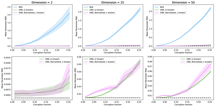
Figure 3: Gaussian results for max-likelihood corruptions. Dashed black line denotes average performance of MLE on full uncorrupted dataset. Shaded regions denote 95% confidence intervals over 50 random seeds.

For the kernelized OWL procedure, we used the Gaussian/RBF kernel: $K_{h}(x,y)=(2\pi h)^{-p/2}\exp(-\frac{1}{2h}\|x-y\|^{2})$. We adaptively set the bandwidth by searching over a fixed grid and using the final parameter’s OKL estimator in eq. 4 as the criterion to be minimized. To focus only on the role of kernelization, we set the corruption fraction $\epsilon$ equal to the true level of corruption in the dataset.

Figure 3 shows the results for the Gaussian simulations. Across the range of dimensions, both kernelized and un-kernelized OWL perform much better than MLE. Moreover, the performance of OWL without kernelization is comparable to that of OWL with kernelization. This is somewhat surprising, as our theory currently cannot explain why one should be able to run OWL in continuous spaces without some form of density estimation. For the rest of this section, we will only consider OWL without kernelization.

5.2 Regression simulations

We applied OWL to two regression settings: linear regression and logistic regression.

Linear regression.

We considered a homoscedastic model with parameters $b,\sigma^{2}\in\mathbb{R}$, $w\in\mathbb{R}^{p}$ and observations $(x_{i},y_{i})\in\mathbb{R}^{p+1}$ assumed to follow the distribution

$$y_{i}\sim\mathcal{N}(\langle x_{i},w\rangle+b,\sigma^{2}).$$

The maximizers of the weighted likelihood can be computed in closed form, as in the unweighted setting. In addition to the standard least-squares maximum likelihood estimate (MLE), we compared with (1) Ridge regression, with L2 penalty chosen via cross validation; (2) Huber regression, using the Huber penalty of 1.345 (Huber, 1981); and (3) Random Sample Consenus (RANSAC) linear regression.

We compared these methods on two datasets. The first is a simulated dataset with 10-dimensional i.i.d. standard normal covariates. The ground-truth regression coefficients $w^{\star}_{1},\ldots,w^{\star}_{10}$ were drawn independently from $N(0,4)$, and the residual standard deviation was $\sigma=1/4$. The training set consisted of 1,000 data points. For the test set, we drew 1,000 new data points and computed the MSE on the underlying response value, i.e.

$$\text{mse}(x_{1},\ldots,x_{n};\hat{w},\hat{b})\ =\ \frac{1}{n}\sum_{i=1}^{n}(\langle w^{\star},x_{i}\rangle-\langle\hat{w},x_{i}\rangle+\hat{b})^{2}.$$

The second dataset was taken from a quantitative structure activity relationship (QSAR) dataset compiled by Olier et al. (2018) from the ChEMBL database. It consists of 5012 chemical compounds whose activities were measured on the epidermal growth factor receptor protein erbB1. The activities were recorded as the negative log of the chemical concentration that inhibited 50% of the protein target, i.e. the pIC₅₀ value. Each compound had 1024 associated binary covariates, corresponding to the 1024-dimensional FCFP4 fingerprint representation of the molecule (Rogers and Hahn, 2010). We used PCA to reduce the dimension to 50. For every random seed, we computed a random 80/20 train/test split. The test MSE on this dataset is the standard MSE over the test responses. In both datasets, for each data point selected to be corrupted, we corrupted the responses by fitting a least squares solution and observing the residuals: if the residual is positive, we set the response to be $3v$ where $v$ is the largest absolute value observed value in the training set responses, otherwise setting it to $-3v$.

Figure 4 shows the results of the linear regression simulations for the max-likelihood corruptions. Across both datasets, we see that OWL is competitive with the best of the robust regression methods, whether that method is RANSAC or Huber regression.

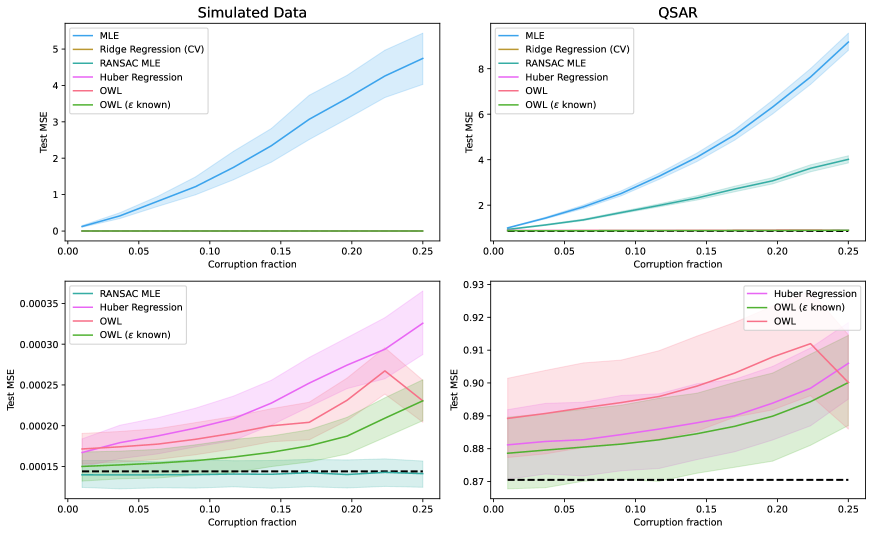
Figure 4: Linear regression results for max-likelihood corruptions. Dashed black line denotes average performance of MLE on full uncorrupted training set. Shaded regions denote 95% confidence intervals over 50 random seeds.

Logistic regression.

For the logistic regression setting, we have parameters $b,\sigma^{2}\in\mathbb{R}$, $w\in\mathbb{R}^{p}$ and observations $(x_{i},y_{i})\in\mathbb{R}^{p+1}$ assumed to follow the distribution

$$y_{i}\sim\text{Bernoulli}\left(\frac{1}{1+\exp\left(-\langle x_{i},w\rangle-b\right)}\right).$$

In addition to the standard maximum likelihood estimate (MLE), we compared against two other baselines: (i) L2-regularized MLE, with L2 penalty chosen via cross validation. (ii) Random Sample Consenus (RANSAC) logistic regression.

We compared these methods on three datasets. The first is a simulated dataset using the same parameters as the linear regression setting. The training labels are created according to the generative model. For test accuracy, we computed the zero-one loss over the true sign-values, i.e.

$$\text{accuracy}(x_{1},\ldots,x_{n};\hat{w},\hat{b})\ =\ \frac{1}{n}\#\left\{i\,:\,\mathop{\mathrm{sign}}(\langle w^{\star},x\rangle)=\mathop{\mathrm{sign}}\left(\langle\hat{w},x\rangle+\hat{b}\right)\right\}.$$

The second dataset is taken from the MNIST handwritten digit classification dataset (LeCun et al., 1998). We considered the problem of classifying the digit ‘1’ v.s. the digit ‘8,’ resulting in a dataset with 14702 data points and 784 covariates, representing pixel intensities. The third dataset is a collection of 5172 documents from the Enron spam classification dataset, preprocessed to contain 5116 covariates, representing word counts (Metsis et al., 2006). For both the MNIST and the Enron spam datasets, we reduced the dimensionality to 10 via PCA and used a random 80/20 train/test split.

Figure 5 shows the results of the logistic regression simulations. Across all datasets, we again see that OWL outperforms the other approaches in the presence of both corruption and misspecification.

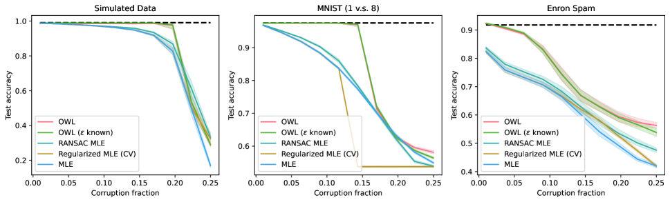
Figure 5: Logistic regression results for max-likelihood corruption. Dashed black line denotes average performance of MLE on full uncorrupted training set. Shaded regions denote 95% confidence intervals over 50 random seeds.

5.3 Mixture model simulations

We applied OWL to two mixture modeling settings: mixtures of spherical Gaussians and mixtures of Bernoulli products.

Gaussian mixture models.

Recall the standard Gaussian mixture modeling setup: there are a collection of means $\mu_{1},\ldots,\mu_{K}\in\mathbb{R}^{p}$, standard deviations $\sigma_{1},\ldots,\sigma_{K}>0$, and mixing weights $\pi\in\Delta^{K}$. Data points $x_{i}\in\mathbb{R}^{p}$ are drawn i.i.d. according to

$$x_{i}\sim\sum_{k=1}^{K}\pi_{k}\mathcal{N}(\mu_{k},\sigma_{k}^{2}I_{p}).$$

For our simulations, we generated a synthetic dataset of 1000 points in $\mathbb{R}^{10}$ by first drawing $K=3$ means $\mu^{\star}_{1},\ldots,\mu^{\star}_{K}$ whose coordinates are i.i.d. Gaussian with standard deviation 2. The standard deviations of the component Gaussians were set to $1/2$, and the mixing weights were uniform. We compared against MLE on the corrupted data. As a metric, we measured the average mean squared Euclidean distance between the means of the fitted model and the ground truth model. To corrupt a data point, we randomly selected half of its coordinates and set them randomly to either a large positive value or a large negative value (here, 10 and -10).

Because the likelihood function of a Gaussian mixture model is non-concave, the EM algorithm is only guaranteed to converge to a local optimum. Thus, for maximum likelihood estimation we used EM with random restarts, choosing the final model to be the one with largest likelihood. For the OWL procedure, we also used random restarts with the alternating optimization algorithm of Section 3. To choose the final model, we selected the one whose weights $w$ and parameters $\theta$ minimized the OKL estimator of eq. 2.

The left panel of Figure 6 shows the results of the Gaussian mixture model simulations. We see that OWL remains robust against varying levels of corruptions.

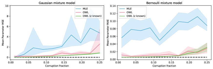
Figure 6: Mixture model results for max-likelihood corruptions. Dashed black line denotes average performance of MLE on full uncorrupted training set. Shaded regions denote 95% confidence intervals over 50 random seeds.

Bernoulli product mixture models.

Consider the following model for $p$-dimensional binary data: there are a collection of probability vectors $\lambda_{1},\ldots,\lambda_{K}\in[0,1]^{p}$ and mixing weights $\pi\in\Delta^{K}$. Each data point $x_{i}$ is drawn i.i.d. according to the process

$$z_{i} \sim\text{Categorical}(\pi)$$

$$x_{ij} \sim\text{Bernoulli}(\lambda_{z_{i}j})\text{ for }j=1,\ldots,p.$$

For our simulations, we generated a synthetic dataset of 1000 points in $\{0,1\}^{100}$ by first drawing $K=3$ means $\lambda^{\star}_{1},\ldots,\lambda^{\star}_{K}$ whose coordinates are i.i.d. from a Beta$(1/10,1/10)$ distribution. The mixing weights were chosen to be uniform over the components. As a metric, we measured the average mean $\ell_{1}$-distance between the $\lambda$ parameters of the fitted model and the ground truth model.

To corrupt a data point, we flipped each zero coordinate with probability 1/2. The right panel of Figure 6 shows the results of the Bernoulli mixture model simulations. We see that OWL remains robust against varying levels of corruptions.

6 Application to scRNA-seq Clustering

In this section, we apply our OWL methodology to a single-cell RNA sequencing (scRNA-seq) clustering problem. The GSE81861 cell line dataset (Li et al., 2017) contains single-cell RNA expression data for 630 cells from 7 cell lines across 57,241 genes. We followed the preprocessing steps of Chandra et al. (2020): we dropped cells with low reads, normalized according to Lun et al. (2016), and dropped uninformative genes with M3Drop (Andrews and Hemberg, 2019). After preprocessing, the dataset contains 531 cells and 7666 genes. Table 1 shows the breakdown of the remaining cells across cell lines. Finally, we used PCA to project down to 10 dimensions. We implemented OWL using a mixture of general Gaussians, $\sum_{k=1}^{K}\pi_{k}\mathcal{N}(\mu_{k},\Sigma_{k})$, using the same optimization procedure as in the clustering simulations of Section 5.

Cell line	A549	GM12878	H1	H1437	HCT116	IMR90	K562
Counts	74	126	164	47	51	23	46

Table 1: Breakdown of samples in GSE81861 dataset by cell line.

6.1 Cluster recovery with OWL

We measured the ability of OWL to recover the ground-truth clustering of samples. For baseline methods, we compared against maximum likelihood estimation with the same model class and K-means. As a metric of cluster recovery, we measured the adjusted Rand index (ARI) (Rand, 1971; Hubert and Arabie, 1985). In all our comparisons, we fixed the number of clusters for all methods to be 7, the number of ground truth cell lines.

The left panel of Figure 7 shows the ARI for OWL over a range of values for the $\ell_{1}$ radius parameter $\epsilon$, where we also display the performance of MLE and K-means for comparison. We see that OWL performs best when $\epsilon$ takes on values between $0.25$ and $0.45$, but generally has reasonable performance when $\epsilon$ is not too large. Moreover, we see that performance of OWL varies smoothly as a function of $\epsilon$, which may reflect the continuity of the OKL function with respect to $\epsilon$ predicted by our theory.

Figure 8 shows Uniform Manifold Approximation and Projection (UMAP) visualizations of the dataset clustered under the various methods (for one arbitrary run). We see that of all the methods, K-means performs worst by a significant margin. The improved performance of OWL (with $\epsilon=0.25$) over MLE can be mostly attributed to the better resolution the boundary between the K562 and GM12878. However, all methods struggle to identify the IMR90 cell lines as a cluster distinct from K562.

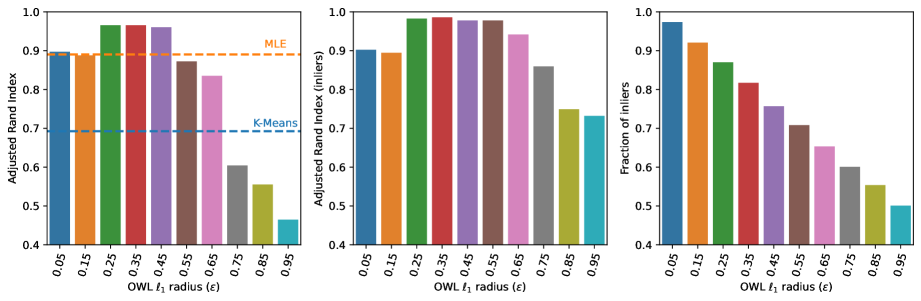
Figure 7: Comparison of clustering methods. Left: Adjusted Rand index (ARI) over the entire dataset for each of the methods. Middle: ARI of inliers for the OWL methods. Right: Fraction of data points classified as inliers for the OWL methods.

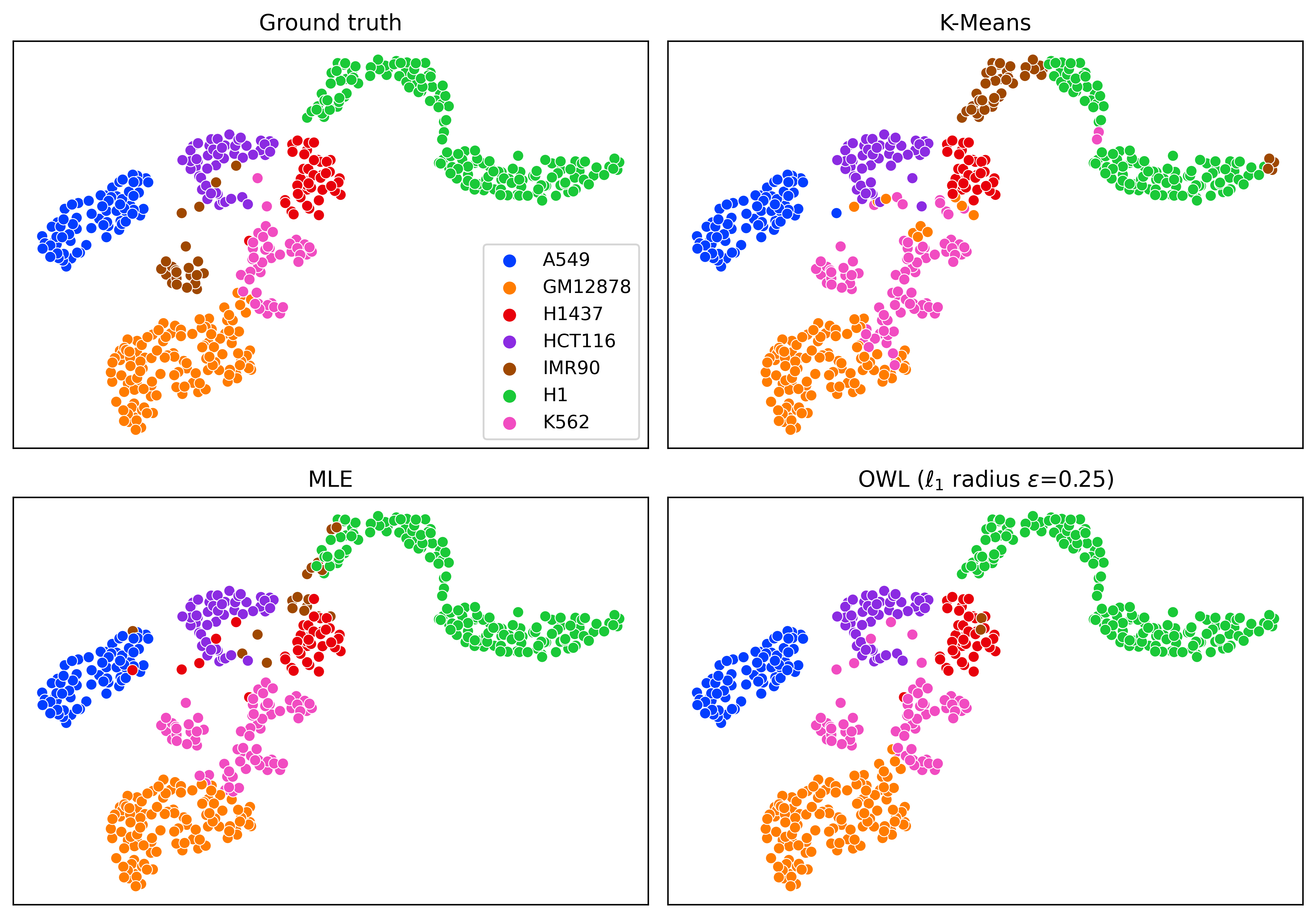
Figure 8: UMAP plots of the GSE81861 dataset under the considered clustering algorithms. Top left displays the ground truth cell lines. For the other panels, colors were selected by maximizing agreement with the ground truth clustering.

6.2 Exploratory analysis with OWL

In some settings, it is desirable to segment a dataset into those data points that are well-described by a model in the class (so-called inliers) and those that do not conform well to the model class (outliers). One interpretation of the weights that are learned by the OWL procedure is that, subject to the constraint that they are close in TV distance to the empirical distribution, they represent the most optimistic reweighting of the data relative to the model class. Thus, one might suspect that data points with higher weights are inliers and those with lower weights are outliers. Here, we explore inlier/outlier detection with OWL weights by classifying all data points with weights less than $1/n$ (the average value) as outliers, and the remainder as inliers.

The middle panel of Figure 7 shows the ARI of the OWL procedure when we restrict to the detected inliers. We observe that for all values of $\epsilon$, the ARI is no lower on the selected inliers than on the whole dataset, and in some cases is significantly higher. This suggests that the OWL procedure identifies a ‘core’ set of points that are both well-described by a mixture of Gaussians as well as aligned with the ground truth clustering. The right panel of Figure 7 shows the fraction of data points that are classified as inliers. Although it is theoretically possible for the OWL weights to classify anywhere from 1 to $n-1$ points as outliers for any value of $\epsilon$, we see that the fraction of outliers is relatively small for low values of $\epsilon$ and only increases gradually as $\epsilon$ increases.

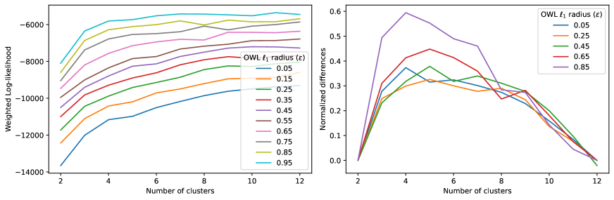
Figure 9: Left: Weighted log-likehood of the data for various settings of $\epsilon$ and the number of clusters. Right: Normalized difference graph of the weighted log-likehood function for select values of $\epsilon$. The kneedle algorithm chooses the value with the largest corresponding normalized difference.

OWL $\ell_{1}$ radius ($\epsilon$)	0.05	0.15	0.25	0.35	0.45	0.55	0.65	0.75	0.85	0.95
Selected $K$	6	6	8	7	7	7	5	4	4	4

Table 2: Number of clusters chosen by the kneedle method as a function of the $\ell_{1}$ radius $\epsilon$.

In many settings, the number of ground truth clusters are not known a priori. A common way to deal with this problem is to plot a metric such as sum-of-squares errors or log-likelihood and look for ‘elbows’ or ‘knees’ in the graph where there are diminishing returns for increasing model capacity. Here, we apply the ‘kneedle’ algorithm (Satopaa et al., 2011) to the weighted log-likehood produced by the OWL procedure. The kneedle algorithm computes the normalized differences of a given function and selects the value that maximizes the corresponding normalized differences. Figure 9 shows both the weighted log-likelihoods as well as a subset of the normalized difference graphs. Table 2 shows the selected numbers of clusters for various values of $\epsilon$. We see that for relatively small values of $\epsilon$, this results in number of clusters that is close to the ground truth. While for larger values of $\epsilon$, this procedure underestimates the number of clusters in the data. This agrees with the observation in the right panel of Figure 7 that larger values of $\epsilon$ result in fewer points being identified as inliers, and thus fewer clusters are needed to describe those points.

7 Application to micro-credit study

In this section we apply the OWL methodology to data from a micro-credit study (Angelucci et al., 2015) for which standard methods of parameter inference have been shown to be brittle to the removal of a handful of observations (Broderick et al., 2020). In Angelucci et al. (2015) the authors conducted a (clustered) randomized trial in Mexico to study the impact of availability of micro-credit on outcome measures in the community including micro-entrepreneurship, income, labor supply, consumption, social status, and subjective well-being. The authors worked with Compartamos Banco, one of the largest micro-lenders in Mexico, to randomize their rollout across 238 geographical regions in the north-central Sonora state in Mexico (close to the Mexico and United States border); within 18-34 months after this rollout, the authors surveyed $n=16,560$ households from these regions for various outcome measures to study the impact of the rollout.

While it is possible to perform a detailed analysis using more outcomes and covariates from the survey data (Angelucci et al., 2015), following Broderick et al. (2020), here we focus on the Average Intention to Treat effect (AIT) of the rollout on household profits. More precisely for $i\in\{1,\ldots,n\}$, let $Y_{i}$ denote the profit of the $i$th household during the last fortnight (measured in USD PPP), and let $T_{i}\in\{0,1\}$ be a binary variable that is one if and only if the household $i$ falls in the geographical region where the credit rollout happened. The AIT on household profits is defined as the coefficient $\beta_{1}$ in the linear model:

$$Y_{i}=\beta_{0}+\beta_{1}T_{i}+\varepsilon_{i},\quad\varepsilon_{i}\overset{i.i.d.}{\sim}N(0,\sigma^{2}),\quad i\in\{1,\ldots,n\}.$$ (10)

To reproduce the brittleness in estimating the AIT on household profits demonstrated in Broderick et al. (2020), we first obtained the profit data (originally from Angelucci et al. (2015)) as imputed and scaled by Meager (2019). The MLE estimate of $\beta_{1}=-4.55$ USD PPP per fortnight (standard error [s.e.] of 5.88), changes to $\beta_{1}=0.4$ USD PPP per fortnight (s.e. 3.19) if we remove a single household identified by the zaminfluence R package (Broderick et al., 2020). Moreover, by removing 14 further observations which were identified by the zaminfluence package, we observe that the non-significant value of the MLE estimate can be changed to a significant value of $\beta_{1}=-6.01$ USD PPP (s.e. 2.57). As seen in a scatter-plot summarizing the data (Appendix G, Figure 15), this brittleness of the MLE is likely due to a small fraction of households with outlying profit values.

Here we compare OWL to this data deletion approach by fitting the model (10) to the full data set using 50 $\log_{10}$-spaced $\epsilon$-values between $10^{-4}$ and $10^{-1}$, and used the tuning procedure in Section 2.2.3 to obtain the value $\epsilon_{0}=0.005$ where the minimum-OKL versus epsilon plot (Appendix G, Figure 17) has its most prominent kink. We also calculate the MLE, which corresponds to the OWL procedure with $\epsilon=0$. The AIT on household profit estimated by OWL as a function of $\epsilon$ can be seen in the left panel of Figure 10. For values of $\epsilon$ below $\epsilon_{0}$, the AIT estimates change rapidly as $\epsilon$ changes, while for values of $\epsilon$ above $\epsilon_{0}$, the AIT estimates are quite stable with changes in $\epsilon$. This is due to OWL automatically down-weighting the outlying observations, as seen in the right panel of Figure 10.

To quantify uncertainty in the AIT estimates obtained by OWL at the aforementioned grid of values for $\epsilon$, we reran the above analysis on $m=50$ independently bootstrapped data sets of size $n$ each. Since we wanted to retain a small fraction of outlying observations in each data set, we used an outlier-stratified (OS) sampling strategy. Namely, in each iteration, the new data set was obtained by combining a bootstrap sample of the (roughly $1\%$) households that were down-weighted by the OWL procedure at $\epsilon_{0}$ and a bootstrap sample from the remaining households that were not down-weighted.

The resulting 90% OS-bootstrap confidence bands for estimates of AIT and minimum-OKL as a function of $\epsilon$ can be found in Appendix G (also see the left panel in Figure 10). From Figure 16 in Appendix G, the confidence bands for AIT estimates from OWL are much wider when $\epsilon<\epsilon_{0}$ than they are when $\epsilon\geq\epsilon_{0}$. Hence, if we presume that the outlying households are the ones down-weighted by OWL at $\epsilon=\epsilon_{0}$, the relatively narrow bootstrap confidence bands for the AIT estimates at $\epsilon=\epsilon_{0}$ suggest that OWL is able to successfully prevent brittleness in estimation due to those outliers.

In summary, the OWL procedure chose to down-weight roughly 1% of the households with extreme profit values and estimated an AIT of $\beta_{1}=0.6$ USD PPP per fortnight based on the selected value of $\epsilon_{0}=0.005$. The value $\epsilon=\epsilon_{0}$, tuned using the procedure in Section 2.2.3, roughly coincides with the point at which the AIT estimates become stable with respect to $\epsilon$ and also with the point at which the 90% OS-bootstrap confidence bands for AIT become narrower — both suggesting that OWL with the choice $\epsilon=\epsilon_{0}$ has identified and down-weighted outliers that may be causing brittleness in estimating AIT.

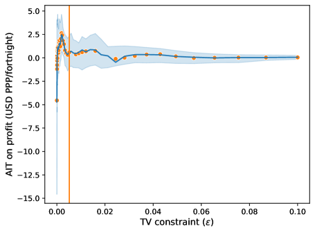
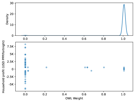
Figure 10: Estimating the Average Intent to Treat (AIT) effect on household profits in the micro-credit study Angelucci et al. (2015) in the presence of outliers. Left: the AIT estimates using OWL for various values of $\epsilon$ along with $90\%$ OS-bootstrap vertical confidence bands. The vertical line is drawn at the value $\epsilon_{0}=0.005$ obtained by the tuning procedure in Section 2.2.3, and roughly coincides with the $\epsilon$ beyond which the AIT estimates stabilize and the size of the confidence bands shrinks (see Appendix G). Right: shows that the weights estimated by OWL procedure at $\epsilon=\epsilon_{0}$ down-weight roughly $1\%$ of the households that have outlying profit values (for visual clarity, we omit a down-weighted household with profit less that $-40K$ USD PPP); see also Figure 18 in Appendix G.

8 Discussion

In this paper, we introduced the optimistically weighted likelihood (OWL) methodology, motivated by brittleness issues arising from misspecification in statistical methodology based on standard likelihoods. On the theoretical side, we established the consistency of our approach and showed its asymptotic connection to the coarsened inference methodology. We also proposed a feasible alternating optimization scheme to implement the methodology and demonstrated its empirical utility on both simulated and real data.

The OWL methodology opens up several interesting future directions. One practical open problem is how to scale to larger datasets. As a weighted likelihood method, OWL requires solving for a weight vector whose dimension is the size of the dataset. While we can solve the resulting convex optimization problem for thousands of data points, the procedure becomes significantly more complicated when the size of the dataset exceeds computer memory. How do we maintain a feasible solution, i.e. one that lies in the intersection of the simplex and some probability ball, when the entire vector cannot fit in memory?

Another practical question is how to apply the OWL approach in more complex models; for example, involving dependent data. This may be relatively straightforward for models in which the likelihood can still be written in product form due to conditional independence given random effects. This would open up its application to nested, longitudinal, spatial and temporal data, as random effects models are routinely used in such settings.

On the theoretical side, there remain important gaps to fill between our theory and practice. In particular, our theory for continuous spaces required the use of kernels to smooth our approximations to the OKL. However, in practice, we observed that generally no such smoothing is necessary, and we may simply use the finite space approximation to the OKL to achieve excellent results. Resolving this gap would have important implications for the general applicability of the OWL methodology.

Finally, a very interesting question is how to choose the corruption parameter $\epsilon\in(0,1)$ for our procedure. In our simulation study (Section 5) we chose $\epsilon$ in two ways: using the data based tuning procedure in Section 2.2.3, and using knowledge of the true corruption fraction at the population level, both of which lead to an equally robust performance. In contrast, for our application (Section 6) we explored model fit on a range of $\epsilon$ values. The population setup based on a general distance $\boldsymbol{d}$ (recall Section 2.1 focused on $\boldsymbol{d}=\text{d}_{\text{TV}}$) can provide more insights on how the choice of $\epsilon$ affects parameter inference. The OWL procedure interpolates between the maximum-likelihood estimate $\operatorname*{arg\,min}_{\theta\in\Theta}\operatorname{KL}(P_{0}|P_{\theta})$ at $\epsilon=0$ and minimum-distance estimate $\operatorname*{arg\,min}_{\theta\in\Theta}\boldsymbol{d}(P_{0},P_{\theta})$ at $\epsilon=\varepsilon_{0}$, where $\varepsilon_{0}=\min_{\theta\in\Theta}\boldsymbol{d}(P_{0},P_{\theta})$, while choosing much larger values of $\epsilon$ will eventually degrade performance. Is it possible that OWL with well-chosen $\epsilon\in[0,\varepsilon_{0}]$ can get us the best of both worlds—efficiency from the likelihood and robustness from the distance? Some of these properties can be understood by studying asymptotic properties of the parameter estimates from OWL, which is an open direction for future work.

Appendix A Properties of the OKL

This section covers some technical lemmas about the OKL function that will be used in the theoretical results in the remainder of the appendix. When showing the asymptotic connection between coarsened likelihood and OKL (Appendix D), we will allow for more general distances than the total variation (TV) distance. To this end, let $\boldsymbol{d}(P,Q)$ denote a general distance between probability measures $P,Q\in\mathcal{P}(\mathcal{X})$. We define the OKL function for a general distance $\boldsymbol{d}$ by

$$I_{\epsilon}(\theta)=\inf_{\begin{subarray}{c}Q\in\mathcal{P}(\mathcal{X})\\ \boldsymbol{d}(Q,P_{0})\leq\epsilon\end{subarray}}\operatorname{KL}(Q|P_{\theta}).$$ (11)

Although such extended analysis with general distances might be possible, for simplicity, we will restrict to the case of $\boldsymbol{d}=\text{d}_{\text{TV}}$ while proving the sandwiching property of the I-projection (Section A.2) and the consistency of the OKL estimator in continuous spaces (Appendix C).

A.1 Continuity of OKL in the coarsening radius

The following lemma shows when we can expect the OKL function to be continuous in $\epsilon$.

Lemma 2.

Let $0\leq\epsilon_{0}<\epsilon$ and $\alpha>0$. Suppose the function $Q\mapsto\boldsymbol{d}(Q,P_{0})$ is convex, then

$$0\leq I_{\epsilon}(\theta)-I_{\epsilon+\alpha}(\theta)\leq\frac{\alpha}{\epsilon-\epsilon_{0}+\alpha}I_{\epsilon_{0}}(\theta).$$

If we additionally have $\alpha\leq\epsilon-\epsilon_{0}$, then

$$0\leq I_{\epsilon-\alpha}(\theta)-I_{\epsilon}(\theta)\leq\frac{\alpha}{\epsilon-\epsilon_{0}}I_{\epsilon_{0}}(\theta).$$

Proof.

We will prove the first statement, as the second follows identically. First observe that we always have $I_{t}(\theta)-I_{t^{\prime}}(\theta)\geq 0$ for all $t^{\prime}\geq t\geq 0$. Moreover, if $I_{\epsilon_{0}}(\theta)$ is infinite, then the above holds trivially. Thus, we may assume that $I_{\epsilon_{0}}(\theta)<\infty$.

Pick $\delta>0$. By the definition of OKL, for any $r>0$ there exists $Q_{r}\in\mathcal{P}(\mathcal{X})$ such that $\boldsymbol{d}(Q_{r},P_{0})\leq r$ and

$$\operatorname{KL}(Q_{r}|P_{\theta})\leq I_{r}(\theta)+\delta.$$

Take $Q=(1-\lambda)Q_{\epsilon+\alpha}+\lambda Q_{\epsilon_{0}}\in\mathcal{P}(\mathcal{X})$ for $\lambda=\frac{\alpha}{\epsilon-\epsilon_{0}+\alpha}$. By the convexity of $\boldsymbol{d}$, we have

$$\boldsymbol{d}(Q,P_{0})\leq(1-\lambda)\boldsymbol{d}(Q_{\epsilon+\alpha},P_{0})+\lambda\boldsymbol{d}(Q_{\epsilon_{0}},P_{0})\leq(1-\lambda)(\epsilon+\alpha)+\lambda\epsilon_{0}\leq\epsilon.$$

Moreover, by the convexity of KL divergence (see e.g. [Budhiraja and Dupuis, 2019, Lemma 2.4])

$$I_{\epsilon}(\theta)\leq\operatorname{KL}(Q|P_{\theta}) \leq(1-\lambda)\operatorname{KL}(Q_{\epsilon+\alpha}|P_{\theta})+\lambda\operatorname{KL}(Q_{\epsilon_{0}}|P_{\theta})$$

$$\leq(1-\lambda)(I_{\epsilon+\alpha}(\theta)+\delta)+\lambda(I_{\epsilon_{0}}(\theta)+\delta)$$

$$\leq I_{\epsilon+\alpha}(\theta)+\frac{\alpha}{\epsilon-\epsilon_{0}+\alpha}I_{\epsilon_{0}}(\theta)+\delta.$$

Rearranging and noting that $\delta>0$ was chosen arbitrarily, gives us the result in the lemma. The second statement is derived in an identical manner by substituting $\epsilon-\alpha$ in place of $\epsilon$. ∎

A.2 Sandwiching property of I-projections

In parts of this appendix, we will be dealing with cases where $\mathcal{X}\subseteq\mathbb{R}^{d}$ and $P_{0}$ and $P_{\theta}$ have corresponding densities $p_{0},p_{\theta}\in\mathscr{D}(\mathcal{X})$ with respect to the Lebesgue measure $\lambda$. In this setting, if $I_{\epsilon}(\theta)<\infty$, then by Csiszár [1975] there is a ($\lambda$-almost everywhere) unique density $q^{*}_{\epsilon}\in\mathscr{D}(\mathcal{X})$ that we will call the information ($I$-)projection such that $\text{d}_{\text{TV}}(q^{*}_{\epsilon},p_{0})\leq\epsilon$ and $\operatorname{KL}(q^{*}_{\epsilon}|p_{\theta})=I_{\epsilon}(\theta)$. We will show that $q^{*}_{\epsilon}$ satisfies the following sandwiching property relative to $p_{0}$ and $p_{\theta}$ for any value of $\epsilon>0$.

Definition A.1.

For probability vectors $p,q,r\in\Delta_{n}$, we say that $r$ is sandwiched between $p$ and $q$ if $\min(p_{i},q_{i})\leq r_{i}\leq\max(p_{i},q_{i})$ for all $i=1,\ldots,n$. Similarly, if $p,q,r\in\mathscr{D}(\mathcal{X})$ are probability densities, then we say that $r$ is sandwiched between $p$ and $q$ if the condition $\min(p(x),q(x))\leq r(x)\leq\max(p(x),q(x))$ holds for $\lambda$-almost every $x$.

The following proposition will be important in proving the sandwiching property for the I-projection.

Proposition 2.

For probability vectors (or densities), if $r$ is sandwiched between $p$ and $q$, then $\text{d}_{\text{TV}}(r,p)\leq\text{d}_{\text{TV}}(q,p)$ and $\operatorname{KL}(r|p)\leq\operatorname{KL}(q|p)$.

In fact, will prove the above result for any $\phi$-divergence $D_{\phi}(p,q)=\int\phi(p/q)qd\lambda$ when $\phi$ is a convex function $\phi(1)=0$. The total variation distance ($\phi(x)=|x-1|$) and KL-divergence ($\phi(x)=x\log x$) will emerge as special cases.

Lemma 3.

Let $\phi:\mathbb{R}\to(-\infty,\infty]$ be a proper convex function with $\phi(1)=0$. If a density $r$ is sandwiched between densities $p$ and $q$, then $D_{\phi}(r,q)\leq D_{\phi}(p,q)$.

Proof.

The sandwiching property implies that there is a function $t:\mathcal{X}\to[0,1]$ such that $r=(1-t)p+tq$. Hence

$$D_{\phi}(r,q) =\int\phi((1-t)p/q+tq/q)qd\lambda\leq\int(1-t)\phi(p/q)qd\lambda+\int t\phi(1)qd\lambda$$

$$=D_{\phi}(p,q)-\int t\phi(p/q)qd\lambda\leq D_{\phi}(p,q)-\xi\int tq(p/q-1)d\lambda=D_{\phi}(p,q).$$

where the two inequalities follow from the convexity of $\phi$ noting that there is $\xi\in\mathbb{R}$ (called the sub-gradient) such that $\phi(x)\geq\phi(1)+\xi(x-1)=\xi(x-1)$ for all $x\in\mathbb{R}$, and the last equality holds since $\int t(p-q)d\lambda=0$, since $p$ and $r$ are assumed to integrate to one. ∎

Now, we will need a simple lemma about total variation distance before we can prove the sandwiching property of the I-projection. For brevity, we will use notations like $\{p\leq q\}$ and $\{q>\max(p_{0},p_{\theta})\}$ to denote the sets $\{x\in\mathcal{X}:p(x)\leq q(x)\}$ and $\{x\in\mathcal{X}:q(x)>\max(p_{0}(x),p_{\theta}(x))\}$ respectively. Note that for two densities $p,q\in\mathscr{D}(\mathcal{X})$, the total variation distance can be expressed as $\text{d}_{\text{TV}}(p,q)=\int_{p>q}(p-q)d\lambda=\int_{q>p}(q-p)d\lambda=\frac{1}{2}\int|p-q|d\lambda$.

Lemma 4.

Let $p,q,r\in\mathscr{D}(\mathcal{X})$. If $\{r<q\}\subseteq\{p\leq r\}$ or $\{r>q\}\subseteq\{p\geq r\}$ then $\text{d}_{\text{TV}}(p,r)\leq\text{d}_{\text{TV}}(p,q)$.

Proof.

Suppose $\{r<q\}\subseteq\{p\leq r\}$, then

$$\text{d}_{\text{TV}}(p,r)=\int_{\{p>r\}}(p-r)d\lambda\leq\int_{\{p>r\}}(p-q)d\lambda\leq\int_{\{p>q\}}(p-q)d\lambda=\text{d}_{\text{TV}}(p,q)$$

where the two inequalities follow from the inclusion $\{p>r\}\subseteq\{r\geq q\}\cap\{p>q\}$. Similarly if $\{r>q\}\subseteq\{p\geq r\}$ then,

$$\text{d}_{\text{TV}}(p,r)=\int_{\{p<r\}}(r-p)d\lambda\leq\int_{\{p<r\}}(q-p)d\lambda\leq\int_{\{p<q\}}(q-p)d\lambda=\text{d}_{\text{TV}}(p,q)$$

since $\{p<r\}\subseteq\{r\leq q\}\cap\{p<q\}$. ∎

Lemma 5.

Let $p_{0},p_{\theta}$ be probability densities satisfying $I_{\epsilon}(\theta)<\infty$, and let $q^{*}_{\epsilon}$ denote the I-projection of $p_{\theta}$ onto the set $\{q\in\mathscr{D}(\mathcal{X}):\text{d}_{\text{TV}}(q,p_{0})\leq\epsilon\}$. Then $q^{*}_{\epsilon}$ is sandwiched between $p_{0}$ and $p_{\theta}$.

Proof.

It suffices to show that for any density $q\in\mathscr{D}(\mathcal{X})$, there is a density $\bar{q}\in\mathscr{D}(\mathcal{X})$ sandwiched between $p_{0}$ and $p_{\theta}$ such that $\text{d}_{\text{TV}}(\bar{q},p_{0})\leq\text{d}_{\text{TV}}(q,p_{0})$ and $\operatorname{KL}(\bar{q}|p_{\theta})\leq\operatorname{KL}(q|p_{\theta})$. We can then complete the proof by noting that $\bar{q}=q^{*}_{\epsilon}$ if we set $q=q^{*}_{\epsilon}$.

Let $q\in\mathscr{D}(\mathcal{X})$ be given, and suppose that the set $S^{+}=\{q>\max(p_{0},p_{\theta})\}$ has non-zero Lebesgue measure. Letting

$$v=\int_{S^{+}}(q-\max(p_{0},p_{\theta}))\,d\lambda,$$

note that

$$\text{d}_{\text{TV}}(q,p_{\theta})=\int_{\{q>p_{\theta}\}}(q-p_{\theta})\,d\lambda\geq v.$$

Define the density

$$\bar{q}(x)=\begin{cases}\max(p_{0}(x),p_{\theta}(x))&\text{ if }x\in S^{+}\\ q(x)+\frac{v}{\text{d}_{\text{TV}}(q,p_{\theta})}(p_{\theta}(x)-q(x))&\text{ if }p_{\theta}(x)>q(x)\\ q(x)&\text{ otherwise }\end{cases}.$$

Then it is not hard to verify that $\bar{q}$ integrates to one and satisfies $\bar{q}(x)\leq\max(p_{0}(x),p_{\theta}(x))$ everywhere. Next, applying Lemma 4 with $p=p_{0}$, $q=q$ and $r=\bar{q}$, we obtain $\text{d}_{\text{TV}}(\bar{q},p_{0})\leq\text{d}_{\text{TV}}(q,p_{0})$ since $\{\bar{q}<q\}=S^{+}\subseteq\{p_{0}\leq\bar{q}\}$ holds. Additionally, $\bar{q}$ is sandwiched between $p_{\theta}$ and $q$. Next, Proposition 2 implies that $\operatorname{KL}(\bar{q}|p_{\theta})\leq\operatorname{KL}(q|p_{\theta})$.

Now let $q\in\mathscr{D}(\mathcal{X})$ such that $S^{+}$ is empty but the set $S^{-}=\{q<\min(p_{0},p_{\theta})\}$ is non-empty. Letting

$$v=\int_{S^{-}}(\min(p_{0},p_{\theta})-q)\,d\lambda,$$

note that $0<v\leq\text{d}_{\text{TV}}(q,p_{\theta})$, and define the density

$$\bar{q}(x)=\begin{cases}\min(p_{0}(x),p_{\theta}(x))&\text{ if }x\in S^{-}\\ q(x)+\frac{v}{\text{d}_{\text{TV}}(q,p_{\theta})}(p_{\theta}(x)-q(x))&\text{ if }p_{\theta}(x)<q(x)\\ q(x)&\text{ otherwise }\end{cases}.$$

Then observe that $\bar{q}$ is a density and it is sandwiched between $q$ and $p_{\theta}$. Similar arguments as above using Lemma 4 and Proposition 2 show that $\text{d}_{\text{TV}}(\bar{q},p_{0})\leq\text{d}_{\text{TV}}(q,p_{0})$ and $\operatorname{KL}(\bar{q}|p_{\theta})\leq\operatorname{KL}(q|p_{\theta})$. ∎

Appendix B Convergence of OKL estimator in finite spaces

In this section, we will work with a finite data space but allow for a more general distance function. To this end, let $\boldsymbol{d}(p,q)$ denote the distance between probability vectors $p,q\in\Delta_{\mathcal{X}}$. Then the OKL function for a general distance in eq. 11 translates to this setting as

$$I_{\epsilon}(\theta)=\inf_{\begin{subarray}{c}q\in{\Delta}_{\mathcal{X}}\\ \boldsymbol{d}(p,p_{0})\leq\epsilon\end{subarray}}\operatorname{KL}(q|p_{\theta}).$$ (12)

Given a dataset $x_{1},\ldots,x_{n}\in\mathcal{X}$, the finite approximation to the OKL for general distance $\boldsymbol{d}$ is given by

$$\hat{I}_{\epsilon,\textnormal{fin}}(\theta)=\inf_{\begin{subarray}{c}q\in{\Delta}_{\mathcal{X}}\\ \operatorname{supp}(q)=\hat{\mathcal{X}}_{n}\\ \boldsymbol{d}(q,\hat{p}_{\textnormal{fin}})\leq\epsilon\end{subarray}}\sum_{x\in\hat{\mathcal{X}}_{n}}q(x)\log\frac{q(x)}{p_{\theta}(x)},$$ (13)

where $\hat{\mathcal{X}}_{n}=\{x_{1},\ldots,x_{n}\}$ is the observed support and $\hat{p}_{\textnormal{fin}}(y)=\frac{|\{i\in[n]|x_{i}=y\}|}{n}$. When $\boldsymbol{d}(p,q)=\frac{1}{2}\|p-q\|_{1}$ is the total variation distance, the above is equivalent to the form given in eq. 2 as shown in the following lemma.

Lemma 6.

For any $\epsilon>0$ and $x_{1},\ldots,x_{n}\in\mathcal{X}$,

$$\inf_{\begin{subarray}{c}q\in{\Delta}_{\mathcal{X}}\\ \operatorname{supp}(q)=\hat{\mathcal{X}}_{n}\\ \frac{1}{2}\|q-\hat{p}_{\textnormal{fin}}\|_{1}\leq\epsilon\end{subarray}}\sum_{x\in\hat{\mathcal{X}}_{n}}q(x)\log\frac{q(x)}{p_{\theta}(x)}\ =\ \inf_{\begin{subarray}{c}w\in{\Delta}_{n}\\ \frac{1}{2}\|w-o\|_{1}\leq\epsilon\end{subarray}}\sum_{i=1}^{n}w_{i}\log\frac{w_{i}n\hat{p}_{\textnormal{fin}}(x_{i})}{p_{\theta}(x_{i})}.$$

where $o=(1/n,\ldots,1/n)\in\Delta_{n}$.

Proof.

For convenience, let $n_{i}=n\hat{p}_{\textnormal{fin}}(x_{i})$ and let $n(x)=n\hat{p}_{\textnormal{fin}}(x)$. For any $q\in{\Delta}_{\mathcal{X}}$ satisfying $\operatorname{supp}(q)=\hat{\mathcal{X}}_{n}$, let $w_{q}\in\Delta_{n}$ satisfy $w_{q,i}=q(x_{i})/n_{i}$. Then we have

$$\|w_{q}-o\|_{1}=\sum_{i=1}^{n}\left|\frac{q(x_{i})}{n_{i}}-\frac{1}{n}\right|=\sum_{x\in\hat{\mathcal{X}}_{n}}n(x)\left|\frac{q(x)}{n(x)}-\frac{1}{n}\right|=\|q-\hat{p}_{\textnormal{fin}}\|_{1}\text{ and }$$

$$\sum_{i=1}^{n}w_{q,i}\log\frac{w_{q,i}n_{i}}{p_{\theta}(x_{i})}=\sum_{i=1}^{n}\frac{q(x_{i})}{n_{i}}\log\frac{q(x_{i})}{p_{\theta}(x_{i})}=\sum_{x\in\hat{\mathcal{X}}_{n}}q(x)\log\frac{q(x)}{p_{\theta}(x)}.$$

The above two equalities imply that

$$\inf_{\begin{subarray}{c}q\in{\Delta}_{\mathcal{X}}\\ \operatorname{supp}(q)=\hat{\mathcal{X}}_{n}\\ \frac{1}{2}\|q-\hat{p}_{\textnormal{fin}}\|_{1}\leq\epsilon\end{subarray}}\sum_{x\in\hat{\mathcal{X}}_{n}}q(x)\log\frac{q(x)}{p_{\theta}(x)}\ \geq\ \inf_{\begin{subarray}{c}w\in{\Delta}_{n}\\ \frac{1}{2}\|w-o\|_{1}\leq\epsilon\end{subarray}}\sum_{i=1}^{n}w_{i}\log\frac{w_{i}n\hat{p}_{\textnormal{fin}}(x_{i})}{p_{\theta}(x_{i})}.$$

Now for any $w\in\Delta_{n}$, let $q_{w}\in{\Delta}_{\mathcal{X}}$ satisfy $q_{w}(x)=\sum_{i:x_{i}=x}w_{i}$. Note that we trivially must have $\operatorname{supp}(q_{w})=\hat{\mathcal{X}}_{n}$. Moreover, we have

$$\|q_{w}-\hat{p}_{\textnormal{fin}}\|_{1}=\sum_{x\in\hat{\mathcal{X}}_{n}}\left|\left(\sum_{i:x_{i}=x}w_{i}\right)-\frac{n(x)}{n}\right|\leq\sum_{x\in\hat{\mathcal{X}}_{n}}\sum_{i:x_{i}=x}\left|w_{i}-\frac{1}{n}\right|=\|w-o\|_{1}\text{ and }$$

$$\sum_{x\in\hat{\mathcal{X}}_{n}}q_{w}(x)\log\frac{q_{w}(x)}{p_{\theta}(x)}=\sum_{x\in\hat{\mathcal{X}}_{n}}\left(\sum_{i:x_{i}=x}w_{i}\right)\log\frac{\left(\sum_{i:x_{i}=x}w_{i}\right)}{p_{\theta}(x)}\leq\sum_{i=1}^{n}w_{i}\log\frac{w_{i}n_{i}}{p_{\theta}(x_{i})},$$

where the first inequality is the triangle inequality and the second inequality is the log sum inequality [Cover and Thomas, 2006, Theorem 2.7.1]. Together, the above implies that

$$\inf_{\begin{subarray}{c}q\in{\Delta}_{\mathcal{X}}\\ \operatorname{supp}(q)=\hat{\mathcal{X}}_{n}\\ \frac{1}{2}\|q-\hat{p}_{\textnormal{fin}}\|_{1}\leq\epsilon\end{subarray}}\sum_{x\in\hat{\mathcal{X}}_{n}}q(x)\log\frac{q(x)}{p_{\theta}(x)}\ \leq\ \inf_{\begin{subarray}{c}w\in{\Delta}_{n}\\ \frac{1}{2}\|w-o\|_{1}\leq\epsilon\end{subarray}}\sum_{i=1}^{n}w_{i}\log\frac{w_{i}n\hat{p}_{\textnormal{fin}}(x_{i})}{p_{\theta}(x_{i})}.\ \ \ \qed$$

To prove convergence of the estimator in eq. 13, we will make the following assumptions on the space $\mathcal{X}$ and distance $\boldsymbol{d}$.

Assumption B.1.

$\mathcal{X}$ is a finite set, $\boldsymbol{d}$ is a metric, $\boldsymbol{d}$ is jointly convex in its arguments, and there exists a constant $C\geq 1$ for which $\boldsymbol{d}(p,q)\leq C\|p-q\|_{1}$ for all $p,q\in\Delta_{\mathcal{X}}$.

Observe that Assumption B.1 fulfills the conditions of Lemma 2, implying that $I_{\epsilon}(\theta)$ is continuous in $\epsilon$. To get quantitative bounds, we make the following assumption.

Assumption B.2.

There exist constants $V,\epsilon_{0}>0$ such that $I_{\epsilon_{0}}(\theta)\leq V$.

Finally, we will also require some conditions on the support of $p_{\theta}$ and $p_{0}$.

Assumption B.3.

There exists a set $S\subseteq\mathcal{X}$ and constant $\gamma_{0}>0$ such that $\operatorname{supp}(p_{\theta})=S\subseteq\operatorname{supp}(p_{0})$ and $p_{0}(x)\geq\gamma_{0}$ for all $x\in S$.

Given the above assumptions, we have the following convergence result for $\hat{I}_{\epsilon,\textnormal{fin}}(\theta)$.

Theorem 5.

Pick $\epsilon>\epsilon_{0}$ and let $n\geq\max\left\{\frac{1}{\gamma_{0}}\log\frac{2|S|}{\delta},\frac{1}{2}\left(\frac{C|S|}{\epsilon-\epsilon_{0}}\right)^{2}\log\frac{4|S|}{\delta}\right\}$, and suppose Assumptions B.1, B.3 and B.2 hold. If $x_{1},\ldots,x_{n}\overset{i.i.d.}{\sim}p_{0}$, then with probability at least $1-\delta$,

$$|I_{\epsilon}(\theta)-\hat{I}_{\epsilon,\textnormal{fin}}(\theta)|\leq\frac{CV|S|}{\epsilon-\epsilon_{0}}\sqrt{\frac{1}{2n}\log\frac{2|S|}{\delta}}.$$

Proof.

If $n\geq\frac{1}{\gamma_{0}}\log\frac{2|S|}{\delta}$, then with probability $1-\delta/2$, we have $S\subseteq\hat{\mathcal{X}}_{n}$. Moreover, an application of Hoeffding’s inequality tells us that with probability at least $1-\delta/2$, we have

$$\|\hat{p}_{\textnormal{fin}}-p_{0}\|_{1}\leq|S|\sqrt{\frac{1}{2n}\log\frac{4|S|}{\delta}}.$$

By a union bound, both of these events occur with probability at least $1-\delta$. Condition on these two events occurring.

Now observe that any $q\in\Delta_{\mathcal{X}}$ that achieves $\operatorname{KL}_{\mathcal{X}}(q|p^{\theta})<\infty$ must satisfy $q(x)=0$ for all $x\not\in S$. Thus, we may rewrite the OKL and our finite estimator as

$$I_{\epsilon}(\theta) =\inf_{\begin{subarray}{c}q\in\Delta_{\mathcal{X}}\\ \operatorname{supp}(q)\subseteq S\\ \boldsymbol{d}(q,p_{0})\leq\epsilon\end{subarray}}\operatorname{KL}(q|p_{\theta})$$

$$\hat{I}_{\epsilon,\textnormal{fin}}(\theta) =\inf_{\begin{subarray}{c}q\in\Delta_{\mathcal{X}}\\ \operatorname{supp}(q)\subseteq\hat{\mathcal{X}}_{n}\cap S\\ \boldsymbol{d}(q,\hat{p}_{\textnormal{fin}})\leq\epsilon\end{subarray}}\operatorname{KL}(q|p_{\theta})=\inf_{\begin{subarray}{c}q\in\Delta_{\mathcal{X}}\\ \operatorname{supp}(q)\subseteq S\\ \boldsymbol{d}(q,\hat{p}_{\textnormal{fin}})\leq\epsilon\end{subarray}}\operatorname{KL}(q|p_{\theta}),$$

where we have used the fact that we are conditioning on $S\subseteq\hat{\mathcal{X}}_{n}$.

Moreover, by Assumption B.1 and our bound on $\|\hat{p}_{\textnormal{fin}}-p_{0}\|_{1}$, we have:

$$\boldsymbol{d}(q,\hat{p}_{\textnormal{fin}})\leq\boldsymbol{d}(q,p_{0})+\boldsymbol{d}(\hat{p}_{\textnormal{fin}},p_{0})\leq\boldsymbol{d}(q,p_{0})+C\|\hat{p}_{\textnormal{fin}}-p_{0}\|_{1}\leq\boldsymbol{d}(q,p_{0})+\alpha_{n},$$

where $\alpha_{n}=C|S|\sqrt{\frac{1}{2n}\log\frac{2|S|}{\delta}}$. Similarly, we also can conclude $\boldsymbol{d}(q,\hat{p}_{\textnormal{fin}})\geq\boldsymbol{d}(q,p_{0})-\alpha_{n}.$

Applying Lemma 2, we have

$$\hat{I}_{\epsilon,\textnormal{fin}}(\theta) =\inf_{\begin{subarray}{c}q\in\Delta_{\mathcal{X}}\\ \operatorname{supp}(q)\subseteq S\\ \boldsymbol{d}(q,\hat{p}_{\textnormal{fin}})\leq\epsilon\end{subarray}}\operatorname{KL}(q|p_{\theta})\geq\inf_{\begin{subarray}{c}q\in\Delta_{\mathcal{X}}\\ \operatorname{supp}(q)\subseteq S\\ \boldsymbol{d}(q,p_{0})\leq\epsilon+\alpha\end{subarray}}\operatorname{KL}(q|p_{\theta})$$

$$=I_{\epsilon+\alpha_{n}}(\theta)\geq I_{\epsilon}(\theta)-\frac{\alpha_{n}}{\epsilon-\epsilon_{0}+\alpha_{n}}V.$$

On the other hand, if $n\geq\frac{1}{2}\left(\frac{C|S|}{\epsilon-\epsilon_{0}}\right)^{2}\log\frac{4|S|}{\delta}$, then $\alpha_{n}\leq\epsilon-\epsilon_{0}$, and we can again apply Lemma 2 to see that

$$\hat{I}_{\epsilon,\textnormal{fin}}(\theta) =\inf_{\begin{subarray}{c}q\in\Delta_{\mathcal{X}}\\ \operatorname{supp}(q)\subseteq S\\ \boldsymbol{d}(q,\hat{p}_{\textnormal{fin}})\leq\epsilon\end{subarray}}\operatorname{KL}(q|p_{\theta})\leq\inf_{\begin{subarray}{c}q\in\Delta_{\mathcal{X}}\\ \operatorname{supp}(q)\subseteq S\\ \boldsymbol{d}(q,p_{0})\leq\epsilon-\alpha\end{subarray}}\operatorname{KL}(q|p_{\theta})$$

$$=I_{\epsilon-\alpha_{n}}(\theta)\leq I_{\epsilon}(\theta)+\frac{\alpha_{n}}{\epsilon-\epsilon_{0}}V.$$

Rearranging the above inequalities gives us the lemma statement. ∎

Appendix C Convergence of OKL estimator in Euclidean spaces

In this section, we show consistency (and convergence rates) for the OKL estimator when $\mathcal{X}=\mathbb{R}^{d}$ is the Euclidean space. To avoid technical complications with tail estimation, we will restrict our analysis to the case when both the data and the model family are supported on a compact set $S\subseteq\mathcal{X}$. The results and notation in this section are self-contained, and can be read independently of other sections.

C.1 Introduction

Consider the data space $\mathcal{X}=\mathbb{R}^{d}$ equipped with the Euclidean norm $\|\cdot\|$ and its Borel sigma algebra $\mathcal{B}$. We will let $\mathscr{D}(\mathcal{X})=\{f:\mathcal{X}\to[0,\infty)\mid\int f(x)dx=1,f\text{ is $\mathcal{B}$-measurable}\}$ denote the set of densities on $\mathcal{X}$ with respect to the Lebesgue measure $\lambda$. Given the data density $p_{0}\in\mathscr{D}(\mathcal{X})$, model family $\{p_{\theta}\}_{\theta\in\Theta}\subseteq\mathscr{D}(\mathcal{X})$ and coarsening radius $\epsilon>0$, the central object of interest in this section is the OKL function defined as

$$I_{\epsilon}(\theta)=\inf_{\begin{subarray}{c}q\in\mathscr{D}(\mathcal{X})\\ \text{d}_{\text{TV}}(q,p_{0})\leq\epsilon\end{subarray}}\operatorname{KL}(q|p_{\theta}),$$ (14)

where, given two densities $p,q\in\mathscr{D}(\mathcal{X})$, the total variation distance between them is $\text{d}_{\text{TV}}(q,p)=\frac{1}{2}\int|q(x)-p(x)|dx$, and the KL-divergence is $\operatorname{KL}(p|q)=\int p(x)\log\frac{p(x)}{q(x)}dx$ if the absolute continuity condition $\int p(x)I\{q(x)=0\}dx=0$ is satisfied, otherwise $\operatorname{KL}(p|q)=\infty$.

Given samples $x_{1},\ldots,x_{n}\in\mathcal{X}$ drawn i.i.d. from the distribution with density $p_{0}$, and a suitable kernel $K_{h}:\mathcal{X}\times\mathcal{X}\to\mathbb{R}$, we will approximate $I_{\epsilon}(\theta)$ with the value of a finite-dimensional optimization problem given by

$$\hat{I}_{\epsilon}(\theta)=\inf_{\begin{subarray}{c}w\in\hat{\Delta}_{n}\\ \frac{1}{2}\|w-o\|_{1}\leq\epsilon\end{subarray}}\sum_{i=1}^{n}w_{i}\log\frac{nw_{i}\hat{p}(x_{i})}{p_{\theta}(x_{i})},$$ (15)

where $\hat{p}$ is a suitable density estimator for $p_{0}$, $\Delta_{n}=\{(v_{1},\ldots,v_{n})|\sum_{i=1}^{n}v_{i}=1,v_{i}\geq 0\}$ is the $n$-dimensional probability simplex, $o=(1/n,\ldots,1/n)\in\Delta_{n}$ is the constant probability vector, $A$ is an $n\times n$ matrix with entries $A_{ij}=\frac{K_{h}(x_{i},x_{j})}{n\hat{p}(x_{i})}$, $\hat{\Delta}_{n}=A\Delta_{n}$ is the image of the set $\Delta_{n}\subseteq\mathbb{R}^{n}_{+}$ under the linear operator $A$, and $\|(x_{1},\ldots,x_{d})\|_{1}=\sum_{i=1}^{d}|x_{i}|$ is the $\ell_{1}$ norm of the vector.

C.1.1 Assumptions and statement of the result

To describe the formal statement quantifying the approximation between eq. 14 and eq. 15, we will introduce a series of assumptions. Our result will handle the case when densities $p_{0}$ and $p_{\theta}$ are smooth densities supported on a bounded set $S\subseteq\mathcal{X}$ whose boundary has measure zero, i.e. $\lambda(S\setminus S^{\circ})=0$, where $S^{\circ}$ denotes the interior of $S$. We fix a value $\theta\in\Theta$ throughout this section.

Assumption C.1.

Suppose $S\subseteq\mathcal{X}$ is a subset of the closed unit ball $\bar{B}(0,R)$ of radius $R$, with finite Lebesgue measure $V_{S}=\lambda(S)\geq 1$, and has a boundary measure functional $\phi(r)=\frac{\lambda(S\setminus S_{-r})}{\lambda(S)}$ that satisfies $\lim_{r\rightarrow 0}\phi(r)=0$.

Here $S_{-r}=\{x\in S:B(x,r)\subseteq S\}$ denotes the set of points for which the unit ball of radius $B(x,r)=\{y\in\mathcal{X}|\|x-y\|\leq r\}$ is also contained inside $S$. For example, when $S=B(x_{0},r_{0})$ is the unit ball of radius $r_{0}$ centered at the point $x_{0}$, the boundary measure functional is given by

$$\phi(r)=1-\frac{\lambda(B(x,r_{0}-r))}{\lambda(B(x,r_{0}))}=1-\left(1-\frac{r}{r_{0}}\right)^{d}$$

since $S_{-r}=B(x_{0},r_{0}-r)$.

Next we have the following smoothness and support condition on densities $p_{0},p_{\theta}\in\mathscr{D}(\mathcal{X})$. Here the support of a density $p\in\mathscr{D}(\mathcal{X})$ is defined as $\operatorname{supp}(p)=\{x\in\mathcal{X}:p(x)>0\}$.

Assumption C.2.

The supports satisfy $\operatorname{supp}(p_{0})=\operatorname{supp}(p_{\theta})=S$, and there exists $\gamma\in(0,1]$ such that $p_{0}(x),p_{\theta}(x)\in[\gamma,1/\gamma]$ for all $x\in S$.

Assumption C.3.

$p_{0}$ and $\log p_{\theta}$ are $\alpha$-Hölder smooth on $S$. More precisely, there are constants $\alpha,C_{\alpha}>0$ such that $|p_{0}(x)-p_{0}(y)|,|\log p_{\theta}(x)-\log p_{\theta}(y)|\leq C_{\alpha}\|x-y\|^{\alpha}$ for all $x,y\in S$.

Finally, we will require the following assumption on the kernel $K_{h}:\mathcal{X}\times\mathcal{X}\to\mathbb{R}$.

Assumption C.4.

The kernel satisfies $K_{h}(x,y)=\frac{1}{h^{d}}\kappa\left(\frac{\|x-y\|_{2}}{h}\right)$ for a non-increasing continuous function $\kappa:\mathbb{R}_{+}\rightarrow\mathbb{R}_{+}$ satisfying (i) $\int_{\mathbb{R}^{d}}\kappa(\|x\|_{2})\,dx=1$, (ii) $\kappa(0)\leq c_{0}$ for some fixed constant $c_{0}>0$, and (iii) there exist constants $t_{0},C_{\rho},\rho$ such that $\rho\leq 1$ and $t_{0}\geq 1$ so that for all $t>t_{0}$, $k(t)\leq C_{\rho}\exp(-t^{\rho})$. Further, suppose that (iv) for every $h>0$, the kernel $K_{h}$ is a positive semi-definite kernel, i.e. the $m\times m$ matrix $(K_{h}(y_{i},y_{j}))_{i,j\in[m]}$ for any $y_{1},\ldots,y_{m}\in\mathbb{R}^{d}$ and $m\geq 1$ is positive semi-definite.

Parts (i)-(iii) in Assumption C.4 are standard assumptions in the kernel density estimation literature (see, e.g. Jiang [2017]), while part (iv) allows us to use techniques from reproducing kernel Hilbert spaces. By Shoenberg’s theorem (see e.g. Ressel [1976]) part (iv) of Assumption C.4 is satisfied whenever $\kappa$ is a completely monotone function (see e.g. Merkle [2014]). In particular, note that Assumption C.4 is satisfied by the Gaussian kernel given as $\kappa(t)=\frac{1}{(2\pi)^{d/2}}\exp(-t^{2})$.

Definition C.1.

Suppose Assumption C.4 holds and observations $x_{1},\ldots,x_{n}\overset{i.i.d.}{\sim}p_{0}$ are given. Define a mapping $L:\Delta_{n}\mapsto\mathscr{D}(\mathcal{X})$ from the $n$-dimensional probability simplex $\Delta_{n}$ to the space of densities $\mathscr{D}(\mathcal{X})$ given by $L(w)=\hat{q}_{w}$, where

$$\hat{q}_{w}(\cdot)=\sum_{i=1}^{n}w_{i}K_{h}(\cdot,x_{i}).$$

For the probability density estimator $\hat{p}$ in the Monte Carlo estimate of the objective in eq. 14, we use the kernel density estimate $\hat{p}=\hat{q}_{o}$, where $o=(1/n,\ldots,1/n)\in\Delta_{n}$.

Using the parameterization $w=Av$ for $v\in\Delta_{n}$, one can rewrite eq. 15 using the above notation as:

$$\hat{I}_{\epsilon}(\theta)=\inf_{\begin{subarray}{c}v\in\Delta_{n}\\ \frac{1}{2n}\sum_{i=1}^{n}\left|\frac{\hat{q}_{v}(x_{i})}{\hat{p}(x_{i})}-1\right|\leq\epsilon\end{subarray}}\frac{1}{n}\sum_{i=1}^{n}\frac{\hat{q}_{v}(x_{i})}{\hat{p}(x_{i})}\log\frac{\hat{q}_{v}(x_{i})}{p_{\theta}(x_{i})}.$$

In order to ensure stability of the optimization objective in eq. 15 and guarantee regularity in the optimal weights, we will restrict the optimization over weights that do not deviate too far from uniformity and replace $\hat{p}$ by the ‘clipped’ version of our estimator: $\hat{p}_{\gamma}(x)=\min(\max(\hat{p}(x),\gamma),1/\gamma)$. To that end, define $\Delta_{n}^{r}=\{v\in\Delta_{n}:n\cdot v_{i}\in[r,1/r]\text{ for all }i\}$ for $r\leq 1$. Then for our theoretical result, we will consider a version of the estimator

$$\hat{I}_{\epsilon}(\theta)=\inf_{\begin{subarray}{c}v\in\Delta_{n}^{\gamma^{2}/4}\\ \frac{1}{2n}\sum_{i=1}^{n}\left|\frac{\hat{q}_{v}(x_{i})}{\hat{p}_{\gamma}(x_{i})}-1\right|\leq\epsilon\end{subarray}}\frac{1}{n}\sum_{i=1}^{n}\frac{\hat{q}_{v}(x_{i})}{\hat{p}_{\gamma}(x_{i})}\log\frac{\hat{q}_{v}(x_{i})}{p_{\theta}(x_{i})},$$ (16)

where $\gamma$ is the value from Assumption C.2.

Under the above assumptions, we have the following result:

Theorem 6.

Suppose Assumptions C.1, C.2, C.3 and C.4 hold and $n\geq n_{0},h\leq\bar{h},and\frac{\log n}{\sqrt{n}h^{d}}\leq\bar{\eta}$ for suitable constants $\bar{h},n_{0},\bar{\eta}>0$ that depend on the quantities in the assumptions. Fix a $\beta>0$, and suppose we obtain an i.i.d. sample $x_{1},\ldots,x_{n}$ of size $n$ from density $p_{0}$. Then with probability at least $1-e^{-(\log n)^{2\beta}}$,

$$\left|\hat{I}_{\epsilon}(\theta)-I_{\epsilon}(\theta)\right|\leq O\left(\frac{\log n}{\sqrt{n}h^{d}}+h^{\min(\alpha/2,1)}\log\frac{1}{h}+\phi(\sqrt{h})\log\frac{1}{\phi(\sqrt{h})}\right),$$

where the $O(\cdot)$ hides constant factors depending on the quantities in Assumptions C.1-C.4, and on the choice of $\epsilon,\beta>0$.

When $S=B(0,R)$ is a Euclidean ball of radius $R$, Taylor expansion shows that $\phi(\sqrt{h})=\frac{\sqrt{h}d}{R}+O(h)$. Suppose, for simplicity that $\alpha\geq 1$, then taking $h=n^{-\frac{1}{2d+1}}$ and $\beta=1$, we see that $|\hat{I}_{\epsilon}(\theta)-I_{\epsilon}(\theta)|=\tilde{O}(n^{-\frac{1}{4d+2}})$ upto a logarithmic factor in $n$, with probability at least $1-1/n$.

Note that the choice of bandwidth parameter $h=o(n^{-\frac{1}{2d}})$ required to shrink our error terms to zero decreases more slowly with $n$ than the optimal rate $h=o(n^{-1/d})$ for density estimation [Rigollet and Vert, 2009]. This suggests that our error bounds can potentially be improved. Note also that the above result holds for any fixed value of $\theta\in\Theta$; extensions to uniform convergence over all $\theta\in\Theta$ may be possible with further assumptions on the complexity of the class $\Theta$ and continuity of the map $\theta\mapsto\log p_{\theta}(\cdot)$, but we do not pursue this direction here.

Proof outline of Theorem 6.

We sketch the proof here.

Section C.3.1

First, Lemma 12 shows that with high probability for large $n$, the estimators of KL divergence and total variation in eq. 16 are close to their population counterparts $\operatorname{KL}(\hat{q}_{v}|p_{\theta})$ and $\text{d}_{\text{TV}}(\hat{q}_{v},p_{0})$ for any $v\in\Delta_{n}$ such that $\hat{q}_{v}$ is suitably bounded. See Corollary 3 for the most useful version of this statement.

Section C.3.2

Next, Lemma 17 shows that for any density $q$ over $S$ satisfying Assumption C.2, with high probability for large $n$, there exists a $v\in\Delta_{n}^{\gamma}$ such that $\hat{q}_{v}$ is a pointwise accurate estimator of $K_{h}\star q$, where $K_{h}\star q$ denotes the convolution of the density $q$ with the probability kernel $K_{h}$. Combined with Lemma 5, which establishes the boundedness of the minimizer $q^{*}_{\epsilon}$ in eq. 14, we have that there exists a pointwise accurate estimator $\hat{q}_{v^{*}}$ of $K_{h}\star q^{*}_{\epsilon}$ for some $v^{*}\in\Delta_{n}^{\gamma^{2}/4}$.

Section C.3.3

Lemma 18 shows that under Assumption C.3, $\operatorname{KL}(K_{h}\star q|p_{\theta})$ and $\text{d}_{\text{TV}}(K_{h}\star q,p_{0})$ must not be much greater than $\operatorname{KL}(q|p_{\theta})$ and $\text{d}_{\text{TV}}(q,p_{0})$, respectively, when $h$ is sufficiently small.

We combine the above arguments (see Section C.4), to show that the optimal objective value in eq. 14 corresponding to the minimizer $q^{*}_{\epsilon}$, must be close to the optimal objective value in eq. 16, thus showing that $\hat{I}_{\epsilon}(\theta)$ can well approximate $I_{\epsilon}(\theta)$ when $h$ is small, and $n$ is large. ∎

While Section C.3 covers the main steps of proof, there are useful results in Section C.2 that provide upper bounds on the tail probability and second moment of the kernel $K_{h}$ based on Assumption C.4. These results are used in Section C.3.3 and Section C.4.

Additional notation

For $p\in\mathscr{D}(\mathcal{X})$ and $A\subseteq\mathcal{X}$, we will use the shorthand $p(A)$ to denote the quantity $\int_{A}p(x)dx$. For a probability density kernel $K_{h}$, let

$$\widetilde{p}_{h}(\cdot)=(K_{h}\star p)(\cdot)=\int p(y)K_{h}(\cdot,y)dy\in\mathscr{D}(\mathcal{X})$$

denote the kernel-smoothed version of a density $p\in\mathscr{D}(\mathcal{X})$. Similarly, for a measure $\mu$ on $\mathcal{X}$, we can define $(K_{h}\star\mu)(x)=\int K_{h}(x,y)\mu(dy)$. For a set $S\subseteq\mathbb{R}^{d}$ and $p,q\in\mathscr{D}(\mathcal{X})$, let $\operatorname{KL}_{S}(q|p)=\int_{S}q(x)\log\frac{p(x)}{q(x)}\,dx$. The constant $v_{d}$ will denote the volume of the Euclidean ball in $\mathbb{R}^{d}$. The notation $\|f\|_{1}=\int|f(x)|dx$ and $\|f\|_{\infty}=\sup_{x\in\mathcal{X}}|f(x)|$ will denote the $L_{1}$ and $L_{\infty}$ norm of the function $f$. For $p,q\in\mathscr{D}(\mathcal{X})$, recall that $\text{d}_{\text{TV}}(p,q)=\frac{1}{2}\|p-q\|_{1}.$

C.2 Kernel tail bounds

In this sub-section, we derive tail bounds for a class of probability kernels $K_{h}(x,y)=\frac{1}{h^{d}}\kappa(\|x-y\|/h)$ on $\mathbb{R}^{d}$ indexed by parameter $h>0$ used for density estimation, when the function $\kappa:[0,\infty)\to[0,\infty)$ has exponentially decaying tails (see parts (i)-(iii) of Assumption C.4). The following two lemmas bound the tail distribution and the variance of the random variable $Z$ having density $x\mapsto\kappa(\|x\|)$. These results will then be used to obtain tails bounds for the kernel $K_{h}$.

Lemma 7.

Suppose Assumption C.4 holds. If $Z$ is an $\mathbb{R}^{d}$ valued random vector with probability density $x\mapsto\kappa(\|x\|)$, then

$$\mathbb{P}(\|Z\|\geq t)=\int_{\|x\|\geq t}\kappa(\|x\|)dx\leq C_{1}t^{d+1-\rho}e^{-t^{\rho}}$$ (17)

for each $t\geq t_{1}=\max(\Gamma(a+1)^{1/{\rho(a-1)}},t_{0})\geq 1$ where $\Gamma$ is the Gamma function, $a=\frac{d+1}{\rho}$, and $C_{1}>0$ is a constant depending on constants $t_{0},C_{\rho},\rho>0$ in Assumption C.4 and dimension $d$. Explicitly, $C_{1}=\rho^{-1}C_{\rho}v_{d}2^{a-1}$, where $v_{d}=\frac{\pi^{d/2}}{\Gamma(d/2+1)}$ is the volume of the unit ball in $\mathbb{R}^{d}$.

Proof.

Using [Jiang, 2017, Lemma 4] and the upper bound on tails of $\kappa$ since $s\geq t\geq t_{0}$,

$$\int_{\|x\|\geq t}\kappa(\|x\|)dx=v_{d}\int_{t}^{\infty}\kappa(r)r^{d}dr\leq C_{\rho}v_{d}\int_{t}^{\infty}e^{-r^{\rho}}r^{d}dr.$$

Using the substitution $s=r^{\rho}$, we obtain

$$\int_{t}^{\infty}e^{-r^{\rho}}r^{d}dr=\frac{1}{\rho}\int_{t^{\rho}}^{\infty}e^{-s}s^{\frac{d+1}{\rho}-1}ds=\frac{1}{\rho}\Gamma\left(a,t^{\rho}\right)$$

where $\Gamma(a,y)=\int_{y}^{\infty}e^{-x}x^{a-1}dx$ is the incomplete Gamma function and $a=\frac{d+1}{\rho}\geq 2$. Taking $b_{a}=\Gamma(a+1)^{1/(a-1)}$, we have the following bound on the incomplete Gamma function [Pinelis, 2020, Theorem 1.1] for $a\geq 2$:

$$\Gamma(a,y)\leq\frac{((b_{a}+y)^{a}-y^{a})e^{-y}}{ab_{a}}=\frac{e^{-y}\int_{0}^{b_{a}}a(x+y)^{a-1}dx}{ab_{a}}\leq(b_{a}+y)^{a-1}e^{-y}.$$

Since $t^{\rho}\geq b_{a}$, the proof can be completed by combining the above displays along with the bound

$$\Gamma(a,t^{\rho})\leq 2^{a-1}t^{\rho(a-1)}e^{-t^{\rho}}=2^{a-1}t^{d+1-\rho}e^{-t^{\rho}}.$$

∎

Lemma 8.

Suppose Assumption C.4 holds. If $Z$ is an $\mathbb{R}^{d}$ valued random vector with probability density $x\mapsto\kappa(\|x\|)$, then

$$\mathbb{E}_{Z}[\|Z\|_{2}^{2}]\leq v_{d}\left(c_{0}t_{0}^{d+3}+\frac{C_{\rho}}{\rho}\Gamma\left(\frac{d+3}{\rho}\right)\right),$$

where $v_{d}$ is the volume of the unit ball in $d$-dimensions and $\Gamma(\cdot)$ is the Gamma function.

Proof.

We can write

$$\mathbb{E}_{Z}[\|Z\|_{2}^{2}]=\int_{\mathbb{R}^{d}}\|z\|_{2}^{2}\kappa(\|z\|_{2})\,dz=v_{d}\int_{0}^{\infty}\kappa(t)t^{d+2}\,du,$$

where the second equality follows from [Jiang, 2017, Lemma 4]. Taking $c_{0},t_{0},\rho,C_{\rho}$ as the constants from Assumption C.4, we have

$$\int_{0}^{\infty}\kappa(t)t^{d+2}\,du =\int_{0}^{t_{0}}\kappa(t)t^{d+2}\,du+\int_{t_{0}}^{\infty}\kappa(t)t^{d+2}\,du$$

$$\leq c_{0}t_{0}^{d+3}+C_{\rho}\int_{t_{0}}^{\infty}\exp(-t^{\rho})t^{d+2}\,du$$

$$\leq c_{0}t_{0}^{d+3}+\frac{C_{\rho}}{\rho}\int_{0}^{\infty}\exp(-u)u^{\frac{d+3}{\rho}-1}\,du$$

$$=c_{0}t_{0}^{d+3}+\frac{C_{\rho}}{\rho}\Gamma\left(\frac{d+3}{\rho}\right),$$

where we have used the substitution $u=t^{\rho}$ in the second inequality as well as the fact that the integrands are non-negative from 0 to $\infty$, and the last line follows from the definition of the Gamma function. ∎

We now use the above lemmas to prove properties about the kernel $K_{h}$.

Lemma 9.

Suppose that Assumption C.4 holds. For any $x\in\mathbb{R}^{d}$,

$$\int_{B(x,r)}K_{h}(x,y)\,dy\geq 1-\frac{C_{1}k!}{(r/h)^{4}}$$

whenever $r\geq t_{1}h$, where $B(x,r)$ denotes the open ball of radius $r$ around $x$, constants $C_{1},t_{1}>0$ are as defined in Lemma 7, and $k=\lceil\frac{5+d}{\rho}\rceil-1$. In particular, for any bounded set $S\subset\mathbb{R}^{d}$ and any $x\in S$, we have

$$\int_{S}K_{h}(x,y)\,dy\geq 1-\frac{C_{1}k!}{(r_{x}/h)^{4}}$$

whenever $r_{x}\geq t_{1}h$, where $r_{x}=\inf_{y\in S^{c}}\|x-y\|_{2}$. If $0<h\leq h_{0}=\min(\frac{1}{C_{1}k!},\frac{1}{t_{1}^{2}})$, we can always take $r=\sqrt{h}$, and the bound on the right hand side simplifies to $1-\frac{C_{1}k!}{(r/h)^{4}}\geq 1-h$.

Proof.

Let $Z$ be an $\mathbb{R}^{d}$-valued random vector with probability density $z\mapsto\kappa(\|z\|_{2})$, then

$$1-\int_{B(x,r)}K_{h}(x,y)\,dy =\Pr(x+hZ\notin B(x,r))$$

$$=\Pr\left(\|Z\|_{2}\geq\frac{r}{h}\right)\leq C_{1}(r/h)^{(d+1-\rho)}e^{-(r/h)^{\rho}}$$

$$\leq\frac{C_{1}k!}{(r/h)^{k\rho-(d+1-\rho)}}\leq\frac{C_{1}k!}{(r/h)^{4}}.$$

where the inequality in the second line follows from Lemma 7 whenever $r\geq t_{1}h$, and the inequality on the last line follows by using $e^{y}\geq\frac{y^{k}}{k!}$ and $k\rho-(d+1-\rho)\geq 4$. To get the statement for set $S$, we observe that $1-\int_{S}K_{h}(x,y)\,dy\geq 1-\int_{B(x,r_{x})}K_{h}(x,y)\,dy$.

∎

For any probability measure $\mu$ on $\mathcal{X}$, we define the density $f_{h,\mu}(y)=\int K_{h}(y,x)\mu(dx)\in\mathscr{D}(\mathcal{X})$ obtained by convolving $\mu$ with the kernel $K_{h}$. The next result bounds the TV-distance $\text{d}_{\text{TV}}(f_{h,\mu},f_{h,\nu})$ in terms of the supremum norm $\|f_{h,\mu}-f_{h,\nu}\|_{\infty}$ when measures $\mu$ and $\nu$ are supported on $S$.

Corollary 1.

Suppose Assumptions C.2 and C.4 hold and $\mu$ and $\nu$ are two probability measures supported on $S$. Then whenever $h\leq 1/t_{1}$,

$$\text{d}_{\text{TV}}(f_{h,\mu},f_{h,\nu})\leq\frac{v_{d}(R+1)^{d}}{2}\|f_{h,\mu}-f_{h,\nu}\|_{\infty}+C_{1}h^{d+1-\rho}{e^{-h^{-1/\rho}}}$$

where $v_{d}$ is the volume of the unit ball in $\mathbb{R}^{d}$, and $t_{1}$ is as defined in Lemma 7.

Proof.

We first claim that

$$\int_{\|y\|\geq R+1}f_{h,\mu}(y)dy\leq C_{1}(1/h)^{d+1-\rho}e^{-(1/h)^{\rho}}\text{ for any $h\leq 1/t_{1}$}.$$ (18)

To see this, we note that $f_{h,\mu}(y)=\int_{S}K_{h}(x,y)\mu(dx)$, since $\mu$ is supported on $S$ and $K_{h}$ is symmetric. Thus by Fubini’s theorem

$$\int_{\|y\|\geq R+r}f_{h,\mu}(y)dy=\int_{S}\left(\int_{\|y\|\geq R+r}K_{h}(x,y)dy\right)\mu(dx).$$

Next, note that the proof of Lemma 9 shows that

$$\int_{\|y\|\geq R+1}K_{h}(x,y)dy\leq 1-\int_{B(x,1)}K_{h}(x,y)dy\leq C_{1}(1/h)^{d+1-\rho}e^{-(1/h)^{\rho}}$$

for any $x\in S$ since $B(x,1)\subseteq B(0,R+1)$ whenever $x\in S\subseteq B(0,R)$, proving eq. 18.

To finish the proof of the lemma, observe that

$$\text{d}_{\text{TV}}(f_{h,\mu},f_{h,\nu}) =\frac{1}{2}\int_{B(0,R+1)}|f_{h,\mu}(x)-f_{h,\nu}(x)|dx+\frac{1}{2}\int_{\|x\|\geq R+1}|f_{h,\mu}(x)-f_{h,\nu}(x)|dx$$

$$\leq\frac{v_{d}}{2}(R+1)^{d}\|f_{h,\mu}-f_{h,\nu}\|_{\infty}+C_{1}h^{d+1-\rho}{e^{-h^{-1/\rho}}}$$

where the bound on the second term follows from eq. 18. ∎

Next, we can see how well the convolved density $\widetilde{q}_{h}=(K_{h}\star q)\in\mathscr{D}(\mathcal{X})$ approximates the density $q\in\mathscr{D}(\mathcal{X})$. For instance, if the density $q$ is supported on a bounded set $S\subseteq\mathbb{R}^{d}$ with non-zero Lebesgue measure $V_{S}$, with boundary functional $\phi(r)=\frac{\lambda(S\setminus S_{-r})}{\lambda(S)}$ (see Assumption C.1), then the following Lemma provides an upper bound on the mass placed by the convolved density $\widetilde{q}_{h}$ outside the set $S$.

Lemma 10.

Suppose that Assumption C.1 and Assumption C.4 hold. For any probability density $q\in\mathscr{D}(\mathcal{X})$ and density bounded above by $1/\gamma$ and supported on the set $S$,

$$\widetilde{q}_{h}(S^{c})\doteq\int_{S^{c}}\widetilde{q}_{h}(x)dx\leq h+\frac{V_{S}}{\gamma}\phi(\sqrt{h})$$

whenever $h\leq h_{0}$, where $h_{0}$ is as given in Lemma 9.

Proof.

We use the following chain of arguments:

$$\widetilde{q}_{h}(S^{c}) =\int_{S^{c}}\widetilde{q}_{h}(x)dx=\int_{S^{c}}\int_{S}q(y)K_{h}(x,y)dydx$$

$$=\int_{S}q(y)\int_{S^{c}}K_{h}(x,y)\,dx\,dy$$

$$=\int_{S_{-\sqrt{h}}}q(y)\int_{S^{c}}K_{h}(x,y)\,dx\,dy+\int_{S\setminus S_{-\sqrt{h}}}q(y)\int_{S^{c}}K_{h}(x,y)\,dx\,dy$$

$$\leq h+\int_{S\setminus S_{-\sqrt{h}}}q(y)\,dy\leq h+\frac{V_{S}}{\gamma}\phi(\sqrt{h}),$$

where the first inequality uses $\int_{S^{c}}K_{h}(x,y)dx=1-\int_{S}K_{h}(y,x)dx$ is bounded above by $h$ if $y\in S_{-\sqrt{h}}$ (Lemma 9) or by one if $y\in S\setminus S_{-\sqrt{h}}$, and the second inequality holds from the definition of boundary functional $\phi$ and the upper bound on the density $q$. ∎

For a set $S\subseteq\mathbb{R}^{d}$, let $\operatorname{KL}_{S}(q|p)=\int_{S}q(x)\log\frac{p(x)}{q(x)}\,dx$. The following lemma provides a useful trick to translate between $\operatorname{KL}$ and $\text{d}_{\text{TV}}$ expressions for densities that are not supported on $S$ to densities that are supported on $S$.

Lemma 11.

Suppose $q\in\mathscr{D}(\mathcal{X})$ is a density that may not be supported on $S$. Then there is a density $\bar{q}$ supported on $S$ such that

$$\operatorname{KL}_{S}(q|p_{\theta})=(1-q(S^{c}))(\operatorname{KL}(\bar{q}|p_{\theta})+\log(1-q(S^{c})))$$

and $\text{d}_{\text{TV}}(\bar{q},p_{0})\leq\text{d}_{\text{TV}}(q,p_{0})+q(S^{c}).$

Proof.

We will take $\bar{q}(x)=\frac{q(x)}{q(S)}I\{x\in S\}$ to be the restriction of the density $q$ to $S$. It is straightforward to see that the equality for the KL terms hold. The TV bound follows from the triangle inequality, noting that $\text{d}_{\text{TV}}(\bar{q},q)=\frac{1}{2}\int_{\mathbb{R}^{d}}\lvert\bar{q}(x)-q(x)\rvert dx=q(S^{c})$. ∎

C.3 Proof of Theorem 1

C.3.1 Uniform convergence of KL and TV estimators

The main result of this subsection is the following.

Lemma 12.

There exists an absolute constant $c_{1}>0$ such that the following holds. Suppose observations $x_{1},\ldots,x_{n}$ are drawn i.i.d. from $p_{0}$, and that Assumption C.2 and Assumption C.4 hold. Let $\hat{q}_{w}$ be as defined in Definition C.1. Let $\hat{p}=\hat{q}_{o}$, where $o=(1/n,\ldots,1/n)\in\Delta_{n}$, be the kernel-density estimator for $p_{0}$ based on observations $x_{1},\ldots x_{n}$, and let $\hat{p}_{\gamma}(\cdot)=\min(\max(\hat{p}(\cdot),\gamma),1/\gamma)$ be its truncated version. With probability at least $1-\delta$, we have

$$\left|\left(\|\hat{q}_{w}-p_{0}\|_{1}-\hat{q}_{w}(S^{c})\right)-\frac{1}{n}\sum_{i=1}^{n}\left|\frac{\hat{q}_{w}(x_{i})}{\hat{p}_{\gamma}(x_{i})}-1\right|\right| \leq\frac{c_{1}u}{\gamma^{3}}\left(\frac{c_{0}}{\sqrt{n}h^{d}}+\sqrt{\frac{2}{n}\log\frac{6}{\delta}}+\text{d}_{\text{TV}}(\hat{p},p_{0})\right)\hskip 10.00002pt\text{ and }$$

$$\left|\operatorname{KL}_{S}(\hat{q}_{w}|p_{\theta})-\frac{1}{n}\sum_{i=1}^{n}\frac{\hat{q}_{w}(x_{i})}{\hat{p}_{\gamma}(x_{i})}\log\frac{\hat{q}_{w}(x_{i})}{p_{\theta}(x_{i})}\right| \leq\left(\frac{c_{1}u}{\gamma^{3}}\log\frac{u}{\ell\gamma}\right)\left(\frac{c_{0}}{\sqrt{n}h^{d}}+\sqrt{\frac{2}{n}\log\frac{6}{\delta}}+\text{d}_{\text{TV}}(\hat{p},p_{0})\right).$$

uniformly over all $w\in\mathcal{W}_{\ell,u}=\{w\in\Delta_{n}\,:\,\hat{q}_{w}(x_{i})\in[\ell,u]\text{ for all }i\in[n]\}$, where thresholds $u,l$ are chosen so that $u\geq\max(1,\gamma e)\geq 1\geq\ell$ and $\|f\|_{1}=\int|f(x)|dx$.

To establish this result, we will use techniques from uniform law of large numbers over a class of functions $\mathscr{F}\subseteq\{f:S\rightarrow\mathbb{R}\}$. For a fixed class $\mathscr{F}$, given i.i.d. samples $x_{1},\ldots,x_{n}$ from density $p_{0}$ supported on $S\subseteq\mathcal{X}$, we consider the empirical Rademacher complexity (e.g. Boucheron et al. [2005]) of the function class $\mathscr{F}$ defined as:

$$\mathcal{R}_{n}(\mathscr{F})=\mathbb{E}_{\epsilon}\left[\sup_{f\in\mathscr{F}}\left|\frac{1}{n}\sum_{i=1}^{n}\epsilon_{i}f(x_{i})\right|\right]$$ (19)

where the expectation is over Rademacher random variables $\epsilon_{1},\ldots\epsilon_{n}\overset{i.i.d.}{\sim}\operatorname{Uniform}(\{-1,1\})$. The Rademacher complexity is a measure of richness of a function class that can be used to obtain a uniform law of large numbers result like the following standard result.

Lemma 13 (c.f. Theorem 3.2 of [Boucheron et al., 2005]).

Let $\mathscr{F}\subset\{f:S\rightarrow[-a,a]\}$ be a fixed class of bounded functions and suppose $\delta>0$. If $x_{1},\ldots,x_{n}\sim p_{0}$, then with probability at least $1-\delta$

$$\sup_{f\in\mathscr{F}}\left|\frac{1}{n}\sum_{i=1}^{n}f(x_{i})-\int f(x)p_{0}(x)dx\right|\leq 2\mathcal{R}_{n}(\mathscr{F})+a\sqrt{\frac{2}{n}\log\frac{2}{\delta}}.$$

Thus a typical task to obtain uniform laws of large numbers is to obtain upper bounds on $\mathcal{R}_{n}(\mathscr{F})$ for various function classes $\mathscr{F}$. To this end, the following results will be useful:

Lemma 14 (c.f. Theorem 3.3 of [Boucheron et al., 2005]).

Suppose $g:S\rightarrow\mathbb{R}$ is a bounded function, $\mathscr{F}\subset\{f:S\rightarrow\mathbb{R}\}$, and $\psi:\mathbb{R}\rightarrow\mathbb{R}$ is a function with Lipschitz constant $L$. Then

$$\mathcal{R}_{n}(\{x\mapsto g(x)f(x):f\in\mathscr{F}\}) \leq\mathcal{R}_{n}(\mathscr{F})\sup_{x\in S}|g(x)|$$

$$\mathcal{R}_{n}(\{x\mapsto\psi(f(x)):f\in\mathscr{F}\}) \leq L\mathcal{R}_{n}(\mathscr{F})+\frac{|\psi(0)|}{\sqrt{n}}.$$

Proof.

The above statements with $\psi(0)=0$ follow from Theorem 3.3 of [Boucheron et al., 2005]. To handle the case $\psi(0)\neq 0$, define $\tilde{\psi}=\psi-\psi(0)\boldsymbol{1}$ where $\boldsymbol{1}$ denotes the function taking the constant value one, and note that

$$\mathcal{R}_{n}(\{\psi\circ f:f\in\mathscr{F}\}) =\mathcal{R}_{n}(\{\tilde{\psi}\circ f+\psi(0)\boldsymbol{1}:f\in\mathscr{F}\})$$

$$=\mathcal{R}_{n}(\{\tilde{\psi}\circ f:f\in\mathscr{F}\})+\mathcal{R}_{n}(\{\psi(0)\boldsymbol{1}\})$$

$$\leq L\mathcal{R}_{n}(\mathscr{F})+|\psi(0)|\mathcal{R}_{n}(\boldsymbol{1})$$

where we have used that $\mathcal{R}_{n}(\{\boldsymbol{1}\})\leq\mathbb{E}_{\epsilon}\lvert\frac{1}{n}\sum_{i=1}^{n}\epsilon_{i}\rvert\leq\sqrt{\mathbb{E}_{\epsilon}\left(\frac{1}{n}\sum_{i=1}^{n}\epsilon_{i}\right)^{2}}=n^{-1/2}.$ ∎

Lemma 15 (Lemma 22 of [Bartlett and Mendelson, 2002]).

Let $k:\mathcal{X}\times\mathcal{X}\rightarrow\mathbb{R}$ be a positive definite kernel satisfying $k(x,x)\leq c$ for all $x\in\mathcal{X}$. Then, for the function class

$$\mathscr{F}_{a}=\bigg{\{}\cdot\mapsto\sum_{i=1}^{m}w_{i}k(\cdot,y_{i})\,:\,m\geq 1,y_{i}\in\mathcal{X},w_{i}\in\mathbb{R},\text{ and }\sum_{i,j}w_{i}w_{j}k(y_{i},y_{j})\leq a^{2}\bigg{\}},$$

we have $\mathcal{R}_{n}(\mathscr{F}_{a})\leq 2a\sqrt{\frac{c}{n}}$.

We will now use the above results to bound the Monte Carlo estimation error uniformly over functions generated from a data-dependent function family $\{\hat{q}_{w}:w\in\Delta_{n}\}$.

Lemma 16.

Suppose bounded functions $\alpha,\beta,\eta:S\to\mathbb{R}$ and a Lipschitz function $\Phi:\mathbb{R}\to[-M,M]$ with Lipschitz constant $L$ are given, and suppose that Assumption C.4 holds. Given a function $q:S\to\mathbb{R}$, denote $\psi(q,x)=\eta(x)\Phi(\alpha(x)q(x)+\beta(x))$. Then for any $\delta\in(0,2/e)$, with probability $1-\delta$ it holds that:

$$\sup_{w\in\Delta_{n}}\left\lvert\frac{1}{n}\sum_{i=1}^{n}\psi(\hat{q}_{w},x_{i})-\int\psi(\hat{q}_{w},x)p_{0}(x)dx\right\rvert\leq\frac{C_{1}}{h^{d}\sqrt{n}}+C_{2}\sqrt{\frac{2}{n}\log\frac{2}{\delta}}$$

where $\hat{q}_{w}$ is as in Definition C.1, $C_{1}=4\|\eta\|_{\infty}\|\alpha\|_{\infty}Lc_{0}$, and $C_{2}=\sqrt{2}\|\eta\|_{\infty}(L\|\beta\|_{\infty}+|\Phi(0)|)+\|\eta\|_{\infty}M$.

Proof.

Using $\hat{\mathcal{Q}}$ to denote the data dependent class of functions $\{\hat{q}_{w}\mid w\in\Delta_{n}\}$, and taking $\kappa=K_{h}$, $c=c_{0}/h^{d}$, and $a=\sqrt{c}$ in Lemma 15, let us first note that $\hat{\mathcal{Q}}\subseteq\mathscr{F}_{a}$. Indeed, this holds since for any $w=(w_{1},\ldots,w_{n})\in\Delta_{n}$ we have $\hat{q}_{w}(\cdot)=\sum_{i=1}^{n}K_{h}(\cdot,x_{i})w_{i}$ and

$$\sum_{i,j=1}^{n}w_{i}w_{j}K_{h}(x_{i},x_{j})\leq c\sum_{i=1}^{n}\sum_{j=1}^{n}w_{i}w_{j}=c,$$

where the inequality follows from the Cauchy Schwarz bound $K_{h}(x,y)\leq\sqrt{K_{h}(x,x)K_{h}(y,y)}$ using the positive definiteness of the kernel $K_{h}$, and the bound $K_{h}(x,x)\leq c_{0}/h^{d}=c$ from Assumption C.4. Further, note by Lemma 15 that $\mathcal{R}_{n}(\mathscr{F}_{a})\leq\frac{2c_{0}}{h^{d}\sqrt{n}}$.

Next, let $\mathscr{G}$ denote the fixed function class $\{x\mapsto\psi(f,x)|f\in\mathscr{F}_{a}\}$. Repeated application of Lemma 14 shows:

$$\mathcal{R}_{n}(\mathscr{G}) \leq\|\eta\|_{\infty}\|\alpha\|_{\infty}L\mathcal{R}_{n}(\mathscr{F}_{a})+\frac{\|\eta\|_{\infty}(L\|\beta\|_{\infty}+|\Phi(0)|)}{\sqrt{n}}$$

$$\leq\frac{2\|\eta\|_{\infty}\|\alpha\|_{\infty}Lc_{0}}{h^{d}\sqrt{n}}+\frac{\|\eta\|_{\infty}(L\|\beta\|_{\infty}+|\Phi(0)|)}{\sqrt{n}}.$$

Thus we can complete the proof by an application of Lemma 13 for the bounded class of functions $\mathscr{F}=\mathscr{G}$, and noting the inclusion $\hat{\mathcal{Q}}\subseteq\mathscr{F}_{a}$. ∎

With these uniform convergence results in place, now we can prove the main result of this section:

Proof of Lemma 12.

By assumption

$$\frac{1}{n}\sum_{i=1}^{n}\left|\frac{1}{p_{0}(x_{i})}-\frac{1}{\hat{p}_{\gamma}(x_{i})}\right|\leq\frac{1}{\gamma^{2}n}\sum_{i=1}^{n}\left|p_{0}(x_{i})-\hat{p}_{\gamma}(x_{i})\right|\leq\frac{1}{\gamma^{2}n}\sum_{i=1}^{n}(\left|p_{0}(x_{i})-\hat{p}(x_{i})\right|\wedge\gamma^{-1}),$$

where the last inequality uses the fact that $\lvert p_{0}(\cdot)-\hat{p}_{\gamma}(\cdot)\rvert\leq\min(1/\gamma,\lvert p_{0}(\cdot)-\hat{p}(\cdot)\rvert)$ since $p_{0}(\cdot),\hat{p}_{\gamma}(\cdot)\in[1/\gamma,\gamma]$. Recall $\hat{p}=\hat{q}_{o}$, and hence we may apply Lemma 16 with $\Phi(x)=|x|\wedge\gamma^{-1}$, $\beta=p_{0}$, $\alpha(\cdot)=\eta(\cdot)=1$, and $w=o$, to show with probability $1-\delta/3$:

$$\frac{1}{n}\sum_{i=1}^{n}\left|p_{0}(x_{i})-\hat{p}(x_{i})\right|\wedge\gamma^{-1} \leq\int(\gamma^{-1}\wedge|p_{0}(x)-\hat{p}(x)|)p_{0}(x)dx+\left(\frac{4c_{0}}{h^{d}\sqrt{n}}+\frac{3}{\gamma}\sqrt{\frac{2}{n}\log\frac{6}{\delta}}\right)$$

$$\leq\frac{2}{\gamma}\text{d}_{\text{TV}}(\hat{p},p_{0})+\left(\frac{4c_{0}}{h^{d}\sqrt{n}}+\frac{3}{\gamma}\sqrt{\frac{2}{n}\log\frac{6}{\delta}}\right)=\frac{\nu}{\gamma},$$

where $\nu=2\text{d}_{\text{TV}}(\hat{p},p_{0})+\frac{4\gamma c_{0}}{h^{d}\sqrt{n}}+3\sqrt{\frac{2}{n}\log\frac{6}{\delta}}$.

Turning to the $\ell_{1}$-bound, for any $w\in\mathcal{W}_{\gamma}$, we have

$$\left|\frac{1}{n}\sum_{i=1}^{n}\left|\frac{\hat{q}_{w}(x_{i})}{\hat{p}_{\gamma}(x_{i})}-1\right|-\frac{1}{n}\sum_{i=1}^{n}\left|\frac{\hat{q}_{w}(x_{i})}{{p}_{0}(x_{i})}-1\right|\right| \leq\frac{1}{n}\sum_{i=1}^{n}\left|\left|\frac{\hat{q}_{w}(x_{i})}{\hat{p}_{\gamma}(x_{i})}-1\right|-\left|\frac{\hat{q}_{w}(x_{i})}{{p}_{0}(x_{i})}-1\right|\right|$$

$$\leq\frac{1}{n}\sum_{i=1}^{n}\left|\frac{\hat{q}_{w}(x_{i})}{\hat{p}_{\gamma}(x_{i})}-\frac{\hat{q}_{w}(x_{i})}{{p}_{0}(x_{i})}\right|\leq\frac{\nu u}{\gamma^{3}}.$$

Here the first inequality follows from the triangle inequality, the second follows from the reverse triangle inequality, and the last follows from the upper bound on $\hat{q}_{w}$ and the bounds at the beginning of the proof. Observe that $\int\lvert\frac{q(x)}{{p_{0}}(x)}-1\rvert p_{0}(x)dx=\|q-p_{0}\|_{1}-q(S^{c})$ for any density $q\in\mathscr{D}(\mathcal{X})$. Next, we apply Lemma 16 with $\Phi(x)=|x|\wedge M$, $M=u/\gamma$, $\alpha=1/p_{0}$, $\beta=-1$, $\eta=1$, noting that:

$$\psi(\hat{q}_{w},\cdot)=\left\lvert\frac{\hat{q}_{w}(\cdot)}{p_{0}(\cdot)}-1\right\rvert\wedge M=\left\lvert\frac{\hat{q}_{w}(\cdot)}{p_{0}(\cdot)}-1\right\rvert$$

for each $w\in\mathcal{W}_{\ell,u}$. Thus we have

$$\left|\frac{1}{n}\sum_{i=1}^{n}\left|\frac{\hat{q}_{w}(x_{i})}{{p_{0}}(x_{i})}-1\right|-\|\hat{q}_{w}-p_{0}\|_{1}-\hat{q}_{w}(S^{c})\right|\leq\frac{4c_{0}}{\gamma\sqrt{n}h^{d}}+\left(3+\frac{u}{\gamma}\right)\sqrt{\frac{2}{n}\log\frac{6}{\delta}},$$

with probability at least $1-\delta/3$ for all $w\in\mathcal{W}_{\ell,u}$ simultaneously.

Turning to the KL-bound, a similar chain of reasoning gives us

$$\left|\frac{1}{n}\sum_{i=1}^{n}\frac{q_{w}(x_{i})}{\hat{p}(x_{i})}\log\frac{q_{w}(x_{i})}{p_{\theta}(x_{i})}-\frac{1}{n}\sum_{i=1}^{n}\frac{q_{w}(x_{i})}{p_{0}(x_{i})}\log\frac{q_{w}(x_{i})}{p_{\theta}(x_{i})}\right|\leq\frac{\nu u}{\gamma^{3}}\log\frac{u}{\gamma},$$

where we have additionally used the lower bound $p_{\theta}(\cdot)\in[\gamma,1/\gamma]$. Next, we will invoke Lemma 16 with $\alpha=1/p_{\theta},\beta=0,\eta=p_{\theta}/p_{0}$ and $\Phi(x)=k(x)\log k(x)$ where $k(x)=\min(\max(x,u/\gamma),l\gamma)$, noting that the function $\Phi$ is bounded within radius $M=\frac{u}{\gamma}\log\frac{u}{\gamma}$ and is a Lipschitz function with Lipschitz constant bounded by $L=\sup_{x\in[l\gamma,u/\gamma]}|1+\log x|\leq 2\log\frac{u}{l\gamma}$. Then, using the bounds $C_{1}\leq\tilde{C}_{1}=\frac{8c_{0}}{\gamma^{3}}\log\frac{u}{l\gamma}$ and $C_{2}\leq\tilde{C}_{2}=\frac{3u}{\gamma^{3}}\log\frac{u}{\gamma}$, Lemma 16 shows that with probability $1-\delta/3$,

$$\left\lvert\frac{1}{n}\sum_{i=1}^{n}\frac{\hat{q}_{w}(x_{i})}{p_{0}(x_{i})}\log\frac{\hat{q}_{w}(x_{i})}{p_{\theta}(x_{i})}-\operatorname{KL}_{S}(\hat{q}_{w}|p_{\theta})\right\rvert\leq\frac{\tilde{C_{1}}}{\sqrt{n}h^{d}}+\tilde{C_{2}}\sqrt{\frac{2}{n}\log\frac{6}{\delta}}$$

for each $w\in\mathcal{W}_{\ell,u}$ simultaneously, since $\psi(\hat{q}_{w},\cdot)=\frac{\hat{q}_{w}(\cdot)}{p_{0}(\cdot)}\log\frac{\hat{q}_{w}(\cdot)}{p_{\theta}(\cdot)}$ and $\operatorname{KL}_{S}(\hat{q}_{w}|p_{\theta})=$
$\int\psi(\hat{q}_{w},x)p_{0}(x)dx$ whenever $w\in\mathcal{W}_{\ell,u}$. Finally, we obtain the lemma statement by using the union bound and putting all the display equations together, noting that $u/\gamma\geq e$ and $\gamma\leq 1$. ∎

C.3.2 Sup-norm approximation of kernel density estimates

Recall our notation for the truncated probability simplex $\Delta_{n}^{\beta}=\{(w_{1},\ldots,w_{n})\in\Delta_{n}:\frac{\beta}{n}\leq w_{i}\leq\frac{1}{n\beta}\}$. The next lemma provides approximation results for the subset of densities $\{\hat{q}_{w}:w\in\Delta_{n}^{\gamma^{2}/4}\}\subseteq\mathscr{D}(\mathcal{X})$ that hold with arbitrary high probability when $n$ is large enough. In particular, Item 1 shows that $\hat{p}$ approximates well the convolved density $K_{h}\star p_{0}$, Item 2 provides upper and lower bounds on the density $\hat{q}_{w}$, Item 3 bounds the mass of $\hat{q}_{w}$ outside the set $S$, and Item 4 shows that any convolved density of the form $K_{h}\star q$ can be approximated well by a density of the form $\hat{q}_{w}$, whenever $q(\cdot)\in[\gamma,1/\gamma]$ is a density supported on $S$.

Lemma 17.

Suppose that Assumption C.2 and Assumption C.4 hold and $\delta\in(0,1)$ is such that $n\geq\frac{2}{\gamma^{4}}\log\frac{12}{\delta}$. Further suppose that $q\in\mathscr{D}(\mathcal{X})$ is a density supported on $S$ satisfying $\gamma\leq q(x)\leq 1/\gamma$ for each $x\in S$. If $x_{1},\ldots,x_{n}\sim p_{0}$, with probability $1-\delta$, the following items hold:

1. $\|\hat{p}-K_{h}\star p_{0}\|_{\infty}\leq\frac{6c_{0}}{\sqrt{n}h^{d}}\sqrt{\log\frac{6}{\delta}}$.

2. $\frac{\gamma^{2}}{4}\left(\gamma-\frac{6c_{0}}{\sqrt{n}h^{d}}\sqrt{\log\frac{2}{\delta}}\right)\leq\hat{q}_{w}(x)\leq\frac{4}{\gamma^{2}}\left(\gamma^{-1}+\frac{6c_{0}}{\sqrt{n}h^{d}}\sqrt{\log\frac{2}{\delta}}\right)$ uniformly over $w\in\Delta_{n}^{\gamma^{2}/2}$ and $x\in\mathbb{R}^{d}$.

3. $\hat{q}_{w}(S^{c})\leq\frac{4}{\gamma^{2}}\left(h+\frac{V_{S}}{\gamma}\phi(\sqrt{h})+\sqrt{\frac{1}{2n}\log\frac{3}{\delta}}\right)$ uniformly over $w\in\Delta_{n}^{\gamma^{2}/2}$, whenever $h\leq h_{0}$, where $h_{0}$ is as defined in Lemma 9.

4. Denote $\widetilde{q}_{h}=K_{h}\star q$. There is a $w\in\Delta_{n}^{\gamma^{2}/2}$ such that $\|\hat{q}_{w}-\widetilde{q}_{h}\|_{\infty}\leq\frac{8c_{0}}{\gamma^{4}h^{d}}\sqrt{\frac{1}{n}\log\frac{12}{\delta}}$. In particular,

   $$\lvert\operatorname{KL}_{S}(\hat{q}_{w}|p_{\theta})-\operatorname{KL}_{S}(\widetilde{q}_{h}|p_{\theta})\rvert\leq\frac{C}{h^{d}\sqrt{n}}\sqrt{\log\frac{12}{\delta}}$$

   where $C=\frac{8c_{0}}{\gamma^{4}}V_{S}(1+\log(\frac{u}{\gamma l}))$ and $u$ and $l$ are the upper and lower bounds on $\hat{q}_{w}$ in Item 2. We take $C=\infty$ if $l\leq 0.$

Proof of Lemma 17.

Combining Lemma 13 with Lemma 15 shows that with probability $1-\delta/3$:

$$\left|\frac{1}{n}\sum_{i=1}^{n}K_{h}(x_{i},x)-\int K_{h}(y,x)p_{0}(y)dy\right| \leq\frac{4c_{0}}{\sqrt{n}h^{d}}+\frac{c_{0}}{\sqrt{n}h^{d}}\sqrt{2\log\frac{6}{\delta}}\leq\frac{6c_{0}}{\sqrt{n}h^{d}}\sqrt{\log\frac{6}{\delta}}.$$

for all $x\in\mathbb{R}^{d}$ simultaneously. Noting that $\hat{p}(x)=\frac{1}{n}\sum_{i}K_{h}(x_{i},x)$ and $(K_{h}\star p_{0})(x)=\int K_{h}(y,x)p_{0}(y)dy$, the uniform bound in Item 1 follows.

To show Item 2, note for each $w\in\Delta_{n}^{\gamma^{2}/4}$ that

$$\frac{\gamma^{2}\hat{p}(x)}{4}\leq\hat{q}_{w}(x)=\sum_{i=1}^{n}w_{i}K_{h}(x_{i},x)\leq\frac{4\hat{p}(x)}{\gamma^{2}}\quad\text{for each }x\in\mathbb{R}^{d}.$$

Item 2 now follows from the bound in Item 1 and as $(K_{h}\star p_{0})(\cdot)\in[\gamma,1/\gamma]$, since $\int K_{h}(y,x)dy=1$ and $p_{0}(\cdot)\in[\gamma,1/\gamma]$.

Now we will show Item 3. For arbitrary $w\in\Delta_{n}^{\gamma^{2}/4}$ observe that

$$\hat{q}_{w}(S^{c})\leq\frac{4\hat{p}(S^{c})}{\gamma^{2}}.$$

An application of Hoeffding’s inequality to the function $f(\cdot)=\int_{S^{c}}K_{h}(\cdot,x)dx\in[0,1]$ implies that with probability $1-\delta/3$,

$$\hat{p}(S^{c})=\frac{1}{n}\sum_{i=1}^{n}f(x_{i})\,dx \leq\int f(y)p_{0}(y)dydx+\sqrt{\frac{1}{2n}\log\frac{3}{\delta}}$$

$$=\int_{S^{c}}\int K_{h}(y,x)p_{0}(y)dydx+\sqrt{\frac{1}{2n}\log\frac{3}{\delta}}$$

$$\leq h+\frac{V_{S}}{\gamma}\phi(\sqrt{h})+\sqrt{\frac{1}{2n}\log\frac{3}{\delta}},$$

where, the second inequality follows by invoking Lemma 10 with the choice $q=p_{0}$ whenever $h\leq h_{0}$.

Finally to show Item 4, we choose the weights $w_{i}=\frac{q(x_{i})}{Zp_{0}(x_{i})}$ for $i=1,\ldots,n$, where $Z=\sum_{i=1}^{n}\frac{q(x_{i})}{p_{0}(x_{i})}$. By Hoeffding’s inequality, we have that with probability at least $1-\delta/6$,

$$|Z-n|=|Z-\mathbb{E}[Z]|\leq\frac{1}{\gamma^{2}}\sqrt{\frac{n}{2}\log\frac{12}{\delta}}.$$

In the event that this holds, if $n\geq\frac{2}{\gamma^{4}}\log\frac{12}{\delta}$, then $Z\in[n/2,3n/2]$ and we have that $w\in\Delta_{n}^{\gamma^{2}/4}$. Moreover, it implies that for any $x\in\mathbb{R}^{d}$,

$$\left|\hat{q}_{w}(x)-\frac{1}{n}\sum_{i=1}^{n}\frac{q(x_{i})}{p_{0}(x_{i})}K_{h}(x_{i},x)\right| =\left|\sum_{i=1}^{n}w_{i}K_{h}(x_{i},x)-\frac{1}{n}\sum_{i=1}^{n}\frac{q(x_{i})}{p_{0}(x_{i})}K_{h}(x_{i},x)\right|$$

$$\leq\left|\frac{n-Z}{Z}\right|\max_{i\in[n]}\frac{q(x_{i})}{p_{0}(x_{i})}K_{h}(x_{i},x)$$

$$\leq\frac{2}{n}|n-Z|\frac{c_{0}}{\gamma^{2}h^{d}}\leq\frac{2c_{0}}{\gamma^{4}h^{d}}\sqrt{\frac{1}{n}\log\frac{12}{\delta}}.$$

Next, observe that Lemma 14 and Lemma 15 imply that the Rademacher complexity $\mathcal{R}_{n}$ of the function class $\{\cdot\mapsto\frac{q(\cdot)}{p_{0}(\cdot)}K_{h}(\cdot,x)\,:\,x\in\mathbb{R}^{d}\}$ on domain $S$ is bounded above by $\frac{2c_{0}}{\gamma^{2}h^{d}\sqrt{n}}$. Therefore by Lemma 13, with probability $1-\delta/6$, we have

$$\sup_{x\in\mathbb{R}^{d}}\left|\frac{1}{n}\sum_{i=1}^{n}\frac{q(x_{i})}{p_{0}(x_{i})}K_{h}(x_{i},x)-\int_{S}\frac{q(y)}{p_{0}(y)}K_{h}(y,x)\,p_{0}(y)dy\right|\leq\frac{c_{0}}{\gamma^{2}h^{d}\sqrt{n}}\left(4+\sqrt{2\log\frac{12}{\delta}}\right).$$

Since $p_{0},q$ are both supported on $S$ with $\inf_{x\in S}p_{0}(x)>0$, we have $(K_{h}\star q)(x)=\int_{S}q(y)K_{h}(x,y)\,dy=\int_{S}\frac{q(y)}{p_{0}(y)}K_{h}(x,y)p_{0}(y)dy$. Hence combining the previous two display equations and using the union bound, the uniform bound in Item 4 between $\hat{q}_{w}$ and $\widetilde{q}_{h}$ is seen to hold with probability $1-\delta/3$. Finally to bound the differences between the KL terms, note that

$$\lvert\operatorname{KL}_{S}(\hat{q}_{w}|p_{\theta})-\operatorname{KL}_{S}(\widetilde{q}_{h}|p_{\theta})\rvert \leq\int_{S}|\hat{q}_{w}(x)\log\hat{q}_{w}(x)-\widetilde{q}_{h}(x)\log\widetilde{q}_{h}(x)|dx$$

$$\quad+\int_{S}|\log p_{\theta}(x)||\hat{q}_{w}(x)-\widetilde{q}_{h}(x)|dx$$

$$\leq\|\hat{q}_{w}-\widetilde{q}_{h}\|_{\infty}V_{S}(1+\log\frac{u}{\gamma l}),$$

where the last inequality follows by using the Lipschitz continuity of the map $\Phi(x)=x\log x$ on the interval $[l,u]$, with Lipschitz constants $1+\log(u/l)$, and using the upper bound $|\log p_{\theta}(\cdot)|\leq\log(1/\gamma)$.

A final application of the union bound shows that Items 1 through 4 can be simultaneously satisfied with probability $1-\delta$. ∎

C.3.3 KL and TV approximation by kernel smoothed densities

In this section we show that the terms $\operatorname{KL}(q|p_{\theta})$ and $\text{d}_{\text{TV}}(q,p_{0})$ do not increase by much when a density $q\in\mathscr{D}(\mathcal{X})$ is replaced by its kernel-smoothed version $\widetilde{q}_{h}=K_{h}\star q$ for a suitably small bandwidth parameter $h>0$.

Lemma 18.

Suppose Assumptions C.1, C.2, C.3 and C.4 hold. There exists a constant $\tilde{c}>0$ and $\tilde{h}>0$ depending only on the constants in the above assumption, such that the following statement holds. Suppose that $q\in\mathscr{D}(\mathcal{X})$ is supported on $S$ and bounded above by $1/\gamma$ and $h\leq\tilde{h}$ then

• $\text{d}_{\text{TV}}(\widetilde{q}_{h},p_{0})\leq\text{d}_{\text{TV}}(q,p_{0})+\tilde{c}\left(h^{\alpha/2}+h+\phi(\sqrt{h})\right)$

• $\operatorname{KL}_{S}(\widetilde{q}_{h}|p_{\theta})\leq\operatorname{KL}(q|p_{\theta})+\tilde{c}\left(h^{\alpha/2}+h\log\frac{1}{h}+\phi(\sqrt{h})\log\frac{1}{\phi(\sqrt{h})}\right)$.

We will prove the TV and KL statements separately. We start with the TV statement.

Lemma 19.

Suppose that $q\in\mathscr{D}(\mathcal{X})$ is supported on $S$ and suppose that Assumptions C.1, C.2, C.3 and C.4 hold. Then

$$\text{d}_{\text{TV}}(\widetilde{q}_{h},p_{0})\leq\text{d}_{\text{TV}}(q,p_{0})+V_{S}\left(C_{\alpha}h^{\alpha/2}+h+\frac{\phi(\sqrt{h})}{\gamma}\right)$$

whenever $h\in(0,h_{0})$.

Proof.

We first observe that for any densities $p,q\in\mathscr{D}(\mathcal{X})$, we have

$$\text{d}_{\text{TV}}(\widetilde{p}_{h},\widetilde{q}_{h}) =\frac{1}{2}\int_{\mathbb{R}^{d}}|\mathbb{E}_{Z\sim K}[q(x-hZ)-p(x-hZ)]|\,dx$$

$$\leq\frac{1}{2}\mathbb{E}_{Z\sim K}\int_{\mathbb{R}^{d}}|q(x-hZ)-p(x-hZ)|\,dx$$

$$=\frac{1}{2}\int_{\mathbb{R}^{d}}|q(x)-p(x)|\,dx=\text{d}_{\text{TV}}(p,q),$$

where $Z$ is an $\mathbb{R}^{d}$-valued random vector with probability density $x\mapsto\kappa(\|x\|_{2})$, and the inequality follows from Jensen’s inequality and Fubini’s theorem. By the triangle inequality, we then have

$$\text{d}_{\text{TV}}(\widetilde{q}_{h},p_{0})\leq\text{d}_{\text{TV}}(\widetilde{q}_{h},K_{h}\star p_{0})+\text{d}_{\text{TV}}(K_{h}\star p_{0},p_{0})\leq\text{d}_{\text{TV}}(q,p_{0})+\text{d}_{\text{TV}}(K_{h}\star p_{0},p_{0}).$$

Next, note that for any $x\in S_{-\sqrt{h}}$ we have

$$\left|p_{0}(x)-K_{h}\star p_{0}(x)\right|$$

$$=\left|\int_{\mathbb{R}^{d}}p_{0}(x)K_{h}(x,y)\,dy-\int_{\mathbb{R}^{d}}p_{0}(y)K_{h}(x,y)\,dy\right|$$

$$\leq\int_{\mathbb{R}^{d}}\left|p_{0}(x)-p_{0}(y)\right|K_{h}(x,y)\,dy$$

$$=\int_{B(x,\sqrt{h})}\left|p_{0}(x)-p_{0}(y)\right|K_{h}(x,y)\,dy+\int_{B(x,\sqrt{h})^{c}}\left|p_{0}(x)-p_{0}(y)\right|K_{h}(x,y)\,dy$$

$$\leq C_{\alpha}h^{\alpha/2}+h,$$

where the first inequality follows from Jensen’s inequality, and the second follows from Assumption C.3 and Lemma 9, using the upper bound on the density $p_{0}(\cdot)\leq 1/\gamma$.

Thus we have

$$\text{d}_{\text{TV}}(K_{h}\star p_{0},p_{0})$$

$$=\frac{1}{2}\int_{\mathbb{R}^{d}}\left|p_{0}(x)-K_{h}\star p_{0}(x)\right|\,dx$$

$$=\frac{1}{2}\int_{S_{-\sqrt{h}}}\left|p_{0}(x)-K_{h}\star p_{0}(x)\right|\,dx+\frac{1}{2}\int_{\mathbb{R}^{d}\setminus S_{-\sqrt{h}}}\left|p_{0}(x)-K_{h}\star p_{0}(x)\right|\,dx$$

$$\leq\frac{\lambda(S_{-\sqrt{h}})}{2}\left(C_{\alpha}h^{\alpha/2}+h\right)+\frac{1}{2}\int_{S\setminus S_{-\sqrt{h}}}\left|p_{0}(x)-(K_{h}\star p_{0})(x)\right|\,dx+\frac{1}{2}(K_{h}\star p_{0})(S^{c})$$

$$\leq V_{S}(C_{\alpha}h^{\alpha/2}+h+\gamma^{-1}\phi(\sqrt{h})).$$

where the first inequality follows from the last display equation and using the fact that $p_{0}(x)=0$ whenever $x\in S^{c}$, and the second inequality follows by using that $|p_{0}(\cdot)-(K_{h}\star p_{0})(\cdot)|\leq 1/\gamma$ and $\lambda(S\setminus S_{-r})=V_{S}\phi(r)$, along with the bound $(K_{h}\star p_{0})(S^{c})\leq h+\frac{V_{S}}{\gamma}\phi(\sqrt{h})$ from Lemma 10. ∎

We now turn to proving the KL bound. To do so, we will use the decomposition of the KL into negative entropy and cross-entropy and bound each term separately.

Lemma 20.

Suppose Assumptions C.1 and C.4 hold, $q\in\mathscr{D}(\mathcal{X})$ has support $S$ and is bounded above by $1/\gamma$. Then

$$\int_{S}\widetilde{q}_{h}(x)\log\widetilde{q}_{h}(x)dx\leq\int_{S}q(x)\log q(x)dx+D(h)\left[\frac{d}{2}\log(2\pi eM)+\left(\frac{d}{2}+1\right)\log\frac{1}{D(h)}\right],$$

where $M=2R^{2}+2v_{d}\left(c_{0}t_{0}^{d+3}+\frac{C_{\rho}}{\rho}\Gamma\left(\frac{d+3}{\rho}\right)\right)$ and $D(h)=h+\frac{V_{S}}{\gamma}\phi(\sqrt{h})$, whenever $h\leq\min(h_{0},h_{1})$ where $h_{1}=\inf\{h>0:D(h)>1/e\}.$

Proof.

First let us note that the integrals $\int_{\mathbb{R}^{d}}q(x)\log q(x)dx$ and $\int_{\mathbb{R}^{d}}\widetilde{q}_{h}(x)\log\widetilde{q}_{h}(x)dx$ are well-defined. Indeed, the first integral is well defined since $q$ is bounded above by $1/\gamma$ on a set $S$ with finite Lebesgue measure. Although, $\widetilde{q}_{h}$ can also be shown to be bounded above by $1/\gamma$, its support is unbounded if the kernel $K_{h}$ also has unbounded support. Instead, for the existence of the second integral, it suffices to show that the second moment of $\widetilde{q}_{h}$ is finite (e.g. see Ghourchian et al. [2017]). To show the latter, we will use the property a random variable $Y$ with density $\widetilde{q}_{h}$, has the same distribution as $X+hZ$, where $X$ is random variable with density $q$, and let $Z$ be a random variable with density $x\mapsto\kappa(\|x\|_{2})$ independent of $X$. Hence

$$\mathbb{E}_{Y\sim\widetilde{q}_{h}}[\|Y\|_{2}^{2}]=\mathbb{E}_{Z,X}[\|X+hZ\|^{2}]\leq 2R^{2}+2h^{2}v_{d}\left(c_{0}t_{0}^{d+3}+\frac{C_{\rho}}{\rho}\Gamma\left(\frac{d+3}{\rho}\right)\right)=M$$ (20)

where we have used the inequality $\|x+z\|_{2}^{2}\leq 2\|x\|_{2}^{2}+2\|z\|_{2}^{2}$ along with the bound on $\mathbb{E}\|Z\|^{2}$ from Lemma 8 and the bound $\mathbb{E}\|X\|^{2}\leq R^{2}$.

Next, let us use the convexity of the function $\Phi:\mathbb{R}_{\geq 0}\to\mathbb{R}$ given by $\Phi(x)=x\log x$ to conclude that

$$\int_{\mathbb{R}^{d}}\widetilde{q}_{h}(y)\log\widetilde{q}_{h}(y)dy =\int_{\mathbb{R}^{d}}\Phi(\mathbb{E}_{Z\sim K}[q(y-hZ)])dy\overset{(i)}{\leq}\int\mathbb{E}_{Z\sim K}[\Phi(q(y-hZ))]dy$$

$$\overset{(ii)}{=}\mathbb{E}_{Z\sim K}\int_{\mathbb{R}^{d}}\Phi(q(y-hZ))dy\overset{(iii)}{=}\int_{S}\Phi(q(u))du=\int_{S}q(u)\log q(u)du$$

where we have used Jensen’s inequality in Step (i) and Fubini’s theorem in Step (ii). In Step (iii) we used the change of variables $u=y-hZ$ as well as the convention that $\Phi(0)=0$.

Now observe that we can decompose the negative entropy of $\widetilde{q}_{h}$ as

$$\int_{S}\widetilde{q}_{h}(y)\log\widetilde{q}_{h}(y)dy =\int_{\mathbb{R}^{d}}\widetilde{q}_{h}(y)\log\widetilde{q}_{h}(y)dy+\int_{S^{c}}\widetilde{q}_{h}(y)\log\frac{1}{\widetilde{q}_{h}(y)}dy.$$

Now define the conditional probability density $\bar{q}(x)=\frac{\widetilde{q}_{h}(x)I\{x\in S^{c}\}}{\widetilde{q}_{h}(S^{c})}$. Then we have the identity

$$\int_{S^{c}}\widetilde{q}_{h}(y)\log\frac{1}{\widetilde{q}_{h}(y)}dy=\widetilde{q}_{h}(S^{c})\log\frac{1}{\widetilde{q}_{h}(S^{c})}+\widetilde{q}_{h}(S^{c})\int_{\mathbb{R}^{d}}\bar{q}(y)\log\frac{1}{\bar{q}(y)}dy.$$

We now claim that $\bar{q}$ has bounded second moment. To see this, observe that we can write

$$\mathbb{E}_{y\sim\widetilde{q}_{h}}[\|y\|^{2}]=\widetilde{q}_{h}(S)\mathbb{E}_{y\sim\widetilde{q}_{h}}[\|y\|^{2}|y\in S]+\widetilde{q}_{h}(S^{c})\mathbb{E}_{y\sim\widetilde{q}_{h}}[\|y\|^{2}|y\in S^{c}].$$

Thus, $\mathbb{E}_{y\sim\bar{q}}[\|y\|^{2}]=\mathbb{E}_{y\sim\widetilde{q}_{h}}[\|y\|^{2}|y\in S^{c}]\leq M/\widetilde{q}_{h}(S^{c})$ by eq. 20.

Now in order to bound the negative entropy of $\bar{q}$, let $\mu=\mathbb{E}_{y\sim\bar{q}}[y]$ and $\sigma^{2}=\mathbb{E}_{y\sim\bar{y}}[\|y-\mu\|^{2}]\leq M/\widetilde{q}_{h}(S^{c})$ denote the mean and mean squared error of $\bar{q}$, and let $g(x)=\frac{1}{(2\pi\sigma^{2})^{d/2}}e^{-\frac{\|x-\mu\|^{2}}{2\sigma^{2}}}$ be the probability density function of the the multivariate normal distribution with the same first two moments. Examining the property $\operatorname{KL}(\bar{q}|g)\geq 0$, we obtain

$$\int_{\mathbb{R}^{d}}\bar{q}(y)\log\frac{1}{\bar{q}(y)}dy\leq\frac{1}{2}+\frac{d}{2}\log(2\pi\sigma^{2})\leq\frac{d}{2}\log(2\pi eM\widetilde{q}_{h}(S^{c})^{-1}).$$

Finally, by Lemma 10, $\widetilde{q}_{h}(S^{c})\leq h+\frac{V_{S}}{\gamma}\phi(\sqrt{h})$. Putting it all together and noting that the function $x\mapsto x\log\frac{1}{x}$ is monotonically increasing on $x\in(0,1/e]$, gives the lemma statement. ∎

Lemma 21.

Suppose that $q\in\mathscr{D}(\mathcal{X})$ is supported on $S$ and bounded above by $1/\gamma$. Further suppose that Assumptions C.1, C.2, C.3 and C.4 hold. Then

$$\left|\int_{S}\widetilde{q}_{h}(x)\log p_{\theta}(x)dx-\int_{S}q(x)\log p_{\theta}(x)dx\right|\leq C_{\alpha}h^{\alpha/2}+2h\log\frac{1}{\gamma}+\frac{V_{S}\phi(\sqrt{h})}{\gamma}\log\frac{1}{\gamma}$$

whenever $h\leq h_{0}$.

Proof.

Using Fubini’s theorem, we obtain

$$\int_{S}\widetilde{q}_{h}(x)\log p_{\theta}(x)dx=\int_{\mathbb{R}^{d}}q(y)l(y)dy=\int_{S}q(y)l(y)dy$$

where $l(y)=\int_{S}K_{h}(x,y)\log p_{\theta}(x)dx$ and last equality follows since $q$ is supported on $S$. For any $y\in S_{-\sqrt{h}}$ (recall this means that $B(y,\sqrt{h})\subseteq S$) and hence we have:

$$\lvert\log p_{\theta}(y)-l(y)\rvert =\left\lvert\int_{\mathbb{R}^{d}}\log p_{\theta}(y)K_{h}(x,y)dx-\int_{S}\log p_{\theta}(x)K_{h}(x,y)dx\right\rvert$$

$$\leq\int_{B(y,\sqrt{h})}K_{h}(x,y)|\log p_{\theta}(y)-\log p_{\theta}(x)|\,dx$$

$$+\int_{B(y,\sqrt{h})^{c}}K_{h}(x,y)\left(|\log p_{\theta}(y)|+|\log p_{\theta}(x)|\right)\,dx$$

$$\leq C_{\alpha}h^{\alpha/2}+2h\log\frac{1}{\gamma},$$

where we have used Assumptions C.2 and C.3 and Lemma 9 in the last step.

Thus we have

$$\left|\int_{S}q(y)l(y)\,dy-\int_{S}q(y)\log p_{\theta}(y)\,dy\right| \leq\int_{S}q(y)\left|l(y)-\log p_{\theta}(y)\right|\,dy$$

$$=\int_{S_{-\sqrt{h}}}q(y)\left|l(y)-\log p_{\theta}(y)\right|\,dy$$

$$+\int_{S\setminus S_{-\sqrt{h}}}q(y)\left|l(y)-\log p_{\theta}(y)\right|\,dy$$

$$\leq C_{\alpha}h^{\alpha/2}+2h\log\frac{1}{\gamma}+\frac{V_{S}\phi(\sqrt{h})}{\gamma}\log\frac{1}{\gamma}.\qed$$

Proof of Lemma 18.

The TV statement follows immediately from Lemma 19. To see the KL statement, we first observe that

$$\operatorname{KL}_{S}(\widetilde{q}_{h},p_{\theta})=\int_{S}\widetilde{q}_{h}(x)\log\frac{\widetilde{q}_{h}(x)}{p_{\theta}(x)}\,dx=\int_{S}\widetilde{q}_{h}(x)\log\widetilde{q}_{h}(x)\,dx-\int_{S}\widetilde{q}_{h}(x)\log p_{\theta}(x)\,dx.$$

Plugging in Lemma 20 for the first term and Lemma 21 for the second term completes the proof. ∎

C.4 Proof of Theorem 6

We now put all of the above together to prove Theorem 6. We suppose Assumptions C.2, C.1, C.4 and C.3 hold and thus obtain the following corollaries of Lemmas 12, 17 and 18 when we take $\delta_{n}=e^{-(\log n)^{2\beta}}$ and $\eta_{n,h}=\frac{(\log n)^{\beta}}{\sqrt{n}h^{d}}$ for a fixed constant $\beta>0$ (e.g. take $\beta=1$). In the following, $n_{0},\bar{h},\bar{\eta}>0$ are constant quantities that can depend on any of the terms used in the assumptions and on $\beta>0$, but are independent of $n$ and $h$. Given two expressions $f$ and $g$, the notation $f=O(g)$ will be used to denote that $|f|\leq c|g|$ holds for a similar constant $c$. We will delay instantiating a concrete value of $\epsilon^{\prime}$ in Corollary 2 until we start the final proof, but note for now that the constants $c,n_{0},\bar{h},\bar{\eta}$ do not depend on the choice of $\epsilon^{\prime}$ in any way.

Corollary 2.

Suppose a fixed value $\epsilon^{\prime}>0$ is given. Then whenever $n\geq n_{0},h\leq\bar{h}$ and $\eta_{n,h}\leq\bar{\eta}$, the following holds with probability at least $1-\delta_{n}$:

1. $\text{d}_{\text{TV}}(\hat{p},p_{0})=O\left(\eta_{n,h}+h^{\min(\frac{\alpha}{2},1)}+\phi(\sqrt{h})\right)$.

2. $\Delta_{n}^{\gamma^{2}/4}\subseteq\mathcal{W}_{\frac{\gamma^{3}}{8},\frac{8}{\gamma^{3}}}$, where $\mathcal{W}_{\ell,u}$ is as defined in Lemma 12.

3. $\sup_{w\in\Delta_{n}^{\gamma^{2}/2}}\hat{q}_{w}(S^{c})=O(h+\phi(\sqrt{h}))$.

4. There is $w^{\epsilon^{\prime}}\in\Delta_{n}^{\gamma^{2}/4}$ such that

   $$\operatorname{KL}_{S}(\hat{q}_{w^{\epsilon^{\prime}}}|p_{\theta})\leq I_{\epsilon^{\prime}}(\theta)+O\left(\eta_{n,h}+h^{\frac{\alpha}{2}}+h\log\frac{1}{h}+\phi(\sqrt{h})\log\frac{1}{\phi(\sqrt{h})}\right)$$

   and

   $$\text{d}_{\text{TV}}(\hat{q}_{w^{\epsilon^{\prime}}},p_{0})\leq{\epsilon^{\prime}}+O\left(\eta_{n,h}+h^{\min(\frac{\alpha}{2},1)}+\phi(\sqrt{h})\right).$$

Proof.

Observe by Lemma 5 that the information projection $q^{*}_{\epsilon^{\prime}}$ is sandwiched between $p_{0}$ and $p_{\theta}$; in particular, $q^{*}_{\epsilon^{\prime}}$ has support $S$ and is bounded between values $\gamma$ and $1/\gamma$ on $S$. Thus we will invoke Lemma 17 with $q=q^{*}_{\epsilon^{\prime}}$ and $\delta=\delta_{n}$, noting that the condition $n\geq\frac{2}{\gamma^{2}}\log\frac{12}{\delta}$ is satisfied when $n_{0}$ is suitably large. Hence we may now prove the respective items.

We show Item 1 as follows:

$$\text{d}_{\text{TV}}(\hat{p},p_{0})\leq\text{d}_{\text{TV}}(\hat{p},K_{h}\star p_{0})+\text{d}_{\text{TV}}(K_{h}\star p_{0},p_{0})=O(\eta_{n,h}+h)+O(h^{\min(\frac{\alpha}{2},1)}+\phi(\sqrt{h})),$$

where the term $\text{d}_{\text{TV}}(\hat{p},K_{h}\star p_{0})$ was bounded by combining Item 1 of Lemma 17 with Corollary 1, and the term $\text{d}_{\text{TV}}(K_{h}\star p_{0},p_{0})$ was bounded by using Lemma 18 with $q=p_{0}$ (assuming suitable choice of constants $\bar{h}$ and $c$).

Next, Item 2 follows from Item 2 of Lemma 17 as long as $\frac{6c_{0}}{\sqrt{n}h^{d}}\sqrt{\log\frac{4}{\delta_{n}}}=O(\eta_{n,h})\leq\gamma/2$ is satisfied, which holds when $\bar{\eta}$ is a suitably small constant.

Next, Item 3 follows from Item 3 of Lemma 17 noting that $\sqrt{\frac{1}{2n}\log\frac{6}{\delta_{n}}}=O(\eta_{n,h}h^{d})=O(\bar{\eta}h)$.

Finally to show Item 4, we will invoke Item 4 from Lemma 17 for the choice $q=q^{*}_{\epsilon^{\prime}}$. Hence we obtain a $w^{\epsilon^{\prime}}\in\Delta_{n}^{\gamma^{2}/4}$ such that $\|\hat{q}_{w^{\epsilon^{\prime}}}-q^{*}_{\epsilon^{\prime}}\|_{\infty}=O(\eta_{n,h})$ and

$$|\operatorname{KL}_{S}(\hat{q}_{w^{\epsilon^{\prime}}}|p_{\theta})-\operatorname{KL}_{S}(K_{h}\star q^{*}_{\epsilon^{\prime}}|p_{\theta})|=O(\eta_{n,h}).$$

Further, Corollary 1 shows

$$\text{d}_{\text{TV}}(\hat{q}_{w^{\epsilon^{\prime}}},K_{h}\star q^{*}_{\epsilon^{\prime}})\leq O(\eta_{n,h}+h)$$

since $\mu=\sum_{i=1}^{n}w^{\epsilon^{\prime}}_{i}\delta_{x_{i}}$ and the measure $\nu$ given by density $q^{*}_{\epsilon^{\prime}}$, are both supported on $S$. The bounds in Item 4 now follow using Lemma 18 with $q=q^{*}_{\epsilon^{\prime}}$ and the triangle inequality, noting that $\operatorname{KL}(q^{*}_{\epsilon^{\prime}}|p_{\theta})=I_{\epsilon^{\prime}}(\theta)$ and $\text{d}_{\text{TV}}(q^{*}_{\epsilon^{\prime}},p_{0})\leq\epsilon^{\prime}$. ∎

Since our goal is to approximate $I_{\epsilon}(\theta)$ by $\hat{I}_{\epsilon}(\theta)$, let us rewrite eq. 16 as

$$\hat{I}_{\epsilon}(\theta)=\inf_{\begin{subarray}{c}w\in\Delta_{n}^{\gamma^{2}/4}\\ \hat{d}_{\text{TV}}(\hat{q}_{w},p_{0})\leq\epsilon\end{subarray}}\widehat{\operatorname{KL}}_{S}(\hat{q}_{w}|p_{\theta})$$

where, given $q\in\mathscr{D}(\mathcal{X})$,

$$\widehat{\operatorname{KL}}_{S}(q|p_{\theta})=\frac{1}{n}\sum_{i=1}^{n}\frac{q(x_{i})}{\hat{p}_{\gamma}(x_{i})}\log\frac{q(x_{i})}{p_{\theta}(x_{i})}$$

and

$$\hat{d}_{\text{TV}}(q,p_{0})=\frac{1}{2n}\sum_{i=1}^{n}\left\lvert\frac{q(x_{i})}{\hat{p}_{\gamma}(x_{i})}-1\right\rvert.$$

Next, the following corollary of Lemma 12 shows that, with high probability, the estimators $\widehat{\operatorname{KL}}_{S}(\hat{q}_{w}|p_{\theta})$ and $\hat{d}_{\text{TV}}(\hat{q}_{w},p_{0})$ are close to their population level targets $\operatorname{KL}_{S}(\hat{q}_{w}|p_{\theta})$ and $\text{d}_{\text{TV}}(\hat{q}_{w},p_{0})$, uniformly over all $w\in\Delta_{n}^{\gamma^{2}/4}$.

Corollary 3.

Suppose $n\geq n_{0}$, $h\leq\bar{h}$ and $\eta_{n,h}\leq\bar{\eta}$, then with probability at least $1-2\delta_{n}$ the event in Corollary 2 holds, and further uniformly over all $w\in\Delta_{n}^{\gamma^{2}/4}$ it holds that

$$\left\lvert\widehat{\operatorname{KL}}_{S}(\hat{q}_{w}|p_{\theta})-\operatorname{KL}_{S}(\hat{q}_{w}|p_{\theta})\right\rvert\leq\psi_{n,h}\quad\text{and }\left\lvert\hat{d}_{\text{TV}}(\hat{q}_{w},p_{0})-\text{d}_{\text{TV}}(\hat{q}_{w},p_{0})\right\rvert\leq\psi_{n,h}$$

for a deterministic quantity $\psi_{n,h}$ that satisfies $\psi_{n,h}=O\left(\eta_{n,h}+h^{\min(\frac{\alpha}{2},1)}+\phi(\sqrt{h})\right)$.

Proof.

Let $E_{1}$ denote the event in Corollary 2, and let $E_{2}$ denote the event in Lemma 12 with the choices $\delta=\delta_{n}$, $l=\frac{\gamma^{3}}{8}$, $u=\frac{8}{\gamma^{2}}$. We will assume that both events $E_{1}$ and $E_{2}$ hold simultaneously, which happens with probability at least $1-2\delta_{n}$.

Recall that on the event $E_{1}$, we have $\Delta_{n}^{\gamma^{2}/4}\subseteq\mathcal{W}_{\ell,u}$, $\sup_{w\in\Delta_{n}^{\gamma^{2}/4}}\hat{q}_{w}(S^{c})=O(h+\phi(\sqrt{h}))$, are $\text{d}_{\text{TV}}(\hat{p},p_{0})=O\left(\eta_{n,h}+h^{\min(\frac{\alpha}{2},1)}+\phi(\sqrt{h})\right)$. The proof can be completed by combining the above with the bounds from Lemma 12 under the event $E_{2}$. ∎

For a suitable constant $c$, the term $\xi_{n,h}=c\left(\eta_{n,h}+h^{\frac{\alpha}{2}}+h\log\frac{1}{h}+\phi(\sqrt{h})\log\frac{1}{\phi(\sqrt{h})}\right)$ dominates all the error terms (i.e. the terms of the form $O(\cdot)$) in the statement of Corollary 2 and Corollary 3. Using this term, we are ready to finish the proof of Theorem 6.

Proof of Theorem 6.

We will invoke Corollary 3 with the choice $\epsilon^{\prime}=\epsilon-2\xi_{n,h}$ (see Corollary 2). We first claim that the following holds:

$$I_{\epsilon+2\xi_{n,h}}(\theta)-O(\xi_{n,h})\leq\hat{I}_{\epsilon}(\theta)\leq I_{\epsilon-2\xi_{n,h}}(\theta)+O(\xi_{n,h})$$ (21)

with probability at least $1-2\delta_{n}$.

For the upper bound, let $w^{\epsilon^{\prime}}\in\Delta_{n}^{\gamma^{2}/4}$ be the vector from Corollaries 2 and 3 and note that

$$\hat{d}_{\text{TV}}(\hat{q}_{w},p_{0})\leq\text{d}_{\text{TV}}(\hat{q}_{w},p_{0})+\xi_{n,h}\leq\epsilon^{\prime}+2\xi_{n,h}\leq\epsilon,$$

and hence

$$\hat{I}_{\epsilon}(\theta)\leq\widehat{\operatorname{KL}}_{S}(\hat{q}_{w}|p_{\theta})\leq\operatorname{KL}_{S}(\hat{q}_{w}|p_{\theta})+\xi_{n,h}\leq I_{\epsilon^{\prime}}(\theta)+2\xi_{n,h}.$$

To lower bound $\hat{I}_{\epsilon}(\theta)$, let $w\in\Delta_{n}^{\gamma^{2}/4}$ be such that $\hat{d}_{\text{TV}}(\hat{q}_{w},p_{0})\leq\epsilon$. Then by Corollary 2, Corollary 3, and Lemma 11, there is a $\bar{q}_{w}$ that is supported on $S$ such that

$$\text{d}_{\text{TV}}(\bar{q}_{w},p_{0})\leq\text{d}_{\text{TV}}(\hat{q}_{w},p_{0})+\hat{q}_{w}(S^{c})\leq\hat{d}_{\text{TV}}(\hat{q}_{w},p_{0})+2\xi_{n,h}\leq\epsilon+2\xi_{n,h}$$

and

$$\widehat{\operatorname{KL}}_{S}(\hat{q}_{w}|p_{\theta}) \geq\operatorname{KL}_{S}(\hat{q}_{w}|p_{\theta})-\xi_{n,h}$$

$$=(1-\hat{q}_{w}(S^{c}))\operatorname{KL}(\bar{q}_{w}|p_{\theta})+(1-\hat{q}_{w}(S^{c}))\log(1-\hat{q}_{w}(S^{c}))-\xi_{n,h}$$

$$\geq(1-\xi_{n,h})I_{\epsilon+2\xi_{n,h}}(\theta)-2\xi_{n,h}$$

where we have used that $\hat{q}_{w}(S^{c})\leq\xi_{n,h}$, $h(x)=(1-x)\log(1-x)\geq-x$ by the convexity of $h$, and $\operatorname{KL}(\bar{q}_{w}|p_{\theta})\geq I_{\epsilon+2\xi_{n,h}}(\theta)$ since $\text{d}_{\text{TV}}(\bar{q}_{w},p_{0})\leq\epsilon+2\xi_{n,h}$. Since the right hand side of the previous display doesn’t depend on the choice of $w$, by considering the infimum over all $w\in\Delta_{n}^{\gamma^{2}/4}$ such that $\hat{d}_{\text{TV}}(\hat{q}_{w},p_{0})\leq\epsilon$ we see

$$\hat{I}_{\epsilon}(\theta) \geq I_{\epsilon+2\xi_{n,h}}(\theta)-\xi_{n,h}(1+I_{\epsilon+2\xi_{n,h}}(\theta))\geq I_{\epsilon+2\xi_{n,h}}(\theta)-\xi_{n,h}(1+\operatorname{KL}(p_{0}|p_{\theta})).$$

Note that $\operatorname{KL}(p_{0}|p_{\theta})\leq 2\log(1/\gamma)$ by Hölder’s inequality, and we have thus shown the lower bound and established eq. 21.

Finally, we appeal to the continuity of the OKL function with respect to the coarsening radius (i.e., Lemma 2) to see that

$$I_{\epsilon-2\xi_{n,h}}(\theta)\leq I_{\epsilon}(\theta)+\frac{2\xi_{n,h}}{\epsilon}\operatorname{KL}(p_{0}|p_{\theta})\leq I_{\epsilon}(\theta)+\frac{4\xi_{n,h}}{\epsilon}\log(1/\gamma)=I_{\epsilon}(\theta)+O(\xi_{n,h})$$

and

$$I_{\epsilon+2\xi_{n,h}}(\theta)\geq I_{\epsilon}(\theta)-\frac{2\xi_{n,h}}{\epsilon+2\xi_{n,h}}\operatorname{KL}(p_{0}|p_{\theta})\leq I_{\epsilon}(\theta)-\frac{4\xi_{n,h}}{\epsilon}\log(1/\gamma)=I_{\epsilon}(\theta)-O(\xi_{n,h}),$$

where we have used Assumption C.2 and Hölder’s inequality to establish $\operatorname{KL}(p_{0}|p_{\theta})\leq 2\log(1/\gamma)$. Combining the above two inequalities with Equation 21 completes the proof. ∎

Appendix D Asymptotics of the coarsened likelihood

In this section, we will show the asymptotic convergence of the coarsened likelihood to the OKL function.

D.1 Asymptotics for finite spaces

Suppose $\mathcal{X}$ is a finite space. We will use the notation from Section 4.1; in particular, recall the probability simplex $\Delta_{\mathcal{X}}=\{q\in[0,1]^{\mathcal{X}}|\sum_{x\in X}q(x)=1\}$ and the OKL function $I_{\epsilon}(\theta)$ in terms of a general distance $\boldsymbol{d}$ on $\Delta_{\mathcal{X}}$ as in eq. 11. We begin by showing an elementary rounding lemma, which will be useful when applying Sanov’s theorem in Lemma 23.

Lemma 22.

Let $p,p_{\theta}\in\Delta_{\mathcal{X}}$ such that $\operatorname{KL}(p|p_{\theta})<\infty$. For any integer $n>|\mathcal{X}|$, there exists a $q_{n}\in\Delta_{\mathcal{X}}$ such that $nq_{n}(x)$ is integral for all $x\in\mathcal{X}$, $\|q_{n}-p\|_{1}\leq\frac{2|\mathcal{X}|}{n}$, and

$$\operatorname{KL}(q_{n}|p_{\theta})\leq\left(1+\frac{|\mathcal{X}|^{2}}{n}\right)\operatorname{KL}(p|p_{\theta})+\frac{|\mathcal{X}|}{n}\left(2\log\frac{n}{2}+\log|\mathcal{X}|+\frac{|\mathcal{X}|}{e}\right).$$

Proof.

Choose an arbitrary $x^{\star}=\operatorname*{arg\,max}_{x\in\mathcal{X}}p(x)$, choosing arbitrarily if there are ties. Then we define $q_{n}\in\Delta_{\mathcal{X}}$ as follows. For all $x\neq x^{\star}$, let $q_{n}(x)=\frac{1}{n}\lfloor nq_{n}(x)\rfloor$, and let $q_{n}(x^{\star})=1-\sum_{x\neq x^{\star}}q_{n}(x)$. As $p\in\Delta_{\mathcal{X}}$, we have $q_{n}\in\Delta_{\mathcal{X}}$. Moreover, by construction we also have that $nq_{n}(x)$ is integral for all $x\in\mathcal{X}$.

Observe that for all $x\neq x^{\star}$, we have $0\leq p(x)-q_{n}(x)\leq 1/n$. This implies that

$$0\leq q_{n}(x^{\star})-p(x^{\star})=\left(1-\sum_{x\neq x^{\star}}q_{n}(x)\right)-\left(1-\sum_{x\neq x^{\star}}p(x)\right)\leq\frac{|\mathcal{X}|}{n}.$$

Together, these statements give us that $\|p-q_{n}\|_{1}\leq\frac{2|\mathcal{X}|}{n}$. Further since $\operatorname{KL}(p|p_{\theta})<\infty$, we must also have $\operatorname{KL}(q_{n}|p_{\theta})<\infty$ since $\operatorname{supp}(q_{n})\subseteq\operatorname{supp}(p)\subseteq\operatorname{supp}(p_{\theta})$.

To prove the more detailed KL bound, we first observe that by known bounds on the entropy function [Cover and Thomas, 2006, c.f. Theorem 17.3.3], we have

$$\sum_{x}q_{n}(x)\log q_{n}(x) \leq\sum_{x}p(x)\log p(x)+\|p-q_{n}\|_{1}\log\frac{|\mathcal{X}|}{\|p-q_{n}\|_{1}}$$

$$\leq\sum_{x}p(x)\log p(x)+\frac{2|\mathcal{X}|}{n}\log\frac{n}{2}.$$

Next observe that we can bound the cross-entropy between $q_{n}$ and $p_{\theta}$ as follows.

$$\sum_{x}q_{n}(x)\log\frac{1}{p_{\theta}(x)} =\sum_{x\neq x^{\star}}q_{n}(x)\log\frac{1}{p_{\theta}(x)}+q_{n}(x^{\star})\log\frac{1}{p_{\theta}(x^{\star})}$$

$$\leq\sum_{x\neq x^{\star}}p(x)\log\frac{1}{p_{\theta}(x)}+(p(x^{\star})+q_{n}(x^{\star})-p(x^{\star}))\log\frac{1}{p_{\theta}(x^{\star})}$$

$$\leq\sum_{x}p(x)\log\frac{1}{p_{\theta}(x)}+\frac{|\mathcal{X}|}{n}\log\frac{1}{p_{\theta}(x^{\star})}.$$

Now observe that $p(x^{\star})\geq 1/|\mathcal{X}|$. This implies that $\log\frac{1}{p_{\theta}(x^{\star})}\leq|\mathcal{X}|(\operatorname{KL}(p|p_{\theta})+1/e)+\log|\mathcal{X}|$. To see this, first note that if $p_{\theta}(x^{\star})\geq 1/|\mathcal{X}|$, then the claim is trivial. Thus, we may assume $p_{\theta}(x^{\star})<1/|\mathcal{X}|\leq p(x^{\star})$. The log-sum inequality implies that

$$\operatorname{KL}(p|p_{\theta}) \geq p(x^{\star})\log\frac{p(x^{\star})}{p_{\theta}(x^{\star})}+(1-p(x^{\star}))\log\frac{1-p(x^{\star})}{1-p_{\theta}(x^{\star})}$$

$$\geq p(x^{\star})\log\frac{p(x^{\star})}{p_{\theta}(x^{\star})}-(1-p(x^{\star}))\log\frac{1}{1-p(x^{\star})}$$

$$\geq p(x^{\star})\log\frac{p(x^{\star})}{p_{\theta}(x^{\star})}-\frac{1}{e}\geq\frac{1}{|\mathcal{X}|}\log\frac{1}{|\mathcal{X}|p_{\theta}(x^{\star})}-\frac{1}{e}.$$

Here, the last inequality follows from our bound on $p(x^{\star})$ combined with the fact that $a\log\frac{a}{b}$ is an increasing function in $a$ for $a\geq b$. Rearranging the above gives us the claim. ∎

Our analysis of the coarsened likelihood will rely heavily on the following result, which is essentially a consequence of Sanov’s theorem.

Lemma 23.

Suppose Assumptions B.1 and B.2 hold, and let $r>\epsilon_{0}$ and $n\geq\frac{4C|\mathcal{X}|}{r-\epsilon_{0}}$. Then

$$\left|\frac{1}{n}\log\mathbb{P}_{\theta}\left(\boldsymbol{d}(\hat{P}_{Z_{1:n}},p_{0})\leq r\right)+I_{r}(\theta)\right|\leq\frac{|\mathcal{X}|}{n}\left(3\log(n+1)+\log|\mathcal{X}|+|\mathcal{X}|\left(V+\frac{1}{e}\right)+\frac{2C}{r-\epsilon_{0}}\right)$$

where the probability operation $\mathbb{P}_{\theta}$ is taken over random points $Z_{1},\ldots,Z_{n}\in\mathcal{X}$ drawn from the distribution $p_{\theta}\in\Delta_{\mathcal{X}}$, and $\hat{P}_{Z_{1:n}}\in\Delta_{\mathcal{X}}$ is the empirical distribution of the data points $Z_{1},\ldots,Z_{n}$.

Proof.

Observe that $I_{r}(\theta)\leq V<\infty$ for all $r>\epsilon_{0}$. Sanov’s theorem [Cover and Thomas, 2006, Theorem 11.4.1] implies that

$$\frac{1}{n}\log\mathbb{P}_{\theta}\left(\boldsymbol{d}(\hat{P}_{Z_{1:n}},p_{0})\leq r\right)\leq-I_{r}(\theta)+\frac{|\mathcal{X}|}{n}\log(n+1).$$

Thus, we only need to show the lower bound for $\frac{1}{n}\log\mathbb{P}_{\theta}\left(\boldsymbol{d}(\hat{P}_{Z_{1:n}},p_{0})\leq r\right)+I_{r}(\theta)$. Pick $\delta>0$ and for any $t>0$, let $q_{t}\in\Delta_{\mathcal{X}}$ satisfy $\boldsymbol{d}(q_{t},p_{0})\leq t$ and

$$\operatorname{KL}(q_{t}|p_{\theta})\leq I_{t}(\theta)+\delta.$$

Now let $\alpha_{n}=\frac{2C|\mathcal{X}|}{n}$ and observe that for $n>\frac{2C|\mathcal{X}|}{r-\epsilon_{0}}$, such a $q_{r-\alpha_{n}}\in\Delta_{\mathcal{X}}$ exists. Letting $q^{(n)}_{r-\alpha_{n}}\in\Delta_{\mathcal{X}}$ be the discretization promised by Lemma 22 and utilizing Assumption B.1, we have

$$\boldsymbol{d}(q^{(n)}_{r-\alpha_{n}},p_{0})\leq\boldsymbol{d}(q^{(n)}_{r-\alpha_{n}},q_{r-\alpha_{n}})+\boldsymbol{d}(q_{r-\alpha_{n}},p_{0})\leq C\|q^{(n)}_{r-\alpha_{n}}-q_{r-\alpha_{n}}\|_{1}+r-\alpha_{n}\leq r.$$

Thus we have

$$\frac{1}{n}\log\mathbb{P}_{\theta}\left(\boldsymbol{d}(\hat{P}_{Z_{1:n}},p_{0})\leq r\right)\geq\frac{1}{n}\log\mathbb{P}_{\theta}\left(\hat{P}_{Z_{1:n}}=q_{r-\alpha_{n}}^{(n)}\right)$$

$$\geq-\frac{|\mathcal{X}|}{n}\log(n+1)-\operatorname{KL}(q^{(n)}_{r-\alpha_{n}}|p_{\theta})$$

$$\geq-\left(1+\frac{|\mathcal{X}|^{2}}{n}\right)(I_{r-\alpha_{n}}(\theta)+\delta)-\frac{|\mathcal{X}|}{n}\left(3\log(n+1)+\log|\mathcal{X}|+\frac{|\mathcal{X}|}{e}\right)$$

$$\geq-I_{r-\alpha_{n}}(\theta)-\delta-\frac{|\mathcal{X}|}{n}\left(3\log(n+1)+\log|\mathcal{X}|+|\mathcal{X}|\left(V+\frac{1}{e}+\delta\right)\right)$$

$$\geq-I_{r}(\theta)-\delta-\frac{\alpha_{n}V}{r-\epsilon_{0}}-\frac{|\mathcal{X}|}{n}\left(3\log(n+1)+\log|\mathcal{X}|+|\mathcal{X}|\left(V+\frac{1}{e}+\delta\right)\right),$$

where the second line follows from [Cover and Thomas, 2006, Theorem 11.1.4], the third line follows from Lemma 22, and the last line follows from Lemma 2. Rearranging the above and utilizing the fact that $\delta>0$ was arbitrary gives us the lemma statement. ∎

With Lemma 23 in hand, we can prove the following convergence result for the coarsened likelihood.

Theorem 7.

Suppose Assumptions B.1 and B.2 hold, and let $\epsilon>\epsilon_{0}$. If $x_{1},\ldots,x_{n}\sim p_{0}$, then with probability at least $1-\delta$,

$$\left|\frac{1}{n}\log L_{\epsilon}(\theta|x_{1:n})+I_{\epsilon}(\theta)\right| \leq\frac{CV|\mathcal{X}|}{\epsilon-\epsilon_{0}}\sqrt{\frac{2}{n}\log\frac{2|\mathcal{X}|}{\delta}}$$

$$\hskip 30.00005pt+\frac{3|\mathcal{X}|}{n}\left(3\log(n+1)+\log|\mathcal{X}|+|\mathcal{X}|\left(V+\frac{1}{e}\right)+\frac{4C}{\epsilon-\epsilon_{0}}\right).$$

whenever $n>\max\left\{2\left(\frac{C|\mathcal{X}|}{\epsilon-\epsilon_{0}}\right)^{2}\log\frac{2|\mathcal{X}|}{\delta},\frac{8C|\mathcal{X}|}{\epsilon-\epsilon_{0}}\right\}$.

Proof.

For $r>0$, define $M_{n,r}(\theta)=\mathbb{P}_{\theta}\left(\boldsymbol{d}(\hat{P}_{Z_{1:n}},p^{0})\leq r\right)$. By Lemma 23,

$$\left|\frac{1}{n}\log M_{n,r}(\theta)+I_{r}(\theta)\right|\leq\frac{|\mathcal{X}|}{n}\left(3\log(n+1)+\log|\mathcal{X}|+|\mathcal{X}|\left(V+\frac{1}{e}\right)+\frac{2C}{r-\epsilon_{0}}\right)$$ (22)

for all $r>\epsilon_{0}$ satisfying that $n\geq\frac{4C|\mathcal{X}|}{r-\epsilon_{0}}$.

Now suppose that $x_{1},\ldots,x_{n}\sim p_{0}$. Then Hoeffding’s inequality combined with Assumption B.1 implies that with probability at least $1-\delta$,

$$\boldsymbol{d}(\hat{P}_{x_{1:n}},p_{0})\leq C\|\hat{P}_{x_{1:n}}-p_{0}\|_{1}\leq C|\mathcal{X}|\sqrt{\frac{1}{2n}\log\frac{2|\mathcal{X}|}{\delta}}=:\alpha_{n}.$$

Let us condition on this event occurring. For $n>2\left(\frac{C|\mathcal{X}|}{\epsilon-\epsilon_{0}}\right)^{2}\log\frac{2|\mathcal{X}|}{\delta}$, we have $\alpha_{n}<(\epsilon-\epsilon_{0})/2$. Thus, we may write

$$\left|\log M_{n,\epsilon}(\theta)-\log L_{\epsilon}(\theta|x_{1:n})\right| =\left|\log\mathbb{P}_{\theta}\left(\boldsymbol{d}(\hat{P}_{Z_{1:n}},p_{0})\leq\epsilon\right)-\log\mathbb{P}_{\theta}\left(\boldsymbol{d}(\hat{P}_{Z_{1:n}},\hat{P}_{x_{1:n}})\leq\epsilon\right)\right|$$

$$=\log\max\left\{\frac{\mathbb{P}_{\theta}\left(\boldsymbol{d}(\hat{P}_{Z_{1:n}},p_{0})\leq\epsilon\right)}{\mathbb{P}_{\theta}\left(\boldsymbol{d}(\hat{P}_{Z_{1:n}},\hat{P}_{x_{1:n}})\leq\epsilon\right)},\frac{\mathbb{P}_{\theta}\left(\boldsymbol{d}(\hat{P}_{Z_{1:n}},\hat{P}_{x_{1:n}})\leq\epsilon\right)}{\mathbb{P}_{\theta}\left(\boldsymbol{d}(\hat{P}_{Z_{1:n}},p_{0})\leq\epsilon\right)}\right\}$$

$$\leq\log\max\left\{\frac{\mathbb{P}_{\theta}\left(\boldsymbol{d}(\hat{P}_{Z_{1:n}},p_{0})\leq\epsilon\right)}{\mathbb{P}_{\theta}\left(\boldsymbol{d}(\hat{P}_{Z_{1:n}},p_{0})\leq\epsilon-\alpha_{n}\right)},\frac{\mathbb{P}_{\theta}\left(\boldsymbol{d}(\hat{P}_{Z_{1:n}},p_{0})\leq\epsilon+\alpha_{n}\right)}{\mathbb{P}_{\theta}\left(\boldsymbol{d}(\hat{P}_{Z_{1:n}},p_{0})\leq\epsilon\right)}\right\}$$

$$=\log\max\left\{\frac{M_{n,\epsilon}(\theta)}{M_{n,\epsilon-\alpha_{n}}(\theta)},\frac{M_{n,\epsilon+\alpha_{n}}(\theta)}{M_{n,\epsilon}(\theta)}\right\}$$

By eq. 22 and Lemma 2, we have

$$\frac{1}{n}\log\frac{M_{n,\epsilon}(\theta)}{M_{n,\epsilon-\alpha_{n}}(\theta)}$$

$$\leq I_{\epsilon}(\theta)-I_{\epsilon-\alpha_{n}}(\theta)+\frac{2|\mathcal{X}|}{n}\left(3\log(n+1)+\log|\mathcal{X}|+|\mathcal{X}|\left(V+\frac{1}{e}\right)+\frac{2C}{\epsilon-\alpha_{n}-\epsilon_{0}}\right)$$

$$\leq\frac{2\alpha_{n}}{\epsilon-\epsilon_{0}}V+\frac{2|\mathcal{X}|}{n}\left(3\log(n+1)+\log|\mathcal{X}|+|\mathcal{X}|\left(V+\frac{1}{e}\right)+\frac{4C}{\epsilon-\epsilon_{0}}\right).$$

Similarly, we also have

$$\frac{1}{n}\log\frac{M_{n,\epsilon+\alpha_{n}}(\theta)}{M_{n,\epsilon}(\theta)}$$

$$\leq I_{\epsilon+\alpha_{n}}(\theta)-I_{\epsilon}(\theta)+\frac{2|\mathcal{X}|}{n}\left(3\log(n+1)+\log|\mathcal{X}|+|\mathcal{X}|\left(V+\frac{1}{e}\right)+\frac{2C}{\epsilon+\alpha_{n}-\epsilon_{0}}\right)$$

$$\leq\frac{\alpha_{n}}{\epsilon-\epsilon_{0}+\alpha_{n}}V+\frac{2|\mathcal{X}|}{n}\left(3\log(n+1)+\log|\mathcal{X}|+|\mathcal{X}|\left(V+\frac{1}{e}\right)+\frac{4C}{\epsilon-\epsilon_{0}}\right).$$

Putting it all together gives us the theorem statement. ∎

D.2 Asymptotics for continuous spaces

In this section, we will show that the coarsened likelihood continues to converge in probability to the OKL when $\mathcal{X}$ is a metric space. More precisely, let $\mathcal{X}$ be a Polish space (i.e. a complete and separable metric space) equipped with its Borel sigma algebra $\mathcal{B}(\mathcal{X})$. Then $\mathcal{P}(\mathcal{X})$, the set of (Borel) probability measures on $\mathcal{X}$, can be equipped with the topology of weak-convergence [Billingsley, 2013]. In more detail, we say that a sequence of measures $\{\mathcal{P}_{n}\}_{n\in\mathbb{N}}\subseteq\mathcal{P}(\mathcal{X})$ weakly converges to a measure $P$, denoted as $P_{n}\Rightarrow P$, if $\lim_{n\to\infty}\int fdP_{n}=\int fdP$ for each continuous and bounded function $f:\mathcal{X}\to\mathbb{R}$. The space $\mathcal{P}(\mathcal{X})$ is also a Polish space under this topology [Billingsley, 2013].

Recall the definition of the OKL for a general distance $\boldsymbol{d}$ over $\mathcal{P}(\mathcal{X})$ from eq. 11:

$$I_{\epsilon}(\theta)=\inf_{\begin{subarray}{c}Q\in\mathcal{P}(\mathcal{X})\\ \boldsymbol{d}(Q,P_{0})\leq\epsilon\end{subarray}}\operatorname{KL}(Q|P_{\theta}).$$

To establish an asymptotic connection between the coarsened likelihood and the OKL, we will make the following assumption on $\boldsymbol{d}$.

Assumption D.1.

For any $P,Q,R\in\mathcal{P}(\mathcal{X})$ and $\lambda\in(0,1)$, the following holds:

1. $\boldsymbol{d}(P,P)=0$.

2. $\boldsymbol{d}(P,Q)=\boldsymbol{d}(Q,P)$.

3. $\boldsymbol{d}(P,Q)\leq\boldsymbol{d}(P,R)+\boldsymbol{d}(R,Q)$.

4. $\boldsymbol{d}$ is convex in its arguments: $\boldsymbol{d}(P,(1-\lambda)Q+\lambda R)\leq\lambda\boldsymbol{d}(P,Q)+(1-\lambda)\boldsymbol{d}(P,R)$.

5. For any sequence of probability measures $P_{n}\Rightarrow P$, $\boldsymbol{d}(P_{n},Q)\to\boldsymbol{d}(P,Q)$ as $n\to\infty$.

Conditions (a)-(c) simply require that $\boldsymbol{d}$ is a pseudometric, i.e. it satisfies all the requirements of a metric except for the requirement that $\boldsymbol{d}(P,Q)>0$ whenever $P\neq Q$. Condition (d) (combined with condition (a)) allows us to apply Lemma 2, and condition (e) ensures that $\boldsymbol{d}$ is continuous with respect to the topology of weak convergence.

Given this assumption on $\boldsymbol{d}$, we can demonstrate the following asymptotic convergence.

Theorem 8.

Suppose that Assumption D.1 holds and that $I_{\epsilon_{0}}(\theta)<\infty$ for some $\epsilon_{0}\geq 0$. For any $\epsilon>\epsilon_{0}$, if $x_{1},\ldots,x_{n}\overset{i.i.d.}{\sim}P_{0}$, then

$$\frac{1}{n}\log L_{\epsilon}(\theta|x_{1:n})\xrightarrow{P}-I_{\epsilon}(\theta)$$

as $n\to\infty$.

D.2.1 Proof of Theorem 8

Similar to the setting in Section D.1, we will study asymptotics of the coarsened likelihood $L_{\epsilon}(\theta|x_{1:n})$ by first studying the asymptotics of its population level analog

$$M_{n,\epsilon}(\theta)=\mathbb{P}_{\theta}(\boldsymbol{d}(\hat{P}_{Z_{1:n}},P_{0})\leq\epsilon)$$ (23)

obtained by replacing the empirical distribution of the data $\hat{P}_{x_{1:n}}$ by the population level quantity $P_{0}$.

Next, to study the asymptotics of $M_{n,\epsilon}(\theta)$, we will invoke Sanov’s theorem from Large Deviation theory which says that the law of the empirical distribution $\hat{P}_{Z_{1:n}}$ satisfies a Large Deviation principle in the space $\mathcal{P}(\mathcal{X})$ with rate function $\mu\mapsto\operatorname{KL}(\mu|P_{\theta})$, when $Z_{1},\ldots,Z_{n}\overset{i.i.d.}{\sim}P_{\theta}$. More precisely, we will show that the error term

$$r_{n}(\epsilon)=\left|\frac{1}{n}\log M_{n,\epsilon}(\theta)+I_{\epsilon}(\theta)\right|$$ (24)

converges to zero as $n\to\infty$.

Lemma 24.

If Assumption D.1 holds and $I_{\epsilon_{0}}(\theta)<\infty$ for some $\epsilon_{0}\geq 0$, then for any $\epsilon>\epsilon_{0}$, $\lim\limits_{n\to\infty}r_{n}(\epsilon)=0$.

Proof.

Assume $Z_{1},\ldots,Z_{n}\overset{i.i.d.}{\sim}P_{\theta}$. Then Sanov’s theorem [Dembo and Zeitouni, 2010, Theorem 6.2.10] shows that for any Borel measurable subset $\Gamma\subseteq\mathcal{P}(\mathcal{X})$,

$$-\inf_{Q\in\Gamma^{\circ}}\operatorname{KL}(Q|P_{\theta}) \leq\liminf_{n\to\infty}\frac{1}{n}\log\mathbb{P}_{\theta}(\hat{P}_{Z_{1:n}}\in\Gamma)$$ (25)

$$\leq\limsup_{n\to\infty}\frac{1}{n}\log\mathbb{P}_{\theta}(\hat{P}_{Z_{1:n}}\in\Gamma)\leq-\inf_{Q\in\bar{\Gamma}}\operatorname{KL}(Q|P_{\theta}),$$

where $\Gamma^{\circ}$ and $\bar{\Gamma}$ refer to the interior and closure of $\Gamma$ under the weak-topology on $\mathcal{P}(\mathcal{X})$.

Now consider the set $\Gamma_{t}=\{Q\in\mathcal{P}(\mathcal{X})|\boldsymbol{d}(Q,P_{0})\leq t\}$ indexed by the parameter $t\geq 0$. By the assumed continuity of $\boldsymbol{d}$ under the topology of weak-convergence (Assumption D.1(e)), the set $\Gamma_{\epsilon}$ is closed while the set $\Gamma_{\epsilon^{-}}=\{Q\in\mathcal{P}(\mathcal{X})\mid\boldsymbol{d}(Q,P_{0})<\epsilon\}$ is an open set. Thus using $\bar{\Gamma}_{\epsilon}=\Gamma_{\epsilon}$ and $\cup_{r<\epsilon}\Gamma_{r}=\Gamma_{\epsilon^{-}}\subseteq\Gamma_{\epsilon}^{\circ}$, we see

$$I_{\epsilon}(\theta)=\inf_{Q\in\bar{\Gamma}_{\epsilon}}\operatorname{KL}(Q|P_{\theta})\leq\inf_{Q\in\Gamma^{\circ}_{\epsilon}}\operatorname{KL}(Q|P_{\theta})\leq\inf_{Q\in\Gamma_{\epsilon^{-}}}\operatorname{KL}(Q|P_{\theta})\leq I_{r}(\theta)$$

for each $0<r<\epsilon$. Next by the condition $I_{\epsilon_{0}}(\theta)<\infty$, we may apply Lemma 2 to conclude that the map $t\mapsto I_{t}(\theta)$ is continuous at $t=\epsilon$, i.e. $\lim_{t\to\epsilon}I_{t}(\theta)=I_{\epsilon}(\theta)$. Hence letting $r$ increase to $\epsilon$ in the above display, we find that

$$\inf_{Q\in\bar{\Gamma}_{\epsilon}}\operatorname{KL}(Q|P_{\theta})=\inf_{Q\in\Gamma^{\circ}_{\epsilon}}\operatorname{KL}(Q|P_{\theta})=I_{\epsilon}(\theta).$$

Thus taking $\Gamma=\Gamma_{\epsilon}$ in eq. 25 shows that the limit

$$\frac{1}{n}\log\mathbb{P}_{\theta}(\boldsymbol{d}(\hat{P}_{Z_{1:n}},P_{0})\leq\epsilon)=\frac{1}{n}\log\mathbb{P}_{\theta}(\hat{P}_{Z_{1:n}}\in\Gamma_{\epsilon})\to-I_{\epsilon}(\theta)$$

holds as $n\to\infty$. Recalling the definition of $M_{n,\epsilon}(\theta)$ in eq. 23, we see that the asymptotic error term $r_{n}(\epsilon)$ in eq. 24 is converging to zero as $n\to\infty$.

∎

Now we can prove Theorem 8 by carefully accounting for the error between the coarsened likelihood $L_{\epsilon}(\theta|x_{1:n})$ and its population-level analog $M_{n,\epsilon}(\theta)$ from Equation 23.

Proof of Theorem 8.

Let $x_{1},\ldots,x_{n}\overset{i.i.d.}{\sim}P_{0}$ and pick $0<t<\epsilon-\epsilon_{0}$. Define $E_{n,t}$ as the event that $\boldsymbol{d}(\hat{P}_{x_{1:n}},P_{0})\leq t$. Since $\boldsymbol{d}$ is continuous with respect to weak convergence and $\hat{P}_{x_{1:n}}\Rightarrow P_{0}$ as $n\to\infty$ by the weak law of large numbers, we have $\lim_{n\to\infty}\mathbb{P}(E_{n,t})=1$ for any $t>0$. By Assumption D.1(c) we have $|\boldsymbol{d}(\hat{P}_{Z_{1:n}},P_{0})-\boldsymbol{d}(\hat{P}_{Z_{1:n}},\hat{P}_{x_{1:n}})|\leq\boldsymbol{d}(P_{0},\hat{P}_{x_{1:n}})$, implying that on the event $E_{n,t}$ we have

$$M_{n,\epsilon-t}(\theta)\leq L_{\epsilon}(\theta|x_{1:n})\leq M_{n,\epsilon+t}(\theta).$$ (26)

Thus on the event $E_{n,t}$, we can bound

$$\left\lvert\frac{1}{n}\log L_{\epsilon}(\theta|x_{1:n})+I_{\epsilon}(\theta)\right\rvert \leq\left\lvert\frac{1}{n}\log M_{n,\epsilon+t}(\theta)+I_{\epsilon}(\theta)\right\rvert+\left\lvert\frac{1}{n}\log M_{n,\epsilon-t}(\theta)+I_{\epsilon}(\theta)\right\rvert$$

$$\leq r_{n}(\epsilon+t)+r_{n}(\epsilon-t)+\lvert I_{\epsilon+t}(\theta)-I_{\epsilon}(\theta)\rvert+\lvert I_{\epsilon-t}(\theta)-I_{\epsilon}(\theta)\rvert$$

$$\leq r_{n}(\epsilon+t)+r_{n}(\epsilon-t)+\frac{2t}{\epsilon-\epsilon_{0}}I_{\epsilon_{0}}(\theta)$$

where the first inequality uses eq. 26, the second uses eq. 24, and the last uses Lemma 2. Hence given any $\delta>0$ and $t\in(0,\epsilon-\epsilon_{0})$ such that $tI_{\epsilon_{0}}(\theta)<(\epsilon-\epsilon_{0})\delta/4$, we have

$$\mathbb{P}\left(\left\lvert\frac{1}{n}\log L_{\epsilon}(\theta|x_{1:n})+I_{\epsilon}(\theta)\right\rvert>\delta\right)\leq\mathbb{P}(E_{n,t}^{c})+I\{r_{n}(\epsilon-t)+r_{n}(\epsilon+t)>\delta/2\}.$$

Hence using Lemma 24 and the fact that $\mathbb{P}(E_{n,t})\to 1$ as $n\to\infty$, we now see that

$$\lim_{n\to\infty}\mathbb{P}\left(\left\lvert\frac{1}{n}\log L_{\epsilon}(\theta|x_{1:n})-I_{\epsilon}(\theta)\right\rvert>\delta\right)=0.$$

Since $\delta>0$ was arbitrary, this completes the proof. ∎

D.2.2 Smoothed total variation distance satisfies Assumption D.1

Suppose $\kappa:\mathcal{X}\times\mathcal{X}\to[0,\infty)$ is a probability kernel with respect to measure $\lambda$. That is, assume $\int\kappa(x,y)d\lambda(x)=1$ for each $y\in\mathcal{X}$. Given a measure $\mu\in\mathcal{P}(\mathcal{X})$, this allows us to define a smoothed probability measure $\kappa\star\mu\in\mathcal{P}(\mathcal{X})$ that has density

$$\frac{d(\kappa\star\mu)}{d\lambda}(x)=f_{\kappa,\mu}(x)=\int\kappa(x,y)d\mu(y)$$

with respect to $\lambda$.

Recall the definition of the total variation distance on $\mathcal{P}(\mathcal{X})$,

$$\text{d}_{\text{TV}}(\mu,\nu)=\sup_{B\in\mathcal{B}(\mathcal{X})}|\mu(B)-\nu(B)|=\sup_{g:\mathcal{X}\to[-1,1]}\left\lvert\int gd\mu-\int gd\nu\right\rvert.$$ (27)

When $\mu$ and $\nu$ have densities $f_{\mu}$ and $f_{\nu}$ with respect to a common measure $\lambda$, one can additionally show $\text{d}_{\text{TV}}(\mu,\nu)=\frac{1}{2}\int\lvert f_{\mu}-f_{\nu}\rvert d\lambda$.

Although $\text{d}_{\text{TV}}$ is not closed with respect to weak convergence, we can show that the following kernel-smoothed version of TV distance is.

Definition D.1.

Given a probability density kernel $\kappa$, the smoothed total-variation distance is given by

$$\text{d}_{\text{TV,}\kappa}(\mu,\nu)=\text{d}_{\text{TV}}(\kappa\star\mu,\kappa\star\nu)=\frac{1}{2}\int\lvert f_{\kappa,\mu}(x)-f_{\kappa,\nu}(x)\rvert d\lambda(x)$$

Now we will show that $\text{d}_{\text{TV,}\kappa}$ satisfies Assumption D.1 when $\kappa$ is a bounded and continuous kernel.

Proposition 3.

If $\kappa$ is a bounded and continuous kernel, then $\text{d}_{\text{TV,}\kappa}$ satisfies Assumption D.1.

Proof.

First observe that the smoothed TV distance is just an ordinary TV distance between smoothed densities. Since the ordinary TV distance is a metric, this immediately implies that the smoothed TV satisfies the identity, symmetry, and triangle inequality properties.

To establish convexity of $\text{d}_{\text{TV,}\kappa}$, note that for measures $\mu,\nu\in\mathcal{P}(\mathcal{X})$ and $v\in[0,1]$, we have

$$f_{\kappa,(1-v)\mu+v\nu}(x)=(1-v)\int\kappa(x,y)d\mu(y)+v\int\kappa(x,y)d\nu(y)=(1-v)f_{\kappa,\mu}(x)+vf_{\kappa,\nu}(x).$$

Thus, for $\mu,\nu,\pi\in\mathcal{P}(\mathcal{X})$, we have

$$\text{d}_{\text{TV,}\kappa}(\pi,(1-v)\mu+v\nu) =\frac{1}{2}\int\lvert f_{\kappa,\pi}(x)-f_{\kappa,(1-v)\mu+v\nu}(x)\rvert d\lambda(x)$$

$$=\frac{1}{2}\int\lvert f_{\kappa,\pi}(x)-((1-v)f_{\kappa,\mu}(x)+vf_{\kappa,\nu}(x))\rvert d\lambda(x)$$

$$\leq(1-v)\frac{1}{2}\int\lvert f_{\kappa,\pi}(x)-f_{\kappa,\mu}(x)\rvert d\lambda(x)+v\frac{1}{2}\int\lvert f_{\kappa,\pi}(x)-f_{\kappa,\nu}(x)\rvert d\lambda(x)$$

$$=(1-v)\text{d}_{\text{TV,}\kappa}(\pi,\mu)+v\text{d}_{\text{TV,}\kappa}(\pi,\nu),$$

where the inequality follows from the convexity of the absolute value function. Thus, $\text{d}_{\text{TV,}\kappa}$ is convex in its arguments.

To establish the continuity of $\text{d}_{\text{TV,}\kappa}$ under the topology of weak-convergence, suppose $\mu_{n}\Rightarrow\mu$ in $\mathcal{P}(\mathcal{X})$. Then since $y\mapsto\kappa(x,y)$ is a continuous and bounded function, the convergence

$$f_{\kappa,\mu_{n}}(x)\to f_{\kappa,\mu}(x)$$

follows for each $x\in\mathcal{X}$ as $n\to\infty$. Since $f_{\kappa,\nu}$ for any $\nu\in\mathcal{P}(\mathcal{X})$ is a density with respect to $\lambda$, Scheffé’s lemma shows that

$$\text{d}_{\text{TV,}\kappa}(\mu_{n},\mu)=\frac{1}{2}\int\lvert f_{\kappa,\mu_{n}}(x)-f_{\kappa,\mu}(x)\rvert d\lambda(x)\to 0\ \ \text{ as }n\to\infty.$$

Finally, by the triangle inequality, $\lvert\text{d}_{\text{TV,}\kappa}(\mu_{n},\nu)-\text{d}_{\text{TV,}\kappa}(\mu,\nu)\rvert\leq\text{d}_{\text{TV,}\kappa}(\mu_{n},\mu)$. ∎

Appendix E Auxiliary lemmas

In the following lemma, we would like to understand the conditions under which two distributions $P_{0}$ and $P_{1}$ can be written as an $\epsilon$-contamination of one another.

Lemma 25.

Suppose $\epsilon\in[0,1)$ and two probability measures $P_{0},P_{1}$ are given. Then there is a probability measure $Q$ such that $P_{0}=(1-\epsilon)P_{1}+\epsilon Q$ if and only if the Radon Nikodym derivative $h=\frac{dP_{1}}{dP_{0}}$ exists and is bounded above by $\frac{1}{1-\epsilon}$ almost surely $P_{0}$.

Proof.

First we note the “only if” direction. Suppose indeed that $P_{0}=(1-\epsilon)P_{1}+\epsilon Q$. Then the absolute continuity condition $P_{1}\ll P_{0}$ follows since $\epsilon<1$. Thus by the Radon Nikodym theorem $h=\frac{dP_{1}}{dP_{0}}$ exists. Since $Q$ is a probability measure, for any non-negative bounded (measurable) function $f$ we have

$$P_{0}(f)-(1-\epsilon)P_{1}(f)=\epsilon Q(f)\geq 0,$$

where we use the notation $\mu(f)\doteq\int fd\mu$. Noting $P_{1}(f)=P_{0}(hf)$, we thus obtain that

$$\int fdP_{0}\geq(1-\epsilon)\int fhdP_{0}\qquad\text{ for each bounded }f\geq 0.$$ (28)

This shows that $h$ is bounded above by $\frac{1}{1-\epsilon}$ almost surely.

Now let us show the “if” condition. Suppose $h=\frac{dP_{1}}{dP_{0}}$ exists and is bounded above by $\frac{1}{1-\epsilon}$. Then equation (28) is seen to be satisfied. Let us assume $\epsilon>0$, since $\epsilon=0$ means that $P_{1}=P_{0}$ and there is nothing to show. This allows us to define the signed measure $Q$ given by

$$Q(f)\doteq\frac{P_{0}(f)-(1-\epsilon)P_{1}(f)}{\epsilon}$$

for every bounded $f$. Since $Q(f)\geq 0$ for each $f\geq 0$, this implies that $Q$ is indeed a non-negative measure. It is indeed a probability measure since $Q(1)=\frac{P_{0}(1)-(1-\epsilon)P_{1}(1)}{\epsilon}=1$. Finally, the result that $P_{0}=(1-\epsilon)P_{1}+\epsilon Q$ holds by the way $Q$ was defined. ∎

Appendix F Simulations with random corruptions

In this section, we present the simulation results for the setting in which the data points to be corrupted are chosen entirely at random. For each of the problem settings, all of the details remain exactly the same as in the max-likelihood corruption simulations, with the only change coming from which data points are chosen to be corrupted.

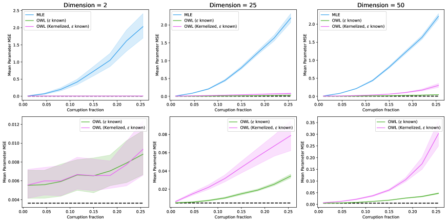
Figure 11: Gaussian results for random corruptions. Dashed black line denotes average performance of MLE on full uncorrupted dataset. Shaded regions denote 95% confidence intervals over 50 random seeds.

Figure 11 presents the random corruption results for estimating a multivariate normal distribution. In contrast with the max-likelihood corruption setting, we see that OWL without kernelization outperforms OWL with kernelization in higher dimensions. It is possible that this is due to the difficulty of density estimation in higher dimensions.

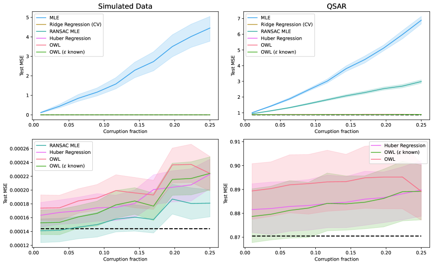
Figure 12: Linear regression results for random corruptions. Dashed black line denotes average performance of MLE on full uncorrupted training set. Shaded regions denote 95% confidence intervals over 50 random seeds.

Figure 12 presents the random corruption results for linear regression. The results here are qualitatively similar to those for the max-likelihood corruption setting, with all three robust methods performing well in the simulated data setting but with RANSAC performing notably worse with QSAR data.

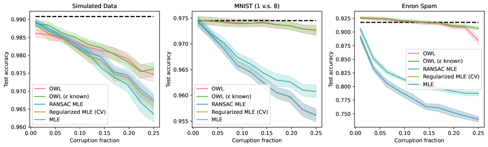
Figure 13: Logistic regression results for random corruptions. Dashed black line denotes average performance of MLE on full uncorrupted training set. Shaded regions denote 95% confidence intervals over 50 random seeds.

Figure 13 presents the random corruption results for logistic regression. As in the max-likelihood corruption case, we see that OWL outperforms the other methods across all three datasets. Moreover, we see that on the Enron spam dataset, OWL even outperforms the uncorrupted MLE baseline, which is entirely possible if the logistic regression model is mis-specified.

Figure 14: Mixture model results for random corruptions. Dashed black line denotes average performance of MLE on full uncorrupted training set. Shaded regions denote 95% confidence intervals over 50 random seeds.

Figure 14 presents the random corruption results for the mixture model settings. The results here are qualitatively similar to those for the max-likelihood corruption setting.

Appendix G More details of the micro-credit study

This section contains additional details of our analysis in Section 7.

Figure 15 shows a scatter-plot for the data and the presence of outliers.

Figure 16 shows the 90% OS-bootstrap confidence bands for the AIT estimates, with the $x$-axis scaled to emphasize the uncertainty for small values of $\epsilon$.

Figure 17 plots minimum-OKL estimate for various values $\epsilon$, along with the associated 90% bootstrap confidence bands.

Figure 18 shows the distribution of profit values for points that were declared as outliers by the OWL procedure at the parameter value $\epsilon_{0}$.

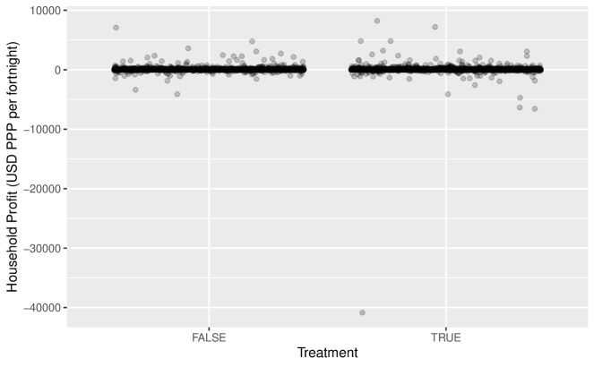
Figure 15: Scatter-plot of the household profit values across treated and non-treated households. Even after removing the household with the extreme profit of -40000 USD PPP, there are still households with extreme profit values that cause brittleness in estimating the average treatment effect.

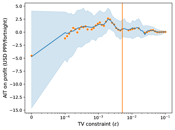
Figure 16: The plot from the left panel of Figure 10, plotted on a re-scaled $x$-axis to emphasize the uncertainty in the AIT estimates for small values of $\epsilon$. The confidence bands become narrow roughly at the tuned value of $\epsilon_{0}=0.005$ (Section 2.2.3), suggesting that the outliers that cause brittleness may have been down-weighted by OWL for $\epsilon=\epsilon_{0}$.

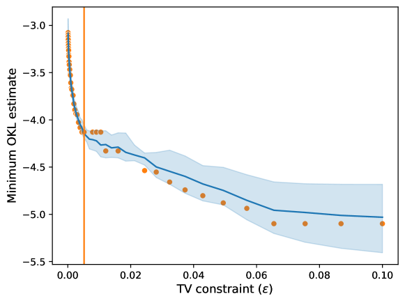
Figure 17: The minimum OKL estimate (i.e. $\hat{R}(\epsilon)=\min_{\theta\in\Theta}\hat{I}_{\epsilon}(\theta)$) versus $\epsilon$ plot for the micro-credit example. Using the notion of curvature in Section 2.2.3, the value $\epsilon_{0}=0.005$ was identified as the point at which this graph has its prominent kink. The $90\%$ confidence bands under $m=50$ OS-bootstrap iterations are also shown.

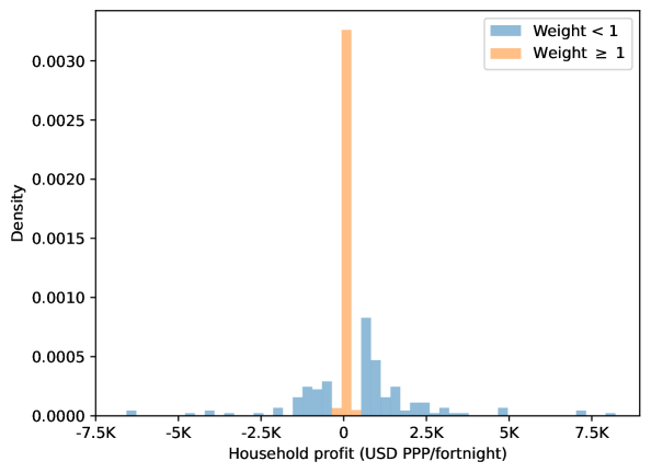
Figure 18: The profit distribution for households that were declared to be inliers ($\{i:w_{i}<1\}$) versus outliers ($\{i:w_{i}\leq 1\}$) by the OWL procedure at parameter $\epsilon_{0}$. For clarity, we omitted an outlying household with a profit value of less that $-40K$ USD PPP.

References

- Agostinelli and Greco [2013] C. Agostinelli and L. Greco. A weighted strategy to handle likelihood uncertainty in Bayesian inference. Computational Statistics, 28(1):319–339, 2013.
- Alquier et al. [2022] P. Alquier, B.-E. Chérief-Abdellatif, A. Derumigny, and J.-D. Fermanian. Estimation of copulas via maximum mean discrepancy. Journal of the American Statistical Association, 0(0):1–16, 2022.
- Amari [2016] S. Amari. Information geometry and its applications. Springer, 2016.
- Andrews and Hemberg [2019] T. S. Andrews and M. Hemberg. M3Drop: Dropout-based feature selection for scRNASeq. Bioinformatics, 35(16):2865–2867, 2019.
- Angelucci et al. [2015] M. Angelucci, D. Karlan, and J. Zinman. Microcredit impacts: Evidence from a randomized microcredit program placement experiment by Compartamos Banco. American Economic Journal: Applied Economics, 7(1):151–182, 2015.
- Barp et al. [2019] A. Barp, F.-X. Briol, A. Duncan, M. Girolami, and L. Mackey. Minimum Stein discrepancy estimators. In Advances in Neural Information Processing Systems, pages 12964–12976, 2019.
- Barratt et al. [2021] S. Barratt, G. Angeris, and S. Boyd. Optimal representative sample weighting. Statistics and Computing, 31(2):1–14, 2021.
- Bartlett and Mendelson [2002] P. L. Bartlett and S. Mendelson. Rademacher and Gaussian complexities: Risk bounds and structural results. Journal of Machine Learning Research, 3:463–482, 2002.
- Basu et al. [1998] A. Basu, I. R. Harris, N. L. Hjort, and M. Jones. Robust and efficient estimation by minimising a density power divergence. Biometrika, 85(3):549–559, 1998.
- Beran [1981] R. Beran. Efficient robust estimates in parametric models. Zeitschrift fuer Wahrscheinlichkeitstheorie und verwwandte Gebiete, 55:91–108, 1981.
- Bernardo and Smith [2009] J. M. Bernardo and A. F. Smith. Bayesian Theory. John Wiley & Sons, 2009.
- Bhatia et al. [2023] K. Bhatia, Y.-A. Ma, A. D. Dragan, P. L. Bartlett, and M. I. Jordan. Bayesian robustness: A nonasymptotic viewpoint. Journal of the American Statistical Association, 0(0):1–25, 2023.
- Billingsley [2013] P. Billingsley. Convergence of probability measures. John Wiley & Sons, 2013.
- Bissiri et al. [2016] P. G. Bissiri, C. C. Holmes, and S. G. Walker. A general framework for updating belief distributions. Journal of the Royal Statistical Society: Series B (Statistical Methodology), 78(5):1103–1130, 2016.
- Boucheron et al. [2005] S. Boucheron, O. Bousquet, and G. Lugosi. Theory of classification: A survey of some recent advances. ESAIM: Probability and Statistics, 9:323–375, 2005.
- Boyd et al. [2011] S. Boyd, N. Parikh, E. Chu, B. Peleato, and J. Eckstein. Distributed optimization and statistical learning via the alternating direction method of multipliers. Foundations and Trends® in Machine learning, 3(1):1–122, 2011.
- Bradic [2016] J. Bradic. Robustness in sparse high-dimensional linear models: Relative efficiency and robust approximate message passing. Electronic Journal of Statistics, 10(2):3894–3944, 2016.
- Bradic et al. [2011] J. Bradic, J. Fan, and W. Wang. Penalized composite quasi-likelihood for ultrahigh dimensional variable selection. Journal of the Royal Statistical Society: Series B (Statistical Methodology), 73(3):325–349, 2011.
- Briol et al. [2019] F.-X. Briol, A. Barp, A. B. Duncan, and M. Girolami. Statistical inference for generative models with maximum mean discrepancy. arXiv preprint arXiv:1906.05944, 2019.
- Broderick et al. [2020] T. Broderick, R. Giordano, and R. Meager. An automatic finite-sample robustness metric: When can dropping a little data make a big difference? arXiv preprint arXiv:2011.14999, 2020.
- Budhiraja and Dupuis [2019] A. Budhiraja and P. Dupuis. Analysis and approximation of rare events. Springer, 2019.
- Chandra et al. [2020] N. K. Chandra, A. Canale, and D. B. Dunson. Escaping the curse of dimensionality in Bayesian model based clustering. arXiv preprint arXiv:2006.02700, 2020.
- Cherief-Abdellatif and Alquier [2020] B.-E. Cherief-Abdellatif and P. Alquier. MMD-Bayes: Robust Bayesian estimation via maximum mean discrepancy. In Proceedings of The 2nd Symposium on Advances in Approximate Bayesian Inference, pages 1–21, 2020.
- Chérief-Abdellatif and Alquier [2022] B.-E. Chérief-Abdellatif and P. Alquier. Finite sample properties of parametric MMD estimation: Robustness to misspecification and dependence. Bernoulli, 28(1):181–213, 2022.
- Claeskens and Hjort [2008] G. Claeskens and N. L. Hjort. Model selection and model averaging. Cambridge University Press, 2008.
- Condat [2016] L. Condat. Fast projection onto the simplex and the ball. Mathematical Programming, 158(1):575–585, 2016.
- Copas [1995] J. Copas. Local likelihood based on kernel censoring. Journal of the Royal Statistical Society: Series B (Methodological), 57(1):221–235, 1995.
- Cover and Thomas [2006] T. M. Cover and J. A. Thomas. Elements of information theory. John Wiley & Sons, second edition, 2006.
- Csiszár [1975] I. Csiszár. I-divergence geometry of probability distributions and minimization problems. The Annals of Probability, 3(1):146–158, 1975.
- Dellaporta et al. [2022] C. Dellaporta, J. Knoblauch, T. Damoulas, and F.-X. Briol. Robust Bayesian inference for simulator-based models via the MMD posterior bootstrap. In Proceedings of The 25th International Conference on Artificial Intelligence and Statistics, pages 943–970, 2022.
- Dembo and Zeitouni [2010] A. Dembo and O. Zeitouni. Large Deviations Techniques and applications. Springer Berlin Heidelberg, 2010.
- Dempster et al. [1977] A. P. Dempster, N. M. Laird, and D. B. Rubin. Maximum likelihood from incomplete data via the EM algorithm. Journal of the Royal Statistical Society: Series B (Methodological), 39(1):1–22, 1977.
- Diakonikolas et al. [2017] I. Diakonikolas, G. Kamath, D. M. Kane, J. Li, A. Moitra, and A. Stewart. Being robust (in high dimensions) can be practical. In Proceedings of the 34th International Conference on Machine Learning, pages 999–1008, 2017.
- Diakonikolas et al. [2019] I. Diakonikolas, D. Kane, S. Karmalkar, E. Price, and A. Stewart. Outlier-robust high-dimensional sparse estimation via iterative filtering. In Advances in Neural Information Processing Systems, 2019.
- Diakonikolas et al. [2020] I. Diakonikolas, S. B. Hopkins, D. Kane, and S. Karmalkar. Robustly learning any clusterable mixture of Gaussians. arXiv preprint arXiv:2005.06417, 2020.
- Dupuis and Morgenthaler [2002] D. J. Dupuis and S. Morgenthaler. Robust weighted likelihood estimators with an application to bivariate extreme value problems. Canadian Journal of Statistics, 30(1):17–36, 2002.
- Eguchi and Copas [1998] S. Eguchi and J. Copas. A class of local likelihood methods and near-parametric asymptotics. Journal of the Royal Statistical Society: Series B (Statistical Methodology), 60(4):709–724, 1998.
- Field and Smith [1994] C. Field and B. Smith. Robust estimation: A weighted maximum likelihood approach. International Statistical Review/Revue Internationale de Statistique, 62(3):405–424, 1994.
- Fong et al. [2021] E. Fong, C. Holmes, and S. G. Walker. Martingale posterior distributions. arXiv preprint arXiv:2103.15671, 2021.
- Gervini and Yohai [2002] D. Gervini and V. J. Yohai. A class of robust and fully efficient regression estimators. The Annals of Statistics, 30(2):583–616, 2002.
- Ghosh and Basu [2016] A. Ghosh and A. Basu. Robust Bayes estimation using the density power divergence. Annals of the Institute of Statistical Mathematics, 68:413–437, 2016.
- Ghourchian et al. [2017] H. Ghourchian, A. Gohari, and A. Amini. Existence and continuity of differential entropy for a class of distributions. IEEE Communications Letters, 21(7):1469–1472, 2017.
- Greco et al. [2008] L. Greco, W. Racugno, and L. Ventura. Robust likelihood functions in Bayesian inference. Journal of Statistical Planning and Inference, 138(5):1258–1270, 2008.
- Green [1984] P. J. Green. Iteratively reweighted least squares for maximum likelihood estimation, and some robust and resistant alternatives. Journal of the Royal Statistical Society: Series B (Methodological), 46(2):149–170, 1984.
- Gretton et al. [2006] A. Gretton, K. Borgwardt, M. Rasch, B. Schölkopf, and A. Smola. A kernel method for the two-sample-problem. In Advances in Neural Information Processing Systems, 2006.
- Grünwald [2011] P. Grünwald. Safe learning: Bridging the gap between Bayes, MDL and statistical learning theory via empirical convexity. In Proceedings of the 24th Annual Conference on Learning Theory, pages 397–420, 2011.
- Hadi and Luceño [1997] A. S. Hadi and A. Luceño. Maximum trimmed likelihood estimators: A unified approach, examples, and algorithms. Computational Statistics & Data Analysis, 25(3):251–272, 1997.
- He et al. [2000] B. He, H. Yang, and S. Wang. Alternating direction method with self-adaptive penalty parameters for monotone variational inequalities. Journal of Optimization Theory and Applications, 106(2):337–356, 2000.
- Hjort and Jones [1996] N. L. Hjort and M. C. Jones. Locally parametric nonparametric density estimation. The Annals of Statistics, 24(4):1619–1647, 1996.
- Hooker and Vidyashankar [2014] G. Hooker and A. N. Vidyashankar. Bayesian model robustness via disparities. TEST, 23(3):556–584, 2014.
- Hu [1997] F. Hu. The asymptotic properties of the maximum-relevance weighted likelihood estimators. Canadian Journal of Statistics, 25(1):45–59, 1997.
- Huber [1964] P. J. Huber. Robust estimation of a location parameter. Ann. Math. Statist., 35(4):73–101, 1964.
- Huber [1981] P. J. Huber. Robust statistics. Wiley, 1981.
- Huber [2011] P. J. Huber. Robust statistics. In International Encyclopedia of Statistical Science, pages 1248–1251. Springer, 2011.
- Huber-Carol et al. [2012] C. Huber-Carol, N. Balakrishnan, M. Nikulin, and M. Mesbah. Goodness-of-fit tests and model validity. Springer Science & Business Media, 2012.
- Hubert and Arabie [1985] L. Hubert and P. Arabie. Comparing partitions. Journal of Classification, 2(1):193–218, 1985.
- Huggins and Miller [2020] J. H. Huggins and J. W. Miller. Robust inference and model criticism using bagged posteriors. arXiv: 1912.07104, 2020.
- Hunsberger [1994] S. Hunsberger. Semiparametric regression in likelihood-based models. Journal of the American Statistical Association, 89(428):1354–1365, 1994.
- Jewson et al. [2018] J. Jewson, J. Q. Smith, and C. Holmes. Principles of Bayesian inference using general divergence criteria. Entropy, 20(6):442, 2018.
- Jiang [2017] H. Jiang. Uniform convergence rates for kernel density estimation. In Proceedings of the 34th International Conference on Machine Learning, pages 1694–1703, 2017.
- Kiseliov [1994] Y. N. Kiseliov. Algorithms of projection of a point onto an ellipsoid. Lithuanian Mathematical Journal, 34(2):141–159, 1994.
- Knoblauch et al. [2018] J. Knoblauch, J. E. Jewson, and T. Damoulas. Doubly robust Bayesian inference for non-stationary streaming data with -divergences. In Advances in Neural Information Processing Systems, pages 64–75, 2018.
- Knoblauch et al. [2022] J. Knoblauch, J. Jewson, and T. Damoulas. An optimization-centric view on Bayes’ rule: Reviewing and generalizing variational inference. Journal of Machine Learning Research, 23(132):1–109, 2022.
- Lawrence et al. [2012] P. W. Lawrence, R. M. Corless, and D. J. Jeffrey. Algorithm 917: Complex double-precision evaluation of the Wright function. ACM Transactions on Mathematical Software (TOMS), 38(3):1–17, 2012.
- Lecué and Lerasle [2020] G. Lecué and M. Lerasle. Robust machine learning by median-of-means: Theory and practice. The Annals of Statistics, 48(2):906–931, 2020.
- LeCun et al. [1998] Y. LeCun, L. Bottou, Y. Bengio, and P. Haffner. Gradient-based learning applied to document recognition. Proceedings of the IEEE, 86(11):2278–2324, 1998.
- Lenth and Green [1987] R. V. Lenth and P. J. Green. Consistency of deviance-based M estimators. Journal of the Royal Statistical Society: Series B (Methodological), 49(3):326–330, 1987.
- Li et al. [2017] H. Li, E. T. Courtois, D. Sengupta, Y. Tan, K. H. Chen, J. J. L. Goh, S. L. Kong, C. Chua, L. K. Hon, W. S. Tan, et al. Reference component analysis of single-cell transcriptomes elucidates cellular heterogeneity in human colorectal tumors. Nature Genetics, 49(5):708–718, 2017.
- Lindsay [1994] B. G. Lindsay. Efficiency versus robustness: The case for minimum Hellinger distance and related methods. The Annals of Statistics, 22(2):1081–1114, 1994.
- Loader [1996] C. R. Loader. Local likelihood density estimation. The Annals of Statistics, 24(4):1602–1618, 1996.
- Lun et al. [2016] A. T. L. Lun, K. Bach, and J. C. Marioni. Pooling across cells to normalize single-cell RNA sequencing data with many zero counts. Genome Biology, 17(1):1–14, 2016.
- Lyddon et al. [2018] S. Lyddon, S. Walker, and C. C. Holmes. Nonparametric learning from Bayesian models with randomized objective functions. In Advances in Neural Information Processing Systems, pages 2075–2085, 2018.
- Lyddon et al. [2019] S. P. Lyddon, C. C. Holmes, and S. G. Walker. General Bayesian updating and the loss-likelihood bootstrap. Biometrika, 106(2):465–478, 2019.
- Majumder et al. [2021] S. Majumder, A. Biswas, T. Roy, S. K. Bhandari, and A. Basu. Statistical inference based on a new weighted likelihood approach. Metrika, 84(1):97–120, 2021.
- Marazzi and Yohai [2004] A. Marazzi and V. J. Yohai. Adaptively truncated maximum likelihood regression with asymmetric errors. Journal of Statistical Planning and Inference, 122(1-2):271–291, 2004.
- Markatou [2000] M. Markatou. Mixture models, robustness, and the weighted likelihood methodology. Biometrics, 56(2):483–486, 2000.
- Markatou et al. [1997] M. Markatou, A. Basu, and B. Lindsay. Weighted likelihood estimating equations: The discrete case with applications to logistic regression. Journal of Statistical Planning and Inference, 57(2):215–232, 1997.
- Markatou et al. [1998] M. Markatou, A. Basu, and B. G. Lindsay. Weighted likelihood equations with bootstrap root search. Journal of the American Statistical Association, 93(442):740–750, 1998.
- Matsubara et al. [2022] T. Matsubara, J. Knoblauch, F.-X. Briol, and C. J. Oates. Robust generalised Bayesian inference for intractable likelihoods. Journal of the Royal Statistical Society: Series B (Statistical Methodology), 84(3):997–1022, 2022.
- Meager [2019] R. Meager. Understanding the average impact of microcredit expansions: A Bayesian hierarchical analysis of seven randomized experiments. American Economic Journal: Applied Economics, 11(1):57–91, 2019.
- Merkle [2014] M. Merkle. Completely monotone functions: A digest. In Analytic Number Theory, Approximation Theory, and Special Functions, pages 347–364. Springer, 2014.
- Metsis et al. [2006] V. Metsis, I. Androutsopoulos, and G. Paliouras. Spam filtering with naive Bayes — which naive Bayes? In CEAS, volume 17, pages 28–69, 2006.
- Miller and Dunson [2019] J. W. Miller and D. B. Dunson. Robust Bayesian Inference via Coarsening. Journal of the American Statistical Association, 114(527):1113–1125, 2019.
- Müller [2013] U. K. Müller. Risk of Bayesian inference in misspecified models, and the sandwich covariance matrix. Econometrica, 81(5):1805–1849, 2013.
- Newton and Raftery [1994] M. A. Newton and A. E. Raftery. Approximate Bayesian inference with the weighted likelihood bootstrap. Journal of the Royal Statistical Society: Series B (Methodological), 56(1):3–26, 1994.
- Olier et al. [2018] I. Olier, N. Sadawi, G. R. Bickerton, J. Vanschoren, C. Grosan, L. Soldatova, and R. D. King. Meta-QSAR: A large-scale application of meta-learning to drug design and discovery. Machine Learning, 107(1):285–311, 2018.
- Parikh and Boyd [2014] N. Parikh and S. Boyd. Proximal algorithms. Foundations and Trends® in Optimization, 1(3):127–239, 2014.
- Pinelis [2020] I. Pinelis. Exact lower and upper bounds on the incomplete gamma function. Mathematical Inequalities and Applications, 23(4):1261, 2020.
- Pompe and Jacob [2021] E. Pompe and P. E. Jacob. Asymptotics of cut distributions and robust modular inference using posterior bootstrap. arXiv preprint arXiv:2110.11149, 2021.
- Pregibon [1982] D. Pregibon. Resistant fits for some commonly used logistic models with medical applications. Biometrics, 38(2):485–498, 1982.
- Rand [1971] W. M. Rand. Objective criteria for the evaluation of clustering methods. Journal of the American Statistical Association, 66(336):846–850, 1971.
- Ressel [1976] P. Ressel. A short proof of Schoenberg’s theorem. Proceedings of the American Mathematical Society, 57(1):66–68, 1976.
- Rigollet and Vert [2009] P. Rigollet and R. Vert. Optimal rates for plug-in estimators of density level sets. Bernoulli, 15(4):1154–1178, 2009.
- Rinaldo and Wasserman [2010] A. Rinaldo and L. Wasserman. Generalized density clustering. The Annals of Statistics, 38(5):2678–2722, 2010.
- Rogers and Hahn [2010] D. Rogers and M. Hahn. Extended-connectivity fingerprints. Journal of Chemical Information and Modeling, 50(5):742–754, 2010.
- Rousseeuw et al. [2011] P. J. Rousseeuw, F. R. Hampel, E. M. Ronchetti, and W. A. Stahel. Robust statistics: The approach based on influence functions. John Wiley & Sons, 2011.
- Samdani et al. [2012] R. Samdani, M.-W. Chang, and D. Roth. Unified expectation maximization. In Proceedings of the 2012 Conference of the North American Chapter of the Association for Computational Linguistics: Human Language Technologies, pages 688–698, 2012.
- Satopaa et al. [2011] V. Satopaa, J. Albrecht, D. Irwin, and B. Raghavan. Finding a “kneedle” in a haystack: Detecting knee points in system behavior. In 31st International Conference on Distributed Computing Systems Workshops, pages 166–171, 2011.
- Shimodaira [2000] H. Shimodaira. Improving predictive inference under covariate shift by weighting the log-likelihood function. Journal of Statistical Planning and Inference, 90(2):227–244, 2000.
- Simon-Gabriel and Schölkopf [2018] C.-J. Simon-Gabriel and B. Schölkopf. Kernel distribution embeddings: Universal kernels, characteristic kernels and kernel metrics on distributions. The Journal of Machine Learning Research, 19(1):1708–1736, 2018.
- Tsou and Royall [1995] T.-S. Tsou and R. M. Royall. Robust likelihoods. Journal of the American Statistical Association, 90(429):316–320, 1995.
- Wang and Zidek [2005] X. Wang and J. V. Zidek. Selecting likelihood weights by cross-validation. The Annals of Statistics, 33(2):463–500, 2005.
- Wang et al. [2004] X. Wang, C. van Eeden, and J. V. Zidek. Asymptotic properties of maximum weighted likelihood estimators. Journal of Statistical Planning and Inference, 119(1):37–54, 2004.
- Windham [1995] M. P. Windham. Robustifying model fitting. Journal of the Royal Statistical Society. Series B (Methodological), 57(3):599–609, 1995.
- Yang and Chen [2018] P. Yang and B. Chen. Robust Kullback-Leibler divergence and universal hypothesis testing for continuous distributions. IEEE Transactions on Information Theory, 65(4):2360–2373, 2018.
- Yatracos [1985] Y. G. Yatracos. Rates of convergence of minimum distance estimators and Kolmogorov’s entropy. The Annals of Statistics, 13(2):768–774, 1985.
- Zellner [1988] A. Zellner. Optimal information processing and Bayes’s theorem. The American Statistician, 42(4):278–280, 1988.
- Zhou et al. [2020] J. Zhou, G. Claeskens, and J. Bradic. Detangling robustness in high dimensions: Composite versus model-averaged estimation. Electronic Journal of Statistics, 14(2):2551–2599, 2020.