Two-fermion lattice Hamiltonian with first and second nearest-neighboring-site interactions

Abstract.

We study the Schrödinger operators ${H}_{\lambda\mu}(K)$, with $K\in\mathbb{T}^{2}$ the fixed quasimomentum of the particles pair, associated with a system of two identical fermions on the two-dimensional lattice $\mathbb{Z}^{2}$ with first and second nearest-neighboring-site interactions of magnitudes $\lambda\in\mathbb{R}$ and $\mu\in\mathbb{R}$, respectively. We establish a partition of the $(\lambda,\mu)-$plane so that in each its connected component, the Schrödinger operator ${H}_{\lambda\mu}(0)$ has a definite (fixed) number of eigenvalues, which are situated below the bottom of the essential spectrum and above its top. Moreover, we establish a sharp lower bound for the number of isolated eigenvalues of ${H}_{\lambda\mu}(K)$ in each connected component.

1. Introduction

Lattice models play an important role in various branches of physics. Among such models are the lattice few-body Hamiltonians [27] that may be viewed as a minimalist version of the corresponding Bose- or Fermi-Hubbard model involving a fixed finite number of particles of a certain type. Surely, the few-body lattice Hamiltonians are of a great theoretic interest already in their own right [2, 4, 5, 16, 17, 19, 21, 23, 24]. In addition, these discrete Hamiltonians may be viewed as a natural approximation for their continuous counterparts [9] allowing to study few-body phenomena in the context of the theory of bounded operators. A still intriguing phenomenon is the celebrated Efimov effect [8] which is proven to take place not only in the continuous case but also in the lattice three-body problems [2, 4, 7, 17]. Furthermore, the discrete Schrödinger operators represent the simplest and natural model for description of few-body systems formed by particles traveling through periodic structures, say, for ulracold atoms injected into optical crystals created by the interference of counter-propagating laser beams [6, 39]. The study of ultracold few-atom systems in optical lattices became very popular in the last years since these systems possess highly controllable parameters such as lattice geometry and dimensionality, particle masses, two-body potentials, temperature etc. (see e.g., [6, 14, 15, 25] and references therein). Unlike the traditional condensed matter systems, where stable composite objects are usually formed by attractive forces, the controllability of the ultracold atomic systems in an optical lattice gives an opportunity to experimentally observe a stable repulsive bound pair of ultracold atoms, see e.g., [33, 39]. Already one-particle one-dimensional lattice Hamiltonians are of interest in applications. For example, in [29], effectively a one-dimensional one-particle lattice Hamiltonian has been employed to exhibit explicitly how an arrangement of molecules of a certain class in lattice structures may enhance the nuclear fusion probability.

Unlike in the continuous case, the lattice few-body system does not admit separation of the center-of-mass motion. However, the discrete translation invariance allows one to use the Floquet-Bloch decomposition (see, e.g., [3, Sec. 4]). In particular, the total $n$-particle lattice Hamiltonian $\mathrm{H}$ in the (quasi)momentum representation may be written as the von Neumann direct integral

$$\mathrm{H}\simeq\int\limits_{K\in\mathbb{T}^{d}}^{\oplus}H(K)\,dK,$$ (1.1)

where $\mathbb{T}^{d}$ is the $d$-dimensional torus and $H(K)$, the fiber Hamiltonian acting in the respective functional Hilbert space on $\mathbb{T}^{(n-1)d}$. Recall that the fiber Hamiltonians $H(K)$ nontrivially depend on the quasimomentum $K\in\mathbb{T}^{d}$ (see e.g., [3, 10, 27, 28]).

It is well known that the Efimov effect [8] that we already mentioned before, was originally attributed to the three-body systems moving in the three-dimensional continuous space $\mathbb{R}^{3}$. The essence of the effect is as follows. A system of three particles in $\mathbb{R}^{3}$ with pairwise attractive short-range potentials has an infinite number of binding energies exponentially converging to zero if the two-particle subsystems do not have a negative spectrum and at least two of them are resonant in the sense that any arbitrarily small negative perturbation of the two-body interaction produces a negative spectrum. A rigorous mathematical proof of the Efimov effect has been given in [34, 36, 38, 40]. In [2, 4, 17], the existence of the Efimov effect has also been proven for three-body systems on the three-dimensional lattice $\mathbb{Z}^{3}$. Later on, the existence of Efimov-type phenomena has been predicted by physicists for a five-boson system moving on a line $\mathbb{R}$ [32], for a four-boson system on the plane $\mathbb{R}^{2}$ [30], and for a system of three spinless fermions moving on the plane $\mathbb{R}^{2}$ [31]. In the latter case, a mathematical proof is available [12, 37], and the phenomenon acquired the name of a super Efimov effect, because of the double exponential convergence of the binding energies to the three-body threshold. One may guess that a similar phenomenon should take place in the system of three spinless fermions on the two-dimensional lattice $\mathbb{Z}^{2}$, at least for some values of the center-of-mass quasimomentum. Surely, in order to prove or disprove this, one needs first to study properties of the system of two spinless fermions on the lattice $\mathbb{Z}^{2}$. In the present work, we are making the first step on this path and study the way how new eigenvalues emerge from the lower and/or upper thresholds of the essential (continuous) spectrum of the fiber Hamiltonians $H(K)$ involved.

In order to obtain a more detail information, we consider an interaction between particles that contains two terms, the one which is only non-trivial if the particles are located in the nearest neighboring sites of the lattice, and another one, only non-trivial if the particles are positioned in the next to nearest neighboring sites (see Sec. 2.1, definition (2.5)). These terms include real factors (coupling constants) $\lambda$ and $\mu$, respectively, and, in the (quasi)momentum representation, the combined interaction potential is denoted by $V_{\lambda\mu}$. The presence in $V_{\lambda\mu}$ of the two terms independent of each other and each depending on the corresponding parameter $\lambda$ and $\mu$ allows the fiber Hamiltonian $H(K)$ to have eigenvalues simultaneously below and above the essential spectrum.

Thus, as the entries $H(K)$ in (1.1), in this work we study the family of the fiber Hamiltonians

$$H_{\lambda\mu}(K):=H_{0}(K)+V_{\lambda\mu},\qquad K=(K_{1},K_{2})\in\mathbb{T}^{2},$$ (1.2)

where $H_{0}(K)$ is the fiber kinetic-energy operator,

$$\bigl{(}H_{0}(K)f\bigr{)}(p)={\mathcal{E}}_{K}(p)f(p),\quad p=(p_{1},p_{2})\in\mathbb{T}^{2},\quad f\in L^{2,o}(\mathbb{T}^{2}),\color[rgb]{0,0,0}$$

with

$${\mathcal{E}}_{K}(p):=2\sum_{i=1}^{2}\Big{(}1-\cos\tfrac{K_{i}}{2}\,\cos p_{i}\Big{)}$$ (1.3)

The potential $V_{\lambda\mu}$ is an integral operator on $L^{2,o}(\mathbb{T}^{2})$ with a smooth kernel function explicitly given by formula (2.9) below. The formula (2.9) implies that for any non-zero $\lambda,\mu$ the operator $V_{\lambda\mu}$ is rank 6. Notice that $V_{\lambda\mu}$ does not depend on $K$ at all. Surely, the operators $H_{0}(K)$ and $V_{\lambda\mu}$, $\lambda,\mu\in\mathbb{R}$, are both bounded and self-adjoint. Since $V_{\lambda\mu}$ is finite rank, the essential spectrum of $H_{\lambda\mu}(K)$ coincides with that of $H_{0}(K)$ (see Sec. 2.4), i.e. it coincides with the segment $[{\mathcal{E}}_{\min}(K),\allowbreak{\mathcal{E}}_{\max}(K)],$ where

$${\mathcal{E}}_{\min}(K):=2\sum\limits_{i=1}^{2}\Big{(}1-\cos\tfrac{K_{i}}{2}\Big{)},\qquad{\mathcal{E}}_{\max}(K):=2\sum\limits_{i=1}^{2}\Big{(}1+\cos\tfrac{K_{i}}{2}\Big{)}.$$

To the best of our knowledge, the Hamiltonian (1.2) represents a new exactly solvable model. Within this model, we will first find both the exact number and location of eigenvalues of the edge operator $H_{\lambda\mu}(0)$. Then, for any pair of the interaction parameters $\lambda,\mu\in\mathbb{R}$, we will establish sharp lower bounds on the numbers of isolated eigenvalues of ${H}_{\lambda\mu}(K),K\neq 0$ lying below and above the essential spectrum Theorem 3.3 and 3.4.

Main goal of the article is to understand the mechanism of emergence of eigenvalues of $H_{\lambda\mu}(K)$ from the essential spectrum as $\lambda$ and $\mu$ vary as well as to clarify the inverse process, the absorption of eigenvalues by the essential spectrum. To achieve this goal, we use as a technical tool, the Fredholm determinants [1, 18]. Namely, we consider the Fredholm determinant $D_{\lambda\mu}(K,z)$ associated with the Lippmann-Schwinger operator generated by the unperturbed Hamiltonian $H_{0}(K)$ and perturbation $V_{\lambda\mu}$. It is well known [1] that for any fixed $K\in\mathbb{T}^{2}$, there is a one-to-one mapping between the set of eigenvalues of the perturbed operator $H_{\lambda\mu}(K)=H_{0}(K)+V_{\lambda\mu}$ and the set of zeros of the associated determinant $D_{\lambda\mu}(K,z)$.

We start with a study of the properties of the the Fredholm determinant $\Delta_{\lambda\mu}(z):=D_{\lambda\mu}(0,z)$ in the edge case $K=0$. Assuming that $C^{-}(\lambda,\mu)$ (resp. $C^{+}(\lambda,\mu)$) is the main (constant) term of the asymptotics of the function $\Delta_{\lambda\mu}(z)$ as $z$ converges to the lower (resp. upper) threshold of the essential spectrum, we show that an additional root of $\Delta_{\lambda\mu}(z)$ emerges below (resp. above) the essential spectrum of $H_{\lambda\mu}(0)$ if and only if $C^{-}(\lambda,\mu)=0$ (resp. $C^{+}(\lambda,\mu)=0$) (see Lemmas 4.4 and 4.8). Therefore, the number of eigenvalues of 1$H_{\lambda\mu}(0)$ changes if and only if the point $(\lambda,\mu)$ on the parameter plane $\mathbb{R}^{2}$ crosses one of the curves $C^{-}(\lambda,\mu)=0$ or $C^{+}(\lambda,\mu)=0$ (see also Lemmas 4.9-4.11). Moreover, after each such a single crossing, the number of eigenvalues of $H_{\lambda\mu}(0)$ changes exactly by one. Surely, this crossing event is interpreted as a moment when the essential spectrum of $H_{\lambda\mu}(0)$ either gives birth to or absorbs a bound state of $H_{\lambda\mu}(0)$(see Theorem 3.4). Furthermore, the curves $C^{-}(\lambda,\mu)=0$ and $C^{+}(\lambda,\mu)=0$ divide the $(\lambda,\mu)$ parameter plane into several simply connected domains on each of which the number of eigenvalues of the operator $H_{\lambda\mu}(0)$ remains constant (see Theorem 3.2).

We notice that in [13, 22] similar results were obtained for a lattice two-boson system. In that case, the description of the partition of the parameter plane $\mathbb{R}^{2}$ into the connected components is quite elementary. In the present, fermionic, case the description of partition of $\mathbb{R}^{2}$ into the connected components is much more complicated and requires a special technique. Surprisingly, the maximum number of isolated eigenvalues is achieved only in four connected components where both $\lambda$ and $\mu$ run through infinite intervals.

The paper is organized as follows. In Sec. 2 we introduce the two-particle Hamiltonian in the position and quasimomentum representations. Sec. 3 contains statements of our main results. In Sec. 4 we present some auxiliary facts that are needed in the proofs of the main results. These proofs themselves are presented in Sec. 5. For convenience of the reader, in Appendix A we give the proof of Lemma 4.7.

2. Hamiltonian of a lattice two-fermion system

2.1. The two-fermion Hamiltonian in the position–space representation

Let $\mathbb{Z}^{2}$ be the two-dimensional lattice and $\ell^{2,a}(\mathbb{Z}^{2}\times\mathbb{Z}^{2})\subset\ell^{2}(\mathbb{Z}^{2}\times\mathbb{Z}^{2})$, the Hilbert space of square–summable antisymmetric functions on $\mathbb{Z}^{2}\times\mathbb{Z}^{2}$.

In the position-space representation, the Hamiltonian $\widehat{\mathbb{H}}_{\lambda\mu}$ associated with a system of two fermions with a first and second nearest-neighboring-site interaction potential $\widehat{\mathbb{V}}_{\lambda\mu}$ is an operator on $\ell^{2,a}(\mathbb{Z}^{2}\times\mathbb{Z}^{2})$ of the following form:

$$\widehat{\mathbb{H}}_{\lambda\mu}=\widehat{\mathbb{H}}_{0}+\widehat{\mathbb{V}}_{\lambda\mu},\,\,\lambda,\mu\in\mathbb{R}.$$ (2.1)

Here, $\widehat{\mathbb{H}}_{0}$ is the kinetic energy operator of the system, defined on $\ell^{2,a}(\mathbb{Z}^{2}\times\mathbb{Z}^{2})$ as

$$[\widehat{\mathbb{H}}_{0}\hat{f}](x_{1},x_{2})=\sum_{s_{1}\in\mathbb{Z}^{2}}\hat{\varepsilon}(x_{1}-s_{1})\hat{f}(s_{1},x_{2})+\sum_{s_{2}\in\mathbb{Z}^{2}}\hat{\varepsilon}(x_{2}-s_{2})\hat{f}(x_{1},s_{2}),\,\,\hat{f}\in\ell^{2,a}(\mathbb{Z}^{2}\times\mathbb{Z}^{2}),$$ (2.2)

where

$${\hat{\varepsilon}(s)=}\left\{\begin{array}[]{ccc}2,\quad\quad|s|=0,\\ -\frac{1}{2},\,\,\quad|s|=1,\\ 0,\quad\quad|s|>1,\end{array}\right.$$ (2.3)

with $|s|=|s_{1}|+|s_{2}|$ for $s=(s_{1},s_{2})\in\mathbb{Z}^{2}$. The first and second nearest-neighboring-site interaction potential $\widehat{\mathbb{V}}_{\lambda\mu}$ is the operator of multiplication by a function $\hat{v}_{\lambda\mu}$,

$$[\widehat{\mathbb{V}}_{\lambda\mu}\hat{f}](x_{1},x_{2})=\hat{v}_{\lambda\mu}(x_{1}-x_{2})\hat{f}(x_{1},x_{2}),\,\,\hat{f}\in\ell^{2,a}(\mathbb{Z}^{2}\times\mathbb{Z}^{2}),$$ (2.4)

where

$$\hat{v}_{\lambda\mu}(s)=\left\{\begin{array}[]{ccc}\frac{\lambda}{2},\quad\quad|s|=1,\\ \frac{\mu}{2},\quad\quad|s|=2,\\ 0,\quad\quad|s|>2.\end{array}\right.$$ (2.5)

Obviously, all the three operators $\widehat{\mathbb{H}}_{0}$, $\widehat{\mathbb{V}}_{\lambda\mu}$, and $\widehat{\mathbb{H}}_{\lambda\mu}$ (for $\lambda,\mu\in\mathbb{R}$) are bounded and self-adjoint.

2.2. The two-fermion Hamiltonian in the quasimomentum representation

Let $\mathbb{T}^{2}$ be the two-dimensional torus, $\mathbb{T}^{2}=(\mathbb{R}/2\pi\mathbb{Z)}^{2}\equiv[-\pi,\pi)^{2}$. The torus $\mathbb{T}^{2}$ represents the Pontryagin dual group of $\mathbb{Z}^{2}$, equipped with the Haar measure $\mathrm{d}p$. Let $L^{2,a}(\mathbb{T}^{2}\times\mathbb{T}^{2})$ be the Hilbert space of square-integrable antisymmetric functions on $\mathbb{T}^{2}\times\mathbb{T}^{2}.$

The quasimomentum-space version of the Hamiltonian (2.1) reads as

$$\mathbb{H}_{\lambda\mu}:=(\mathcal{F}\otimes\mathcal{F})\hat{\mathbb{H}}_{\lambda\mu}(\mathcal{F}\otimes\mathcal{F})^{*},$$

where $\mathcal{F}\otimes\mathcal{F}$ denotes the Fourier transform. The operator $\mathbb{H}_{\lambda\mu}$ acts on $L^{2,a}(\mathbb{T}^{2}\times\mathbb{T}^{2})$ and has the form $\mathbb{H}_{\lambda\mu}=\mathbb{H}_{0}+\mathbb{V}_{\lambda\mu}$, where $\mathbb{H}_{0}=(\mathcal{F}\otimes\mathcal{F})\hat{\mathbb{H}}_{0}(\mathcal{F}\otimes\mathcal{F})^{*}$ is the multiplication operator:

$$[\mathbb{H}_{0}f](p,q)=[\varepsilon(p)+\varepsilon(q)]f(p,q),$$

with

$$\varepsilon(p):=\sum\limits_{i=1}^{2}\big{(}1-\cos p_{i}),\quad p=(p_{1},p_{2})\in\mathbb{T}^{2},$$

the dispersion relation of a single fermion. The interaction $\mathbb{V}_{\lambda\mu}=(\mathcal{F}\otimes\mathcal{F})\hat{\mathbb{V}}_{\lambda\mu}(\mathcal{F}\otimes\mathcal{F})^{*}$ is the integral operator

$$[\mathbb{V}_{\lambda\mu}f](p,q)=\frac{1}{(2\pi)^{2}}\int_{\mathbb{T}^{2}}v_{\lambda\mu}(p-u)f(u,p+q-u)\mathrm{d}u$$

with the kernel function

$$v_{\lambda\mu}(p)=\lambda\sum_{i=1}^{2}\cos p_{i}+\mu\sum_{i=1}^{2}\cos 2p_{i}+2\mu\sum\limits_{i=1}^{2}\sum\limits_{\,i\neq j=1}^{2}\cos p_{i}\cos p_{j},\quad p=(p_{1},p_{2})\in\mathbb{T}^{2}.$$

2.3. The Floquet-Bloch decomposition of $\mathbb{H}_{\lambda\mu}$ and discrete Schrödinger operators

Since $\hat{\mathbb{H}}_{\lambda\mu}$ commutes with the representation of the discrete group $\mathbb{Z}^{2}$ by shift operators on the lattice, the space $L^{2,a}(\mathbb{T}^{2}\times\mathbb{T}^{2})$ and $\mathbb{H}_{\lambda\mu}$ can be decomposed into the von Neumann direct integral as (see, e.g., [3])

$$L^{2,a}(\mathbb{T}^{2}\times\mathbb{T}^{2})\simeq\int_{K\in\mathbb{T}^{2}}^{\oplus}\color[rgb]{0,0,0}L^{2,o}(\mathbb{T}^{2})\,\mathrm{d}K$$ (2.6)

and

$$\mathbb{H}_{\lambda\mu}\simeq\int_{K\in\mathbb{T}^{2}}^{\oplus}\color[rgb]{0,0,0}H_{\lambda\mu}(K)\,\mathrm{d}K,$$ (2.7)

where $L^{2,o}(\mathbb{T}^{2})$ is the Hilbert space of odd functions on $\mathbb{T}^{2}$. The fiber operator $H_{\lambda\mu}(K),$ $K\in\mathbb{T}^{2}$, in (2.7) acting on $L^{2,o}(\mathbb{T}^{2})$ is of the form

$$H_{\lambda\mu}(K):=H_{0}(K)+V_{\lambda\mu},$$ (2.8)

where the (unperturbed) operator $H_{0}(K)$ is the multiplication operator by the function (1.3) and the perturbation operator $V_{\lambda\mu}$ is given by

$$[V_{\lambda\mu}f](s)= \frac{\lambda}{(2\pi)^{2}}\sum\limits_{i=1}^{2}\sin s_{i}\int\limits_{\mathbb{T}^{2}}\sin t_{i}f(t)\mathrm{d}t+\frac{\mu}{(2\pi)^{2}}\sum\limits_{i=1}^{2}\sin 2s_{i}\int\limits_{\mathbb{T}^{2}}\sin 2t_{i}f(t)\mathrm{d}t$$ (2.9)

$$+\frac{\mu}{2\pi^{2}}\sum\limits_{i=1}^{2}\sum\limits_{\,i\neq j=1}^{2}\sin s_{i}\cos s_{j}\int\limits_{\mathbb{T}^{2}}\sin t_{i}\cos t_{j}f(t)\mathrm{d}t.$$

Obviously, both the operators $H_{0}(K)$ and $V_{\lambda\mu}$ are bounded and self-adjoint. In the literature, the parameter $K\in\mathbb{T}^{2}$ is called the two-particle quasimomentum and the entry $H_{\lambda\mu}(K)$ is called the discrete Schrödinger operator associated to the two-particle Hamiltonian $\hat{\mathbb{H}}_{\lambda\mu}.$

2.4. The essential spectrum of discrete Schrödinger operators

Depending on $\lambda,\mu\in\mathbb{R}$, the rank of $V_{\lambda\mu}$ varies but never exceeds six. Hence, by Weyl’s theorem, for any $K\in\mathbb{T}^{2}$ the essential spectrum $\sigma_{\mathrm{ess}}(H_{\lambda\mu}(K))$ of $H_{\lambda\mu}(K)$ coincides with the spectrum of $H_{0}(K),$ i.e.,

$$\sigma_{\mathrm{ess}}(H_{\lambda\mu}(K))=\sigma(H_{0}(K))=[{\mathcal{E}}_{\min}(K),{\mathcal{E}}_{\max}(K)],$$ (2.10)

with

$${\mathcal{E}}_{\min}(K):= \min_{p\in\mathbb{T}^{2}}\,{\mathcal{E}}_{K}(p)=2\sum\limits_{i=1}^{2}\Big{(}1-\cos\tfrac{K_{i}}{2}\Big{)}\geq{\mathcal{E}}_{\min}(0)=0,$$

$${\mathcal{E}}_{\max}(K):= \max_{p\in\mathbb{T}^{2}}\,{\mathcal{E}}_{K}(p)=2\sum\limits_{i=1}^{2}\Big{(}1+\cos\tfrac{K_{i}}{2}\Big{)}\leq{\mathcal{E}}_{\max}(0)=8,$$

where

$${\mathcal{E}}_{K}(p):=2\sum_{i=1}^{2}\Big{(}1-\cos\tfrac{K_{i}}{2}\,\cos p_{i}\Big{)}.$$ (2.11)

3. Main results

Our first main result is the following generalization of Theorems 1 and 2 in [3].

Theorem 3.1.

Suppose that ${H}_{\lambda\mu}(0)$ has $n$ eigenvalues below (resp. above) the essential spectrum for some $\lambda,\mu\in\mathbb{R}.$ Then for each $K\in\mathbb{T}^{2}$ the operator ${H}_{\lambda\mu}(K)$ has at least $n$ eigenvalues below (resp. above) its essential spectrum.

Denote by $\mu^{\pm}_{0}$ and $\mu^{\pm}_{1}$ the following numbers:

$$\mu^{\pm}_{0}=\frac{88-30\pi\pm\sqrt{1044\pi^{2}-6720\pi+10816}}{240\pi-24\pi^{2}-512}\pi,$$ (3.1)

and

$$\mu^{\pm}_{1}=\frac{128-16\pi-9\pi^{2}\pm\sqrt{225\pi^{4}-1440\pi^{3}+3904\pi^{2}-10240\pi+16384}}{120\pi-12\pi^{2}-256}.$$ (3.2)

Note that the numerical values of $\mu^{\pm}_{0}$ and $\mu^{\pm}_{1}$ are as follows:

$$\mu_{0}^{-}=-5.6172...,\quad\mu_{0}^{+}=-2.0623...,\quad\mu_{1}^{-}=-5.7523...,\quad\mu_{1}^{+}=-2.9272...,$$

and, hence, these numbers satisfy the relations

$$\mu^{-}_{1}<\mu_{0}^{-}<\mu^{+}_{1}<\mu^{+}_{0}<0.$$ (3.3)

By using the numbers $\mu_{0}^{+},\mu_{0}^{-}$ and $\mu_{1}^{+},\mu_{1}^{-}$ defined, respectively, in (3.1) and (3.2) we introduce the following two functions on $\mathbb{R}^{2}$:

$$C^{\pm}(\lambda,\mu)=\frac{30\pi-3\pi^{2}-64}{6\pi^{2}}[8(\mu\pm\mu_{0}^{+})(\mu\pm\mu_{0}^{-})\mp\lambda(\mu\pm\mu_{1}^{+})(\mu\pm\mu_{1}^{-})].$$ (3.4)

Obviously, the curves on $(\lambda,\mu)$-plane defined by the equations $C^{\pm}(\lambda,\mu)=0$ coincide with the graphs of the respective functions

$$\lambda(\mu)=\pm\frac{8(\mu\pm\mu_{0}^{+})(\mu\pm\mu_{0}^{-})}{(\mu\pm\mu_{1}^{+})(\mu\pm\mu_{1}^{-})}.\\$$ (3.5)

Any of the two functions (3.5) is differentiable on its domain. The graph of each of them consists of three separate smooth curves with the respective asymptotes $\mu=\mp\mu_{1}^{+}$ and $\mu=\mp\mu_{1}^{-}$. In each case these separate curves divide the plane $\mathbb{R}^{2}$ into the four non-overlapping connected components (see Figs. 1 and 2)

$${\mathcal{C}}_{0}^{-} =\{(\lambda,\mu)\in\mathbb{R}^{2}:\lambda>-\frac{8(\mu-\mu_{0}^{+})(\mu-\mu_{0}^{-})}{(\mu-\mu_{1}^{+})(\mu-\mu_{1}^{-})},\,\,\mu>\mu_{1}^{+}\},$$

$${\mathcal{C}}_{1}^{-} =\{(\lambda,\mu)\in\mathbb{R}^{2}:\,\,\lambda<-\frac{8(\mu-\mu_{0}^{+})(\mu-\mu_{0}^{-})}{(\mu-\mu_{1}^{+})(\mu-\mu_{1}^{-})},\,\,\mu>\mu_{1}^{+}\}$$

$$\quad\quad\cup\{(\lambda,\mu)\in\mathbb{R}^{2}:\,\,\lambda\in\mathbb{R},\,\,\mu=\mu_{1}^{+}\}$$

$$\quad\quad\cup\{(\lambda,\mu)\in\mathbb{R}^{2}:\,\,\lambda>-\frac{8(\mu-\mu_{0}^{+})(\mu-\mu_{0}^{-})}{(\mu-\mu_{1}^{+})(\mu-\mu_{1}^{-})},\,\,\mu_{1}^{-}<\mu<\mu_{1}^{+}\},$$

$${\mathcal{C}}_{2}^{-} =\{(\lambda,\mu)\in\mathbb{R}^{2}:\,\lambda<-\frac{8(\mu-\mu_{0}^{+})(\mu-\mu_{0}^{-})}{(\mu-\mu_{1}^{+})(\mu-\mu_{1}^{-})},\,\,\,\,\mu_{1}^{-}<\mu<\mu_{1}^{+}\}$$

$$\quad\quad\cup\{(\lambda,\mu)\in\mathbb{R}^{2}:\,\,\lambda\in\mathbb{R},\,\,\mu=\mu_{1}^{-}\}$$

$$\quad\quad\cup\{(\lambda,\mu)\in\mathbb{R}^{2}:\,\lambda>-\frac{8(\mu-\mu_{0}^{+})(\mu-\mu_{0}^{-})}{(\mu-\mu_{1}^{+})(\mu-\mu_{1}^{-})},\,\,\,\,\mu<\mu_{1}^{-}\},$$

$${\mathcal{C}}_{3}^{-} =\{(\lambda,\mu)\in\mathbb{R}^{2}:\,\lambda<-\frac{8(\mu-\mu_{0}^{+})(\mu-\mu_{0}^{-})}{(\mu-\mu_{1}^{+})(\mu-\mu_{1}^{-})},\,\,\,\,\mu<\mu_{1}^{-}\}$$

and

$${\mathcal{C}}_{0}^{+} =\{(\lambda,\mu)\in\mathbb{R}^{2}:\lambda<\frac{8(\mu+\mu_{0}^{+})(\mu+\mu_{0}^{-})}{(\mu+\mu_{1}^{+})(\mu+\mu_{1}^{-})},\,\,\mu<-\mu_{1}^{+}\},$$

$${\mathcal{C}}_{1}^{+} =\{(\lambda,\mu)\in\mathbb{R}^{2}:\,\,\lambda>\frac{8(\mu+\mu_{0}^{+})(\mu+\mu_{0}^{-})}{(\mu+\mu_{1}^{+})(\mu+\mu_{1}^{-})},\,\,\mu<-\mu_{1}^{+}\}$$

$$\quad\quad\cup\{(\lambda,\mu)\in\mathbb{R}^{2}:\,\,\lambda\in\mathbb{R},\,\,\mu=-\mu_{1}^{+}\}$$

$$\quad\quad\cup\{(\lambda,\mu)\in\mathbb{R}^{2}:\,\,\lambda<\frac{8(\mu+\mu_{0}^{+})(\mu+\mu_{0}^{-})}{(\mu+\mu_{1}^{+})(\mu+\mu_{1}^{-})},\,\,-\mu_{1}^{+}<\mu<-\mu_{1}^{-}\},$$

$${\mathcal{C}}_{2}^{+} =\{(\lambda,\mu)\in\mathbb{R}^{2}:\,\,\lambda>\frac{8(\mu+\mu_{0}^{+})(\mu+\mu_{0}^{-})}{(\mu+\mu_{1}^{+})(\mu+\mu_{1}^{-})},\,\,-\mu_{1}^{+}<\mu<-\mu_{1}^{-}\}$$

$$\quad\quad\cup\{(\lambda,\mu)\in\mathbb{R}^{2}:\,\,\lambda\in\mathbb{R},\,\,\mu=-\mu_{1}^{-}\}$$

$$\quad\quad\cup\{(\lambda,\mu)\in\mathbb{R}^{2}:\,\lambda<\frac{8(\mu+\mu_{0}^{+})(\mu+\mu_{0}^{-})}{(\mu+\mu_{1}^{+})(\mu+\mu_{1}^{-})},\,\,\,\,\mu>-\mu_{1}^{-}\},$$

$${\mathcal{C}}_{3}^{+} =\{(\lambda,\mu)\in\mathbb{R}^{2}:\,\lambda>\frac{8(\mu+\mu_{0}^{+})(\mu+\mu_{0}^{-})}{(\mu+\mu_{1}^{+})(\mu+\mu_{1}^{-})},\,\,\,\,\mu>-\mu_{1}^{-}\}.$$

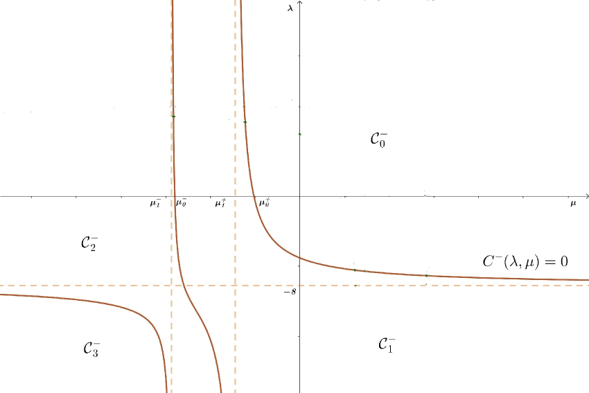
Figure 1. Plot of the curves defined by equation $C^{-}(\lambda,\mu)=0$

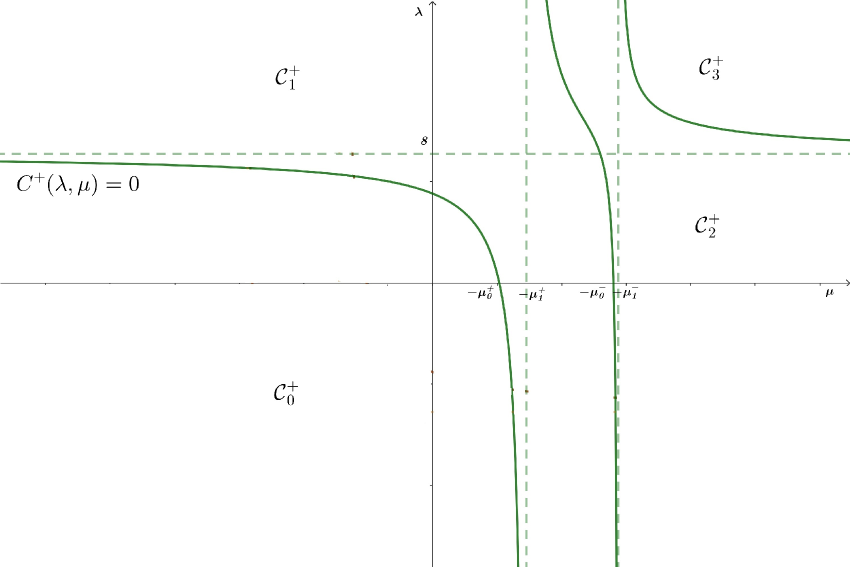
Figure 2. Plot of the curves defined by the equation $C^{+}(\lambda,\mu)=0$

It turns out that in each of the above components ${\mathcal{C}}^{-}_{k}$, the number of eigenvalues of the operator $H_{\lambda\mu}(0)$, lying below its essential spectrum, remains constant. In a similar way, any of the components ${\mathcal{C}}^{+}_{k}$ is a domain where the number of eigenvalues of $H_{\lambda\mu}(0)$, lying above the essential spectrum (2.10), does not vary. Both these facts are established in the following theorem.

Theorem 3.2.

Let ${\mathcal{C}}^{-}$ be one of the above connected components ${\mathcal{C}}^{-}_{k}$, $k=0,1,2,3$, of the partition of the $(\lambda,\mu)$-plane. Then for any $(\lambda,\mu)\in{\mathcal{C}}^{-}$ the number $n_{-}({H}_{\lambda\mu}(0))$ of eigenvalues of $H_{\lambda\mu}(0)$ lying below the essential spectrum $\sigma_{\mathrm{ess}}\bigl{(}H_{\lambda\mu}(0)\bigr{)}$ remains constant. Analogously, let ${\mathcal{C}}^{+}$ be one of the above connected components ${\mathcal{C}}^{+}_{k}$, $k=0,1,2,3$, of the partition of the $(\lambda,\mu)$-plane. Then for any $(\lambda,\mu)\in{\mathcal{C}}^{+}$ the number $n_{+}({H}_{\lambda\mu}(0))$ of eigenvalues of $H_{\lambda\mu}(0)$ lying above $\sigma_{\mathrm{ess}}\bigl{(}H_{\lambda\mu}(0)\bigr{)}$ remains constant.

The result below concerns the number of eigenvalues of the fiber Hamiltonian $H_{\lambda\mu}(K)$ for various $K$ and $(\lambda,\mu)$.

Theorem 3.3.

Let $K\in\mathbb{T}^{2}$ and $(\lambda,\mu)\in\mathbb{R}^{2}$. Then for the numbers $n_{+}({H}_{\lambda\mu}(K))$ and $n_{-}({H}_{\lambda\mu}(K))$ of eigenvalues of the operator $H_{\lambda\mu}(K)$ lying, respectively, above and below its essential spectrum $\sigma_{\mathrm{ess}}\bigl{(}H_{\lambda\mu}(K)\bigr{)}$, the following two series of implications hold:

$$(\lambda,\mu)\in{\mathcal{C}}_{3}^{+}\cap{\mathcal{C}}_{0}^{-} \Longrightarrow\qquad n_{+}({H}_{\lambda\mu}(K))=6,$$ (3.6)

$$(\lambda,\mu)\in{\mathcal{C}}_{2}^{+}\cap{\mathcal{C}}_{0}^{-}\,\mathrm{or}\,(\lambda,\mu)\in{\mathcal{C}}_{2}^{+}\cap{\mathcal{C}}_{1}^{-} \Longrightarrow\qquad n_{+}({H}_{\lambda\mu}(K))\geq 4,$$

$$(\lambda,\mu)\in{\mathcal{C}}_{1}^{+}\cap{\mathcal{C}}_{0}^{-}\,\mathrm{or}\,(\lambda,\mu)\in{\mathcal{C}}_{1}^{+}\cap{\mathcal{C}}_{1}^{-} \Longrightarrow\qquad n_{+}({H}_{\lambda\mu}(K))\geq 2,$$

$$(\lambda,\mu)\in\overline{{\mathcal{C}}_{0}^{+}} \Longrightarrow\qquad n_{+}({H}_{\lambda\mu}(K))\geq 0,$$

and

$$(\lambda,\mu)\in{\mathcal{C}}_{3}^{-}\cap{\mathcal{C}}_{0}^{+} \Longrightarrow\qquad n_{-}({H}_{\lambda\mu}(K))=6,$$ (3.7)

$$(\lambda,\mu)\in{\mathcal{C}}_{2}^{-}\cap{\mathcal{C}}_{0}^{+}\,\mathrm{or}\,(\lambda,\mu)\in{\mathcal{C}}_{2}^{-}\cap{\mathcal{C}}_{1}^{+} \Longrightarrow\qquad n_{-}({H}_{\lambda\mu}(K))\geq 4,$$

$$(\lambda,\mu)\in{\mathcal{C}}_{1}^{-}\cap{\mathcal{C}}_{0}^{+}\,\mathrm{or}\,(\lambda,\mu)\in{\mathcal{C}}_{1}^{-}\cap{\mathcal{C}}_{1}^{+} \Longrightarrow\qquad n_{-}({H}_{\lambda\mu}(K))\geq 2,$$

$$(\lambda,\mu)\in\overline{{\mathcal{C}}_{0}^{-}} \Longrightarrow\qquad n_{-}({H}_{\lambda\mu}(K))\geq 0,$$

where $\overline{\mathcal{A}}$ is the closure of the set $\mathcal{A}$.

The next theorem establishes the exact number of eigenvalues of $H_{\lambda\mu}(0)$ outside its essential spectrum. In particular, it shows that the estimates for the numbers $n_{+}({H}_{\lambda\mu}(K))$ and $n_{-}({H}_{\lambda\mu}(K))$ of eigenvalues of the operator ${H}_{\lambda\mu}(K)$ obtained in Theorem 3.3 are sharp.

Theorem 3.4.

For various $\lambda,\mu\in\mathbb{R}$, the numbers and multiplicities of eigenvalues of $H_{\lambda\mu}(0)$ outside the set $\sigma_{\mathrm{ess}}\bigl{(}H_{\lambda\mu}(0)\bigr{)}$ are described in the following statements.

• For any $(\lambda,\mu)\in{\mathcal{C}}_{30}={\mathcal{C}}_{3}^{-}$ the operator $H_{\lambda\mu}(0)$ has exactly three eigenvalues $z_{1}(\lambda,\mu;0)$, $z_{2}(\lambda,\mu;0)$ and $z_{3}(\lambda,\mu;0)$ of multiplicity two satisfying

  $$z_{1}(\lambda,\mu;0)<z_{2}(\lambda,\mu;0)<z_{3}(\lambda,\mu;0)<0.$$ (3.8)

• For any $(\lambda,\mu)\in{\mathcal{C}}_{20}:={\mathcal{C}}_{2}^{-}\cap{\mathcal{C}}_{0}^{+}$ the operator $H_{\lambda\mu}(0)$ has two eigenvalues $z_{1}(\lambda,\mu;0)$ and $z_{2}(\lambda,\mu;0)$ of multiplicity two satisfying

  $$z_{1}(\lambda,\mu;0)<z_{2}(\lambda,\mu;0)<0$$ (3.9)

  and it has no eigenvalues in $(8,+\infty)$

• For any $(\lambda,\mu)\in{\mathcal{C}}_{21}:={\mathcal{C}}_{2}^{-}\cap{\mathcal{C}}_{1}^{+}$, the operator $H_{\lambda\mu}(0)$ has two eigenvalues $z_{1}(\lambda,\mu;0)$ and $z_{2}(\lambda,\mu;0)$ of multiplicity two in $(-\infty,0)$ and it has one eigenvalue of multiplicity two in $(8,+\infty)$.

• For any $(\lambda,\mu)\in{\mathcal{C}}_{11}:={\mathcal{C}}_{1}^{-}\cap{\mathcal{C}}_{1}^{+}$, the operator $H_{\lambda\mu}(0)$ has two eigenvalues $z_{1}(\lambda,\mu)<0$ and $z_{2}(\lambda,\mu)>8$ of multiplicity two .

• For any $(\lambda,\mu)\in{\mathcal{C}}_{10}:={\mathcal{C}}_{1}^{-}\cap{\mathcal{C}}_{0}^{+}$, the operator $H_{\lambda\mu}(0)$ has one eigenvalue $z(\lambda,\mu;0)$ of multiplicity two in $(-\infty,0)$, nevertheless it has no eigenvalues in $(8,+\infty)$.

• For any $(\lambda,\mu)\in{\mathcal{C}}_{00}:={\mathcal{C}}_{0}^{-}\cap{\mathcal{C}}_{0}^{+}$, the operator $H_{\lambda\mu}(0)$ has no eigenvalues outside of the essential spectrum.

• For any $(\lambda,\mu)\in{\mathcal{C}}_{01}:={\mathcal{C}}_{0}^{-}\cap{\mathcal{C}}_{1}^{+}$, the operator $H_{\lambda\mu}(0)$ has one eigenvalue $z(\lambda,\mu;0)$ of multiplicity two in $(8,+\infty)$ and it has no eigenvalues in $(-\infty,0)$.

• For any $(\lambda,\mu)\in{\mathcal{C}}_{02}:={\mathcal{C}}_{0}^{-}\cap{\mathcal{C}}_{2}^{+}$, the operator $H_{\lambda\mu}(0)$ has two eigenvalues $z_{1}(\lambda,\mu;0)$ and $z_{2}(\lambda,\mu;0)$ of multiplicity two satisfying

  $$8<z_{2}(\lambda,\mu;0)<z_{1}(\lambda,\mu;0)$$ (3.10)

  and it has no eigenvalues in $(-\infty,0)$.

• For any $(\lambda,\mu)\in{\mathcal{C}}_{12}={\mathcal{C}}_{1}^{-}\cap{\mathcal{C}}_{2}^{+}$, the operator $H_{\lambda\mu}(0)$ has one eigenvalue of multiplicity two in $(-\infty,0)$ and it has two eigenvalues $z_{1}(\lambda,\mu;0)$ and $z_{2}(\lambda,\mu;0)$ of multiplicity two in $(8,+\infty)$.

• For any $(\lambda,\mu)\in{\mathcal{C}}_{03}:={\mathcal{C}}_{3}^{+}$, the operator $H_{\lambda\mu}(0)$ has exactly three eigenvalues $z_{1}(\lambda,\mu;0)$, $z_{2}(\lambda,\mu;0)$ and $z_{3}(\lambda,\mu;0)$ of multiplicity two satisfying

  $$8<z_{3}(\lambda,\mu;0)<z_{2}(\lambda,\mu;0)<z_{1}(\lambda,\mu;0).$$ (3.11)

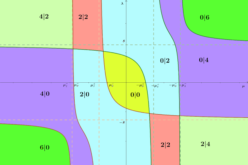
Figure 3. Partition of the $(\lambda,\mu)$-plane of parameters $\lambda,\mu\in\mathbb{R}$ in the connected components ${\mathcal{C}}_{\alpha\beta},\alpha,\beta=0,1,2,3$ (see Theorem 3.4). These components are tagged by the symbols $N_{-}|N_{+}$ formed of the numbers $N_{-}:=n_{-}(H_{\lambda,\mu}(0))$ and $N_{+}:=n_{+}(H_{\lambda,\mu}(0))$ of eigenvalues of $H_{\lambda\mu}(0)$ lying below and above the essential spectrum, respectively. Until the point $(\lambda,\mu)$ does not cross any of the borders between ${\mathcal{C}}_{\alpha\beta}$, no change occurs in $N_{-}$ and $N_{+}$. However, as soon as $(\lambda,\mu)$ crosses one of those borders, the essential spectrum of $H_{\lambda\mu}(0)$ either gives birth or absorbs eigenvalues of $H_{\lambda\mu}(0)$.

4. Auxiliary statements

Let $L^{2,\mathrm{os}}(\mathbb{T}^{2})\subset L^{2,\mathrm{o}}(\mathbb{T}^{2})$ and $L^{2,\mathrm{oa}}(\mathbb{T}^{2})\subset L^{2,\mathrm{o}}(\mathbb{T}^{2})$ be the subspaces of odd-symmetric and odd-antisymmetric functions defined as

$$L^{2,\mathrm{os}}(\mathbb{T}^{2})=\{{f}\in L^{2,o}(\mathbb{T}^{2}):{f}(p_{1},p_{2})={f}(p_{2},p_{1}),\mbox{for a.e}\,\,(p_{1},p_{2})\in\mathbb{T}^{2}\}$$

and

$$L^{2,\mathrm{oa}}(\mathbb{T}^{2})=\{{f}\in L^{2,o}(\mathbb{T}^{2}):{f}(p_{1},p_{2})=-{f}(p_{2},p_{1}),\mbox{for a.e}\,\,(p_{1},p_{2})\in\mathbb{T}^{2}\},$$

respectively.

Lemma 4.1.

The equality

$$L^{2,\mathrm{o}}(\mathbb{T}^{2})=L^{2,\mathrm{os}}(\mathbb{T}^{2})\oplus L^{2,\mathrm{oa}}(\mathbb{T}^{2})$$ (4.1)

holds true.

Proof.

The proof follows from the fact that each element of $L^{2,\mathrm{o}}(\mathbb{T}^{2})$ may be represented as the sum of a function in $L^{2,\mathrm{os}}(\mathbb{T}^{2})$ and a function in $L^{2,\mathrm{oa}}(\mathbb{T}^{2})$.∎

The operator $H_{0}(0)$ is the multiplication operator by the symmetric function ${\mathcal{E}}_{0}(p)=2\varepsilon(p)=2\varepsilon(p_{1},p_{2})$ in $L^{2,o}(\mathbb{T}^{2}).$ Hence, for each $\theta\in\{\mathrm{os},\mathrm{oa}\}$ the subspace $L^{2,\theta}(\mathbb{T}^{2})$ is invariant with respect to $H_{0}(0).$ Now recall that the interaction operator $V_{\lambda\mu}$ has the form (2.9) and, thus, it reads as

$$[V_{\lambda\mu}f](p)= \frac{\lambda}{(2\pi)^{2}}\int\limits_{\mathbb{T}^{2}}(\sin p_{1}\sin q_{1}+\sin p_{2}\sin q_{2})f(q)\mathrm{d}q$$

$$+\frac{\mu}{(2\pi)^{2}}\int\limits_{\mathbb{T}^{2}}(\sin 2p_{1}\sin 2q_{1}+\sin 2p_{2}\sin 2q_{2})f(q)\mathrm{d}q$$

$$+\frac{\mu}{2\pi^{2}}\int\limits_{\mathbb{T}^{2}}(\sin p_{1}\cos p_{2}\sin q_{1}\cos q_{2}+\sin p_{2}\cos p_{1}\sin q_{2}\cos q_{1})f(q)\mathrm{d}q.$$

By applying the equalities

$$2\sin p_{1}\sin q_{1} +2\sin p_{2}\sin q_{2}$$

$$=(\sin p_{1}+\sin p_{2})(\sin q_{1}+\sin q_{2})+(\sin p_{1}-\sin p_{2})(\sin q_{1}-\sin q_{2}),$$

$$2\sin 2p_{1}\sin 2 q_{1}+2\sin 2p_{2}\sin 2q_{2}$$

$$=(\sin 2p_{1}+\sin 2p_{2})(\sin 2q_{1}+\sin 2q_{2})+(\sin 2p_{1}-\sin 2p_{2})(\sin 2q_{1}-\sin 2q_{2}),$$

$$2\sin p_{1}\cos p_{2} \sin q_{1}\cos q_{2}+2\sin p_{2}\cos p_{1}\sin q_{2}\cos q_{1}$$

$$=(\sin p_{1}\cos p_{2}+\sin p_{2}\cos p_{1})(\sin q_{1}\cos q_{2}+\sin q_{2}\cos q_{1})$$

$$+(\sin p_{1}\cos p_{2}-\sin p_{2}\cos p_{1})(\sin q_{1}\cos q_{2}-\sin q_{2}\cos q_{1})$$

and denoting by ${V}_{\lambda\mu}^{\mathrm{\theta}}$ the respective part of ${V}_{\lambda\mu}$ in the reducing subspace $L^{2,\theta}(\mathbb{T}^{2}),\,\theta\in\{\mathrm{os},\mathrm{oa}\}$, we arrive at the expressions

$$[{V}_{\lambda\mu}^{\mathrm{os}}{f}](p)= \frac{\lambda}{8\pi^{2}}(\sin p_{1}+\sin p_{2})\int\limits_{\mathbb{T}^{2}}(\sin q_{1}+\sin q_{2})f(q)\mathrm{d}q$$

$$+\frac{\mu}{8\pi^{2}}(\sin 2p_{1}+\sin 2p_{2})\int\limits_{\mathbb{T}^{2}}(\sin 2q_{1}+\sin 2q_{2})f(q)\mathrm{d}q$$

$$+\frac{\mu}{4\pi^{2}}(\sin p_{1}\cos p_{2}+\sin p_{2}\cos p_{1})\int\limits_{\mathbb{T}^{2}}(\sin q_{1}\cos q_{2}+\sin q_{2}\cos q_{1})f(q)\mathrm{d}q$$

and

$$[{V}_{\lambda\mu}^{\mathrm{oa}}{f}](p)= \frac{\lambda}{8\pi^{2}}(\sin p_{1}-\sin p_{2})\int\limits_{\mathbb{T}^{2}}(\sin q_{1}-\sin q_{2})f(q)\mathrm{d}q$$

$$+\frac{\mu}{8\pi^{2}}(\sin 2p_{1}-\sin 2p_{2})\int\limits_{\mathbb{T}^{2}}(\sin 2q_{1}-\sin 2q_{2})f(q)\mathrm{d}q$$

$$+\frac{\mu}{4\pi^{2}}(\sin p_{1}\cos p_{2}-\sin p_{2}\cos p_{1})\int\limits_{\mathbb{T}^{2}}(\sin q_{1}\cos q_{2}-\sin q_{2}\cos q_{1})f(q)\mathrm{d}q.$$

It follows from the above expressions that

$${H}_{\lambda\mu}(0)\big{|}_{L^{2,\theta}(\mathbb{T}^{2})}={H}_{\lambda\mu}^{\theta}(0):=H_{0}+{V}_{\lambda\mu}^{\theta},\,\,\text{for}\,\,\theta\in\{\mathrm{os},\mathrm{oa}\}.$$

Therefore,

$$\sigma\Big{(}{H}_{\lambda\mu}(0)\Big{)}=\bigcup_{\theta\in\{\mathrm{os},\mathrm{oa}\}}\sigma\Big{(}{H}_{\lambda\mu}(0)\big{|}_{L^{2,\theta}(\mathbb{T}^{2})}\Big{)},$$ (4.2)

where $A\big{|}_{\mathcal{H}}$ is the restriction of a self-adjoint operator $A$ on a reducing subspace ${\mathcal{H}}$. Thus, the study of the discrete spectrum of ${H}_{\lambda\mu}(0)$ reduces to that for the restrictions of ${H}_{\lambda\mu}(0)$ onto each subspace $L^{2,\theta}(\mathbb{T}^{2})$, $\theta\in\{\mathrm{os},\mathrm{oa}\}$.

4.1. The Lippmann–Schwinger operator

Let $\{\alpha_{i}^{\theta},\,\,i=1,2,3\}$ be a system of vectors in $L^{2,\theta}(\mathbb{T}^{2}),\,\theta\in\{\mathrm{os},\mathrm{oa}\}$, with

$$\alpha_{1}^{os}(p)=\dfrac{\sin p_{1}+\sin p_{2}}{2\pi},\,\,\alpha_{2}^{os}(p)=\dfrac{\sin 2p_{1}+\sin 2p_{2}}{2\pi},\,\,\alpha_{3}^{os}(p)=\dfrac{\sin p_{1}\cos p_{2}+\sin p_{2}\cos p_{1}}{\sqrt{2}\pi}$$ (4.3)

and

$$\alpha_{1}^{oa}(p)=\dfrac{\sin p_{1}-\sin p_{2}}{2\pi},\,\,\alpha_{2}^{oa}(p)=\dfrac{\sin 2p_{1}-\sin 2p_{2}}{2\pi},\,\,\alpha_{3}^{oa}(p)=\dfrac{\sin p_{1}\cos p_{2}-\sin p_{2}\cos p_{1}}{\sqrt{2}\pi}.$$ (4.4)

One easily verifies by inspection that the vectors (4.3) and (4.4) are orthonormal in $L^{2,o}(\mathbb{T}^{2})$. By using the orthonormal systems (4.3) and (4.4) one obtains

$${V}_{\lambda\mu}^{\theta}{f}=\frac{\lambda}{2}({f},\alpha_{1}^{\theta})\alpha_{1}^{\theta}+\frac{\mu}{2}({f},\alpha_{2}^{\theta})\alpha_{2}^{\theta}+\frac{\mu}{2}({f},\alpha_{3}^{\theta})\alpha_{3}^{\theta},\quad\theta\in\{\mathrm{os},\,\,\mathrm{oa}\},$$ (4.5)

where $(\cdot,\cdot)$ is the inner product in $L^{2,\theta}(\mathbb{T}^{2}).$ For any $z\in\mathbb{C}\setminus[0,\,8]$ we define (the transpose of) the Lippmann-Schwinger operator (see., e.g., [26]) as

$${B}_{\lambda\mu}^{\theta}(0,z)=-{V}_{\lambda\mu}^{\theta}{R}_{0}(0,z),\,\theta\in\{\mathrm{os},\mathrm{oa}\},$$

where ${R}_{0}(0,z):=[{H}_{0}(0)-zI]^{-1},\,z\in\mathbb{C}\setminus[0,\,8]$, is the resolvent of the operator ${H}_{0}(0)$.

Lemma 4.2.

For each $\lambda,\mu\in\mathbb{R}$ the number $z\in\mathbb{C}\setminus[0,\,8]$ is an eigenvalue of the operator ${H}_{\lambda\mu}^{\theta}(0)$ if and only if the number $1$ is an eigenvalue for ${B}_{\lambda\mu}^{\theta}(0,z),\,\theta\in\{\mathrm{os},\mathrm{oa}\}$.

The proof of this lemma is quite standard (see., e.g., [1]) and, thus, we omit it.

In the following, we identify the symbols $os$ and $oa$ with the signs $\mathrm{+}$ and $\mathrm{-}$, respectively.

The representation (4.5) yields the equivalence of the Lippmann-Schwinger equation

$${B}_{\lambda\mu}^{\theta}(0,z){\varphi}={\varphi},\,\,\,{\varphi}\in L^{2,\theta}(\mathbb{T}^{2}),\,\theta\in\{\mathrm{os},\mathrm{oa}\}$$

to the following algebraic linear system in $x_{i}:=({\varphi},\alpha_{i}^{\theta}),\,\,i=1,2,3$:

$$\left\{\begin{array}[]{ccc}(1+\lambda a^{\pm}(z))x_{1}+\lambda c^{\pm}(z)x_{2}+\lambda d^{\pm}(z)x_{3}=0,\\ \mu c^{\pm}(z)x_{1}+(1+\mu b^{\pm}(z))x_{2}+\mu e^{\pm}(z)x_{3}=0,\\ 2\mu d^{\pm}(z)x_{1}+2\mu e^{\pm}(z)x_{2}+(1+\mu f^{\pm}(z))x_{3}=0,\\ \end{array}\right.$$ (4.6)

where

$$a^{\pm}(z)=\frac{1}{8\pi^{2}}\int\limits_{\mathbb{T}^{2}}\frac{(\sin p_{1}\pm\sin p_{2})^{2}\ \mathrm{d}p}{{\mathcal{E}}_{0}(p)-z},$$ (4.7)

$$b^{\pm}(z)=\frac{1}{8\pi^{2}}\int\limits_{\mathbb{T}^{2}}\frac{(\sin 2p_{1}\pm\sin 2p_{2})^{2}\ \mathrm{d}p}{{\mathcal{E}}_{0}(p)-z},$$ (4.8)

$$c^{\pm}(z)=\frac{1}{8\pi^{2}}\int\limits_{\mathbb{T}^{2}}\frac{(\sin p_{1}\pm\sin p_{2})(\sin 2p_{1}\pm\sin 2p_{2})\mathrm{d}p}{{\mathcal{E}}_{0}(p)-z},$$ (4.9)

$$d^{\pm}(z)=\frac{\sqrt{2}}{8\pi^{2}}\int\limits_{\mathbb{T}^{2}}\frac{(\sin p_{1}\pm\sin p_{2})(\sin p_{1}\cos p_{2}\pm\sin p_{2}\cos p_{1})\mathrm{d}p}{{\mathcal{E}}_{0}(p)-z},$$ (4.10)

$$e^{\pm}(z)=\frac{\sqrt{2}}{8\pi^{2}}\int\limits_{\mathbb{T}^{2}}\frac{(\sin 2p_{1}\pm\sin 2p_{2})(\sin p_{1}\cos p_{2}\pm\sin p_{2}\cos p_{1})\mathrm{d}p}{{\mathcal{E}}_{0}(p)-z},$$ (4.11)

$$f^{\pm}(z)=\frac{1}{2\pi^{2}}\int\limits_{\mathbb{T}^{2}}\frac{(\sin p_{1}\cos p_{2}\pm\sin p_{2}\cos p_{1})^{2}\mathrm{d}p}{{\mathcal{E}}_{0}(p)-z}.$$ (4.12)

It is easy to check that the functions $a^{\pm}(z),b^{\pm}(z),c^{\pm}(z),d^{\pm}(z),e^{\pm}(z)$ and $f^{\pm}(z)$ do not depend on the sign $\pm$. Thus, we skip the sign superscripts and denote these functions simply by $a(z),b(z),c(z),d(z),e(z)$ and $f(z)$.

Remark 4.3.

One easily verifies by inspection that the following relations hold:

$$b(z)+\sqrt{2}e(z)=(4-z)\,c(z),$$

$$\sqrt{2}e(z)+f(z)=\sqrt{2}\,(4-z)\,d(z),$$

$$c(z)+\sqrt{2}\,d(z)=(4-z)\,a(z)+\frac{1}{2}.$$

The reasoning similar to the one we used in the case of the functions (4.7)–(4.12) allows us to conclude that the determinant of the operator $I-{B}_{\lambda\mu}^{\theta}(0,z)$ does not depend on $\theta$, too. Thus we write

$$\Delta_{\lambda\mu}(z):=\Delta_{\lambda\mu}^{\theta}(z):=\mathop{\mathrm{det}}[I-{B}_{\lambda\mu}^{\theta}(0,z)],\,\,z\in\mathbb{C}\setminus[0,\,8],\,\theta\in\{\mathrm{os},\mathrm{oa}\}.$$

Lemma 4.4.

A number $z\in\mathbb{C}\setminus[0,\,8]$ is an eigenvalue of the operator ${H}_{\lambda\mu}(0)$ if and only if

$$\Delta_{\lambda\mu}(z)=0.$$ (4.13)

If $z$ is such an eigenvalue then necessarily it has multiplicity two.

The proof of this lemma for each $\theta\in\{\mathrm{os},\mathrm{oa}\}$ is quite standard (cf., e.g., [22, 20])

Remark 4.5.

Notice that for each $\theta\in\{\mathrm{os},\mathrm{oa}\}$ any eigenvalue $z\in\mathbb{C}\setminus[0,\,8]$ of ${H}^{\theta}_{\lambda\mu}(0)$ is simple. Since ${H}_{\lambda\mu}(0)={H}^{os}_{\lambda\mu}(0)\oplus{H}^{oa}_{\lambda\mu}(0)$, the same $z$ is an eigenvalue of multiplicity two for ${H}_{\lambda\mu}(0)$.

Lemma 4.6.

For any $\lambda,\mu\in\mathbb{R}$ the determinant $\Delta_{\lambda\mu}(z)$ has the form

$$\Delta_{\lambda\mu}(z)=\Delta_{\lambda 0}(z)\Delta_{0\mu}(z)+\Delta^{(12)}_{\lambda\mu}(z),$$ (4.14)

where

$$\Delta_{\lambda 0}(z)=1+\lambda a(z),$$ (4.15)

$$\Delta_{0\mu}(z)=(1+\mu b(z))(1+\mu f(z))-2\mu^{2}e^{2}(z),\color[rgb]{0,0,0}$$ (4.16)

$$\Delta^{(12)}_{\lambda\mu}(z)=4\lambda\mu^{2}c(z)d(z)e(z)-\lambda\mu c^{2}(z)(1+\mu f(z))-2\lambda\mu d^{2}(z)(1+\mu b(z)).$$ (4.17)

Proof.

Direct computation of the determinant gives the result. ∎

Lemma 4.7.

The functions $a(z),b(z),c(z),d(z),e(z)$ and $f(z)$ defined in $\mathbb{R}\setminus[0,8]$ are real-valued and, moreover, strictly increasing and positive in $(-\infty,0)$, strictly increasing and negative in $(8,+\infty)$ and have following asymptotics:

$$\lim\limits_{z\nearrow 0}a(z)=\frac{\pi-2}{2\pi},\quad\lim\limits_{z\nearrow 0}b(z)=\frac{30\pi-92}{3\pi},\quad\lim\limits_{z\nearrow 0}c(z)=\frac{2\pi-6}{\pi},$$ (4.18)

$$\lim\limits_{z\nearrow 0}d(z)=\frac{4-\pi}{2\sqrt{2}\pi},\quad\lim\limits_{z\nearrow 0}e(z)=\frac{20-6\pi}{3\sqrt{2}\pi},\quad\lim\limits_{z\nearrow 0}f(z)=\frac{4}{3\pi}$$ (4.19)

and

$$\lim\limits_{z\searrow 8}a(z)=\frac{2-\pi}{2\pi},\quad\lim\limits_{z\searrow 8}b(z)=\frac{92-30\pi}{3\pi},\quad\lim\limits_{z\searrow 8}c(z)=\frac{6-2\pi}{\pi},$$ (4.20)

$$\lim\limits_{z\searrow 8}d(z)=\frac{\pi-4}{2\sqrt{2}\pi},\quad\lim\limits_{z\searrow 8}e(z)=\frac{6\pi-20}{3\sqrt{2}\pi},\quad\lim\limits_{z\searrow 8}f(z)=-\frac{4}{3\pi}.$$ (4.21)

The proof of Lemma 4.7 is given in Appendix A. $\square$

Lemma 4.8.

The function $\Delta_{\lambda\mu}(z)$ is real-valued on $\mathbb{R}\setminus[0,8]$ and has the following asymptotics:

$$\Delta_{\lambda\mu}(z)=C^{-}(\lambda,\mu)+o(1),\,\,\text{as}\,\,z\nearrow 0,$$ (4.22)

$$\Delta_{\lambda\mu}(z)=C^{+}(\lambda,\mu)+o(1),\,\,\text{as}\,\,z\searrow 8,$$ (4.23)

where the functions $C^{\pm}(\lambda,\mu)$ are given by (3.4).

Proof.

In view of Lemmas 4.6 and 4.7, the proof is obtained by an immediate inspection taking into account the definitions (3.1) and (3.2). ∎

Next we study the number and location of roots of the functions $\Delta_{\lambda 0}$ and $\Delta_{0\mu}$ defined by (4.15) and (4.16).

Lemma 4.9.

Let $\lambda\in\mathbb{R}.$

• If $\lambda<\frac{2\pi}{2-\pi},$ then $\Delta_{\lambda 0}(\cdot)$ has a unique root $\zeta^{-}(\lambda,0)$ in $(-\infty,0)$, and it has no roots in $(8,+\infty)$.

• If $\lambda\in[\frac{2\pi}{2-\pi},\frac{2\pi}{\pi-2}],$ then $\Delta_{\lambda 0}(\cdot)$ has no roots in $\mathbb{R}\setminus[0,8]$.

• If $\lambda>\frac{2\pi}{\pi-2},$ then $\Delta_{\lambda 0}(\cdot)$ has a unique root $\zeta^{+}(\lambda,0)$ in $(8,+\infty)$, and it has no roots in $(-\infty,0)$.

Lemma 4.10.

Let $\mu\in\mathbb{R}$ and let $\mu_{0}^{-}$ be as in (3.1). Then:

• For any $\mu<\mu_{0}^{-}$ the functions $1+\mu b(z)$ and $1+\mu f(z)$ have unique roots $\eta^{(-)}_{1}(\mu)$ and $\eta^{(-)}_{2}(\mu)$ in $(-\infty,0),$ respectively.

• For any $\mu>-\mu_{0}^{-}$ the functions $1+\mu b(z)$ and $1+\mu f(z)$ have unique roots $\eta^{(+)}_{1}(\mu)$ and $\eta^{(+)}_{2}(\mu)$ in $(8,+\infty),$ respectively.

Proof.

Both Lemmas 4.9 and 4.10 are proven by using the representations (4.15) and (4.16) from Lemma 4.6 and the asymptotical formulae for $a(z)$, $b(z)$ and $f(z)$ from Lemma 4.7.∎

Let $\eta^{(-)}_{1}(\mu)$, $\eta^{(-)}_{2}(\mu)$ and $\eta^{(+)}_{1}(\mu)$, $\eta^{(+)}_{2}(\mu)$ be two different pairs of roots of $\Delta_{0\mu}$ such that $\eta^{(-)}_{1}(\mu),\,\eta^{(-)}_{2}(\mu)\in(-\infty,0)$ and $\eta^{(+)}_{1}(\mu),\eta^{(+)}_{2}(\mu)\in(8,+\infty)$. We set:

$$\eta^{-}_{\min}(\mu)=\min\{\eta^{(-)}_{1}(\mu),\eta^{(-)}_{2}(\mu)\},$$

$$\eta^{-}_{\max}(\mu)=\max\{\eta^{(-)}_{1}(\mu),\eta^{(-)}_{2}(\mu)\}.$$

and

$$\eta^{+}_{\min}(\mu)=\min\{\eta^{(+)}_{1}(\mu),\eta^{(+)}_{2}(\mu)\},$$

$$\eta^{+}_{\max}(\mu)=\max\{\eta^{(+)}_{1}(\mu),\eta^{(+)}_{2}(\mu)\}.$$

The next lemma describes the dependence of the number of roots of the function $\Delta_{0\mu}$ in $\mathbb{R}\setminus[0,8]$ and their location on the magnitude $\mu\in\mathbb{R}$.

Lemma 4.11.

Let $\mu\in\mathbb{R}$ and let the numbers $\mu_{0}^{-}$, $\mu_{0}^{+}$ be as in (3.1) and satisfy inequalities (3.3).

• If $\mu<\mu_{0}^{-}$ then $\Delta_{0\mu}(\cdot)$ has exactly two roots $\zeta_{1}^{-}(0,\mu)$ and $\zeta_{2}^{-}(0,\mu)$ satisfying

  $$\zeta_{1}^{-}(0,\mu)<\eta_{\min}^{-}(\mu)\leq\eta_{\max}^{-}(\mu)<\zeta_{2}^{-}(0,\mu)<0.$$ (4.24)

• If $\mu\in[\mu_{0}^{-},\mu_{0}^{+})$ then $\Delta_{0\mu}(\cdot)$ has a unique root $\zeta^{-}(0,\mu)$ in the interval $(-\infty,0)$, and it has no roots in the interval $(8,+\infty)$.

• If $\mu\in[\mu_{0}^{+},-\mu_{0}^{+}]$ then $\Delta_{0\mu}(\cdot)$ has no roots in $\mathbb{R}\setminus[0,8]$.

• If $\mu\in(-\mu_{0}^{+},-\mu_{0}^{-}]$ then $\Delta_{0\mu}(\cdot)$ has a unique root $\zeta^{+}(0,\mu)$ in the interval $(8,+\infty)$, and it has no roots in the interval $(-\infty,0)$.

• If $\mu>-\mu_{0}^{-}$ then $\Delta_{0\mu}(\cdot)$ has exactly two roots $\zeta_{1}^{+}(0,\mu)$ and $\zeta_{2}^{+}(0,\mu)$ satisfying

  $$8<\zeta_{2}^{+}(0,\mu)<\eta_{\min}^{+}(\mu)\leq\eta_{\max}^{+}(\mu)<\zeta_{1}^{+}(0,\mu).$$ (4.25)

Proof.

Let us prove the item (i). Combining the hypothesis of this item with (3.3) yields

$$C^{-}(0,\mu)=\frac{120\pi-12\pi^{2}-256}{3\pi^{2}}(\mu-\mu_{0}^{+})(\mu-\mu_{0}^{-})>0.$$

Therefore by Lemma 4.8

$$\lim\limits_{z\nearrow 0}\Delta_{0\mu}(z)>0.$$

Moreover

$$\lim\limits_{z\to-\infty}\Delta_{0\mu}(z)=1.$$

Lemma 4.10 implies that

$$\Delta_{0\mu}(\eta^{-}_{\min}(\mu))<0$$

and

$$\Delta_{0\mu}(\eta^{-}_{\max}(\mu))<0.$$

Hence there exists two numbers $\zeta_{1}^{-}(0,\mu)\in(-\infty,\eta_{\min}(\mu))$ and $\zeta_{2}^{-}(0,\mu)\in(\eta_{\max}(\mu),0)$ such that

$$\Delta_{0\mu}(\zeta_{1}^{-}(0,\mu))=0\,\,\,\mathrm{and}\,\,\,\Delta_{0\mu}(\zeta_{2}^{-}(0,\mu))=0.$$

Since ${V}_{0\mu}^{\theta},\,\theta\in\{\mathrm{os},\mathrm{oa}\}$ is operator of rank two the determinant $\Delta_{0\mu}(z)$ has no more than two roots in $\mathbb{R}\setminus[0,8]$, which completes the proof of item (i).

The remaining items are proven in a similar way. ∎

5. Proofs of the main results

In this section we prove our main results, Theorems 3.1 –3.4. We will see below that Theorems 3.1 and 3.3 are rather corollaries of Theorems 3.2 and 3.4. Thus, we start with a proof of the two last ones.

Proof of Theorem 3.2. Since for any $(\lambda,\mu)\in{\mathcal{C}}$ the determinant $\Delta_{\lambda\mu}(z)$ is real analytic in $z\in\{{\mathrm{Re}}\,z<0\}$ and the equalities

$$\lim\limits_{z\to-\infty}\Delta_{\lambda\mu}(z)=1,\quad\lim\limits_{z\nearrow 0}\Delta_{\lambda\mu}(z)<0$$

are hold there exist negative numbers $B_{1}<B_{2}<0$ such that the function has only finite number roots in $(B_{1},B_{2})$.

Let $(\lambda_{0},\mu_{0})$ be a point of ${\mathcal{C}}$ and $z_{0}<0$ be a root of multiplicity $m\geq 1$ of the function $\Delta_{\lambda_{0}\mu_{0}}(z)$. For each fixed $z<0$ the determinant $\Delta_{\lambda\mu}(z)$ is a real analytic function in $(\lambda,\mu)\in{\mathcal{C}}$ and for each $\lambda,\mu\in\mathbb{R}$ the function $\Delta_{\lambda\mu}(z)$ is real analytic in $z\in(-\infty,0)$. Hence, for each $\varepsilon>0$ there are numbers $\delta>0$, $\eta>0$ and an open neighborhood $W_{\eta}(z_{0})$ of $z_{0}$ with radius $\eta$ such that for all $z\in\overline{W_{\eta}(z_{0})}$ and $(\lambda,\mu)\in{\mathcal{C}}$ obeying the conditions $|z-z_{0}|=\eta$ and $||(\lambda,\mu)-(\lambda_{0},\mu_{0})||<\delta$ the following two inequalities $|\Delta_{\lambda_{0}\mu_{0}}(z)|>\eta$ and $|\Delta_{\lambda\mu}(z)-\Delta_{\lambda_{0}\mu_{0}}(z)|<\varepsilon$ hold. Then by Rouché’s theorem the number of roots of the function $\Delta_{\lambda\mu}(z)$ in ${W_{\eta}(z_{0})}$ remains constant for all $(\lambda,\mu)\in{\mathcal{C}}$ satisfying $||(\lambda,\mu)-(\lambda_{0},\mu_{0})||<\delta$. Since the root $z_{0}<0$ of the function $\Delta_{\lambda\mu}(z)$ is arbitrary in $(B_{1},B_{2})$ we conclude that the number of its roots remains constant in $(B_{1},B_{2})$ for all $(\lambda,\mu)\in{\mathcal{C}}$ satisfying $||(\lambda,\mu)-(\lambda_{0},\mu_{0})||<\delta$.

Further each Jordan curve $\gamma\subset{\mathcal{C}}$ connecting any two points of ${\mathcal{C}}$ is a compact set, so the number of roots of the function $\Delta_{\lambda\mu}(z)$ lying below zero for any $(\lambda,\mu)\in\gamma$ remains constant. Therefore, Lemma 4.4 yields that the number of eigenvalues $n_{-}\bigl{(}H_{\lambda\mu}(0)\bigr{)}$ of the operator ${H}_{\lambda\mu}(0)$ below the essential spectrum is constant.

The proof in the case of $n_{+}\bigl{(}H_{\lambda\mu}(0)\bigr{)}$ is done in the same way. $\square$

Proof of Theorem 3.4. We only prove items (i), (ii) and (v). The remaining items can be proven similarly.

(i). Assume that $(\lambda,\mu)\in{\mathcal{C}}_{30}={\mathcal{C}}_{3}^{-}$. Lemma 4.11 yields that for $\mu<\mu_{0}^{-}$ the function $\Delta_{0\mu}(z)$ has exactly two roots $\zeta_{1}^{-}(0,\mu)$ and $\zeta_{2}^{-}(0,\mu)$ satisfying the relation (4.24).

Since $\mu<0$, the functions $1+\mu b(z)$ and $1+\mu f(z)$ are continuous and monotonously decreasing in $(-\infty,0)$. Obviously, by Lemma 4.10 (i) we have

$$1+\mu b(z)>0,\,1+\mu f(z)>0\,\,\mathrm{if}\,\,z<\eta_{\min}^{-}(\mu),$$

$$1+\mu b(z)<0,\,1+\mu f(z)<0\,\,\mathrm{if}\,\,z>\eta_{\max}^{-}(\mu).$$

For the roots $\zeta_{1}^{-}(0,\mu)$ and $\zeta_{2}^{-}(0,\mu)$ of the equation $\Delta_{0\mu}(z)=(1+\mu b(z))(1+\mu f(z))-2\mu^{2}e^{2}(z)=0$ we then have

$$\sqrt{1+\mu f(\zeta_{1}^{-}(0,\mu))}\sqrt{1+\mu b(\zeta_{1}^{-}(0,\mu))}=-\sqrt{2}\mu e(\zeta_{1}^{-}(0,\mu))$$ (5.1)

and

$$\sqrt{-(1+\mu f(\zeta_{2}^{-}(0,\mu)))}\sqrt{-(1+\mu b(\zeta_{2}^{-}(0,\mu)))}=-\sqrt{2}\mu e(\zeta_{2}^{-}(0,\mu)).$$ (5.2)

In view of $C^{-}(\lambda,\mu)<0$, Lemma 4.8 implies

$$\lim\limits_{z\nearrow 0}\Delta_{\lambda\mu}(z)<0\,\,\mathrm{and}\,\,\lim\limits_{z\to-\infty}\Delta_{\lambda\mu}(z)=1.$$

Using the explicit representation (4.14) for $\Delta_{\lambda\mu}$ and the identity (5.1) one arrives with the following chain of equalities:

$$\Delta_{\lambda\mu}(\zeta_{1}^{-}(0,\mu))$$ (5.3)

$$=\Delta_{\lambda 0}(\zeta_{1}^{-}(0,\mu))\Delta_{0\mu}(\zeta_{1}^{-}(0,\mu))+\Delta^{(12)}_{\lambda\mu}(\zeta_{1}^{-}(0,\mu))$$

$$=4\lambda\mu^{2}c(\zeta_{1}^{-}(0,\mu))d(\zeta_{1}^{-}(0,\mu))e(\zeta_{1}^{-}(0,\mu))$$

$$-\lambda\mu c^{2}(\zeta_{1}^{-}(0,\mu))(1+\mu f(\zeta_{1}^{-}(0,\mu)))$$

$$-2\lambda\mu d^{2}(\zeta_{1}^{-}(0,\mu))(1+\mu b(\zeta_{1}^{-}(0,\mu)))$$

$$=-\lambda\mu\left(c(\zeta_{1}^{-}(0,\mu))\sqrt{1+\mu f(\zeta_{1}^{-}(0,\mu))}+d(\zeta_{1}^{-}(0,\mu))\sqrt{2(1+\mu b(\zeta_{1}^{-}(0,\mu)))}\right)^{2}.$$

Clearly, (5.3) implies

$$\Delta_{\lambda\mu}(\zeta_{1}^{-}(0,\mu))<0.$$ (5.4)

Analogously, using the identity (5.2) one obtains

$$\Delta_{\lambda\mu}(\zeta_{2}^{-}(0,\mu))>0.$$ (5.5)

Inequalities (5.4) and (5.5) together with the relations

$$\lim\limits_{z\to-\infty}\Delta_{\lambda\mu}(z)=1,\lim\limits_{z\nearrow 0}\Delta_{\lambda\mu}(z)<0.$$

yield the existence three roots $z_{1}$, $z_{2}$ and $z_{3}$ of function $\Delta_{\lambda\mu}(z).$

Hence the function $\Delta_{\lambda\mu}(z)$ has three single roots smaller than $0$. From Lemma 4.4 it follows that the operator $H_{\lambda\mu}(0)$ has six eigenvalues (counting multiplicities) below the essential spectrum. Since the interaction operator $V_{\lambda\mu}$ has rank at most six, $H_{\lambda\mu}(0)$ has no eigenvalues above its essential spectrum.

(ii) The hypothesis of the theorem implies that $(\lambda,\mu)\in{\mathcal{C}}_{20}={\mathcal{C}}_{2}^{-}\cap{\mathcal{C}}_{0}^{+}$, and, hence $\mu<\mu_{1}^{+}$, i.e., $\mu<\mu_{0}^{-}$ or $\mu_{0}^{-}\leq\mu<\mu_{0}^{+}$, and hence the items (i) and (ii) of Lemma 4.11 yield that the function $\Delta_{0\mu}(z)$ has at least one root in the interval $(-\infty,0)$, which we denote by $\zeta^{-}(0,\mu)$.

It can be shown as (5.4) the inequality $\Delta_{\lambda\mu}(\zeta^{-}(0,\mu))<0$ holds.

The definitions of the sets ${\mathcal{C}}_{2}^{-}$ yields the inequalities

$$C^{-}(\lambda,\mu)>0$$

and hence Lemma 4.8 gives

$$\lim\limits_{z\nearrow 0}\Delta_{\lambda\mu}(z)>0.$$

By definition of $\Delta_{\lambda\mu}(z)$ we have

$$\lim\limits_{z\to\pm\infty}\Delta_{\lambda\mu}(z)=1.$$

The relations above obtained relations yields

$$\lim\limits_{z\to-\infty}\Delta_{\lambda\mu}(z)=1,\,\,\,\Delta_{\lambda\mu}(\zeta^{-}(0,\mu))<0,\,\,\,\lim\limits_{z\nearrow 0}\Delta_{\lambda\mu}(z)>0$$

and hence the function $\Delta_{\lambda\mu}(z)$ has only two roots $z_{1}$ and $z_{2}$ of satisfying

$$z_{1}(\lambda,\mu;0)<\zeta^{-}(0,\mu)<z_{2}(\lambda,\mu;0)<0.$$ (5.6)

Otherwise it would have at least four roots in $(-\infty,0)$, but this is impossible.

Now we show that the function has no roots in $(8,+\infty)$.

By definitions of ${\mathcal{C}}^{+}$ and $\Delta_{\lambda\mu}(z)$ we have $C^{+}(\lambda,\mu)>0$ and

$$\lim\limits_{z\searrow 8}\Delta_{\lambda\mu}(z)>0,\quad\lim\limits_{z\to+\infty}\Delta_{\lambda\mu}(z)=1,$$

which yields that $\Delta_{\lambda\mu}(z)$ has no roots in $(8,+\infty).$ Otherwise it would have at least two roots in $(8,+\infty)$.

Hence, Lemma 4.4 implies that the operator $H_{\lambda\mu}^{\theta},\,\theta\in\{\mathrm{os},\mathrm{oa}\}$ has no eigenvalues above the essential spectrum.

(v) Assume $(\lambda,\mu)\in{\mathcal{C}}_{10}={\mathcal{C}}_{1}^{-}\cap{\mathcal{C}}_{0}^{+}$. By Lemma 4.9, for any $\lambda<\frac{2\pi}{2-\pi}$ the operator $H_{\lambda 0}^{\theta}$ has unique eigenvalue in $(-\infty,0)$ at the point $(\lambda,0)\in{\mathcal{C}}_{10}$. Then by Theorem 3.2 for any $(\lambda,\mu)\in{\mathcal{C}}_{10}$ the operator $H^{\theta}_{\lambda\mu}(0),\,\theta\in\{\mathrm{os},\mathrm{oa}\}$ has unique eigenvalue in $(-\infty,0)$.

5.1. The discrete spectrum of ${H}_{\lambda\mu}(K)$

For every $n\geq 1$ define

$$e_{n}(K;\lambda,\mu):=\sup\limits_{\phi_{1},\ldots,\phi_{n-1}\in L^{2,o}(\mathbb{T}^{2})}\,\,\inf\limits_{{\psi}\in[\phi_{1},\ldots,\phi_{n-1}]^{\perp},\,\|{\psi}\|=1}({H}_{\lambda\mu}(K){\psi},{\psi})$$ (5.7)

and

$$E_{n}(K;\lambda,\mu):=\inf\limits_{\phi_{1},\ldots,\phi_{n-1}\in L^{2,o}(\mathbb{T}^{2})}\,\,\sup\limits_{{\psi}\in[\phi_{1},\ldots,\phi_{n-1}]^{\perp},\,\|{\psi}\|=1}({H}_{\lambda\mu}(K){\psi},{\psi}).$$ (5.8)

By the minimax principle, $e_{n}(K;\lambda,\mu)\leq{\mathcal{E}}_{\min}(K)$ and $E_{n}(K;\lambda,\mu)\geq{\mathcal{E}}_{\max}(K).$ Since, the rank of $V_{\lambda\mu}$ does not exceed six, by choosing suitable elements $\phi_{1}$, $\phi_{2}$, $\phi_{3}$, $\phi_{4}$, $\phi_{5}$, and $\phi_{6}$ from the range of $V_{\lambda\mu}$ one concludes that $e_{n}(K;\lambda,\mu)={\mathcal{E}}_{\min}(K)$ and $E_{n}(K;\lambda,\mu)={\mathcal{E}}_{\max}(K)$ for all $n\geq 7.$

Lemma 5.1.

Let $n\geq 1$ and $i\in\{1,2\}.$ For every fixed $K_{j}\in\mathbb{T},$ $j\in\{1,2\}\setminus\{i\},$ the map

$$K_{i}\in\mathbb{T}\mapsto{\mathcal{E}}_{\min}((K_{1},K_{2}))-e_{n}((K_{1},K_{2});\lambda,\mu)$$

is non-increasing in $(-\pi,0]$ and non-decreasing in $[0,\pi]$. Similarly, for every fixed $K_{j}\in\mathbb{T},$ $j\in\{1,2\}\setminus\{i\},$ the map

$$K_{i}\in\mathbb{T}\mapsto E_{n}((K_{1},K_{2});\lambda,\mu)-{\mathcal{E}}_{\max}((K_{1},K_{2}))$$

is non-increasing in $(-\pi,0]$ and non-decreasing in $[0,\pi]$.

Proof.

Without loss of generality we assume that $i=1.$ Given ${\psi}\in L^{2,o}(\mathbb{T}^{2})$ consider

$$(({H}_{0}(K)-{\mathcal{E}}_{\min}(K)){\psi},{\psi})=\int_{\mathbb{T}^{2}}\sum\limits_{i=1}^{2}\cos\tfrac{K_{i}}{2}\,\big{(}1-\cos q_{i}\big{)}|\psi(q)|^{2}\,\mathrm{d}q,\quad K:=(K_{1},K_{2}).$$

Clearly, the map $K_{1}\in\mathbb{T}\mapsto(({H}_{0}(K)-{\mathcal{E}}_{\min}(K)){\psi},{\psi})$ is non-decreasing in $(-\pi,0]$ and is non-increasing in $[0,\pi].$ Since ${V}_{\lambda\mu}$ is independent of $K,$ by definition of $e_{n}(K;\lambda,\mu)$ the map $K_{1}\in\mathbb{T}\mapsto e_{n}(K;\lambda,\mu)-{\mathcal{E}}_{\min}(K)$ is non-decreasing in $(-\pi,0]$ and is non-increasing in $[0,\pi].$

The case of $K_{i}\mapsto E_{n}(K;\lambda,\mu)-{\mathcal{E}}_{\max}(K)$ is similar. ∎

Proof of Theorem 3.1. By Lemma 5.1 for any $K\in\mathbb{T}^{2}$ and $m\geq 1$ we have

$$0\leq{\mathcal{E}}_{\min}(0)-e_{m}(0;\lambda,\mu)\leq{\mathcal{E}}_{\min}(K)-e_{m}(K;\lambda,\mu)$$ (5.9)

and

$$E_{m}(K;\lambda,\mu)-{\mathcal{E}}_{\max}(K)\geq E_{m}(0;\lambda,\mu)-{\mathcal{E}}_{\max}(0)\geq 0.$$

By the assumption, $e_{n}(0;\lambda,\mu)$ is a discrete eigenvalue of ${H}_{\lambda\mu}(0)$ for some $\lambda,\mu\in\mathbb{R}.$ Thus, ${\mathcal{E}}_{\min}(0)-e_{n}(0;\lambda,\mu)>0,$ and hence, by (5.9) and (2.10) $e_{n}(K;\lambda,\mu)$ is a discrete eigenvalue of ${H}_{\lambda\mu}(K)$ for any $K\in\mathbb{T}^{2}.$ Since $e_{1}(K;\lambda,\mu)\leq\ldots\leq e_{n}(K;\lambda,\mu)<{\mathcal{E}}_{\min}(K),$ it follows that ${H}_{\lambda\mu}(K)$ has at least $n$ eigenvalue below its essential spectrum. The case of $E_{n}(K;\lambda,\mu)$ is similar.   ∎

Proof of Theorem 3.3 can be obtained by combining Theorem 3.2 with Theorem 3.4.  $\square$

Appendix A

Let us first prove the corresponding asymptotical formula in (4.18) for $a(z)$ as $z\nearrow 0$. We start with an elementary observation that

$$a(z)=\frac{1}{8\pi^{2}}\int\limits_{\mathbb{T}^{2}}\frac{(\sin p_{1}+\sin p_{2})^{2}\ \mathrm{d}p}{{\mathcal{E}}_{0}(p)-z}=\frac{1}{4\pi^{2}}\int\limits_{\mathbb{T}^{2}}\frac{\sin^{2}p_{1}\ \mathrm{d}p}{{\mathcal{E}}_{0}(p)-z},$$ (A.1)

taking into account that the function ${\mathcal{E}}_{0}(p)=2\varepsilon\bigl{(}(p_{1},p_{2})\bigr{)}=2\sum\limits_{i=1}^{2}\big{(}1-\cos p_{i})$ is invariant under permutations of the components $p_{1}$ and $p_{2}$. One also notices that, for $|A|>1$,

$$\int_{\mathbb{T}}\frac{\sin^{2}t\mathrm{d}t}{A-\cos t}=\begin{cases}\pi\sqrt{A^{2}-1}-{\pi}A&\text{if $A<-1,$}\\ {\pi}A-\pi\sqrt{A^{2}-1}&\text{if $A>1$.}\end{cases}$$ (A.2)

Since $2-\frac{z}{2}-\cos q>1$ for any $q\in\mathbb{T}$ and $z<0$, by using $\int_{\mathbb{T}}\cos q\,\,\mathrm{d}q=0$ and (A.2), one then finds from (A.1) that

$$\lim\limits_{z\nearrow 0}a(z)=1-\frac{1}{4\pi^{2}}\,\,I_{a},$$ (A.3)

where

$$I_{a}={\pi}\int\limits_{\mathbb{T}}\sqrt{(2-\cos\,q)^{2}-1}\,\,\mathrm{d}q.$$

Performing in $I_{a}$ the change of variables $v=\sqrt{2\left(\tan\frac{q}{2}\right)^{2}+1}$, one obtains

$$I_{a}= {16\pi}\int\limits_{1}^{+\infty}\frac{v^{2}}{(v^{2}+1)^{2}}dv={16\pi}\left(\frac{\arctan v}{2}-\frac{v}{2(v^{2}+1)}\right)\bigg{|}_{1}^{+\infty}=2\pi^{2}+4\pi.$$ (A.4)

Combining (A.3) and (A.4) yields the required asymptotics

$$\lim\limits_{z\nearrow 0}a(z)=\frac{\pi-2}{2\pi},$$ (A.5)

thus, completing its proof.

The remaining asymptotical formulae in (4.18)–(4.21) are derived analogously and, thus, we skip the respective computation. We remark, however, that it is somewhat reduced due to Remark 4.3. $\square$

Acknowledgments. The authors thank the anonymous referees for important remarks and suggestions. The authors acknowledge support of this research by Ministry of Innovative Development of the Republic of Uzbekistan (Grant No. FZ–20200929224).

References

[1]
S. Albeverio, F. Gesztesy, R. Khoegh-Kron, and H. Holden: Solvable
Models in Quantum Mechanics, Springer, New York (1988).
[2]
S. Albeverio, S. N. Lakaev, Z. I. Muminov: Schrödinger
operators on lattices. The Efimov effect and discrete spectrum
asymptotics, Ann. Henri Poincaré. 5 (2004), 743-772.
[3]
S. Albeverio, S. N. Lakaev, K. A. Makarov, Z. I. Muminov: The
Threshold Effects for the Two-particle Hamiltonians on Lattices,
Comm. Math. Phys.
262 (2006),
91–115.
[4]
S. Albeverio, S. N. Lakaev, A. M. Khalkhujaev: Number of Eigenvalues
of the Three-Particle Schrodinger Operators on Lattices, Markov
Process. Relat. Fields. 18 (2012), 387-420.
[5]
V. Bach, W. de Siqueira Pedra, S.N. Lakaev: Bounds on the discrete
spectrum of lattice Schrödinger operators. J. Math. Phys. 59:2 (2017), 022109.
[6]
I. Bloch: Ultracold quantum gases in optical lattices, Nat. Phys.
1 (2005), 23–30.
[7]
G. Dell’Antonio, Z.I. Muminov, Y.M. Shermatova: On the number of
eigenvalues of a model operator related to a system of three
particles on lattices, J. Phys. A 44 (2011), 315302.
[8]
V.N. Efimov, Weakly-bound states of three resonantly-interacting particles, Yad. Fiz. 12 (1970), 1080–1091 [Sov. J. Nucl. Phys.
12 (1970), 589–595].
[9]
L.D. Faddeev, S.P. Merkuriev, Quantum Scattering Theory for Several
Particle Systems (Doderecht: Kluwer Academic Publishers, 1993).
[21]
S. N. Lakaev, G. Dell’Antonio, A.Khalkhuzhaev: Existence of an
isolated band in a system of three particles in an optical lattice,
J. Phys. A: Math. Theor. 49 (2016), 52 [15 pages].
[23]
S.N.Lakaev, Sh.S. Lakaev:
The existence of bound states in a system of three particles in an
optical lattice, J. Phys. A: Math. Theor. 50 (2017) 335202 [17
pages].
[28]
A. Mogilner: Hamiltonians in solid-state physics as multiparticle
discrete Schrödinger operators: Problems and results, Advances in
Societ Math. 5 (1991), 139–194.
[39]
K. Winkler, G. Thalhammer, F. Lang, R. Grimm, J. Hecker Denschlag,
A.J. Daley, A. Kantian, H.P. Büchler, P. Zoller:
Repulsively bound atom
pairs in an optical lattice, Nature 441 (2006), 853–856.
[40]
D.R. Yafaev: On the theory of the discrete spectrum of the
three-particle Schrödinger operator, Mat. Sb. 94(136) (1974),
567–593, 655–656.