A Region-Prompted Adapter Tuning for
Visual Abductive Reasoning

Abstract

Visual Abductive Reasoning (VAR) is an emerging vision-language (VL) topic where the model needs to retrieve/generate a likely textual hypothesis from a visual input (image or part of an image) using backward reasoning based on prior knowledge or commonsense. Unlike in conventional VL retrieval or captioning tasks, where entities of texts appear in the image, in abductive inferences, the relevant facts about inferences are not readily apparent in the input images. Besides, these inferences are causally linked to specific regional visual cues and would change as cues change. Existing works highlight visual cues from a global background utilizing a specific prompt (e.g., colorful prompt). Then, a full fine-tuning of a VL foundation model (VLF) is launched to tweak its function from perception to deduction. However, the colorful prompt uniformly patchify “regional hints” and “global context” at the same granularity level and may lose fine-grained visual details crucial for abductive reasoning. Meanwhile, full fine-tuning of VLF on limited data would easily be overfitted and incur generalizability.

To tackle this, we propose a simple yet effective Region-Prompted Adapter ( RPA), a hybrid parameter-efficient fine-tuning method that leverages the strengths of detailed cues and efficient training for the VAR task. Specifically, our RPA consists of two novel modules: Regional Prompt Generator (RPG) and Adapter${}^{\textbf{+}}$. The prior encodes “regional visual hints” and “global contexts” into visual prompts separately at fine and coarse-grained levels. The latter extends the vanilla adapters with a newly designed Map Adapter, which modifies the attention map using a trainable low-dim query/key projection. Additionally, we train the RPA with a new Dual-Contrastive Loss to regress the visual feature simultaneously toward features of factual description (a.k.a. clue text) and plausible hypothesis (abductive inference text) during training. Extensive experiments on the Sherlock dataset demonstrate that our RPA with Dual-Contrastive Loss significantly outperforms previous SOTAs, achieving the 1 rank on abductive reasoning leaderboards among all submissions (e.g., Comparison to Human Accuracy: RPA 31.74 vs CPT-CLIP 29.58, higher=better). We would open-source our codes at https://github.com/LUNAProject22/RPA.

I Introduction

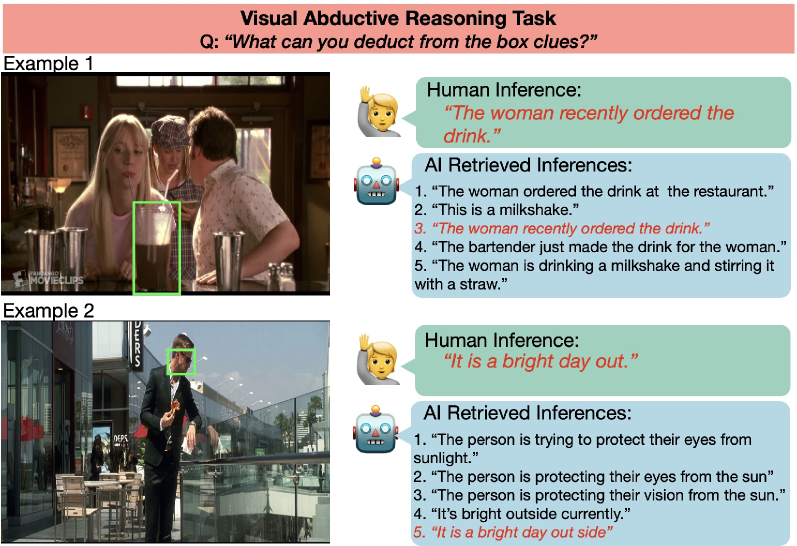
(a) Visual Abductive Reasoning Task

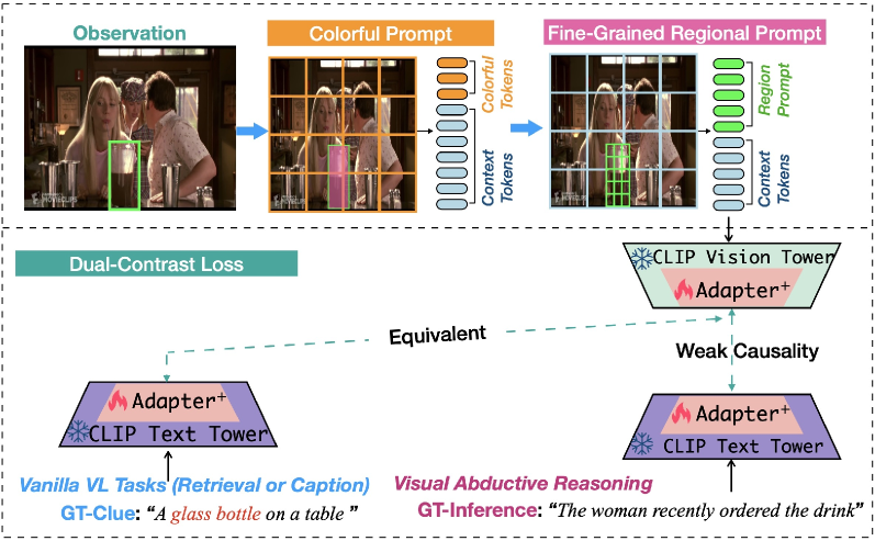
(b) Region-Prompted Adapter ( RPA)

Figure 1: Task of Visual Abductive Reasoning (VAR) and Methodology of Region-Prompted Adapter Tuning. (a). Given a pre-specified region of a picture (Example 1), human beings could easily reckon inference (e.g., “the woman recently ordered the drink”) from a local observation (e.g., “glass bottle”). To imitate humans, the VAR requires the AI to retrieve the most likely inferences for the same region; (b). The RPA first patchify regional observation at a more fine-grained level than its colorful counterpart (CPT), and then adjust the frozen CLIP with plugged Adapter${}^{\textbf{+}}$ for downstream tasks. The new Dual-Contrasive Loss simultaneously shrinks gaps between “Vision-Inference/-Clue” modalities. (This figure is best viewed in color)

“Can machines think?” Dr. Alan Turing proposed this question and gave the famous thought test, namely the “Imitation Game”, to help find an answer [1]. This game defines that we could consider “a machine thinks” if it fully imitates humans’ feedback and tricks us (humans) into believing its replies. Recent progress of foundation models, including GPT [2], and CLIP [3], shows that machines could imitate humans better than before, showing evolving thinking and reasoning abilities.

To promote machines’ reasoning ability, researchers devoted more and more efforts to reckon various modalities [4, 5, 6, 7, 8, 9]. One of the most challenging multimodal reasoning tasks is the Visual Abductive Reasoning (VAR)[5]. Specifically, the VAR aims to reveal a hidden inference or hypothesis from visual observations based on prior knowledge. As shown in Figure 1a, the machine is expected to draw an inference “the woman recently ordered the drink” from regional visual hints (“glass bottle”) and surrounding contexts ( “restaurant scene” + “waitress”), just as humans do.

However, the VAR task is more challenging than standard vision-language (VL) tasks (e.g., retrieval and captioning) [10, 11, 12, 13, 14, 15, 16, 17, 18]. The reasons lie in two aspects. Firstly, for the VAR, inferences are usually not readily apparent in images (e.g., “recently ordered drink” $\neq$ “glass bottle”, “restaurant” or “waitress”), whereas, for vanilla VL tasks, entities in captions appear in images (e.g., “glass bottle” in clue sentence “A glass bottle on a table”). Secondly, inferences have causal relations with the local visual hints. The presence or absence of evidential hints will result in different inferences (it’s hard to draw the inference “recently ordered drink” without seeing a glass bottle plus restaurant decoration).

The typical VAR pipeline contains two steps to reckon an inference from regional hints: Perception and Reasoning Tuning. The former step relies on pre-trained foundation models (e.g., CLIP) to provide prior knowledge and commonsense, transforming visual observations to semantical representation. The latter turns to specific prompt tuning to re-direct the model to align the transformed representation with the inference. Specifically, Colorful Prompt Tuning (CPT in Fig. 1b is adopted to preprocess images by covering the evidential visual part with a translucent pink box overlay. The altered images are then fed into the CLIP model to minimize the “vision-inference” gap through full fine-tuning.

Although effective, the pipeline has three limitations. First, CPT does not effectively extract fine details from the regional evidence. As shown in Figure 1b, the CPT uniformly patchify regional hints and global contexts at the same granularity. Even though the regional part is smaller than the global context in size, it has a more significant influence on the hypothesis. Thereby, uniformly patchifying on regional hints and global context may lead to losing fine-grained details in the regional evidence. Second, to steer the VLF for deduction, the existing pipeline fully fine-tunes all parameters using a limited amount of downstream data. However, this strategy can cause overfitting of the large VLF model, which could hamper its generalizability. The last is “How to utilize Triangular Relationships between Vision (visual evidence), Inference (hypothesis), and Clue (textual clue) for the VAR”. We argue that there is a weak causal relationship between “vision-inference” and a semantical relationship between “vision-clue” modalities. Current methods do not attempt to bridge these relations in a symmetric manner. We propose explicitly finding a correlation law among the three modalities and utilizing it to address the VAR task effectively.

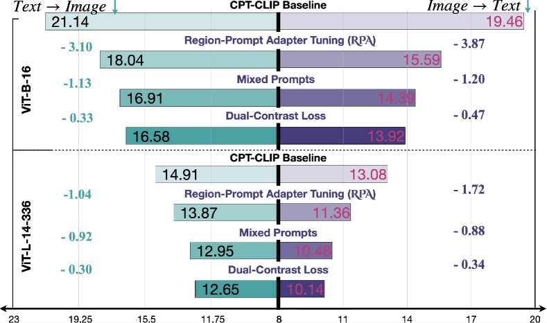
(a) Improvements of $Image$ $\leftrightarrows$ $Text$ Mean Rank (i.e., observation $\leftrightarrows$ hypothesis; lower=better)

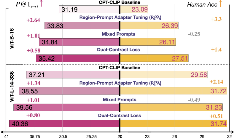
(b) Improvements of P@1_i→t and comparison with human (higher=better)

Figure 2: Performance boosts obtained by RPA Tuning and Dual-Contrastive Loss on the Sherlock testing set with two ViT backbone architectures. (This figure is best viewed in color)

To address the three limitations, we propose a new approach dubbed Region-Prompted Adapter Tuning ( RPA) combined with Dual-Contrastive Loss learning, which improves the current VAR pipeline (see Figure 3a). Within the RPA, there are two main components: fine-grained Regional Prompt Generator (RPG) and an enhanced Adapter${}^{\textbf{+}}$. Specifically, the RPG alleviates “loss in details” by gathering visual prompts from regional hints and global context at two levels of granularity (see Fig 1b). We pluck more tokens from regional hints using smaller patch sizes than those employed by CPT. We also sample surrounding tokens with the normal patch size to retain essential in-context information for inference reasoning. For implementation, We do not tweak the patch size in the embedding layer so as to reuse all the parameters in the CLIP. Alternatively, we turn to enlarge the area of the regional hint and then patchify it with the original embedding layer. For the second concern, we replace the full fine-tuning with Adapter${}^{\textbf{+}}$ tuning. The adapter tuning is a parameter-efficient fine-tuning (PEFT) initially designed for language models (LM) but recently expanded to VLFs. Our Adapter${}^{\textbf{+}}$ improves upon the basic adapter by introducing a new Map Adapter, which includes extra attention maps re-weighting using a low-rank query/key projection. For the last concern, we experimentally study different combinations of three contrastive losses (see Fig 5) and validate that the Dual-Contrasitive Loss, involving the loss of vanilla visual retrieval, benefits reasoning results. This also indicates that the VAR and visual retrieval tasks are positively correlated.

Experiments on the Sherlock VAR benchmark show that our model consistently surpasses previous SOTAs (Fig. 2), ranking the 1 on the leaderboard among all submissions . Our contributions are summarized below.

• Region-Prompted Adapter Tuning ( RPA). We introduce the RPA, the first hybrid Parameter-Efficient Fine-Tuning (PEFT) method within the “prompts + adapter” paradigm. It guides frozen Visual Language (VL) foundation models to make decisions based on local cues.

• Fine-Grained Region Prompts. We have designed a new visual prompt that encodes regional hints at a fine-grained level within the CLIP model. Our tests confirm that emphasizing local evidence improves visual reasoning.

• Enhanced Adapter${}^{\textbf{+}}$ Tuning. We present a new Map Adapter that adjusts the attention map using extra query/key projection. This adapter is orthogonal to the vanilla adapter, and they are jointly used to form the Adapter${}^{\textbf{+}}$.

• Dual-Contrastive Loss. We link the visual abductive reasoning and standard visual retrieval tasks using Dual-Contrastive Loss. Even though these two tasks have different “Vision-Text” relationships (causal vs semantical), we find that they are positively correlated and can be fine-tuned together.

• New State-of-the art for VAR. We evaluate RPA with Dual-Contrastive Loss on the standard Sherlock benchmark. Experiments show that our model robustly surpasses previous SOTAs, achieving a new record (e.g., Human Acc: RPA 31.74 vs CPT-CLIP 29.58).

II Related Works

Our Region-Prompted Adapter Tuning is relevant to research areas, including Foundation Models, Abductive Reasoning Tasks, Parameter-Efficient Fine-Tuning, and Fine-Grained Visual Representation. We will separately illustrate related works according to the areas below.

Foundation Models. “More is different” [19]. Scaling up models’ complexities and training data scales significantly improves the attention-based [20, 21, 22, 23] foundation models’ [2, 24, 3, 25, 26, 27] perception capacity, making it proficient in humanoid tasks such as zero or few-shot learning. Specifically, Large Language Models (LLM), such as BERT [24], and GPT [2] pre-trained on a large-scale corpus, are generalizable to downstream NLP tasks with few training examples. This trend quickly swept to the Vision-Language areas, with representative works such as CLIP [3], ALIGN [25], BLIP [28] etc. The main idea behind the VL foundation models is to learn transferable visual representation with noisy text supervision through a two-tower structure. We follow the current VAR pipeline and adopt the foundation model CLIP to generate initial visual & textual features.

Abductive Reasoning Tasks. Humans reckon plausible inferences or hypotheses from incomplete observations every day [29]. To teach the machine with this ability, researchers proposed several new Tasks, like ART [30] for NLP, Sherlock [5] for vision, and VideoVAR [6], VideoABC [7] for video. Specifically, the ART [30] generates the most likely hypothesis (text) to explain what has happened between the two observations (texts). For Sherlock, VideoVAR, and VideoABC, the observations are represented by regional or whole images, while inference could be text or middle frames. There are several similar tasks, such as Visual Commonsense Reasoning (VCR) [31] and Visual7W [32]. Abductive reasoning differs from them in having non-definitely correct, plausible inferences as human beings.

Parameter-Efficient Fine-Tuning (PEFT). Transferring foundational models to downstream tasks promotes the development of PEFTs [33]. Representative PEFTs include Prompt, Adapter, and LoRA tuning. Specifically, prompt tuning [2, 34, 35, 36, 37] enhances the distinctiveness of inputs by prepending additional tokens, which may be either trainable or fixed. The VL prompt tuning can further be divided into textual [38, 39, 40, 41] or visual prompt [42, 43] tuning, depending on the placement of prompt tokens in visual or textual encoders. Certain special visual prompts, such as the Merlot [44], CPT [45], and CiP [46], guide the model to focus on specified areas by overlaying these regions with translucent colors or red circles. In adapter tuning, trainable Multi-Layer Perceptron (mini MLP) [47, 48, 49] or Tiny Attention modules [50] are usually inserted into the foundational model, with only the new additions being fine-tuned. In the case of LoRA [51], model parameters are adjusted using low-rank projections. Our RPA belongs to a hybrid “prompt+adapter” tuning to equip the VLF with local reasoning ability, an approach that has not been studied before.

Fine-Grained Visual Representation. Our work is also relevant to learning fine-grained visual representation [52, 53, 54, 55, 56, 57] and object detection [58, 59, 60, 61, 62]. Specifically, GLIP [54] and RegionCLIP [52] pre-train foundation models for object detection, supervised by region-text pairs. The former and latter mimic the process of R-CNN[63] and Faster-RCNN [64], generating an object’s vector by either encoding the cropped image or RoI pooling. Similarly, UNITER [65] and LXMERT [66] also rely on RoI pooling to generate regional vectors for vanilla VL tasks. Besides, the InternImage [55] learns the foundation model with Deformable-CNN and achieves a new SOTA for object detection. Other works, such as Object-VLAD [53] for event detection, and CLIPTER [56] for scene text recognition, also studied fine-grained modeling. Specifically, the Object-VLAD aggregates densely collected local features with VLAD for generating video representation. The CLIPTER introduces extra cross-attention and the gated fusion module to combine local and global features. In contrast, our RPA doesn’t tweak the CLIP structure and only modifies the input space.

III Problem Definition & Baseline

Problem: Hessel et al.[5] defines a Visual Abductive Reasoning benchmark named “Sherlock” that requires a model to predict the hypothesis from observations in “Observation $\boldsymbol{\rightarrow}$ Hypothesis” form. Specifically, visual observation refers to a pre-specified region $\boldsymbol{r}$ of an image $\boldsymbol{i}$ and is accompanied by a clue sentence $\boldsymbol{c}$. Notably, the clue is a straightforward description of real visual content and is only available during training. On the other hand, the hypothesis is defined by an inference sentence $\boldsymbol{f}$. With this, a VAR model calculates a score $\boldsymbol{s}$, which reflects the probability of deducing inference $\boldsymbol{f}$ from the region $\boldsymbol{r}$. Equation 1 shows this scoring function $\mathcal{F}$ and the parameters $\theta$; we call $\mathcal{F}$ the VAR model.

$$s =\mathcal{F}(\boldsymbol{f},\boldsymbol{i},\boldsymbol{r}|\theta)$$ (1)

A good VAR model should generate a larger matching score when an inference $\boldsymbol{f}$ and observation $\{\boldsymbol{i}$, $\boldsymbol{r}\}$) are causally related, and a smaller value for wrong or non-related inferences.

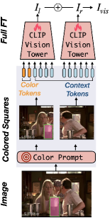
(a) CPT

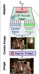
(b) RPA

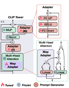
(c) RPA (Adapter${}^{\textbf{+}}$)

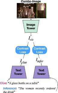
(d) Dual-Contrastive Loss

Figure 3: Comparing Colorful Prompt Tuning and Region-Prompted Adapter Tuning. (a) Colorful Prompt Tuning (CPT) from [45] uses a semi-transparent pink mask to highlight a designated area, marked as $\boldsymbol{r}$; (b) Our method, termed Region-Prompted Adapter Tuning ( RPA), simultaneously generates region prompt and contextual tokens by intaking a combo-image $\boldsymbol{J}$, then tunes the frozen CLIP with Adapter${}^{\textbf{+}}$ on top of reasoning dataset; (c) Adapter${}^{\textbf{+}}$ includes two standard adapters and a novel Map Adapter, which separately adjust token features and the attention map; (d) Dual-Contrastive Loss simultaneously guide the visual content minimize semantic (to clue) and causal (to inference) gaps. (Note: Best viewed in color.)

Baseline: As presented in [5], a CLIP [3] with colorful prompt tuning (CPT) [45] is adopted as the baseline for the Sherlock benchmark (Fig. 3a). Specifically, the CPT highlights the regional observation $\boldsymbol{r}$ by a translucent pink overlay (or mask). Then the altered image $\boldsymbol{i}$ is split into left & right parts (i.e., $\boldsymbol{i}_{l}$ & $\boldsymbol{i}_{r}$) for feature extraction (Eq. 2), and the global feature $\mathcal{I}_{vis}$ is averaged from both parts (Eq. 3). Meanwhile, the inference text $\boldsymbol{f}$ is encoded into a textual feature vector $\mathcal{I}_{text}$ by a text encoder $\mathcal{F}_{\text{T}}$ (Eq. 4). To reduce overfitting, the inference text $\boldsymbol{f}$ is randomly replaced by the clue $\boldsymbol{c}$ with a probability of 0.5 during training. This strategy is named Multi-Task Learning as now the model has to predict inference text 50% of the time and clue text 50% of the time during training. Finally, a contrastive loss $\mathcal{L}_{ctr}$ bridges the gap between visual and textual features as shown in Eq. 5.

$$\mathcal{I}_{l}=\mathcal{F}_{\text{V}}(\boldsymbol{i}_{l}),~{}~{}~{}\mathcal{I}_{r}=\mathcal{F}_{\text{V}}(\boldsymbol{i}_{r})$$ (2)

$$\mathcal{I}_{vis}=\left(\mathcal{I}_{l}+\mathcal{I}_{r}\right)/2$$ (3)

$$\mathcal{I}_{text}=\left\{\begin{aligned} \mathcal{F}_{\text{T}}\left(\boldsymbol{f}\right)&,p\geqslant 0.5&\\ \mathcal{F}_{\text{T}}\left(\boldsymbol{c}\right)&,p<0.5&\end{aligned}\right.$$ (4)

$$loss=\mathcal{L}_{ctr}\left(\mathcal{I}_{vis},\mathcal{I}_{text}\right)$$ (5)

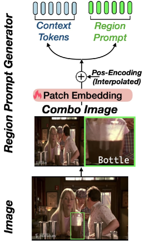
(a) R-CTX

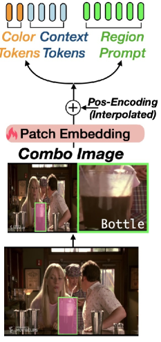
(b) R-CPT

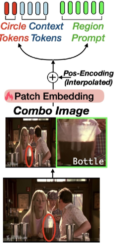
(c) R-CiR

Figure 4: Three Types of Fine-Grained Region Prompts generated by the Regional Prompt Generator. In RPG, we assemble the combo-image $\boldsymbol{J}$ from region $\boldsymbol{r}$ and context, colorful, or circle-prompted image $\boldsymbol{i}$. Then, the combo-image $\boldsymbol{J}$ goes through the patch-embedding layer and is further added with positional embedding to generate input tokens. (a) R-CTX: Region+Context; (b) R-CPT: Region+Colorful Prompt; (c) R-CiP: Region+Circle Prompt.

IV Method

In this section, we introduce our Region-Prompted Adapter Tuning ( RPA in Fig. 3b), which enhances the frozen VL foundation models to focus on specific visual cues for deducing inference. The RPA consists of two main parts: a Regional Prompt Generator (RPG in §IV-A) for targeting specific visual areas and an Adapter${}^{\textbf{+}}$ module (§IV-B) to transfer the frozen CLIP model for reasoning tasks. Finally, we replace Multi-Task Learning [5] with a new Dual-Contrastive Loss (§IV-C) to bring the visual features closer to both literal description (“clue”) and hypothesis (“Inference”). We will elaborate on each section below.

IV-A Regional Prompt Generator

We propose treating pre-specified observation $\boldsymbol{r}$ as a “prompt” to directly guide the visual reasoning process. Our Regional Prompt Generator (RPG) can create three detailed prompts focusing on specific areas. These prompts harness local features (i.e., region), surrounding context, and existing visual prompts as shown in Figure 4a-4c. All three types of prompts go through the same process, with the only difference in being whether colors or circles are drawn on the input images. To explain how it works, we’ll use the “Region+Context” (R-CTX) as an example.

To prepare prompt and contextual tokens, we pop out patch-embedding layer $\mathcal{F}_{proj}$ and positional encoding PE from the vision tower $\mathcal{F}_{\text{V}}$. We further resize region $\boldsymbol{r}$ and full image $\boldsymbol{i}$ into squares of the same size, then concatenate them vertically (or horizontally) into a combo-image $\boldsymbol{J}$ (Eq. 6). We apply patch-embedding on the combo and add it with upsampled PE_inter to get visual tokens $\boldsymbol{z}_{0}$ (Eq. 7). As the PE_inter is twice the size of PE, we initialize it by inflating PE using bilinear interpolation. Notably, $\boldsymbol{z}_{0}$, generated from the combo-image, already includes both regional prompt and global contextual tokens. The $\boldsymbol{z}_{0}$ is further fed into the remaining attention and MLP layers (denoted by $\hat{\mathcal{F}}_{\text{V}}$) to get visual representation $\mathcal{I}_{vis}$ (Eq. 8). We unfreeze patch-embedding $\mathcal{F}_{proj}$ and positional encoding PE_inter to generate learnable soft prompts.

$$\boldsymbol{J}=Concat\left(\begin{bmatrix}\boldsymbol{r}\\ \boldsymbol{i}\end{bmatrix}\right)$$ (6)

$$\boldsymbol{z}_{0}=\mathcal{F}_{proj}(\boldsymbol{J})+\texttt{PE}_{inter}$$ (7)

$$\mathcal{I}_{vis}=\hat{\mathcal{F}}_{\text{V}}\left(\boldsymbol{z}_{0}\right)$$ (8)

For the “Region + Colorful Prompt” and “Region + Circle Prompt” (R-CPT & R-CiR), we create the combo-image $\boldsymbol{J}$ from the squared region $\boldsymbol{r}$ and a modified image $\boldsymbol{i}^{\prime}$. In this image $\boldsymbol{i}^{\prime}$, we either color the pixels inside the region with a translucent pink rectangle or outline them with a red circle.

Mixed Prompts: During training, we randomly choose from the three types of prompts (R-CTX, R-CPT, and R-CiR) with equal chance. For testing, we take the average of the visual representations created by these three prompts. For the text-based representation $\mathcal{I}_{text}$ and the loss function, we replace the equations 4-5 by the new equations 15-16 under the Dual-Contrastive Loss learning scheme. We’ll go into more detail about this loss in §IV-C.

IV-B Adapter${}^{\textbf{+}}$ Tuning

Adapter tuning adjusts a “locked-in” foundational model for downstream tasks by fine-tuning a few newly implanted modules. This method has successively swept over NLP [47] and computer vision [3] areas. Current adapter structures, like mini MLP and tiny attention modules, focus mainly on refining visual features. However, they don’t consider the need to adjust the original attention maps of the base models. To tackle this, we augment the vanilla adapter with a new, orthogonal Map Adapter, which precisely adapts attention maps in Transformers. This results in the improved Adapter${}^{\textbf{+}}$.

The Adapter${}^{\textbf{+}}$ pipeline is illustrated in Figure 3c. We first include two basic adapters, referred to as Adapter (A&M). They are placed after the MSHA module and parallel to the MLP module in the $l$-th encoder of a CLIP tower (e.g., $\mathcal{F}_{\text{V}}$ or $\mathcal{F}_{\text{T}}$). These adapters are shallow and contain only two fully-connected layers to downgrade and upgrade feature dimension ($\mathbb{R}^{D}\leftrightarrows\mathbb{R}^{d}$, $d<D$) with a GELU activation in between (Equation 9-11). The light red font indicates the tunable status of each layer.

$$\boldsymbol{z^{\prime}}_{l}={\text{MH}}{\text{SA}}\left(\boldsymbol{z}_{l-1}\right),~{}~{}~{}~{}~{}~{}~{}~{}~{}~{}~{}~{}~{}~{}~{}l=1,2,\cdots,L$$ (9)

$$\boldsymbol{z^{\prime\prime}}_{l}={\color[rgb]{.75,0,.25}\text{Adapter\_A}}\left(\boldsymbol{z^{\prime}}_{l}\right)+\boldsymbol{z}_{l-1},$$ (10)

$$\boldsymbol{z}_{l}={\text{MLP}}\left(\boldsymbol{z^{\prime\prime}}_{l}\right)+{\color[rgb]{.75,0,.25}\text{Adapter\_M}}\left(\boldsymbol{z^{\prime\prime}}_{l}\right)+\boldsymbol{z^{\prime\prime}}_{l},$$ (11)

The Map Adapter further refines the MSHA module by adding a small, modified attention map, labeled as $\widehat{\boldsymbol{Q}}\widehat{\boldsymbol{K}}^{T}$ (refer to Equation 12). This additive map helps to adjust the original attention map dynamically, improving the model’s ability to focus on relevant information. To ensure that the original attention map isn’t altered too much, we use simpler $D\rightarrow d$ projections for generating the query and key (see Equation 3). Here, $d$ is smaller than $D$.

$$\boldsymbol{z^{\prime}}_{l}={\text{Softmax}}\left(\frac{\boldsymbol{Q}\boldsymbol{K}^{T}+{\color[rgb]{.75,0,.25}\boldsymbol{\widehat{Q}}\boldsymbol{\widehat{K}}^{T}}}{{\sqrt{D}}}\right)\boldsymbol{V},$$ (12)

$${\color[rgb]{.75,0,.25}\boldsymbol{\widehat{Q}},\boldsymbol{\widehat{K}}}~{}=\boldsymbol{z}_{l-1}\times{\color[rgb]{.75,0,.25}\boldsymbol{\widehat{W}}_{q},\boldsymbol{\widehat{W}}_{k}},~{}~{}~{}{\color[rgb]{.75,0,.25}\widehat{\boldsymbol{W}}_{q,k}}\in\mathbb{R}^{D\times d}$$ (13)

$$\boldsymbol{Q},\boldsymbol{K},\boldsymbol{V}=\boldsymbol{z}_{l-1}\times\boldsymbol{W}_{q},\boldsymbol{W}_{k},\boldsymbol{W}_{v},\boldsymbol{W}_{q,k,v}\in\mathbb{R}^{D\times D}$$ (14)

We compared the enhanced Adapter${}^{\textbf{+}}$ with vanilla and Tiny Adapter counterparts (see §V-D) and found that our tuning method consistently performs better.

IV-C Dual-Contrastive Loss

As an observation contains three modalities, such as visual $\boldsymbol{J}$, clue sentence $\boldsymbol{c}$, and inference sentence $\boldsymbol{f}$, we comprehensively study their mutual influences by deploying contrastive loss between different modalities pairs. Specifically, as shown in Figure 5, we deploy dual, triple, and single contrastive loss in the training phase and screen out that the Dual-Contrastive Loss works best (Fig. 3d). We first elaborate on the Dual-Contrastive Loss and then compare it with the other counterparts.

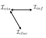
(a) $\mathit{Dual}$

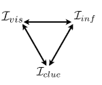
(b) $\mathit{Triple}$

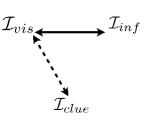
(c) $\mathit{Single}_{1}$

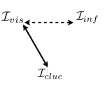
(d) $\mathit{Single}_{2}$

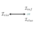
(e) $\mathit{MTL}$

Figure 5: Training Losses: Dual (a), Triple (b) and Single (c)-(e) contrastive loss for learning to match visual $\boldsymbol{J}$ to texts $\boldsymbol{c}$ and $\boldsymbol{f}$. Solid and dashed lines represent the presence or absence of contrastive loss during training.

Dual-Contrastive Loss: Both the clue $\boldsymbol{c}$ and inference $\boldsymbol{f}$ are positively relevant to visual $\boldsymbol{J}$. More specifically, the former is literally equivalent, while the latter is causally related to the visual hints. Although their relations are in different forms, we can still deploy a Dual-Contrastive Loss, including one for “vision-clue” pair and the other for “vision-inference” pair (Fig. 5a), to regress visual features toward two textual targets. The mathematical process is present in Equation 15-16.

$$\mathcal{I}_{inf}=\mathcal{F}_{\text{T}}\left(\boldsymbol{f}\right),~{}~{}\mathcal{I}_{clue} =\mathcal{F}_{\text{T}}\left(\boldsymbol{c}\right)$$ (15)

$$loss=\mathcal{L}_{ctr}\left(\mathcal{I}_{vis},\mathcal{I}_{clue}\right)+ \mathcal{L}_{ctr}\left(\mathcal{I}_{vis},\mathcal{I}_{inf}\right)$$ (16)

Other Loss Variants. The rest loss functions include the Triple and Single contrastive loss. Particularly, compared with dual contrastive loss, the triple one newly adds the “inference-clue” pair (e.g., Fig. 5b and Eq. 17).

$$loss=\mathcal{L}_{ctr}\left(\mathcal{I}_{vis},\mathcal{I}_{clue}\right)+ \mathcal{L}_{ctr}\left(\mathcal{I}_{vis},\mathcal{I}_{inf}\right)$$

$$+\mathcal{L}_{ctr}\left(\mathcal{I}_{inf},\mathcal{I}_{clue}\right)$$ (17)

We later observed that: additional inference-clue loss in triple contrastive hurts overall performance, as the two texts (i.e., clue and inference) are not literally equivalent. For example, the clue sentence “the road is wet”$\neq$ inference sentence “it has rained before”. Therefore, we can only let the two texts learn toward the same third-party feature (e.g., the visual) instead of artificially forcing them to be equivalent.

For the single contrastive loss, we have three options, namely vision-inference (Fig. 5c), vision-clue (Fig. 5d), multi-task learning (MTL in Fig.5e). Notably, we use an identical textual encoder for clue and inference during testing, since we only learn a single contrastive loss between a pair of modalities during training.

These three options can be expressed in one unified form (Eq. 18), by thresholding a random probability $p$ with different values $\overline{\mathrm{T}}$. Specifically, when $\overline{\mathrm{T}}=1.0~{}\mathrm{or}~{}0~{}\mathrm{or}~{}0.5$, the single contrastive loss degenerates into the vision-clue, vision-inference and multi-task learning loss.

$$\mathit{loss}=\mathcal{L}_{ctr}\left(\mathcal{I}_{vis},\mathcal{I}_{txt}\right),\mathcal{I}_{txt}=\left\{\begin{aligned} \mathcal{F}_{\text{T}}\left(\boldsymbol{f}\right)&,p>\overline{\mathrm{T}}&\\ \mathcal{F}_{\text{T}}\left(\boldsymbol{c}\right)&,p<\overline{\mathrm{T}}&\end{aligned}\right.$$ (18)

With the single contrastive loss, we find that only minimizing the gap between a pair, such as vision-clue (or vision-inference) will also shorten the gap between the other pair vision-inference (or vision-clue), indicating retrieval and abductive reasoning tasks have positive rational correlations. We give detailed analysis in §V-D.

V Experiments

We comprehensively study the RPA and Dual-Contrastive Loss on the Sherlock benchmark [5]. We also tested the RPA’s adaptability on the RefCOCO [67], which focuses on grounding expression to regions. The details of our experiments are provided below.

V-A Datasets

The Sherlock dataset [5] contains 103K images collected from the Visual Genome [68] and Visual Common Sense Reasoning [31] datasets. These images are split into 90K training, 6.6K validation, and 6.6K testing sets. Each image is re-annotated with an average of 3.5 observation-inference pairs, forming 363K samples. Particularly, a sample includes a bounding box $\boldsymbol{r}$ and two texts (i.e., clue $\boldsymbol{c}$ + inference $\boldsymbol{f}$). Notably, the validation set can be evaluated offline with officially provided scripts, while the testing set needs to be assessed online with the leaderboard.

Three types of evaluation metrics, from retrieval, localization, and comparision aspects, are adopted for the Sherlock benchmark. Specifically, retrieval metrics, such as $img\leftrightarrows text$ mean rank, P@1_i→t, are used to measure correspondence between visual fact and inference text. For localization, accuracies of grounding candidate regions to the inferences are adopted. The candidates can be collected from ground-truth or auto-detected boxes. Comparison metric calculates the accordance between machine and human predictions.

The RefCOCO dataset [67] originates from the MSCOCO dataset [69]. We test the generalization of the RPA on the Referring Expression Comprehension (REC task) using Accuracy@0.5. This task aims to link a distinctive sentence to a specific object box when multiple similar objects are present. A box aligned by a grounding sentence is considered correct if it has an Intersection over Union (IoU) of 0.5 with the ground-truth bounding box. This dataset contains 3 splits: RefCOCO, RefCOCO+, and RefCOCOg. The RefCOCO and RefCOCOg allow for relational expressions of position (left/right), while RefCOCO+ has only expression on appearance. Specifically, RefCOCO/+/g contains 19.9/19.9/26.7K images, respectively, covering 50.0/49.8/54.8K object instances with corresponding 142/141/85K referring expressions. Since REC requires bounding box proposals for the “text-to-region” grounding, we adopt the YoloV8 to generate candidate proposals as inputs for our RPA.

V-B Implementations

We develop the RPA and Dual Contrastive Loss on top of the OpenCLIP [3, 70] PyTorch toolkit, and fix the training & testing recipe to be the same for all ablations unless otherwise stated.

Training. We resize $\boldsymbol{r}$ and $\boldsymbol{i}$ into 224$\times$224 (336 for high resolution) square images and further concatenate them into combo-image $\boldsymbol{J}$ of size 448$\times$224. We initialize CLIP from OpenAI pre-trained weight and tuning for 10 epochs with a cosine learning rate schedule. Thanks to mixed-precision and gradient-checkpointing [71], we train with a global batch size=3200, lr=2e-4 using CLIP ViT-B-16 backbone (batch=400, lr=2e-5 for ViT-L-14-336) on 2$\times$80 GB A100 GPUs.

Testing. We apply the same preprocess for region $\boldsymbol{r}$ and full image $\boldsymbol{i}$ to prepare regional prompt and contextual token as the training phase. Given a set of visuals $\{\boldsymbol{r}$, $\boldsymbol{i}\}\times K$ and inferences $\{f\}\times K$, we first calculate the $K\times K$ matrix of vision-inference similarity and report retrieval, localization and comparison metrics based on the matrix.

TABLE I: Comparison with state-of-the-art methods using the Sherlock Testing Leaderboard.
(The up arrow $\uparrow$ (or down arrow $\downarrow$) indicates the higher (or lower), the better.)

Test-Set		Parameters	Retrieval			Localization	Comparison
Model	Backbone	Tuned (M$\downarrow$)	im$\rightarrow$txt ($\downarrow$)	txt$\rightarrow$im ($\downarrow$)	P@1i→t ($\uparrow$)	GT/Auto-Box ($\uparrow$)	Human Acc ($\uparrow$)
LXMERT [66] from [5]	F-RCNN	NA	51.10	48.80	14.90	69.50 / 30.30	21.10
UNITER [65] from [5]		NA	40.40	40.00	19.80	73.00 / 33.30	22.90
CPT [45] from [5]	RN50$\times$64	NA	16.35	17.72	33.44	87.22 / 40.60	27.12
CPT [45] from [5]		149.62	19.85	21.64	30.56	85.33 / 38.60	21.31
CPT [45] (our impl)		149.77	19.46	21.14	31.19	85.00 / 38.84	23.09
Full Fine-Tuning (R-CTX)		149.77	15.63	18.20	33.76	86.19 / 40.78	27.32
Our RPA (R-CTX)	ViT-B-16	42.26	15.59	18.04	33.83	86.36 / 40.79	26.39
$\Lsh$ Mixed Prompts		42.26	14.39	16.91	34.84	87.73 / 41.64	26.11
$\Lsh$ Dual-Contrast Loss		42.26	13.92	16.58	35.42	88.08 / 42.32	27.51
CPT [45] (our impl)		428.53	13.08	14.91	37.21	87.85 / 41.99	29.58
Our RPA (R-CTX)	ViT-L-14	89.63	11.36	13.87	38.55	88.68 / 42.30	31.72
$\Lsh$ Mixed Prompts	(336)	89.63	10.48	12.95	39.68	89.66 / 43.61	31.23
$\Lsh$ Dual-Contrast Loss		89.63	10.14	12.65	40.36	89.72 / 44.73	31.74

TABLE II: Comparison with state-of-the-art methods using the Sherlock Testing Leaderboard.

Val-Set	Parameters	Retrieval			Localization	Comparison
Model	Tuned (M$\downarrow$)	im$\rightarrow$txt ($\downarrow$)	txt$\rightarrow$im ($\downarrow$)	P@1i→t ($\uparrow$)	GT/Auto-Box ($\uparrow$)	Human Acc ($\uparrow$)
CPT [45] (our impl)	149.77	19.03	20.66	31.10	85.05 / 38.37	25.07
$\Lsh$ Adapter${}^{\textbf{+}}$ + Dual-Contrast Loss	149.77	17.99 (-1.04)	19.71 (-0.95)	31.94 (+0.84)	86.22 / 39.98 (+1.17 / 1.61)	25.53 (+0.46)
Our RPA (R-CTX)	42.26	16.30	17.92	33.09	86.10 / 40.80	25.83
$\Lsh$ Mixed Prompts	42.26	15.16 (-1.14)	16.96 (-0.96)	34.57 (+1.48)	87.96 / 41.60 (+1.86 / 0.80)	25.64 (-0.19)
$\Lsh$ Dual-Contrast Loss	42.26	14.26 (-0.90)	16.44 (-0.52)	35.46 (+0.89)	88.23 / 41.91 (+0.27 / 0.31)	26.80 (+1.16)

V-C Comparision with the State-of-the-Art

We compare RPA with the current state-of-the-art on the Sherlock test set. All results are submitted, evaluated, and published on the official leaderboards. We didn’t test RPA with CLIP ResNet50$\times$64 backbone, as Adapter⁺ is presently designed for Transformers.

As shown in Table I, our top-performing RPA ranks the 1 on the Sherlock Leaderboard across most of the evaluation metrics. It significantly outperforms competitors like CPT-CLIP, UNITER, and LXMERT. For example, our model achieves a “Human Acc” score of 31.74, compared to 29.58, 22.90, and 21.10 for the other models. We note that models built on the CLIP framework, including ours, perform much better than traditional models like UNITER and LXMERT. This suggests that large-scale pre-trained knowledge is beneficial for tasks requiring abductive reasoning. We further validated that our RPA performs well with fine-grained regional evidence as a prompt for visual reasoning tasks. Our model achieves a Human Acc score of 26.39/31.74 ($\uparrow$3.30/2.16), compared to 23.09/29.58 for CPT-CLIP when using different backbones. Lastly, our new “Dual-Contrastive Loss” feature further enhances the performance of the RPA. This performance improvement is consistent across other test data (val-set in Table II) and backbones (i.e., ViT-B-16/ViT-L-14), indicating its robustness. In summary, our model with Dual-Contrastive Loss outperforms current state-of-the-art methods.

TABLE III: Impacts of integrating adapters. We compare the single, dual, and triple adapters.

Val-Set	Adapter Types			Parameters	Retrieval			Localization	Comparison
Adapters	Adapter_M	Adapter_A	Map Adapter	Tuned (M$\downarrow$)	im$\rightarrow$txt ($\downarrow$)	txt$\rightarrow$im ($\downarrow$)	P@1i→t ($\uparrow$)	GT/Auto-Box ($\uparrow$)	Human Acc ($\uparrow$)
$\Lsh$ $\times 1$			✓	32.00	19.35	22.56	30.46	85.77 / 39.27	22.89
$\Lsh$ $\times 1$		✓		32.01	18.52	21.53	31.40	85.85 / 39.29	23.63
$\Lsh$ $\times 1$	✓			32.01	14.79	17.14	34.82	87.82 / 42.32	26.66
$\Lsh$ $\times 2$		✓	✓	37.13	16.41	18.98	33.11	86.96 / 40.28	24.99
$\Lsh$ $\times 2$	✓	✓		37.14	14.75	16.76	35.14	87.89 / 41.08	26.78
$\Lsh$ $\times 2$	✓		✓	37.13	14.51	16.54	35.15	88.06 / 41.34	26.41
RPA   $\Lsh$ $\times 3$	✓	✓	✓	42.26	14.26	16.44	35.46	88.23 / 41.91	26.80

TABLE IV: Impacts of Fine-Grained Regional Prompts.

Val-Set	Retrieval			Localization	Comparison
Prompt Type	im$\rightarrow$txt ($\downarrow$)	txt$\rightarrow$im ($\downarrow$)	P@1i→t ($\uparrow$)	GT/Auto-Box ($\uparrow$)	Human Acc ($\uparrow$)
Region Only	22.76	22.62	30.44	86.10 / 41.86	23.66
Context	45.28	54.57	18.12	NA	21.99
$\Lsh$ + Region (R-CTX)	15.24 (-30.04)	17.22 (-37.35)	34.29 (+15.88)	87.23 / 41.11	26.69 (+4.70)
CPT [45]	17.99	19.71	31.94	86.22 / 39.98	25.53
$\Lsh$ + Region (R-CPT)	14.30 (-3.69)	16.17 (-3.54)	35.57 (+3.63)	87.91 / 42.18 (+1.69 / 2.22)	26.21 (+0.68)
CiP [46]	18.08	19.89	31.71	85.85 / 39.99	24.11
$\Lsh$ + Region (R-CiP)	14.27 (-3.81)	16.25 (-3.64)	35.61 (+3.90)	87.90 / 42.62 (+2.05 / 2.63)	26.51 (+2.40)
Mixed Prompts ( RPA)	14.26	16.44	35.46	88.23 / 41.91	26.80

V-D Ablation Study

This section comprehensively studies various factors that influence the performance of our model on the validation set. We examine different integrations of Adapters and Regional Prompts, various contrastive losses, the impact of the bottleneck dimension $d$ in Adapters, and the effect of using different backbones and resolutions. For these tests, we use Mixed Prompts, Dual-Contrastive Loss and ViT-B-16 as our default settings, except in the ablations where we compare the performance of different prompts, losses or backbones.

Impacts of Integrating Adapters. We analyze how our model performs when we remove certain components, specifically the vanilla (A&M) and Map Adapters, one at a time. The results in Table 3 show that performance decreases with fewer adapters. Specifically, using all three types of adapters produces the best results under most evaluation metrics. “Adapter (M)” is the best choice when limited to using just one type of adapter. If we can use two types, the best combination is “Adapter (M) + Map Adapter”, suggesting that the Map Adapter complements the vanilla adapter well.

Effects of Fine-Grained Regional Prompts. We also explore how adding fine-grained regional prompts influences the performance of existing prompting techniques, such as colorful (CPT in [45]) and circle prompts (CiP in [46]). In Table IV, the terms “Region Only” and “Context” refer to feeding either just the regional box part or the entire image into the CLIP vision tower, respectively.

We observe that adding fine-grained tokens based on regional cues significantly improves the performance of all coarse-grained prompts, including “Context”, “CPT”, and “CiP” across all metrics. This basically verifies that “global context + local cues” complement each other well for abductive reasoning. Moreover, we test the Mixed Prompt mode described in §IV-A and observe a stable performance for most metrics.

Dual-Contrastive Loss vs Single/Triple counterparts. We test different types of contrastive losses using our RPA model. In Table V, the Dual-Contrastive loss performs better than the Multi-Task Learning and the other single & triple counterparts under most metrics. In terms of localization, the Dual-Contrastive loss is slightly lower than its MTL counterparts but still shows a very competing performance.

TABLE V: Comparison of Different Learning Losses on Sherlock Validation Set.

Val-Set	Retrieval			Localization	Comparison
Loss Type	im$\rightarrow$txt ($\downarrow$)	txt$\rightarrow$im ($\downarrow$)	P@1i→t ($\uparrow$)	GT/Auto-Box ($\uparrow$)	Human Acc ($\uparrow$)
Clue-Image Contrast	36.36	49.98	25.29	82.52 / 30.23	21.64
Inference-Image Contrast	15.16	16.96	34.57	87.96 / 41.60	25.64
Multi-Task Learning [5]	14.75	16.92	34.82	87.63 / 42.33	26.07
Triple-Contrast	14.75	16.90	35.40	88.22 / 41.91	25.31
Dual-Contrast ( RPA)	14.26	16.44	35.46	88.23 / 41.91	26.80

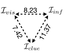
(a) $\mathit{NoTrain}$

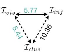
(b) $\mathit{Single}_{1}$

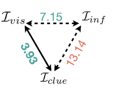
(c) $\mathit{Single}_{2}$

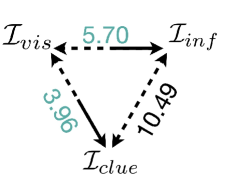
(d) $\mathit{MKL}$

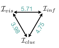
(e) $\mathit{Triple}$

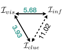
(f) $\mathit{Dual}$

Figure 6: Individual Contrastive Loss between Modality Pair on Sherlock Validation Set. We used a model trained with (a) No Training, (b-c) Single, (d) MKL, (e) Triple, and Dual (f) losses. The Green/Red implies the significantly decreasing/increasing of loss values, compared with No Training. Solid and dashed lines represent the presence or absence of contrastive loss during training.

We further look into the individual contrastive loss value between modality pairs on the validation set to understand how modalities mutually influence each other. Specifically, we first report the loss value between each pair before the training phase (i.e., No Train or Zero-Shot reasoning), then re-calculate them after the model is trained with different losses (Fig 6).

We observe that the gaps of vision-clue and vision-inference are positively correlated. Specifically, when we minimize one of the gaps in training, the other one will also become smaller (e.g., Fig. 6b-6c). Whereas, the gap of inference-clue seems not to correlate to gaps of vision-clue and -inference, as the former is slightly closer or even larger after minimizing either of the latter gaps (e.g., red/black value in Fig 6b-6d, and 6f). If we enforce the model to close the inference-clue gap during training, the vision-clue and -inference gap would become larger (Triple vs Dual, Fig. 6e vs 6f). The reason is that the clue and inference sentences are not literally equivalent and better to be bridged by an extra rational process.

Influence of Bottleneck Dimension $d$ in Adapters. We study the influence of different bottleneck dimensions in the RPA, ranging in $d=\{\frac{D}{32},\frac{D}{16},\frac{D}{8},\frac{D}{4},\frac{D}{2},D\}$. Notably, a higher $d$ basically introduced more tuned parameters and larger FLOPs, as shown in Figure 7a. For the retrieval metrics, such as mean $img\leftrightarrows txt$ rank, a lower value indicates better performance, whereas the rest are the opposite. We observe from Figure 7b-7e that an optimal choice is $d=\frac{D}{4}$, indicating that adjusts the frozen foundational model with either a very heavy $D$ or lightweight $\frac{D}{32}$ would result in sub-optimal performance. Notably, human accordance is influenced by the human’s subjective judgment and has a different trend. Overall, we fix $d=\frac{D}{4}$ for all following experiments.

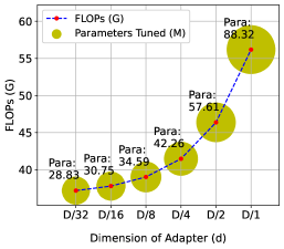
(a) FLOPs and Tuned Params ($\downarrow$)

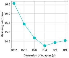
(b) Mean ${img\rightarrow txt}$ Rank ($\downarrow$)

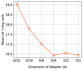
(c) Mean ${txt\rightarrow img}$ Rank ($\downarrow$)

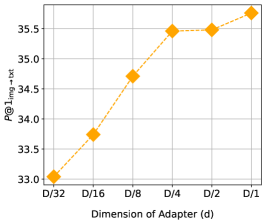
(d) Retrieval P@1_img→txt ($\uparrow$)

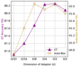
(e) Localization ($\uparrow$)

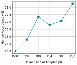
(f) Human Accordance ($\uparrow$)

Figure 7: Performance comparison of different bottleneck dimensions in adapters ($d$). The direction of $\downarrow$ or $\uparrow$ indicates the lower/higher of the value, the better the performance is. Best viewed in color.

Comparison with tiny attention counterpart [50]. As in Table VI, we compare the performances between different integrations of “TinyAtten + Adapter$\_$M / Adapters$\_$(A & M)” (Figure 8) against RPA (Figure 3c) on frozen CLIP ViT-B-16. We note that “TinyAtten + Adapters$\_$(A&M)” performs worse than the RPA with more tuned parameters and FLOPs. The reason might be Map Adapter only re-weights the attention map and does not change the “value” bases. Overall, the RPA is a more effective and efficient adapter than its counterparts.

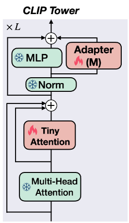
(a)

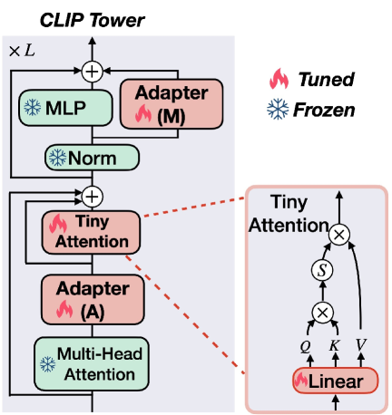
(b)

Figure 8: Tiny Attention Counterparts. (a): TinyAtten + Adapter_M; (b): TinyAtten + Adapter_A&M

TABLE VI: Comparison of Map Augmented Adapter and Tiny Attention Adapter

Val-Set	FLOPs	Parameters	Retrieval			Localization	Comparison
Attention Adapter	(G$\downarrow$)	Tuned (M$\downarrow$)	im$\rightarrow$txt ($\downarrow$)	txt$\rightarrow$im ($\downarrow$)	P@1i→t ($\uparrow$)	GT/Auto-Box ($\uparrow$)	Human Acc ($\uparrow$)
Tiny Atten + Adapter$\_$M	41.82	42.26	14.91	17.17	34.33	87.87 / 42.18	26.03
Tiny Atten + Adapter$\_$(A & M)	43.33	47.39	14.68	16.74	34.90	87.68 / 41.91	25.46
Map Adapter + Adapter$\_$(A & M)	41.48	42.26	14.26	16.44	35.46	88.23 / 41.91	26.80

Influence of Adapting CLIP Vision/Text Tower. The CLIP follows a two-tower design, each tower separately for visual/textual embedding; thereby, we can independently insert adapters into visual and textual towers to assess their contributions. We test inserting Adapter${}^{\textbf{+}}$ into the “Only Text” tower, “Only Vision” tower, and both towers. As shown in Table VII, adapting both CLIP vision and text towers performs the best at the cost of the most tuned parameters among the three options. Notably, both “Only Vision” and “Only Text” has a large margin in performance compared with the “Vision + Text”, indicating the adaptions on two towers are complementary.

TABLE VII: Influence of Adapting CLIP Vision/Text Tower.

Val-Set	Parameters	Retrieval			Localization	Comparison
Towers	Tuned (M$\downarrow$)	im$\rightarrow$txt ($\downarrow$)	txt$\rightarrow$im ($\downarrow$)	P@1i→t ($\uparrow$)	GT/Auto-Box ($\uparrow$)	Human Acc ($\uparrow$)
Only Text Adapter${}^{\textbf{+}}$	31.62	29.57	34.37	25.72	77.71 / 34.08	20.67
Only Vision Adapter${}^{\textbf{+}}$	37.53	19.02	21.18	31.79	86.93 / 40.38	24.02
Vision + Text Adapter${}^{\textbf{+}}$s	42.26	14.26	16.44	35.46	88.23 / 41.91	26.80

Influence of Image Resolutions. We test combo images with different resolutions to study whether the RPA can benefit from more tokens. As in Table VIII, it is natural to see an increment of computations when resolutions become larger. However, the boost of performance is not linear to the resolutions, reaching a saturate performance at the resolution of 448$\times$224. This might lie in that the CLIP is pre-trained at 224$\times$224 resolution on upstream dataset, thereby, downstream tuning is better to process images (one 448$\times$224 combo image = two 224$\times$224 images) at similar settings. Considering the trade-off of FLOPs and performance, we pick the resolution of 448$\times$224 for the CLIP ViT-B-16 backbone.

TABLE VIII: Impact of input image resolution on the performance.

Val-Set	FLOPs	Retrieval			Localization	Comparison
Resolution	(G$\downarrow$)	im$\rightarrow$txt ($\downarrow$)	txt$\rightarrow$im ($\downarrow$)	P@1i→t ($\uparrow$)	GT/Auto-Box ($\uparrow$)	Human Acc ($\uparrow$)
224$\times$112	12.84	17.58	19.74	33.12	86.90 / 41.74	25.38
448$\times$224	41.48	14.26	16.44	35.46	88.23 / 41.91	26.80
672$\times$336	90.10	13.97	15.94	34.93	88.30/ 42.44	26.77

TABLE IX: Comparison of ViT-B-16 and ViT-L-14 backbones

Val-Set		FLOPs	Params	Retrieval			Localization	Comparison
Model	Backbone	(G)	Tuned (M)	im$\rightarrow$txt ($\downarrow$)	txt$\rightarrow$im ($\downarrow$)	P@1i→t ($\uparrow$)	GT/Auto-Box ($\uparrow$)	Human Acc ($\uparrow$)
RPA	CLIP ViT-B16	41.48	42.26	14.26	16.44	35.46	88.23 / 41.91	26.80
	CLIP ViT-L14 (336)	408.00	89.63	10.85	12.64	39.40	89.70 / 44.20	32.53

Effects of Backbones. We test the RPA with different backbones, namely CLIP ViT-B16 and CLIP ViT-L14 (336). We observe that a larger backbone contains more encoders, thereby increasing both tuned parameters and FLOPs but resulting in a much better performance (see Table IX).

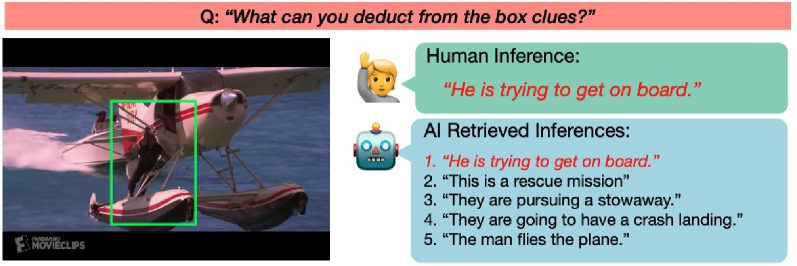
(a) Visualization 1

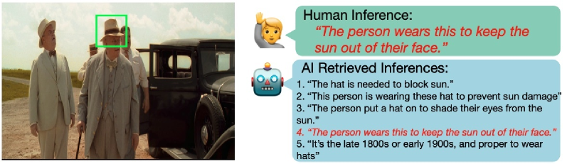
(b) Visualization 2

Figure 9: Qualitative results obtained by RPA. The machine retrieves the top-5 most likely inferences according to the box region. Red sentence indicates that the machine finds the same inference as a human expert.

VI Qualitative Results of RPA

We present two qualitative examples obtained by the RPA in Figure 9 and more examples in Figure 10. Specifically, a human expert gives a possible inference from given a regional cue specified by the box, and the machine retrieves the top-5 most likely inferences. The sentence indicates the correct match with the human’s performance. We observe from Example 1 & 2 that the machine manages to deduct human-like inference such as “He is trying to on board” from an observation of “a man under an airplane” and “prevent the sunshine” from “a wearing hat”.

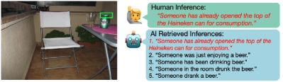
(a) Example 3

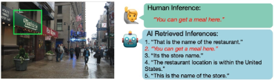
(b) Example 4

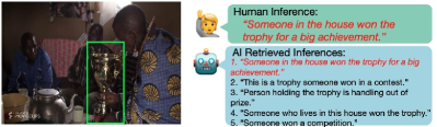
(c) Example 5

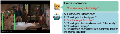
(d) Example 6

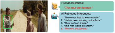
(e) Example 7

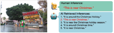
(f) Example 8

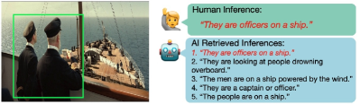
(g) Example 9

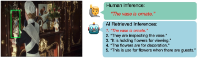
(h) Example 10

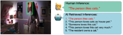
(i) Example 11

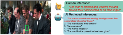
(j) Example 12

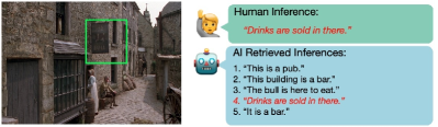
(k) Example 13

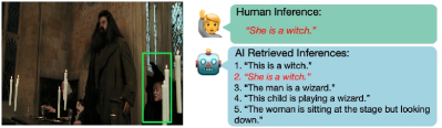
(l) Example 14

Figure 10: Qualitative results obtained by RPA. The machine retrieves the top-5 most likely inferences according to the box region. Red sentence indicates that the machine finds the same inference as a human expert.

VII Generalization of RPA on RefCOCO

We also tested the generalization of the RPA on the RefCOCO dataset using a two-stage pipeline. Specifically, we employed YoloV8 as the object detector to propose candidate object boxes. Then, we utilized the RPA to align textual sentences with the object box with the highest matching score. We evaluated the RPA using a single-prompt mode, such as “R-CTX”, “R-CPT”, to observe their respective effects.

TABLE X: Comparsion of RPA and MattNet on the RefCOCO+/g. We test with RPA ViT-L14 (336). higher=better

Model	RefCOCO ($\uparrow$)			RefCOCO+ ($\uparrow$)			RefCOCOg ($\uparrow$)
	val	testA	testB	val	testA	testB	val	test
MAttNet [72]	76.65	81.14	69.99	65.33	71.62	56.02	66.58	67.27
UNITERL [65]	81.41	87.04	74.17	75.90	81.45	66.70	74.86	75.77
MDETR [73]	86.75	89.58	81.41	79.52	84.09	70.62	81.64	80.89
RPA (R-CTX)	73.31	81.95	60.84	75.81	86.47	61.98	76.35	75.43
RPA (R-CPT)	74.04	82.80	62.81	76.40	86.34	63.12	76.59	75.47

The RPA performs better than two-stage models like MattNet on the RefCOCO+/g sets, emphasizing appearance descriptions (e.g., “a person with a yellow tie”). However, it lags behind MattNet on RefCOCO, which focuses on positional descriptions (e.g., “left person”). This discrepancy arises because MattNet explicitly encodes appearance, location, and relation information, while RPA only encodes appearance. Although RPA is adaptable to the Referring Comprehension task, it falls behind one-stage end-to-end models like MDETR. The advantage of MDETR has comes from its design to simultaneously regress box coordinates and establish visual-linguistic alignment, especially for visual grounding. In contrast, our RPA have to rely on third-party proposals from YoloV8.

VIII Conclusion

We propose a new Region-Prompted Adapter Tuning ( RPA) with a Dual-Contrastive Loss for Visual Abductive Reasoning. Specifically, our method validates that curating fine-grained regional prompts is feasible for CLIP tuning, getting back local details, and benefiting abductive reasoning. We also reveal the positive relationships between the VAR and Vanilla Visual Retrieval tasks, unifying their training processes with the Dual-Contrastive Loss. Extensive experiments show that the RPA and the new loss are robust and effective for abductive reasoning and surpass previous SOTAs. The success of the two factors also paves future ways for exploring Multi-Grained, Chain-of-Thoughts Prompts, Visual Referring Prompt, and other multiple relationships modeling on the VAR.

References

- [1] A. M. Turing, Computing machinery and intelligence. Springer, 2009.
- [2] T. Brown, B. Mann, N. Ryder, M. Subbiah, J. D. Kaplan, P. Dhariwal, A. Neelakantan, P. Shyam, G. Sastry, A. Askell et al., “Language models are few-shot learners,” Advances in neural information processing systems, vol. 33, pp. 1877–1901, 2020.
- [3] A. Radford, J. W. Kim, C. Hallacy, A. Ramesh, G. Goh, S. Agarwal, G. Sastry, A. Askell, P. Mishkin, J. Clark et al., “Learning transferable visual models from natural language supervision,” in International Conference on Machine Learning. PMLR, 2021, pp. 8748–8763.
- [4] C. Bhagavatula, R. L. Bras, C. Malaviya, K. Sakaguchi, A. Holtzman, H. Rashkin, D. Downey, S. W.-t. Yih, and Y. Choi, “Abductive commonsense reasoning,” arXiv preprint arXiv:1908.05739, 2019.
- [5] J. Hessel, J. D. Hwang, J. S. Park, R. Zellers, C. Bhagavatula, A. Rohrbach, K. Saenko, and Y. Choi, “The abduction of sherlock holmes: A dataset for visual abductive reasoning,” arXiv preprint arXiv:2202.04800, 2022.
- [6] C. Liang, W. Wang, T. Zhou, and Y. Yang, “Visual abductive reasoning,” in Proceedings of the IEEE/CVF Conference on Computer Vision and Pattern Recognition, 2022, pp. 15 565–15 575.
- [7] W. Zhao, Y. Rao, Y. Tang, J. Zhou, and J. Lu, “Videoabc: A real-world video dataset for abductive visual reasoning,” IEEE Transactions on Image Processing, vol. 31, pp. 6048–6061, 2022.
- [8] Q. Cao, B. Li, X. Liang, K. Wang, and L. Lin, “Knowledge-routed visual question reasoning: Challenges for deep representation embedding,” IEEE Transactions on Neural Networks and Learning Systems (TNNLS), vol. 33, no. 7, pp. 2758–2767, 2021.
- [9] M. Małkiński and J. Mańdziuk, “Multi-label contrastive learning for abstract visual reasoning,” IEEE Transactions on Neural Networks and Learning Systems (TNNLS), 2022.
- [10] W. Pan, Z. Zhao, W. Huang, Z. Zhang, L. Fu, Z. Pan, J. Yu, and F. Wu, “Video moment retrieval with noisy labels,” IEEE Transactions on Neural Networks and Learning Systems (TNNLS), 2022.
- [11] S.-J. Peng, Y. He, X. Liu, Y.-m. Cheung, X. Xu, and Z. Cui, “Relation-aggregated cross-graph correlation learning for fine-grained image–text retrieval,” IEEE Transactions on Neural Networks and Learning Systems (TNNLS), 2022.
- [12] S. Yan, H. Tang, L. Zhang, and J. Tang, “Image-specific information suppression and implicit local alignment for text-based person search,” IEEE Transactions on Neural Networks and Learning Systems (TNNLS), 2023.
- [13] J. Zhang, Z. Fang, H. Sun, and Z. Wang, “Adaptive semantic-enhanced transformer for image captioning,” IEEE Transactions on Neural Networks and Learning Systems (TNNLS), 2022.
- [14] B. Li, L. Y. Wu, D. Liu, H. Chen, Y. Ye, and X. Xie, “Image template matching via dense and consistent contrastive learning,” in 2023 IEEE International Conference on Multimedia and Expo (ICME). IEEE, 2023, pp. 1319–1324.
- [15] Y. Hao, C.-W. Ngo, and B. Zhu, “Learning to match anchor-target video pairs with dual attentional holographic networks,” IEEE Transactions on Image Processing, vol. 30, pp. 8130–8143, 2021.
- [16] J. Yu, H. Li, Y. Hao, B. Zhu, T. Xu, and X. He, “Cgt-gan: Clip-guided text gan for image captioning,” arXiv preprint arXiv:2308.12045, 2023.
- [17] Y. Hao, T. Mu, R. Hong, M. Wang, N. An, and J. Y. Goulermas, “Stochastic multiview hashing for large-scale near-duplicate video retrieval,” IEEE Transactions on Multimedia, vol. 19, no. 1, pp. 1–14, 2016.
- [18] B. Zhu, C.-W. Ngo, J. Chen, and Y. Hao, “R2gan: Cross-modal recipe retrieval with generative adversarial network,” in Proceedings of the IEEE/CVF Conference on Computer Vision and Pattern Recognition, 2019, pp. 11 477–11 486.
- [19] P. W. Anderson, “More is different: broken symmetry and the nature of the hierarchical structure of science.” Science, vol. 177, no. 4047, pp. 393–396, 1972.
- [20] A. Galassi, M. Lippi, and P. Torroni, “Attention in natural language processing,” IEEE Transactions on Neural Networks and Learning Systems (TNNLS), vol. 32, no. 10, pp. 4291–4308, 2020.
- [21] D. W. Otter, J. R. Medina, and J. K. Kalita, “A survey of the usages of deep learning for natural language processing,” IEEE Transactions on Neural Networks and Learning Systems (TNNLS), vol. 32, no. 2, pp. 604–624, 2020.
- [22] Y. Liu, Y. Zhang, Y. Wang, F. Hou, J. Yuan, J. Tian, Y. Zhang, Z. Shi, J. Fan, and Z. He, “A survey of visual transformers,” IEEE Transactions on Neural Networks and Learning Systems (TNNLS), 2023.
- [23] Y. Hao, S. Wang, P. Cao, X. Gao, T. Xu, J. Wu, and X. He, “Attention in attention: Modeling context correlation for efficient video classification,” IEEE Transactions on Circuits and Systems for Video Technology, vol. 32, no. 10, pp. 7120–7132, 2022.
- [24] J. Devlin, M.-W. Chang, K. Lee, and K. Toutanova, “Bert: Pre-training of deep bidirectional transformers for language understanding,” arXiv preprint arXiv:1810.04805, 2018.
- [25] C. Jia, Y. Yang, Y. Xia, Y.-T. Chen, Z. Parekh, H. Pham, Q. Le, Y.-H. Sung, Z. Li, and T. Duerig, “Scaling up visual and vision-language representation learning with noisy text supervision,” in International Conference on Machine Learning. PMLR, 2021, pp. 4904–4916.
- [26] J. Yu, Z. Wang, V. Vasudevan, L. Yeung, M. Seyedhosseini, and Y. Wu, “Coca: Contrastive captioners are image-text foundation models,” arXiv preprint arXiv:2205.01917, 2022.
- [27] L. Yuan, D. Chen, Y.-L. Chen, N. Codella, X. Dai, J. Gao, H. Hu, X. Huang, B. Li, C. Li et al., “Florence: A new foundation model for computer vision,” arXiv preprint arXiv:2111.11432, 2021.
- [28] J. Li, D. Li, C. Xiong, and S. Hoi, “Blip: Bootstrapping language-image pre-training for unified vision-language understanding and generation,” in ICML, 2022.
- [29] M. R. Cohen, “The collected papers of charles sanders peirce,” 1933.
- [30] C. Bhagavatula, R. L. Bras, C. Malaviya, K. Sakaguchi, A. Holtzman, H. Rashkin, D. Downey, W. tau Yih, and Y. Choi, “Abductive commonsense reasoning,” in International Conference on Learning Representations, 2020. [Online]. Available: https://openreview.net/forum?id=Byg1v1HKDB
- [31] R. Zellers, Y. Bisk, A. Farhadi, and Y. Choi, “From recognition to cognition: Visual commonsense reasoning,” in The IEEE Conference on Computer Vision and Pattern Recognition (CVPR), June 2019.
- [32] Y. Zhu, O. Groth, M. Bernstein, and L. Fei-Fei, “Visual7w: Grounded question answering in images,” in Proceedings of the IEEE conference on computer vision and pattern recognition, 2016, pp. 4995–5004.
- [33] M. Sabry and A. Belz, “Peft-ref: A modular reference architecture and typology for parameter-efficient finetuning techniques,” arXiv preprint arXiv:2304.12410, 2023.
- [34] B. Lester, R. Al-Rfou, and N. Constant, “The power of scale for parameter-efficient prompt tuning,” arXiv preprint arXiv:2104.08691, 2021.
- [35] Z. Zhong, D. Friedman, and D. Chen, “Factual probing is [mask]: Learning vs. learning to recall,” arXiv preprint arXiv:2104.05240, 2021.
- [36] L. Tu, C. Xiong, and Y. Zhou, “Prompt-tuning can be much better than fine-tuning on cross-lingual understanding with multilingual language models,” arXiv preprint arXiv:2210.12360, 2022.
- [37] X. Liu, K. Ji, Y. Fu, W. Tam, Z. Du, Z. Yang, and J. Tang, “P-tuning: Prompt tuning can be comparable to fine-tuning across scales and tasks,” in Proceedings of the 60th Annual Meeting of the Association for Computational Linguistics (Volume 2: Short Papers), 2022, pp. 61–68.
- [38] K. Zhou, J. Yang, C. C. Loy, and Z. Liu, “Learning to prompt for vision-language models,” International Journal of Computer Vision (IJCV), 2022.
- [39] ——, “Conditional prompt learning for vision-language models,” in Proceedings of the IEEE/CVF Conference on Computer Vision and Pattern Recognition, 2022, pp. 16 816–16 825.
- [40] C. Feng, Y. Zhong, Z. Jie, X. Chu, H. Ren, X. Wei, W. Xie, and L. Ma, “Promptdet: Towards open-vocabulary detection using uncurated images,” in Proceedings of the European Conference on Computer Vision, 2022.
- [41] Y. Du, F. Wei, Z. Zhang, M. Shi, Y. Gao, and G. Li, “Learning to prompt for open-vocabulary object detection with vision-language model,” in Proceedings of the IEEE/CVF Conference on Computer Vision and Pattern Recognition, 2022, pp. 14 084–14 093.
- [42] M. Jia, L. Tang, B.-C. Chen, C. Cardie, S. Belongie, B. Hariharan, and S.-N. Lim, “Visual prompt tuning,” in Computer Vision–ECCV 2022: 17th European Conference, Tel Aviv, Israel, October 23–27, 2022, Proceedings, Part XXXIII. Springer, 2022, pp. 709–727.
- [43] H. Bahng, A. Jahanian, S. Sankaranarayanan, and P. Isola, “Exploring visual prompts for adapting large-scale models,” arXiv preprint arXiv:2203.17274, vol. 1, no. 3, p. 4, 2022.
- [44] R. Zellers, X. Lu, J. Hessel, Y. Yu, J. S. Park, J. Cao, A. Farhadi, and Y. Choi, “Merlot: Multimodal neural script knowledge models,” in Advances in Neural Information Processing Systems 34, 2021.
- [45] Y. Yao, A. Zhang, Z. Zhang, Z. Liu, T.-S. Chua, and M. Sun, “Cpt: Colorful prompt tuning for pre-trained vision-language models,” arXiv preprint arXiv:2109.11797, 2021.
- [46] A. Shtedritski, C. Rupprecht, and A. Vedaldi, “What does clip know about a red circle? visual prompt engineering for vlms,” arXiv preprint arXiv:2304.06712, 2023.
- [47] T. Yang, Y. Zhu, Y. Xie, A. Zhang, C. Chen, and M. Li, “AIM: Adapting image models for efficient video action recognition,” in The Eleventh International Conference on Learning Representations, 2023. [Online]. Available: https://openreview.net/forum?id=CIoSZ_HKHS7
- [48] Y.-L. Sung, J. Cho, and M. Bansal, “Vl-adapter: Parameter-efficient transfer learning for vision-and-language tasks,” in Proceedings of the IEEE/CVF Conference on Computer Vision and Pattern Recognition, 2022, pp. 5227–5237.
- [49] N. Houlsby, A. Giurgiu, S. Jastrzebski, B. Morrone, Q. De Laroussilhe, A. Gesmundo, M. Attariyan, and S. Gelly, “Parameter-efficient transfer learning for nlp,” in International Conference on Machine Learning. PMLR, 2019, pp. 2790–2799.
- [50] H. Zhao, H. Tan, and H. Mei, “Tiny-attention adapter: Contexts are more important than the number of parameters,” in Conference on Empirical Methods in Natural Language Processing, 2022.
- [51] E. J. Hu, Y. Shen, P. Wallis, Z. Allen-Zhu, Y. Li, S. Wang, L. Wang, and W. Chen, “Lora: Low-rank adaptation of large language models,” arXiv preprint arXiv:2106.09685, 2021.
- [52] Y. Zhong, J. Yang, P. Zhang, C. Li, N. Codella, L. H. Li, L. Zhou, X. Dai, L. Yuan, Y. Li et al., “Regionclip: Region-based language-image pretraining,” in Proceedings of the IEEE/CVF Conference on Computer Vision and Pattern Recognition, 2022, pp. 16 793–16 803.
- [53] H. Zhang and C.-W. Ngo, “A fine granularity object-level representation for event detection and recounting,” IEEE Transactions on Multimedia, vol. 21, no. 6, pp. 1450–1463, 2018.
- [54] H. Zhang, P. Zhang, X. Hu, Y.-C. Chen, L. H. Li, X. Dai, L. Wang, L. Yuan, J.-N. Hwang, and J. Gao, “Glipv2: Unifying localization and vision-language understanding,” in Advances in Neural Information Processing Systems, 2022.
- [55] W. Wang, J. Dai, Z. Chen, Z. Huang, Z. Li, X. Zhu, X. Hu, T. Lu, L. Lu, H. Li et al., “Internimage: Exploring large-scale vision foundation models with deformable convolutions,” arXiv preprint arXiv:2211.05778, 2022.
- [56] A. Aberdam, D. Bensaïd, A. Golts, R. Ganz, O. Nuriel, R. Tichauer, S. Mazor, and R. Litman, “Clipter: Looking at the bigger picture in scene text recognition,” arXiv preprint arXiv:2301.07464, 2023.
- [57] Z. Shao, J. Han, D. Marnerides, and K. Debattista, “Region-object relation-aware dense captioning via transformer,” IEEE Transactions on Neural Networks and Learning Systems (TNNLS), 2022.
- [58] K. He, G. Gkioxari, P. Dollár, and R. Girshick, “Mask r-cnn,” in Proceedings of the IEEE international conference on computer vision, 2017, pp. 2961–2969.
- [59] Z.-Q. Zhao, P. Zheng, S.-t. Xu, and X. Wu, “Object detection with deep learning: A review,” IEEE Transactions on Neural Networks and Learning Systems (TNNLS), vol. 30, no. 11, pp. 3212–3232, 2019.
- [60] L. Jiao, R. Zhang, F. Liu, S. Yang, B. Hou, L. Li, and X. Tang, “New generation deep learning for video object detection: A survey,” IEEE Transactions on Neural Networks and Learning Systems (TNNLS), vol. 33, no. 8, pp. 3195–3215, 2021.
- [61] S.-C. Huang, Q.-V. Hoang, and T.-H. Le, “Sfa-net: A selective features absorption network for object detection in rainy weather conditions,” IEEE Transactions on Neural Networks and Learning Systems (TNNLS), 2022.
- [62] X. Bi, J. Hu, B. Xiao, W. Li, and X. Gao, “Iemask r-cnn: Information-enhanced mask r-cnn,” IEEE Transactions on Big Data, vol. 9, no. 2, pp. 688–700, 2022.
- [63] R. Girshick, J. Donahue, T. Darrell, and J. Malik, “Rich feature hierarchies for accurate object detection and semantic segmentation,” in Proceedings of the IEEE conference on computer vision and pattern recognition, 2014, pp. 580–587.
- [64] S. Ren, K. He, R. Girshick, and J. Sun, “Faster r-cnn: Towards real-time object detection with region proposal networks,” Advances in neural information processing systems, vol. 28, 2015.
- [65] Y.-C. Chen, L. Li, L. Yu, A. El Kholy, F. Ahmed, Z. Gan, Y. Cheng, and J. Liu, “Uniter: Universal image-text representation learning,” in Computer Vision–ECCV 2020: 16th European Conference, Glasgow, UK, August 23–28, 2020, Proceedings, Part XXX. Springer, 2020, pp. 104–120.
- [66] H. Tan and M. Bansal, “Lxmert: Learning cross-modality encoder representations from transformers,” in Proceedings of the 2019 Conference on Empirical Methods in Natural Language Processing, 2019.
- [67] L. Yu, P. Poirson, S. Yang, A. C. Berg, and T. L. Berg, “Modeling context in referring expressions,” in Computer Vision–ECCV 2016: 14th European Conference, Amsterdam, The Netherlands, October 11-14, 2016, Proceedings, Part II 14. Springer, 2016, pp. 69–85.
- [68] R. Krishna, Y. Zhu, O. Groth, J. Johnson, K. Hata, J. Kravitz, S. Chen, Y. Kalantidis, L.-J. Li, D. A. Shamma, M. Bernstein, and L. Fei-Fei, “Visual genome: Connecting language and vision using crowdsourced dense image annotations,” 2016. [Online]. Available: https://arxiv.org/abs/1602.07332
- [69] T.-Y. Lin, M. Maire, S. Belongie, J. Hays, P. Perona, D. Ramanan, P. Dollár, and C. L. Zitnick, “Microsoft coco: Common objects in context,” in Computer Vision–ECCV 2014: 13th European Conference, Zurich, Switzerland, September 6-12, 2014, Proceedings, Part V 13. Springer, 2014, pp. 740–755.
- [70] M. Cherti, R. Beaumont, R. Wightman, M. Wortsman, G. Ilharco, C. Gordon, C. Schuhmann, L. Schmidt, and J. Jitsev, “Reproducible scaling laws for contrastive language-image learning,” arXiv preprint arXiv:2212.07143, 2022.
- [71] T. Chen, B. Xu, C. Zhang, and C. Guestrin, “Training deep nets with sublinear memory cost,” arXiv preprint arXiv:1604.06174, 2016.
- [72] L. Yu, Z. Lin, X. Shen, J. Yang, X. Lu, M. Bansal, and T. L. Berg, “Mattnet: Modular attention network for referring expression comprehension,” in Proceedings of the IEEE conference on computer vision and pattern recognition, 2018, pp. 1307–1315.
- [73] A. Kamath, M. Singh, Y. LeCun, G. Synnaeve, I. Misra, and N. Carion, “Mdetr-modulated detection for end-to-end multi-modal understanding,” in Proceedings of the IEEE/CVF International Conference on Computer Vision, 2021, pp. 1780–1790.