CroSel: Cross Selection of Confident Pseudo Labels
for Partial-Label Learning

Abstract

Partial-label learning (PLL) is an important weakly supervised learning problem, which allows each training example to have a candidate label set instead of a single ground-truth label. Identification-based methods have been widely explored to tackle label ambiguity issues in PLL, which regard the true label as a latent variable to be identified. However, identifying the true labels accurately and completely remains challenging, causing noise in pseudo labels during model training. In this paper, we propose a new method called CroSel, which leverages historical prediction information from models to identify true labels for most training examples. First, we introduce a cross selection strategy, which enables two deep models to select true labels of partially labeled data for each other. Besides, we propose a novel consistent regularization term called co-mix to avoid sample waste and tiny noise caused by false selection. In this way, CroSel can pick out the true labels of most examples with high precision. Extensive experiments demonstrate the superiority of CroSel, which consistently outperforms previous state-of-the-art methods on benchmark datasets. Additionally, our method achieves over 90% accuracy and quantity for selecting true labels on CIFAR-type datasets under various settings.

1 Introduction

The past few years have seen an increased interest in deep learning due to its outstanding performance in various application domains, including image processing [3], automatic driving [27], and medical diagnosis [18]. The success of deep learning heavily relies on a massive amount of fully labeled data. However, it is challenging to obtain a large-scale dataset with completely accurate annotations in the real world. To address this challenge, many researchers have explored a promising weakly supervised learning problem called partial-label learning (PLL) [4, 5, 22, 25, 26], which allows each training example to have a set of candidate labels that includes the true label. This problem arises in many real-world tasks such as automatic image annotation [2] and facial age estimation [17].

As PLL focuses on multi-class classification, there is only one ground-truth label for each training example, and other labels in the candidate label set are actually wrong (false positive) labels, which would have a negative impact on model training. Therefore, there exists the challenge of label ambiguity in PLL. To address this challenge, the current mainstream solution is to disambiguate the candidate labels so as to figure out the true label for each training instance [10, 28, 13, 5, 14]. However, most of the existing disambiguation methods normally leverage simple heuristics to iteratively update the labeling confidences or pseudo labels [5, 14, 22, 26], which could not achieve convincing performance in identifying the true label during the training phase. Generally, if more true labels of training instances can be identified, we can train a better model. This motivates us to focus on identifying the true labels of training instances as many as possible, thereby training a desired model.

In this paper, we propose a method called CroSel (Cross Selection of Confident Pseudo Labels), which leverages historical prediction information from deep neural networks to accurately identify true labels for most training examples. Our selecting criteria are based on the assumption that if a model consistently predicts the same label for an input image with high confidence and low volatility, then that label has a high probability of being the true label for that example. Using the cross selection strategy, the true labels of the vast majority of training examples can be accurately identified, with only negligible noise. Moreover, in order to avoid sample waste and tiny noise resulting from the selection, we also proposed a co-mix consistency regularization to generate trainable targets for all examples. This regulation term serves as an essential complement to our method, which can further enhance the scope and accuracy of our selection of “true” labels. The algorithm details are shown in Section 3.

Our main contributions are summarized as follows:

• We propose a cross selection strategy to select the confident pseudo labels in the candidate label set based on historical prediction information. This strategy shows high selection precision and selection ratio of “true” labels in the experiment.

• We propose a new consistency loss regularization term that can leverage MixUp [30] to enhance the data and generate trainable targets as an important supplement to our method.

• We experimentally show that CroSel achieves state-of-the-art performance on common benchmark datasets. We also provide extensive ablation studies to examine the effect of the different components of CroSel.

2 Related Work

Figure 1: The left side of the figure is a brief example of our memory bank that stores the softmax output of the model for the last $t$ epochs, which is updated by the FIFO (First In First Out) principle; the middle is the cross selection strategy: within each epoch, data subsets $\mathcal{D}_{\mathrm{sel}}$ with confident pseudo-labels are selected from the MB of each network, which produce loss function $\mathcal{L}_{\mathrm{l}}$ to the training process for the other network; the right side illustrates our co-mix regularization term and the corresponding loss function $\mathcal{L}_{\mathrm{cr}}$ .

Partia-Label Learning.  This setting allows each training example to be annotated with a set of candidate labels for which the ground truth label is guaranteed to be included. However, label ambiguity can pose a significant challenge in PLL. Early methods used an averaging strategy, which tends to treat each candidate label equally. [4, 31] But such methods are easily affected by negative labels in the candidate label set, thus forming wrong classification boundaries. Afterwards, the identification-based method [10, 28, 13] has received more attention from the community, which regard the ground-truth label as a latent variable, and will maintain a confidence level for each candidate label. For instance, Yu et al. [28] introduce the maximum margin constraint to PLL problems, trying to optimize the margin between the model outputs from candidate labels and other negative labels. This method has shown better performance in disambiguating labels.

Recently, partial-label learning has been combined with deep networks, leading to significant improvements in performance. Feng et al. [5] assume that partial labels come from a uniform generation model and give a mathematical formulation, which is adopted by most of the algorithms proposed later. Based on this, they also propose an algorithm for classification consistency and risk consistency. PRODEN [14] assumes the true label should be the one with the smallest loss among the candidate labels, and improve the classification risk algorithm accordingly. Wen et al. [25] propose a risk-consistent leveraged weighted loss with label-specific candidate label sampling. PiCO [22] innovatively introduced contrastive learning [16] to the field and provided a solid theoretical analysis based on EM. CRDPLL [26] proposed a new consistency loss item in this field and treat the parts that are not selected as candidate labels as supervision information. SoLar [21] focuses on solutions to PLL problems in more realistic scenarios such as class-imbalanced settings.

Sample selection.  Sample selection is a popular technique in deep learning, especially for datasets with noisy labels or incomplete annotations. Then an obvious idea is to separate the clean samples and noisy samples in the mixed dataset. To address this issue, many existing works adopt the small loss criterion [8, 9], which assumes that clean samples tend to have a smaller loss than noisy samples during training. MentorNet [9] is a representative work that let the teacher model pick up clean samples for the student model. Co-teaching [8] constructs a double branches network to select clean samples for each branch, which is different from the teacher-student approach since none of the models supervise the other but rather help each other out. This idea was improved by some research later [29, 23] to achieve better performance. Curriculum learning is also applied to this field [7], which considers clean labeled data as an easy task, while noisily labeled data as a harder task. Guo et al. [6] split data into subgroups according to their complexities, in order to optimize the training objectives in the early stage of course learning. OpenMatch [20] trains $n$ OVA classifiers to select the in-distribution samples under the open set setting. Generative models such as Beta Mixture Model  [1] and Gaussian Mixture Model [12] are also used to fit loss functions to distinguish clean labels from noisy labels. Recently, the fluctuation magnitude of the output of the same example is also considered as an important credential to judge whether the label is clean [24].

3 Our methods

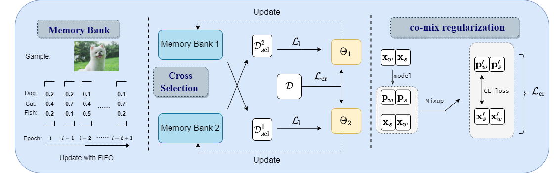
In this section, we provide a detailed explanation of how our algorithm works. Our method is composed of two main components: a cross selection strategy that utilizes two models to select confident pseudo labels for each other, and a consistency regularization term that is applied across different data augmentation versions. The latter part not only addresses the issue of label waste resulting from the selection process but also enhances the quantity and accuracy of selections. The pseudo-code for our algorithm is presented in Algorithm 1.

3.1 Problem setting

Suppose the feature space is $\mathcal{X}\in\mathbb{R}^{d}$ with $d$ dimensions and the label space is $\mathcal{Y}=\{1,2,\dots,k\}$ with $k$ classes. We are given a dataset $\mathcal{D}=\{(\boldsymbol{x}_{i},S_{i})\}_{i=1}^{n}$ with n examples, where the instance $\boldsymbol{x}_{i}\in\mathcal{X}$ and the candidate label set $S_{i}\subset\mathcal{Y}$. Same as previous studies, we assume that the true label $y_{i}\in\mathcal{Y}$ of each input $\boldsymbol{x}_{i}$ is concealed in $S_{i}$.

Our aim is to train a multi-class classifier $f:\mathbb{R}^{d}\rightarrow\mathbb{Y}$ that minimizes the classification risk on the given dataset. For our classifier $f$, we use $f(\boldsymbol{x})$ to represent the output of classifier $f$ on given input $\boldsymbol{x}$. And we use $\hat{y}=\mathrm{argmax}_{y\in\mathcal{Y}}f_{y}(\boldsymbol{x})$ to denote the prediction of our classifier, where $f_{y}(\boldsymbol{x})$ is the $y\text{-}$th coordinate of $f(\boldsymbol{x})$.

Algorithm 1 Pseudo-code of CroSel

  Input: Training dataset $\mathcal{D}=\{(\boldsymbol{x}_{i},S_{i})\}_{i=1}^{n}$, consistency regularization parameter $\lambda_{\mathrm{cr}}$, sharpen parameter $T$, confidence threshold $\gamma$, memory bank $\mathrm{MB}^{(1)}$, $\mathrm{MB}^{(2)}$, network $\Theta^{(1)},\Theta^{(2)}$, epoch $E$, iteration $I$.

  Procedure:

  $\mathrm{MB}^{(1)},\mathrm{MB}^{(2)},\Theta^{(1)},\Theta^{(2)}=\mathrm{WarmUp}(\mathrm{MB}^{(1)},\mathrm{MB}^{(2)},\Theta^{(1)},\Theta^{(2)},\mathcal{D})$.   //  CC algorithm

  for $e=1$ to $E$ do

     Select labeled dataset $\mathcal{D}_{\mathrm{sel}}^{1}$ through $\mathrm{MB}^{(1)}$.

     Select labeled dataset $\mathcal{D}_{\mathrm{sel}}^{2}$ through $\mathrm{MB}^{(2)}$.  //  Eq. (4)

     for $k=1,2$  do

        for $i=1$ to $I$ do

           Fetch a labeled batch $\hat{B}_{i}$ from the opposite selected dataset $\mathcal{D}_{\mathrm{sel}}^{\thicksim k}$.

           Fetch a batch $B_{i}$ from the training dataset $\mathcal{D}$.

           Compute the loss $L$ among the two batches $\hat{B}_{i}$ and $B_{i}$ through Eq. (13).

           Update the weight of $\Theta^{k}$ by optimizer.

        end for

        Update the memory bank $\mathrm{MB}^{(k)}$ through the FIFO principle.

     end for

  end for

3.2 Selection Strategy

In the current partial-label learning task, the large number of candidate labels can confuse classifier, making it difficult for the classifier to capture specific features belonging to a certain label. Therefore, our goal is to identify the most likely true label among the candidate labels and eliminate the interference of other negative labels during model training. By selecting these “true” labels, we can train the data with a supervised learning approach.

Warm up. Before selecting, we warm up the network using the entire training set. The goal of this stage is to reduce the classification risk of the input $x$ to the whole set of candidate labels $S$, and obtain some historical information that can be used to select. Therefore, here we use CC algorithm [5] to warm up models for 10 epochs. At the same time, we’ll update the value of memory bank $\mathrm{MB}$.

Selecting criteria. We have three criteria for selecting the confident pseudo labels from the candidate label set. Depending on the setup of our problem, the true label of each example must be in its candidate label set. This is our first criterion. In addition, we believe that an example’s predicted label is likely to be the true label if the model predicts it with high confidence and low fluctuation. To determine the latter, we maintain a memory bank $\mathrm{MB}$ to store the historical prediction information of this neural network.

The size of the memory bank is $t\times n\times k$, where $t$ denotes the length of time it stores, $n$ is the length of dataset, and $k$ is the number of categories in the classification. In other words, $\mathrm{MB}$ stores the output after softmax of the model in the last $t$ epochs. $\mathrm{MB}$ is structured as a queue, with each element being a $k$-dimensional vector $\boldsymbol{q}$ representing the output of an example in a particular epoch. We update $\mathrm{MB}$ with the FIFO principle. These selection criteria can be summarized as follows.

$$\beta_{1} =(\mathrm{argmax}(\boldsymbol{q}^{i})\in S),$$ (1)

$$\beta_{2} =(\mathrm{argmax}(\boldsymbol{q}^{i})==\mathrm{argmax}(\boldsymbol{q}^{i+1})),$$ (2)

$$\beta_{3} =(\frac{1}{t}\sum_{i=1}^{t}\mathrm{max}(\boldsymbol{q}^{i})>\gamma).$$ (3)

where $i=1,2...t$, $t\geq 2$, $\gamma$ is the confidence threshold of selection. $\beta_{1}$ lets our selected label be in the candidate label set. $\beta_{2}$ limits that the label we picked has not flipped in the past $t$ epochs, which is a volatility consideration and $\beta_{3}$ ensures that the label we selected has a high confidence level. The final selected dataset is $\mathcal{D}_{\mathrm{sel}}$:

$$\mathcal{D}_{\mathrm{sel}}={((\boldsymbol{x}_{i},\mathrm{argmax}(\boldsymbol{q}^{t}_{i}))|(\beta_{1}^{i}\wedge\beta_{2}^{i}\wedge\beta_{3}^{i})=1,\boldsymbol{x}_{i}\in\mathcal{D})}$$ (4)

Selected label loss.  After selecting the high-confidence examples, we obtain a dynamically updated data subset $\mathcal{D}_{\mathrm{sel}}=(X,\hat{Y})$. Each tuple of the subset has an instance $\boldsymbol{x}$ and a selected label $\hat{y}=\mathrm{argmax}(\boldsymbol{q}^{t})$. In this configuration, we can use the basic cross-entropy loss to deal with this part of samples.

$$\mathcal{L}_{\mathrm{l}}=\frac{1}{|\mathcal{D}_{\mathrm{sel}}|}{\sum_{\boldsymbol{x}\in\mathcal{D}_{\mathrm{sel}}}}\mathrm{CE}(f(\boldsymbol{x}_{\mathrm{w}}),\hat{y})$$ (5)

where $\mathrm{CE}(\cdot,\cdot)$ denotes the cross entropy loss, $\boldsymbol{x}_{\mathrm{w}}$ denotes the weak augmented version of example $\boldsymbol{x}$.

Cross Selection.  However, In the process of selecting labels, it is difficult to guarantee that the selected labels are 100% accurate. In order to maximize the accuracy of selection, we propose a cross selection framework based on the idea of ensemble learning. Specifically, we train two identical models $\Theta^{(1)}$ and $\Theta^{(2)}$ through the same training and label selection process. By forming different decision boundaries, the two models can adaptively correct most of the errors even if there is noise in the selected confident pseudo labels.

To maximize the accuracy of the selected labels, we employ a cross-supervised training process. This involves using the selected dataset $\mathcal{D}_{\mathrm{sel}}^{1}$ from $\mathrm{MB}^{(1)}$ to train $\Theta^{(2)}$, and vice versa, using the selected dataset $\mathcal{D}_{\mathrm{sel}}^{2}$ from $\mathrm{MB}^{(2)}$ to train $\Theta^{(1)}$. By doing so, the two models can learn from each other and further improve their ability to select true labels. In the test process, we will average the output of the two models to reduce the variance.

$$f^{\prime}(\boldsymbol{x})=\frac{1}{2}(f^{1}(\boldsymbol{x})+f^{2}(\boldsymbol{x}))$$ (6)

where $f^{\prime}(\boldsymbol{x})$ denotes the final output of our method in the test process, $f^{1}(\boldsymbol{x})$ denotes the output of $\Theta^{(1)}$, $f^{2}(\boldsymbol{x})$ denotes the output of $\Theta^{(2)}$.

3.3 Co-mix Consistency Regulation

Motivation.  When dealing with complex partial-label learning tasks, our label selection strategy may not accurately select the true labels for all examples. If we only use the selected examples with their corresponding labels, it will result in a significant amount of wasted data, which contradicts our goal of utilizing as many examples as possible. Therefore, we aim to provide a trainable target for the remaining examples that are not selected. However, our setting differs from traditional semi-supervised learning as the proportion of unlabeled examples is relatively small. So it is unreasonable to directly transfer the existing semi-supervised learning tools to unlabeled data like other weakly supervised learning methods.

Motivated by this, we hope to propose a regularization term that can serve as an important supplement to our method and help us select examples. We proposed the co-mix regularization term, which employs two widely used data augmentation methods: weak augmentation and strong augmentation, to generate pseudo-labels as training targets for consistency regularization. We further employ MixUp to further enhance the data. It is worth mentioning that the term ”pseudo labels” in this part specifically refers to the soft labels generated from different data augmentation versions, rather than the confident hard labels selected during the selection process.

Pseudo label generating. Consistency loss is a simple but effective idea in weakly supervised learning, whose key point is to reduce the gap between the output of two perturbed examples after passing through the model. As discussed in the previous section, we used two widely used data augmentations: ’weak’ and ’strong’, and crossed them to generate pseudo labels. Specifically, as stated in Figure 1, the pseudo label corresponding to weak augmented example is generated by strong augmented example, while the pseudo label corresponding to strong augmented example is generated by weak augmented example.

To generate these pseudo labels, we fix the parameters of the neural network, and pass the augmented images through the model to get the logits output. And we perform two operations on the logits, sharpening and normalization. For sharpening operation, we use a hyper parameter $T$, the more $T$ goes to zero, the more logits tend to become a one-hot distribution. These two operations can be summarized by the following formula.

$$\boldsymbol{p}_{i}=\begin{cases}\frac{\exp(f_{j}(\boldsymbol{x})^{\frac{1}{T}})}{{\textstyle\sum_{j\in S}\exp(f_{j}(\boldsymbol{x})^{\frac{1}{T}})}}&\text{$i\in S$}\\ 0&\text{$i\notin S$}\end{cases}$$ (7)

where $\boldsymbol{p}_{i}$ denotes the $i\text{-}_{th}$ coordinate of pseudo label.

MixUp.  After generating the pseudo labels of each example, we end up with two datasets that can be trained: $(X_{\mathrm{w}},P_{\mathrm{s}})$ and $(X_{\mathrm{s}},P_{\mathrm{w}})$. The subscripts w and s indicate the type of data augmentation used, i.e., weak or strong. Then, We spliced the two datasets together to further enhance the data with MixUp. [30] For a pair of two examples with their corresponding pseudo labels $(\boldsymbol{x}_{1},\boldsymbol{p}_{1}),(\boldsymbol{x}_{2},\boldsymbol{p}_{2})$, we compute $(\boldsymbol{x}^{\prime},\boldsymbol{p}^{\prime})$ by the following formula:

$$\lambda\sim{\mathrm{Beta}(\alpha,\alpha)}$$ (8)

$$\lambda^{\prime}=\mathrm{max}(\lambda,1-\lambda)$$ (9)

$$\boldsymbol{x}^{\prime}=\lambda^{\prime}\boldsymbol{x}_{1}+(1-\lambda^{\prime})\boldsymbol{x}_{2}$$ (10)

$$\boldsymbol{p}^{\prime}=\lambda^{\prime}\boldsymbol{p}_{1}+(1-\lambda^{\prime})\boldsymbol{p}_{2}$$ (11)

Then we can use the typical cross-entropy loss on every example, the consistency regulation loss will be:

$$\mathcal{L}_{\mathrm{cr}}=\frac{1}{2n}{\sum_{i=1}^{2n}}\mathrm{CE}(f(\boldsymbol{x}^{\prime}),{\boldsymbol{p}^{\prime}})$$ (12)

where $\mathrm{CE}(\cdot,\cdot)$ denotes the softmax cross entropy loss, $n$ denotes the length of a dataset.

Table 1: Accuracy(mean ± std) comparisons on benchmark datasets.

Dataset	$q$	Ours	CRDPLL	PiCO	PRODEN	LWS	CC
CIFAR-10	$q=0.1$	97.31 ± 0.04%	97.41 ± 0.06%	96.10 ± 0.06%	95.66 ± 0.08%	91.20 ± 0.07%	90.73 ± 0.10%
	$q=0.3$	97.50 ± 0.05%	97.38 ± 0.04%	95.74 ± 0.10%	95.21 ± 0.07%	89.20 ± 0.09%	88.04 ± 0.06%
	$q=0.5$	97.34 ± 0.05%	96.76 ± 0.05%	95.32 ± 0.12%	94.55 ± 0.13%	80.23 ± 0.21%	81.01 ± 0.38%
SVHN	$q=0.1$	97.71 ± 0.05%	97.63 ± 0.06%	96.58 ± 0.04%	96.20 ± 0.07%	96.42 ± 0.09%	96.99 ± 0.17%
	$q=0.3$	97.96 ± 0.05%	97.65 ± 0.07%	96.32 ± 0.09%	96.11 ± 0.05%	96.15 ± 0.08%	96.67 ± 0.20%
	$q=0.5$	97.86 ± 0.06%	97.70 ± 0.05%	95.78 ± 0.05%	95.97 ± 0.03%	95.79 ± 0.05%	95.83 ± 0.23%
CIFAR-100	$q=0.01$	84.24 ± 0.09%	82.95 ± 0.10%	74.89 ± 0.11%	72.24 ± 0.12%	62.03 ± 0.21%	66.91 ± 0.24%
	$q=0.05$	83.92 ± 0.24%	82.38 ± 0.09%	73.26 ± 0.09%	70.03 ± 0.18%	57.10 ± 0.17%	64.51 ± 0.37%
	$q=0.10$	84.07 ± 0.16%	82.15 ± 0.20%	70.03 ± 0.10%	69.82 ± 0.11%	52.60 ± 0.54%	61.50 ± 0.36%

3.4 Algorithm overview

Overall loss.  In the formal training phase, our loss function will be composed of two parts, the supervised loss $\mathcal{L}_{l}$ in the selected label set $\mathcal{D}_{\mathrm{sel}}$ and the consistency regularization item loss $\mathcal{L}_{\mathrm{cr}}$. The two will be dynamically combined into the final loss function by a hyperparameter.

$$\mathcal{L}_{\mathrm{all}}=\mathcal{L}_{\mathrm{l}}+\mathcal{L}_{\mathrm{cr}}*\lambda_{\mathrm{d}}$$ (13)

$\lambda_{\mathrm{d}}$ is a dynamically changing parameter, $\mathcal{L}_{l}$ and $\mathcal{L}_{\mathrm{cr}}$ can be calculated by Eq. (5) and Eq. (12), respectively. The use of MixUp can cause significant changes to the original feature space, making it necessary to adjust the weight of the regularization term in the loss function as the number of selected samples increases. To achieve this, we proposed a gradually decreasing $\lambda_{\mathrm{d}}$ with the increase of selected samples. We can control the magnitude of $\lambda_{\mathrm{d}}$ with a set hyperparameter $\lambda_{\mathrm{cr}}$. The updated rules of $\lambda_{\mathrm{d}}$ are as follows.

$$\lambda_{\mathrm{d}}=(1-r_{\mathrm{s}})*\lambda_{\mathrm{cr}}$$ (14)

where $r_{\mathrm{s}}$ denotes the percentage of labeled data that we picked out, $\lambda_{\mathrm{cr}}$ is a hyperparameter that collaboratively adjusts the ratio of two loss items.

4 Experiments

In this section, we provide a detailed description of the experiments we conducted. We introduce the experimental setup and present our main experimental results. Additionally, we present the findings of our ablation experiments.

4.1 Experimental Setup

Datasets. We used three widely used benchmarks in this field: SVHN [15], CIFAR-10 [11] and CIFAR-100 [11]. The way we generate partial labels is by flipping the negative labels $\overline{y}\neq y$ of the example with a set probability $q=P(\overline{y}\in S|\overline{y}\neq y)$. With the increase of $q$, the noise of the dataset increases gradually. Following PiCO [22], we consider $q=\{0.01,0.05,0.1\}$ for CIFAR-100 and $q=\{0.1,0.3,0.5\}$ for other datasets.

Compared methods.  We choose five well-performed partial-label learning algorithms to compare:

• CRDPLL [26], an algorithm that takes non-candidate labels as supervision information and proposes a new consistency loss term between augmented images.

• PiCO [22], a theoretical solid framework that combines contrastive learning and prototype-based label disambiguation algorithm.

• LWS [25], an algorithm that wants to balance the risk error between the candidate label set and the non-candidate label set.

• PRODEN [14], a self-training algorithm that dynamically updates the confidence of candidate labels.

• CC [5], an algorithm that wants to minimize the classification error of the whole candidate label sets.

Table 2: Selected ratio and selected accuracy(mean ± std) on benchmark datasets. S-ratio represents the selected ratio and S-acc represents selected accuracy in $\mathcal{D}_{\mathrm{sel}}$.

Datasets	Setting	Index	Performance
CIFAR-10	$q=0.1$	S-ratio	99.09 ± 0.07%
		S-acc	99.79 ± 0.05%
	$q=0.3$	S-ratio	98.10 ± 0.10%
		S-acc	99.55 ± 0.03%
	$q=0.5$	S-ratio	96.25 ± 0.12%
		S-acc	99.44 ± 0.06%
SVHN	$q=0.1$	S-ratio	97.25 ± 0.14%
		S-acc	99.84 ± 0.06%
	$q=0.3$	S-ratio	76.42 ± 0.21%
		S-acc	99.77 ± 0.06%
	$q=0.5$	S-ratio	73.21 ± 0.15%
		S-acc	99.34 ± 0.02%
CIFAR-100	$q=0.01$	S-ratio	96.58 ± 0.13%
		S-acc	99.71 ± 0.06%
	$q=0.05$	S-ratio	95.45 ± 0.21%
		S-acc	98.29 ± 0.15%
	$q=0.10$	S-ratio	93.61 ± 0.12%
		S-acc	97.93 ± 0.11%

Implementations.  Our implementation is based on PyTorch [19]. We use WRN-34-10 (short for Wide-ResNet-34-10) as the backbone model with a weight decay of 0.0001 on all the datasets for all methods. We set the batch size as 64 and total epochs as 200, using SGD as optimizer with a momentum of 0.9, and set the initial learning rate as 0.1, which is divided by 10 after 100 and 150 epochs respectively. For the hyper parameter in our method, We set $t=3$, $\alpha=0.75$, $T=0.5$ for all datasets, and $\lambda_{\mathrm{cr}}=1$ for CIFAR-100, $\lambda_{\mathrm{cr}}=4$ for others. For the selection threshold, we set $\gamma=0.9$ for CIFAR-type datasets, and $\gamma=0.85$ for SVHN. We present the mean and standard deviation in each case based on three independent runs with different random seeds.

Table 3: Results for the study of scope of co-mix regularization.

Setting	Scope	Index	Performance
CIFAR-10 $q=0.5$	All data	acc	97.34%
		S-ratio	96.25%
		S-acc	99.44%
	Unseleted data	acc	90.32%
		S-ratio	93.27%
		S-acc	95.72%
	None	acc	81.01%
		S-ratio	90.23%
		S-acc	89.72%
CIFAR-100 $q=0.1$	All data	acc	84.07%
		S-ratio	93.61%
		S-acc	97.93%
	Unseleted data	acc	77.61%
		S-ratio	90.12%
		S-acc	97.63%
	None	acc	70.68%
		S-ratio	78.65%
		S-acc	96.22%

4.2 Main empirical results

As shown in Table 1, our methods achieve state-of-the-art results on all the settings except CIFAR-10 with $q=0.1$. Notably, on the complex dataset CIFAR-100, our method significantly improves performance.

However, a counter-intuitive phenomenon appears in our experiment, that is, the performance of our method does not necessarily decline strictly with the increase of noise $q$; on the contrary, it may perform best in the case of moderate noise. We believe the possible reason for this phenomenon is that: On the one hand, when generating pseudo labels, we normalize them according to Eq. (7). That is to say, as the number of candidate labels increases, the ingredients involved in MixUp will also increase, leading to better-enhanced data interpolation. On the other hand, the increase of candidate labels also represents the increase of noise, which can have a negative impact on the algorithm’s performance. Therefore, CroSel performs well in cases of intermediate noise, representing an optimal solution found in such a trade-off problem.

Table 2 presents the selection ratio and accuracy of CroSel in selecting the true labels for the selected label dataset $\mathcal{D}_{\mathrm{sel}}$. It is evident that, CroSel can accurately select the true labels of most examples in the dataset under various noise conditions. Notably, for CIFAR-10 and CIFAR-100, the selection ratio and accuracy are over $90\%$ both. However, in SVHN, the selection ratio drops significantly with the increase of noise. This could be attributed to the fact that digital images in SVHN have relatively simple shape features, and MixUp may significantly disturb the feature space.

(a) CTAFR-10 Accuracy

(b) CTAFR-10 Selected Ratio

(c) CTAFR-10 Selected Accuracy

(d) CTAFR-100 Accuracy

(e) CTAFR-100 Selected Ratio

(f) CTAFR-100 Selected Accuracy

Figure 2: Parameter test for $\lambda_{\mathrm{cr}}$ on CTAFR-10 and CTAFR-100.

4.3 Ablation study

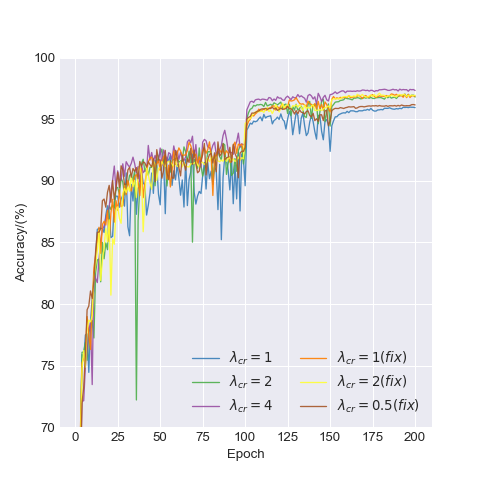
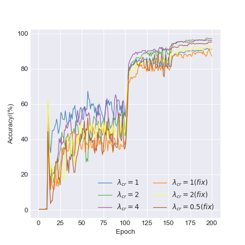
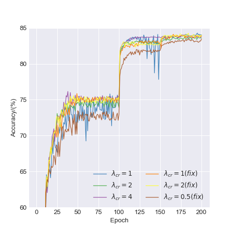
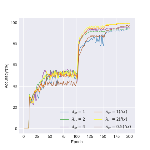
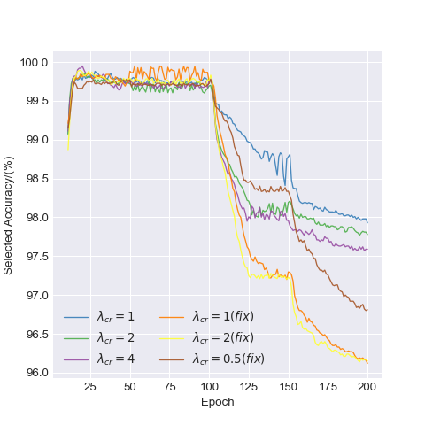
Parameter test on $\lambda_{\mathrm{cr}}$. In this experiment, we test the parameter $\lambda_{\mathrm{d}}$, which weights the contribution of the consistency regularization term to the training loss. As mentioned in Eq. (14), the parameter $\lambda_{\mathrm{d}}$ is directly influenced by the hyperparameter $\lambda_{\mathrm{cr}}$. Therefore, We test $\lambda_{\mathrm{cr}}=\{1,2,4\}$ on CIFAR-10 ($q=0.5$) and CIFAR-100 ($q=0.1$). At the same time, we also try to fix the parameter $\lambda_{\mathrm{d}}$, that is, its value is not related to the selection ratio $r_{\mathrm{s}}$. This setting we denote by $\lambda_{\mathrm{cr}}(fix)$, we test $\lambda_{\mathrm{cr}}(fix)=\{0.5,1,2\}$. The results are visualized in Figure 2, and detailed data can be found in Appendix B.3.

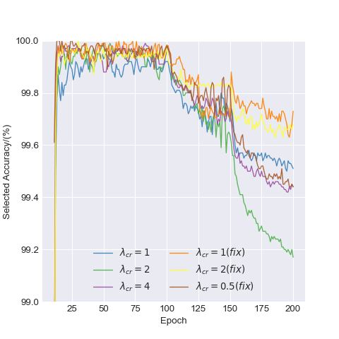
As mentioned in Table 2 above, CroSel achieves a very high selection ratio. When using a dynamically changing $\lambda_{\mathrm{d}}$, the contribution made by the regularization term would be quite small in the later stages as the learning rate decays. In contrast, with a fixed value of $\lambda_{\mathrm{d}}$, the regularization term would still have a significant contribution in the later stages. Although the accuracy rate on the test set does not show a significant difference between different parameters, the selection effect is critical. A too large contribution of the regularization item will slightly improve the selection ratio at the cost of a decrease in the selection accuracy, which goes against the original intention of our algorithm design. Therefore, we finally decided to use dynamically changing parameters. In other words, we want the algorithm to return to a supervised learning setting with minimal noise as much as possible at the end of the training process.

The influence on the scope of consistency regulation term. The preceding ablation experiment explored the magnitude of the co-mix regularization, while this experiment focused on the scope of the regularization term. As described in Section 3, our co-mix regularization is designed to avoid sample waste. As such, a natural idea is to apply the regularization term to the unselected samples, as in traditional semi-supervised learning. However, our setting differs from traditional semi-supervised learning in that our unselected data only constitutes a small portion of all the data. So we conducted experiments by trying three cases: no regularization term, using the regularization term only for the unselected dataset, and using the regularization term for all examples.

The results in Table 3 suggest that with the expansion of the application scope of co-mix regularization term, the model’s performance steadily improves, and the number of selected labeled examples also gradually increases. This also shows that our co-mix regularization term and selection strategy can achieve a mutually beneficial effect.

Table 4: Accuracy(mean ± std) on ablation study on select criteria.

Setting	$t$	Accuracy	$\gamma$	Accuracy
CIFAR-10 $q=0.3$	$t=2$	97.03%	$\gamma=0.8$	96.24%
	$t=3$	97.50%	$\gamma=0.9$	97.50%
	$t=4$	96.15%	$\gamma=0.95$	97.38%
CIFAR-100 $q=0.1$	$t=2$	82.74%	$\gamma=0.8$	80.20%
	$t=3$	84.07%	$\gamma=0.9$	84.07%
	$t=4$	83.56%	$\gamma=0.95$	83.56%

Whether the selection criteria are strict or lenient.  The two parameters $t$ and $\gamma$ in Eq. (2) and Eq. (3) determine the strictness of our selection criteria. $t$ represents the length of historical information stored in $\mathrm{MB}$, while $\gamma$ represents the select threshold for the average prediction confidence of the model for the example prediction in the past $t$ epochs. A larger $t$ and a higher $\gamma$ represent a stricter selection criterion, resulting in a smaller $\mathcal{D}_{\mathrm{sel}}$ size but higher precision, which can affect model training. During the early stages, it may be difficult to select enough examples under the condition of using stricter selection criteria. Therefore, in this and the next ablation experiment, we set the label flipping probability $q$ to 0.3 on CIFAR-10. However, in the later stages, the impact of selection criteria on the final accuracy rate is not significant if the initial stage is passed smoothly. Our experiment shows that $t=3$ and $\gamma=0.9$ are suitable values that can be applied to most experimental environments. The experimental results are presented in Table 4 and Appendix B.3.

Table 5: Results for Augmentations test on $\mathcal{D}_{\mathrm{sel}}$.

Setting	Aug type	Accuracy	Selected ratio
CIFAR-10 $q=0.3$	None	96.91%	97.44%
	Weak	97.50%	98.10%
	Strong	97.22%	96.26%
CIFAR-100 $q=0.1$	None	83.74%	90.48%
	Weak	84.07%	93.61%
	Strong	81.01%	79.16%

The influence on data augmentation on $\mathcal{D}_{\mathrm{sel}}$. Data augmentations play a crucial role in weakly supervised learning. However, our selection criteria rely on historical prediction information to select examples with high confidence, and we cannot guarantee that stronger data augmentations will necessarily lead to better results and selection effects. So, in this part, we explore the impact of data augmentation on $\mathcal{D}_{\mathrm{sel}}$ and its influence on label selection and overall training. As shown in Table 5, weak augmentation is a more appropriate and effective choice. However, because of the impact of regular items, even if data augmentation is not used on $\mathcal{D}_{\mathrm{sel}}$, there is no significant performance degradation. Strong data augmentation has an adverse effect on the selection of examples, especially in CIFAR-100, which may also be related to the fact that the historical predictions stored in $\mathrm{MB}$ are produced by data that have not been augmented.

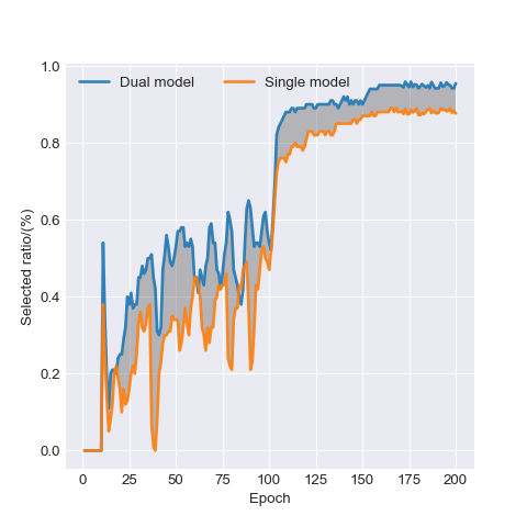
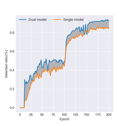
The influence on double model. As recognized by the community, dual models tend to achieve better performance than single models. We are curious about how effective our selection criteria would be without the adaptive error correction capability of cross selection. Figure 3 visualizes the gap in the selection ratio between dual-model and single-model training. It shows that our cross selection strategy can select samples more comprehensively, and on average, about 10% more training examples can be selected on each dataset. However, the effectiveness of our algorithm is not solely due to the dual model. Even when using a single model with our selection criteria, the accuracy rate on the test set only decreases by 0.83% and 2.68% on CIFAR-10 and CIFAR-100 respectively. Furthermore, the high precision of selection is reflected in both settings. Detailed results can be found in Table 6 and Appendix.B.3.

(a) CTAFR-10 comparison

(b) CTAFR-100 comparison

Figure 3: Selection ratio comparison between dual model and single model on CTAFR-10 and CTAFR-100.

Table 6: Comparison between Dual model and Single model.
S-acc represents selected accuracy in $\mathcal{D}_{\mathrm{sel}}$.

Setting	Model	Accuracy	S-acc
CIFAR-10 $q=0.5$	Single model	96.51%	99.72%
	Dual model	97.34%	99.44%
CIFAR-100 $q=0.1$	Single model	81.39%	98.35%
	Dual model	84.07%	97.93%

5 Conclusion

This work introduces CroSel, a novel partial-label learning method that leverages historical prediction information to select the confident pseudo labels from candidate label sets. The proposed method consists of two parts: a cross selection strategy that enables two deep models to select “true” labels for each other, and a consistent regularization term co-mix that avoids sample waste and tiny noise caused by false selection. Empirically, extensive experiments demonstrate the superiority of CroSel, which consistently outperforms previous state-of-the-art methods on multiple benchmark datasets.

Appendix A Notation and definitions

Table 7: Notation and definitions

Notations	Definitions
$\boldsymbol{x}$	A picture representing an input example of a neural network
$S$	A candidate label set of an example
$\mathrm{MB}$	A memory bank that stores historical prediction information
$\boldsymbol{q}$	a $k$-dimensional vector representing the output of an example in a particular epoch
$\Theta$	The model’s parameters
$\mathrm{CE}(\cdot,\cdot)$	Cross-entropy between two distributions
$f(\boldsymbol{x})$	the output of classifier $f$ on given input $x$
$\mathcal{D}_{\mathrm{sel}}$	The selected dataset
$\mathcal{D}$	The initial dataset
$\hat{y}$	The selected label of an example
$\beta$	A sign that complies with the criteria for selecting labels
$T$	Temperature parameter for sharpening used in MixUp
$\boldsymbol{p}$	The pseudo-label generated by co-mix before Mixup
$\boldsymbol{p}^{\prime}$	The pseudo-label generated by co-mix after Mixup
$\boldsymbol{x}^{\prime}$	An input example after Mixup
$\lambda_{\mathrm{cr}}$	A hyperparameter set to the co-mix regularization
$\lambda_{\mathrm{d}}$	A parameter weighting the contribution of the co-mix regularization to the training loss
$r_{\mathrm{s}}$	The percentage of labeled data that we picked out
$\gamma$	A hyperparameter that represents the threshold of confidence for picking the true label
$t$	A hyperparameter representing the length of time the $\mathrm{MB}$ stores

Appendix B Experimental details

B.1 Datasets

• CIFAR-10: It contains 60,000 32 X 32 RGB color pictures in a total of 10 categories. Including 50,000 for the training set and 10,000 for the test set.

• CIFAR-100: It has 100 classes, each containing 600 32 X 32 RGB color images. Each category has 500 training images and 100 test images. The 100 classes in CIFAR-100 are divided into 20 superclasses. Each image has a ”fine” tag (the class to which it belongs) and a ”rough” tag (the superclass to which it belongs).

• SVHN: It derived from Google Street View door numbers, each image contains a set of Arabic numbers’ 0-9 ’. The training set contained 73,257 numbers, the test set 26,032 numbers, and 531,131 additional numbers. Each number is a 32 X 32 color picture.

B.2 Data augmentations

Data augmentation is widely used in weakly supervised learning algorithms. There are two types of data augmentations used in our algorithm: ”weak” and ”strong”. For ”weak” augmentation, it is just a standard flip-and-shift augmentation strategy consisting of Randomcrop and RandomHorizontalFlip. For ”strong” augmentations, We use RandAugment strategy for all, which randomly selects the type and magnitude of data augmentation with the same probability.

B.3 Detailed results

B.3.1 Detailed results for Parameter test on $\lambda_{cr}.$

Table 8: Detailed results for Parameter test on $\lambda_{cr}.$

Setting	$\lambda_{cr}$	Accuracy	Selected ratio	Selected accuracy
CIFAR-10 $q=0.5$	$\lambda_{cr}=1$	95.94%	91.57%	99.51%
	$\lambda_{cr}=2$	96.80%	97.32%	99.17%
	$\lambda_{cr}=4$	97.33%	96.25%	99.44%
	$\lambda_{cr}=1(fixed)$	96.88%	87.88%	99.73%
	$\lambda_{cr}=2(fixed)$	96.95%	92.19%	99.68%
	$\lambda_{cr}=0.5(fixed)$	96.16%	95.21%	99.44%
CIFAR-100 $q=0.1$	$\lambda_{cr}=1$	84.02%	93.61%	97.93%
	$\lambda_{cr}=2$	83.61%	94.15%	97.78%
	$\lambda_{cr}=4$	83.88%	95.63%	97.59%
	$\lambda_{cr}=1(fixed)$	83.91%	99.35%	96.12%
	$\lambda_{cr}=2(fixed)$	84.03%	99.17%	96.15%
	$\lambda_{cr}=0.5(fixed)$	83.48%	97.02%	96.81%

B.3.2 Detailed results for the influence of parameter $t$.

Table 9: Detailed results for Parameter test on $t$

Setting	$t$	Accuracy	Selected ratio	Selected accuracy
CIFAR-10 $q=0.3$	$t=2$	97.03%	99.07%	99.62%
	$t=3$	97.50%	98.10%	99.55%
	$t=4$	96.15%	89.23%	99.76%
CIFAR-100 $q=0.1$	$t=2$	82.74%	87.32%	98.50%
	$t=3$	84.07%	93.61%	97.93%
	$t=4$	83.56%	93.24%	98.23%

B.3.3 Detailed results for the influence of parameter $\gamma$.

Table 10: Detailed results for Parameter test on $\gamma$

Setting	$\gamma$	Accuracy	Selected ratio	Selected accuracy
CIFAR-10 $q=0.3$	$\gamma=0.8$	96.24%	95.29%	99.08%
	$\gamma=0.9$	97.50%	98.10%	99.55%
	$\gamma=0.95$	97.38%	93.10%	99.87%
CIFAR-100 $q=0.1$	$\gamma=0.8$	80.20%	82.11%	98.63%
	$\gamma=0.9$	84.07%	93.61%	97.93%
	$\gamma=0.95$	81.23%	67.32%	99.26%

B.3.4 Detailed results for the data augmentation for $\mathcal{D}_{\mathrm{sel}}$

Table 11: Detailed results for Parameter test on $\mathcal{D}_{\mathrm{sel}}.$

Setting	Data augmentation type	Accuracy	Selected ratio	Selected accuracy
CIFAR-10 $q=0.3$	No augmentation	96.91%	97.44%	99.60%
	Weak augmentation	97.50%	98.10%	99.55%
	Strong augmentation	97.22%	96.26%	99.75%
CIFAR-100 $q=0.1$	No augmentation	83.74%	90.48%	98.32%
	Weak augmentation	84.07%	93.61%	97.93%
	Strong augmentation	81.01%	79.16%	98.98%

B.3.5 Detailed results for comparison between Dual model and Single model

Table 12: Detailed results of comparison between Dual model and Single model.

Setting	Model	Accuracy	Selected ratio	Selected accuracy
CIFAR-10 $q=0.5$	Single model	96.51%	87.61%	99.72%
	Dual model	97.34%	96.25%	99.44%
CIFAR-100 $q=0.1$	Single model	81.39%	85.39%	98.35%
	Dual model	84.07%	93.61%	97.93%

References

- [1] Eric Arazo, Diego Ortego, Paul Albert, Noel O’Connor, and Kevin McGuinness. Unsupervised label noise modeling and loss correction. In ICML, pages 312–321, 2019.
- [2] Ching-Hui Chen, Vishal M Patel, and Rama Chellappa. Learning from ambiguously labeled face images. In T-PAMI, pages 1653–1667, 2017.
- [3] Hanting Chen, Yunhe Wang, Tianyu Guo, Chang Xu, Yiping Deng, Zhenhua Liu, Siwei Ma, Chunjing Xu, Chao Xu, and Wen Gao. Pre-trained image processing transformer. In CVPR, pages 12299–12310, 2021.
- [4] Timothee Cour, Ben Sapp, and Ben Taskar. Learning from partial labels. In JMLR, volume 12, pages 1501–1536. JMLR. org, 2011.
- [5] Lei Feng, Jiaqi Lv, Bo Han, Miao Xu, Gang Niu, Xin Geng, Bo An, and Masashi Sugiyama. Provably consistent partial-label learning. In NeurIPS, volume 33, pages 10948–10960, 2020.
- [6] Sheng Guo, Weilin Huang, Haozhi Zhang, Chenfan Zhuang, Dengke Dong, Matthew R Scott, and Dinglong Huang. Curriculumnet: Weakly supervised learning from large-scale web images. In ECCV, pages 135–150, 2018.
- [7] Bo Han, Ivor W Tsang, Ling Chen, P Yu Celina, and Sai-Fu Fung. Progressive stochastic learning for noisy labels. In NeurIPS, pages 5136–5148, 2018.
- [8] Bo Han, Quanming Yao, Xingrui Yu, Gang Niu, Miao Xu, Weihua Hu, Ivor Tsang, and Masashi Sugiyama. Co-teaching: Robust training of deep neural networks with extremely noisy labels. In NeurIPS, volume 31, 2018.
- [9] Lu Jiang, Zhengyuan Zhou, Thomas Leung, Li-Jia Li, and Li Fei-Fei. Mentornet: Learning data-driven curriculum for very deep neural networks on corrupted labels. In ICML, pages 2304–2313, 2018.
- [10] Rong Jin and Zoubin Ghahramani. Learning with multiple labels. In NeurIPS, volume 15, 2002.
- [11] Alex Krizhevsky, Geoffrey Hinton, et al. Learning multiple layers of features from tiny images. In Technique Report, 2009.
- [12] Junnan Li, Richard Socher, and Steven CH Hoi. Dividemix: Learning with noisy labels as semi-supervised learning. In arXiv preprint arXiv:2002.07394, 2020.
- [13] Liping Liu and Thomas Dietterich. A conditional multinomial mixture model for superset label learning. In NeurIPS, volume 25, 2012.
- [14] Jiaqi Lv, Miao Xu, Lei Feng, Gang Niu, Xin Geng, and Masashi Sugiyama. Progressive identification of true labels for partial-label learning. In ICML, pages 6500–6510, 2020.
- [15] Yuval Netzer, Tao Wang, Adam Coates, Alessandro Bissacco, Bo Wu, and Andrew Y Ng. Reading digits in natural images with unsupervised feature learning. In Workwshop on Deep Learning and Unsupervised Feature Learning, 2011.
- [16] Aaron van den Oord, Yazhe Li, and Oriol Vinyals. Representation learning with contrastive predictive coding. In arXiv preprint arXiv:1807.03748, 2018.
- [17] Gabriel Panis and Andreas Lanitis. An overview of research activities in facial age estimation using the fg-net aging database. In ECCV, 2015.
- [18] Seong Ho Park and Kyunghwa Han. Methodologic guide for evaluating clinical performance and effect of artificial intelligence technology for medical diagnosis and prediction. In Radiology, pages 800–809, 2018.
- [19] Adam Paszke, Sam Gross, Francisco Massa, Adam Lerer, James Bradbury, Gregory Chanan, Trevor Killeen, Zeming Lin, Natalia Gimelshein, Luca Antiga, et al. Pytorch: An imperative style, high-performance deep learning library. In NeurIPS, volume 32, 2019.
- [20] Kuniaki Saito, Donghyun Kim, and Kate Saenko. Openmatch: Open-set semi-supervised learning with open-set consistency regularization. In NeurIPS, volume 34, pages 25956–25967, 2021.
- [21] Haobo Wang, Mingxuan Xia, Yixuan Li, Yuren Mao, Lei Feng, Gang Chen, and Junbo Zhao. Solar: Sinkhorn label refinery for imbalanced partial-label learning. In arXiv preprint arXiv:2209.10365, 2022.
- [22] Haobo Wang, Ruixuan Xiao, Yixuan Li, Lei Feng, Gang Niu, Gang Chen, and Junbo Zhao. Pico: Contrastive label disambiguation for partial label learning. In arXiv preprint arXiv:2201.08984, 2022.
- [23] Xiaobo Wang, Shuo Wang, Jun Wang, Hailin Shi, and Tao Mei. Co-mining: Deep face recognition with noisy labels. In CVPR, pages 9358–9367, 2019.
- [24] Qi Wei, Haoliang Sun, Xiankai Lu, and Yilong Yin. Self-filtering: A noise-aware sample selection for label noise with confidence penalization. In ECCV, pages 516–532. Springer, 2022.
- [25] Hongwei Wen, Jingyi Cui, Hanyuan Hang, Jiabin Liu, Yisen Wang, and Zhouchen Lin. Leveraged weighted loss for partial label learning. In ICML, pages 11091–11100, 2021.
- [26] Dong-Dong Wu, Deng-Bao Wang, and Min-Ling Zhang. Revisiting consistency regularization for deep partial label learning. In ICML, pages 24212–24225, 2022.
- [27] Zuobin Xiong, Wei Li, Qilong Han, and Zhipeng Cai. Privacy-preserving auto-driving: a gan-based approach to protect vehicular camera data. In ICDM, pages 668–677, 2019.
- [28] Fei Yu and Min-Ling Zhang. Maximum margin partial label learning. In ACML, pages 96–111, 2016.
- [29] Xingrui Yu, Bo Han, Jiangchao Yao, Gang Niu, Ivor Tsang, and Masashi Sugiyama. How does disagreement help generalization against label corruption? In ICML, pages 7164–7173, 2019.
- [30] Hongyi Zhang, Moustapha Cisse, Yann N Dauphin, and David Lopez-Paz. mixup: Beyond empirical risk minimization. In arXiv preprint arXiv:1710.09412, 2017.
- [31] Min-Ling Zhang, Fei Yu, and Cai-Zhi Tang. Disambiguation-free partial label learning. In TKDE, pages 2155–2167, 2017.