Hybrid Systems Neural Control with Region-of-Attraction Planner
Abstract
Hybrid systems are prevalent in robotics. However, ensuring the stability of hybrid systems is challenging due to sophisticated continuous and discrete dynamics. A system with all its \colorblacksystem modes \colorblack stable can still be unstable. Hence special treatments are required at mode switchings to stabilize the system. In this work, we propose a hierarchical, neural network (NN)-based method to control general hybrid systems. For each \colorblacksystem mode\colorblack, we first learn an NN Lyapunov function and an NN controller to ensure the states within the region of attraction (RoA) can be stabilized. Then an RoA NN estimator is learned across different modes. Upon mode switching, we propose a differentiable planner to ensure the states after switching can land in next mode’s RoA, hence stabilizing the hybrid system. We provide novel theoretical stability guarantees and conduct experiments in car tracking control, pogobot navigation, and bipedal walker locomotion. Our method only requires 0.25X of the training time as needed by other learning-based methods. With low running time (1050X faster than model predictive control (MPC)), our controller achieves a higher stability/success rate over other baselines such as MPC, reinforcement learning (RL), common Lyapunov methods (CLF), linear quadratic regulator (LQR), quadratic programming (QP) and Hamilton-Jacobian-based methods (HJB). The project page is on https:/mit-realm.github.io/hybrid-clf.
keywords:
Hybrid system, Control Lyapunov functions, Region of Attraction1 Introduction
Learning how to control hybrid systems is critical in the realm of robotics and artificial intelligence, given the wide variety of hybrid systems in autonomous driving (Ning et al., 2021), locomotion for bipedal robots, and UAVs (Gillula et al., 2011). However, it remains challenging to analyze the stability and design controllers for general nonlinear hybrid systems, due to the intricate dynamics involving both the continuous flows and discrete jumps (Chen et al., 2021).
Various approaches in classic control emerged to analyze the stability for a certain type of hybrid systems, such as piecewise affine (PWA) systems (Johansson, 2003; Pettersson and Lennartson, 1996, 1999; Prajna and Papachristodoulou, 2003) and periodic systems (Poincaré, 1885; Clark et al., 2018; Manchester, 2011; Manchester et al., 2011). However, these methods either work on simple systems in low dimensions or rely on computation-heavy methods for verification and synthesis (Abate et al., 2020; Jarvis-Wloszek et al., 2003; Topcu et al., 2008; Majumdar et al., 2013).
The pivot hurdle for stabilizing general hybrid systems is to properly handle the system at the mode switching (De Schutter et al., 2009). A hybrid system, provided with all its \colorblacksystem modes stable\colorblack, can still be unstable if the mode switching is too fast (Branicky, 1998). Using multiple Lyapunov functions, some works constraint the average dwell time (ADT) (Hespanha and Morse, 1999; Zhai et al., 2000) so the system switching is “slow-on-the-average”, but they cannot handle discrete jumps. Other methods enforce the sub-sequence of each Lyapunov function at switch-in instants decreasing (Branicky, 1998). Those methods track each Lyapunov function’s switching sequence, which is hard to implement when there are many system modes.
fig:roa-teaser

Motivated by region of attraction (RoA)-based planning methods (Tedrake et al., 2010), we propose an RoA-based approach to stabilize hybrid systems. The idea is to let the state always enter next mode’s RoA after switching. We ensure \colorblackthe stability of the system under each mode \colorblack by using control Lyapunov functions (CLF), and we use the invariant set provided by the Lyapunov function to represent the RoA for \colorblackthe system under each mode\colorblack. In this way, we don’t need to optimize the whole sequence of the Lyapunov functions but only consider the Lyapunov function (and RoA) in consecutive modes, which is more efficient to implement for stability analysis and controller synthesis. Constructing Lyapunov functions used to be time-consuming and is limited to low-dimension systems (Abate et al., 2020; Jarvis-Wloszek et al., 2003; Topcu et al., 2008; Majumdar et al., 2013). Recently there is a trend in using neural networks to construct control Lyapunov and Barrier certificates (Chang et al., 2019; Dawson et al., 2022a; Qin et al., 2021; Meng et al., 2021; Sun et al., 2020). We follow this direction and further use neural networks for RoA estimation.
The whole pipeline is as follows: we first collect samples under \colorblackeach system mode\colorblack, use the neural network controller to generate trajectories, and construct neural Lyapunov certificates to ensure the stability for each mode. Then we estimate the RoA by the Lyapunov level-set and learn \colorblackeach system mode’s \colorblack stable level-set using the Neural RoA estimator. Finally, upon deployment, we use a differentiable planner to find the optimal configuration before mode switching to ensure the next state will be within the RoA of the next mode, hence achieving the stability of the hybrid system. Although there might exist a gap between theoretical guarantees and simulation performance due to imperfect learning of neural networks, in practice we observe strong empirical results.
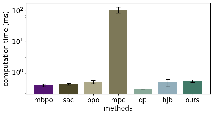
We conduct experiments on three challenging scenarios (car tracking control on different road conditions, pogobot navigation, and bipedal walker locomotion). We achieve the best performance (mean square error, failure rate, etc) compared to other baselines (MPC, RL, LQR, CLF, QP, HJB). Our learned method requires less training time than RL-based methods or the HJB approach, and at the evaluation stage, the runtime is only 1/50X1/10X the time for MPC.
Our contributions are: (1) we are the first to use a neural-network RoA estimator, planner and controller to stabilize hybrid systems \colorblackwithin certain RoA\colorblack. (2) we \colorblackdefine \colorblack a new stability for hybrid systems and derive sufficient conditions to enforce the stability with theoretical guarantees (3) our approach can be applied to different hybrid systems \colorblackeven if the dynamics is unknown\colorblack, where the controller can be state-feedback control or apex-to-apex control for periodic systems. (4) we conduct challenging experiments that involve complicated hybrid systems and outperform other baselines.
2 Related Work
Controlling hybrid systems is challenging and has been studied for decades. Various formulations for system modelling and control strategies have been extensively presented in (DeCarlo et al., 2000; De Schutter et al., 2009; Davrazos and Koussoulas, 2001; Sanfelice, 2013). We only list a few closely related works in stability analysis and controller synthesis.
Lyapunov stability analysis: The common Lyapunov function is used to prove hybrid system stability in (Dogruel and Ozguner, 1994; Fierro, 1997) . Multiple Lyapunov functions are proposed in (Peleties and Decarlo, 1992) for linear systems and (Branicky, 1998; Michel and Hu, 1999) for more general cases where the monotonous decreasing condition is relaxed. In (Malmborg, 1998), non-smooth Lyapunov functions are used for hybrid controller synthesis. For piecewise affine (PWA) systems, linear matrix inequality based approaches are proposed to construct Lyapunov certificates (Johansson, 2003; Pettersson and Lennartson, 1996). For switched systems, average dwell time (ADT) is introduced in (Hespanha and Morse, 1999; Zhai et al., 2000) to tie the stability with the ratio between stable and unstable modes. For periodic systems, Poincaré map (Clark et al., 2018) and transverse Lyapunov functions (Manchester, 2011) are used to analysis the limit cycle stability. Although equipped with theoretical guarantees for the stability, the methods above are either only suited for a specified type of systems (linear or PWA) or require expert knowledge to design the Lyapunov functions, or rely on tedious numerical methods such as Satisfiability Modulo Theories (SMT) solvers (Abate et al., 2020) and sum-of-squares (SoS) optimization (Jarvis-Wloszek et al., 2003; Topcu et al., 2008). For complicated systems, recently there is a growing trend to approximate the Lyapunov functions and the controllers using data-driven methods like Gaussian Process (Zhai and Nguyen, 2019; Xiao et al., 2020), SVM (Sun et al., 2005) and neural networks (Richards et al., 2018; Chang et al., 2019; Mehrjou et al., 2020; Dawson et al., 2022a, b). We are aligned with this and further study to stabilize hybrid systems using neural networks.
Hybrid system control designs: Upon grounding work on Lyapunov theory (Sontag, 1983; Artstein, 1983), a wide body of literature exists on synthesizing feedback controllers for switched linear and affine systems (Wicks and DeCarlo, 1997; Johansson, 1999; Mignone et al., 2000). There are also many works beyond Lyapunov controllers for more general hybrid systems, such as optimal control (Cassandras et al., 2001; Cho et al., 2001), model predictive control (MPC) (Slupphaug and Foss, 1997; Lazar, 2006; Camacho et al., 2010; Marcucci and Tedrake, 2020) and Hamilton-Jacobian reachability-based (HJB) methods (Choi et al., 2022), and region-of-attraction (RoA) based approaches (Tedrake et al., 2010; Bhounsule et al., 2018; Zamani et al., 2019). However, these methods are often computational expensive for high dimension hybrid systems. There exist reinforcement learning (RL) methods to control hybrid systems like legged robots (Benbrahim and Franklin, 1997; Morimoto et al., 2004; Neunert et al., 2020; Mastrogeorgiou et al., 2020), but finding the appropriate RL methods and rewards are extremely challenging and may cause undesired behaviors learnt to hack for high returns (Clark and Amodei, 2016). Our method shares similar philosophy with RoA-based works (Tedrake et al., 2010; Bhounsule et al., 2018; Zamani et al., 2019), whereas ours is computation-efficient, suits general nonlinear hybrid systems and can represent RoAs for arbitrary number of modes.
3 Problem Formulation
Definition 3.1 (Controlled Hybrid Systems).
A controlled hybrid system is defined as:
| (1) |
where denotes the system state, denotes the control input, and denotes the system configuration (e.g. the set point, reference velocity). The index denotes the system mode. is the flow set where states follow continuous flow map , and is the jump set where states follow discrete jump map .
We aim to stabilize the hybrid system in Def. 3.1. For each \colorblackmode of system \colorblack with equilibrium , we consider the stability defined in (Khalil, 2009). Then the sufficient conditions for \colorblackeach mode \colorblack system stability are as follows (we omit the index and the configuration for brevity).
Proposition 3.2 (Control Lyapunov Conditions for System Stability).
The system with equilibrium is asymptotically stable at if there exist a differentiable function and a control policy such that: . The is called a control Lyapunov function (CLF). The system is exponentially stable at if the further satisfies: .
The proof can be found in (Isidori, 1985)[Theorem 9.4.1]. If each \colorblacksystem mode \colorblack is stable with valid Lyapunov functions, will the hybrid system converge? Unfortunately, the answer is no with a counter-example in (Branicky, 1998). The culprit is that the system switches too fast: although the Lyapunov value is decreasing in each mode, the distance toward equilibrium is not decreasing yet. For systems with jumps, it is more unlikely to ensure the stability, as there might be jumps making infinitely often. Thus, we propose a new stability for the hybrid systems.
Definition 3.3 (Hybrid System Stability).
Given , a hybrid system is -asymptotically stable (exponentially stable), if each \colorblacksystem mode \colorblack is asymptotically stable (exponentially stable), and all states exiting the mode are within -ball of the , i.e., . We call as exiting state (and call state that enters the mode as entering state).
If is constant, the exiting states will be at most -far away from the equilibrium. If converges to zero, the sequence of the exiting states will converge to the equilibrium \colorblackhence asymptotic stability is achieved\colorblack. In this paper, we consider the former case. With constant , we define -RoA as follows.
Definition 3.4 (-Region of Attraction).
The -RoA for in mode is defined as: , where is the exiting state (for mode ) starting at .
blackUsing -RoA, we do not need to check dwell time conditions like (Hespanha and Morse, 1999)\colorblack. To efficiently check if -RoA, \colorblackwe seek a set representation for -RoA and a scalar function/index to tell whether is in the set\colorblack. We use Lyapunov level set to (conservatively) represent -RoA.
Definition 3.5 (Maximum -Stable Level Set).
For mode and configuration , the largest level set within -RoA is called Maximum -Stable Level Set, and is called Maximum -Stable Level Set index.
For an entering state , we have -RoA. One step ahead, at mode with switching , it requires . Propagating from to , we derive sufficient conditions for hybrid system stability proved in 111The appendix is at https://mit-realm.github.io/hybrid-clf/static/appendix.pdf(Meng and Fan, 2022)[Appx. A].
Theorem 3.6 (Lyapunov Conditions for Hybrid System -Stability).
A hybrid system in Def. 3.1 is -exponentially stable, if there exists a Lyapunov function for each mode (and configuration ) satisfying all conditions in Prop. 3.2 and , and for each entering state that moves toward the mode , we have the to satisfy:
| (2) |
where , and , are the maximum -stable level set indices for modes and , and is the local Lipschitz constant for function within -ball of .
In short, Theo. 3.6 guarantees each \colorblacksystem mode \colorblack is exponentially stable, and at switching , the entering state is within -RoA for mode , and the next entering state is also inside -RoA for mode . The Lipschitz constant can be approximated by at for small . In the next section, we will use neural networks to satisfy Theo. 3.6 for hybrid system stability.
4 Methodology
To control the system in Def. 3.1, we propose a learning framework in Algor. 1. Guided by Theo. 3.6, we first learn the controller and the CLF to stabilize the \colorblacksystem \colorblack within each mode. Then we perform the RoA estimation, and finally, we bring in the differentiable planner that leverages the controller and RoA estimator to enforce the hybrid system stability.
4.1 Learning neural Lyapunov functions and controllers
We train neural networks (NN) to synthesize the control Lyapunov functions and controllers for each \colorblacksystem mode\colorblack. During training, we use the controller to roll out trajectories from uniformly sampled initial states and compute the CLF values. To satisfy the CLF conditions in Theo. 3.6, we design the Lyapunov function as , where is an NN that takes as input and outputs a matrix, and is an NN taking as inputs and outputs a scalar. In this way, the positive definiteness and the norm inequalities of the Lyapunov functions are naturally satisfied. Finally, to enforce the Lyapunov value decreasing (exponentially) along the trajectories , we design the loss:
| (3) |
where and we compute the derivative term .
4.2 Learning neural RoA estimator
After training for the CLF and controllers, we estimate the maximum -stable level set in Def. 3.5 for any given using: , where is the -RoA in Def. 3.4. For each , we set and uniformly sample initial states, roll out trajectories and find the largest Lyapunov value for all the initial states that have exiting states within the -ball of the equilibrium. We train the NN RoA Estimator with:
| (4) |
where is the set for simulated trajectories and maximum -Stable level set indices. In this way, the RoA under configuration can be approximated by .
4.3 Differentiable configuration planner
We use a differentiable planner to ensure switching stability by satisfying the last condition in Eq. 2 of Theo. 3.6. Assume is given at mode . We use gradient descent to find to minimize:
| (5) |
where and . It is time-consuming to evaluate , and for each and . Empirically, we set =0.9 and = for = (ablation in (Meng and Fan, 2022)[Appx. F]). The optimization converges after 310 steps, adding only little runtime overhead. We can also use a new loss for periodic systems with decomposable jump map (common in error-state dynamics):
| (6) |
where the heuristic is to guide the configuration gradually approaches the target configuration :
| (7) |
We guarantee it converges to the target in finite steps (proved in (Meng and Fan, 2022)[Appx. B]):
Theorem 4.1 (Finite-step converging toward the target configuration).
Whilewhiledo \SetKwForForAllforeachdo \SetKwProgFnFunction
Sample from the hybrid system in Def. 3.1 \tcp*Training phase
for all , do Train and with the loss in Eq. 3
Initialize state , mode and time \tcp*Testing phase
while do \uIf right before entering mode (with next mode )
\uElse ,
fig:env
\subfigure[Car tracking control] 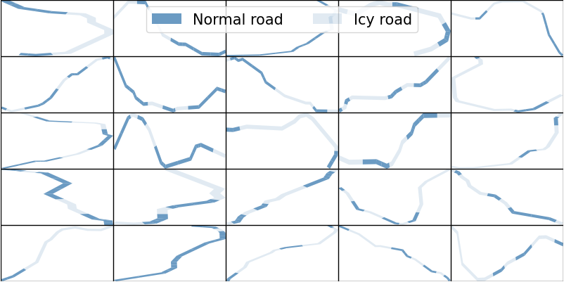 \subfigure[Pogobot navigation]
  \subfigure[Bipedal gait tracking]
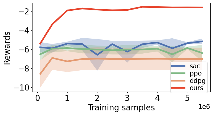
  \subfigure[Car control reward]
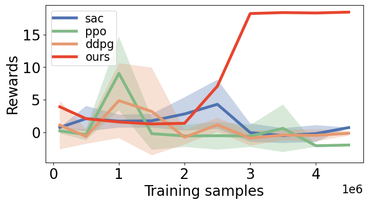
  \subfigure[Pogobot reward]
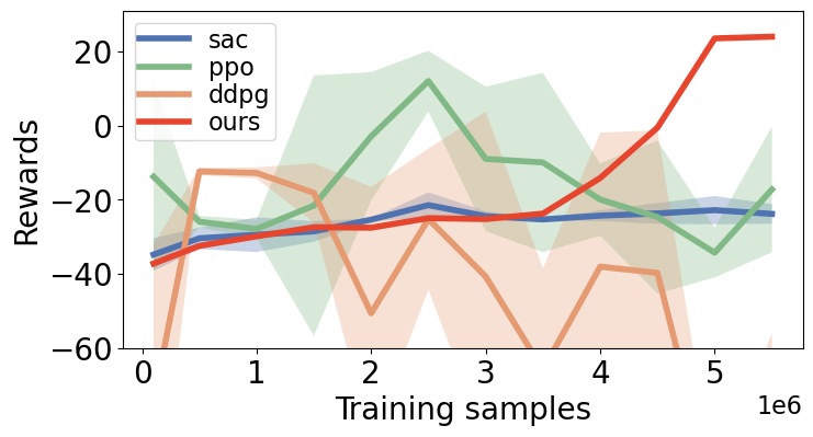
  \subfigure[Bipedal walker reward]
5 Experiments
fig:car-roa-comparisons
\subfigure[RoA] 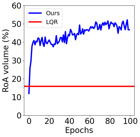 \subfigure[x-y plane]
  \subfigure[v- plane]
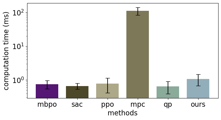
We conduct three challenging experiments shown in Fig. LABEL:fig:env. Our method achieves the best performance (success rate, RMSE, etc) than most baselines and is 1050X faster than MPC. Our approach also results in shorter training time (0.5X of RL methods and 0.1X of HJB approaches). Baselines: For all cases we compare with: model-base RL (MBPO (Janner et al., 2019)), model-free RL(SAC (Haarnoja et al., 2018), PPO (Schulman et al., 2017) and DDPG (Lillicrap et al., 2015)) and model predictive control (MPC). Besides, for the car case, we compare with Linear Quadratic Regulator (LQR) and single CLF (Chang et al., 2019). For the bipedal we compare with quadratic program (QP) and Hamilton-Jacobian (HJB) (Choi et al., 2022). We did not compare with HJB for (9-dim) car or (8-dim) pogobot as the state dimension is too high for HJB to handle. Implementation details: For CLF, the controller and the RoA estimator, we use 2-layer NNs with 256 units in each layer and ReLU (Nair and Hinton, 2010) in intermediate layers. The controller uses TanH (LeCun et al., 2012) in the last layer to clip the output in a reasonable range. We implement our method in PyTorch (Paszke et al., 2019). The training takes 36 hours on an RTX2080 Ti GPU. More details are in (Meng and Fan, 2022)[Appx. E].
Remarks on sample efficiency: As shown in Fig. LABEL:fig:env, compared to RL under the same sample size, we achieve the highest rewards. This is because RL directly interacts with the hybrid systems, whereas ours learns to control the \colorblacksystem \colorblack under each mode, which is easier.
fig:car-comparisons
\subfigure[Lane deviation] 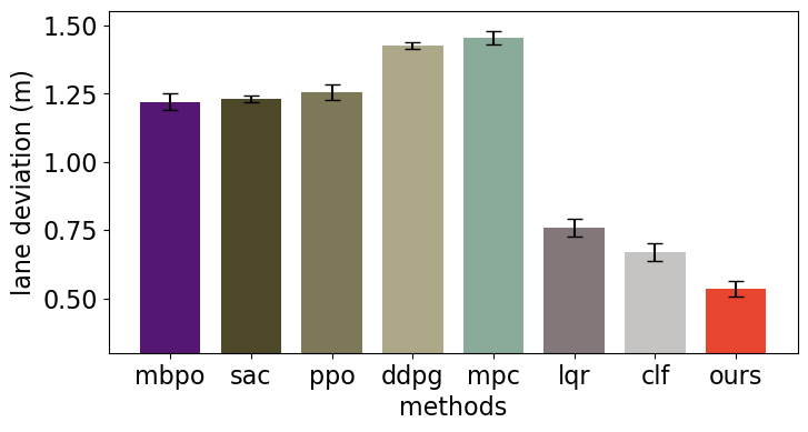 \subfigure[Mean square error]
  \subfigure[Distance to goal]
  \subfigure[Computation time]
  \subfigure[T=2.5s]
  \subfigure[T=3.8s]
  \subfigure[T=5.8s]
5.1 Car control under different road conditions
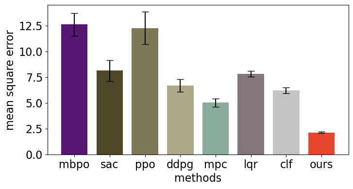
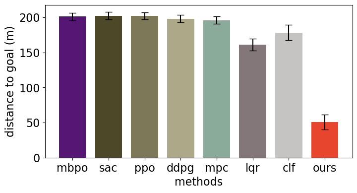
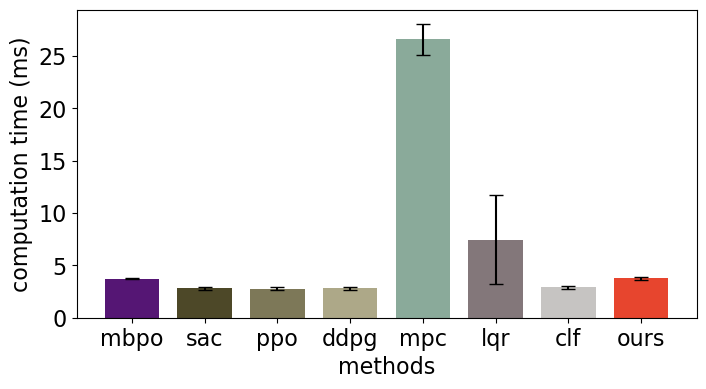
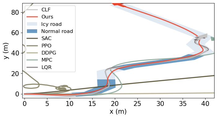
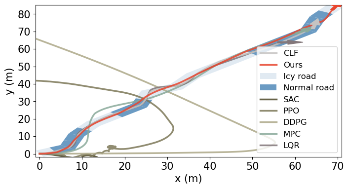
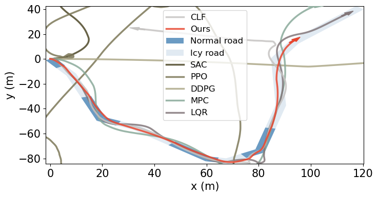
We consider the tracking control problem for the single-track model in (Althoff et al., 2017) under varied frictions. The system is hybrid as varied frictions and tracking velocities lead to different dynamics. The challenge is that when the friction is low (e.g., on icy roads), the road cannot provide enough traction to keep the car on the lane. To stabilize the system, the controller needs to track proper configurations (speeds and waypoints). Our method ensures the entering state at the connection of segments is always in the RoA of the next segment. Setups: We generate 25 maps with 10 randomly sampled segments. Each segment has friction and length . The angle between consecutive segments . Metrics: We measure average lane deviation, mean square error (MSE) to the reference trajectory, distance to the goal (before driving out of lane), and the run time per step.
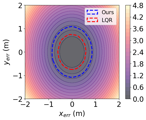
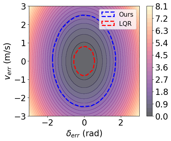
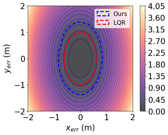
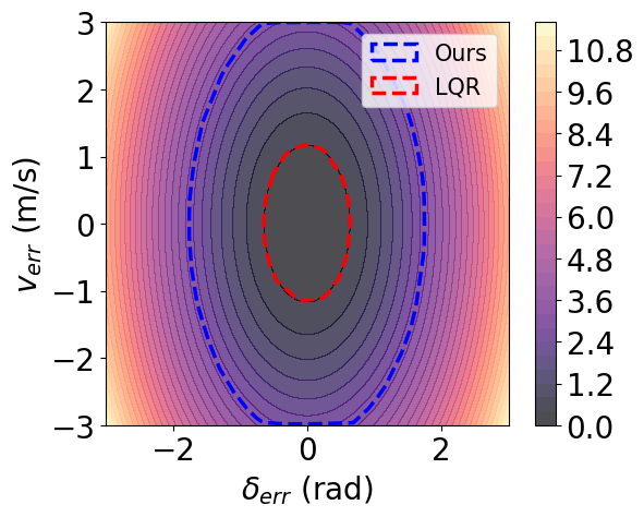
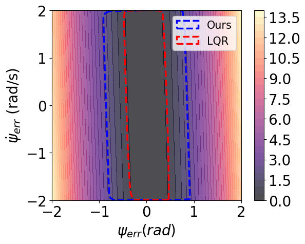
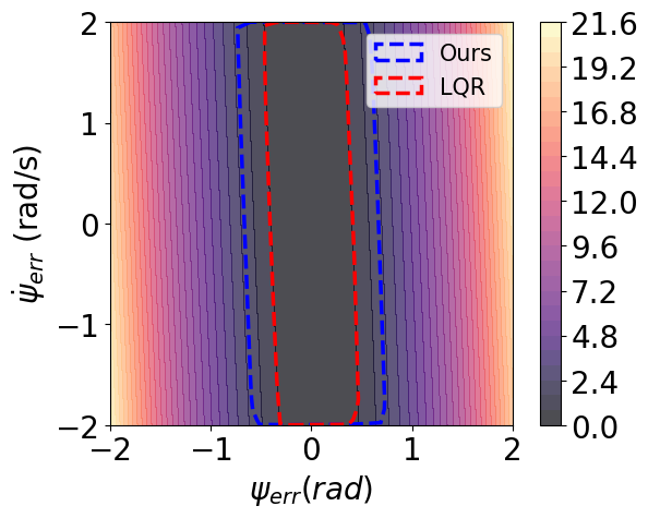
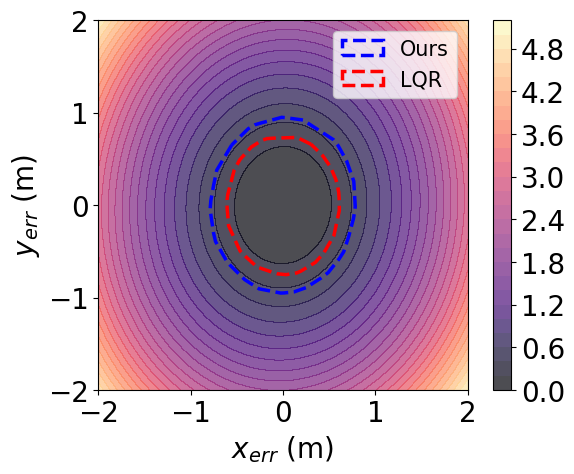
As shown in Fig. LABEL:fig:car-roa-comparisons(a), the RoA of our approach surpasses the LQR method in just a few epochs and converges in 100 epochs, becoming nearly 2X larger than the LQR RoA. From the RoA visualization in Fig. LABEL:fig:car-roa-comparisons(b, c), we show that the gain is mainly from velocity error, tire angle error, longitudinal and lateral errors. This shows our method can enlarge the RoA to stabilize more states. The rest visualizations can be found in (Meng and Fan, 2022)[Appx. I].
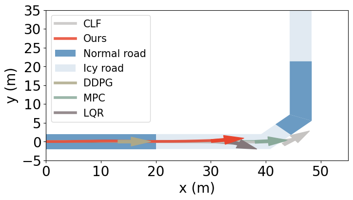
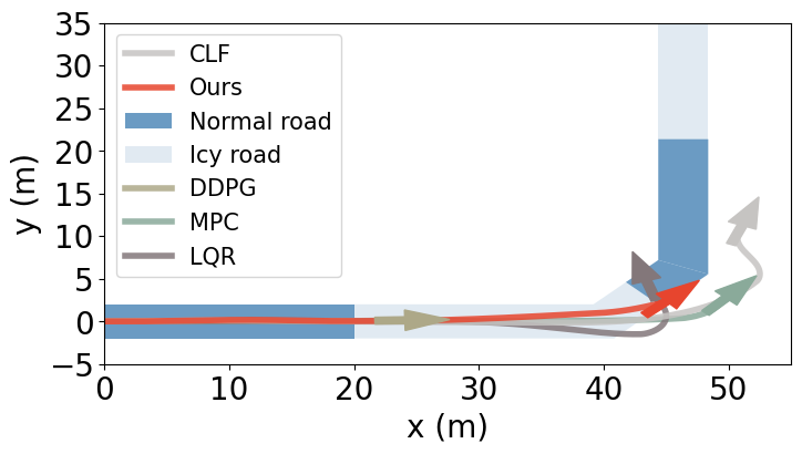
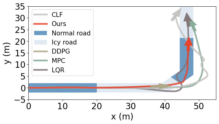
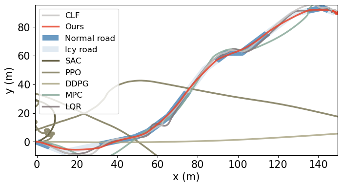
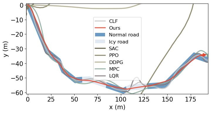
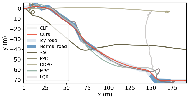
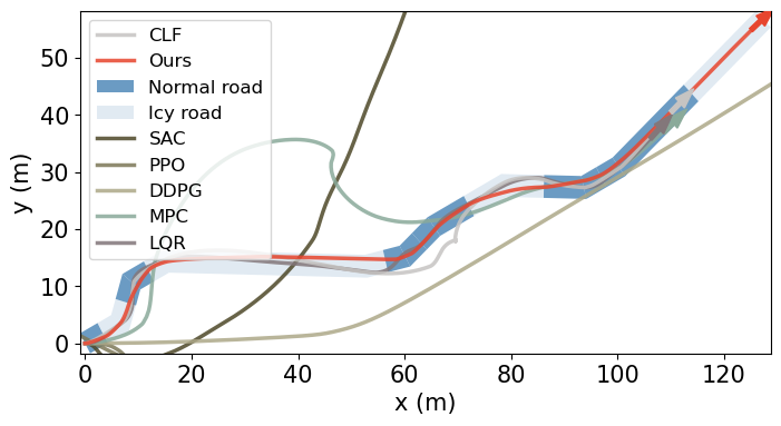
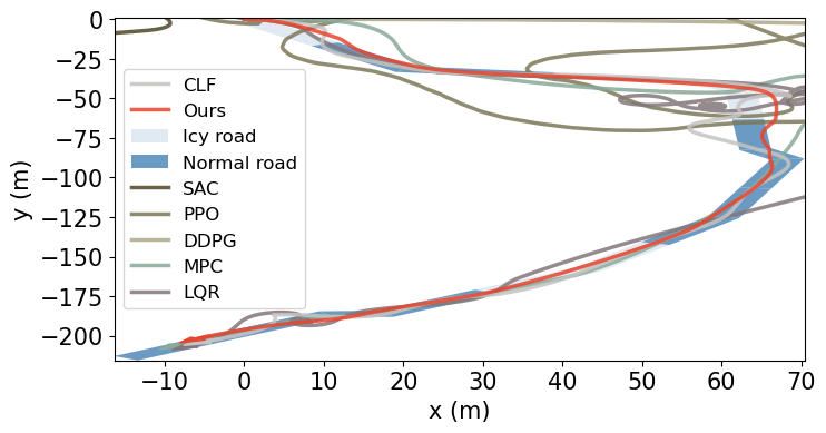
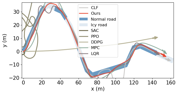
Next, we compare with other baselines. As shown in Fig. LABEL:fig:car-comparisons, we achieve the lowest lane deviation and MSE, 67%75% reduction in the distance to goal, and low run time on par of RL, which is less than 0.1X of the time used by MPC. Qualitatively, as shown in Fig. LABEL:fig:car-comparisons (here we omit MBPO, SAC and PPO because they cannot provide reasonable trajectories), our approach is the only method that can keep the car on the road. The reason is that our method learns to decelerate and turn left to prepare for the next icy road segment (Fig. LABEL:fig:car-comparisons(a)), so that the car can gain more traction on the icy road for a normal left turn (Fig. LABEL:fig:car-comparisons(b)) where other methods fail to keep the car on the road (Fig. LABEL:fig:car-comparisons(c)).
fig:pogo-comparisons
\subfigure[Velocity error] 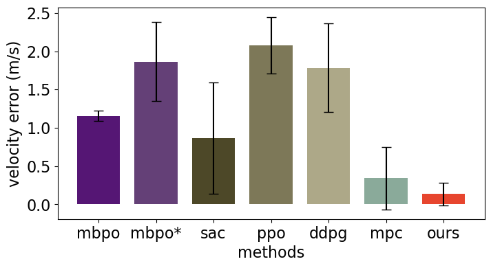 \subfigure[Distance to goal]
  \subfigure[Collision rate]
  \subfigure[Runtime]
  \subfigure[RL method (DDPG)]
  \subfigure[RL method (PPO)]
  \subfigure[MPC method]
  \subfigure[Our approach]
5.2 Pogobot navigation
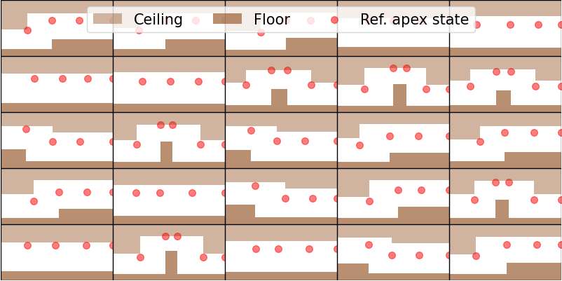
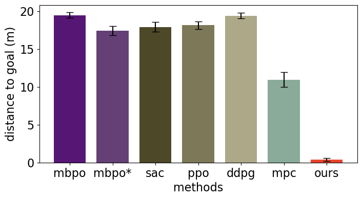
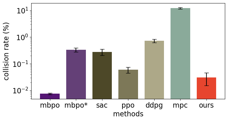
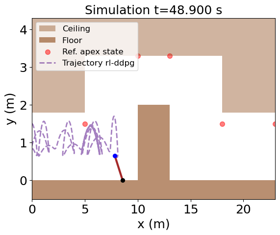
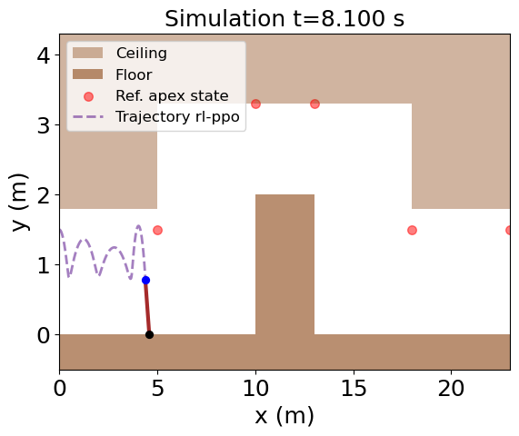
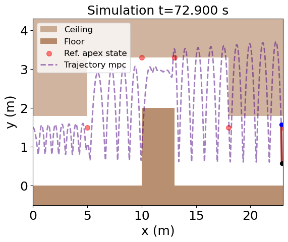
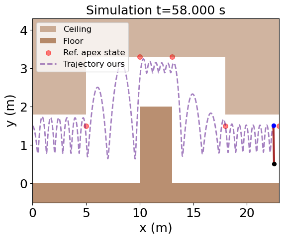
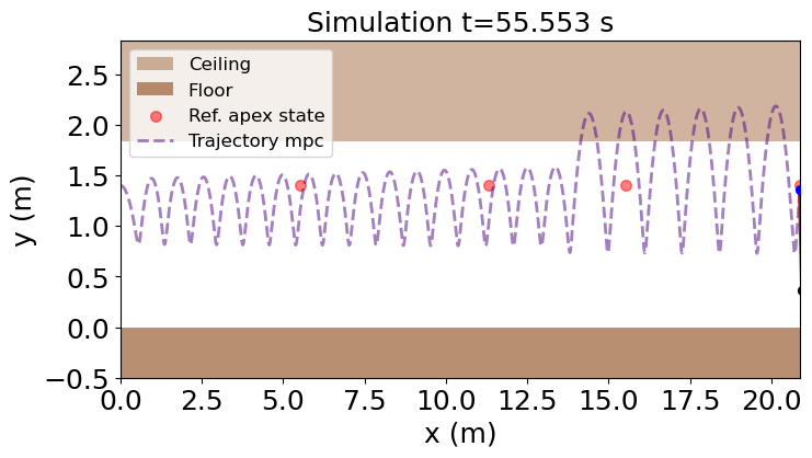
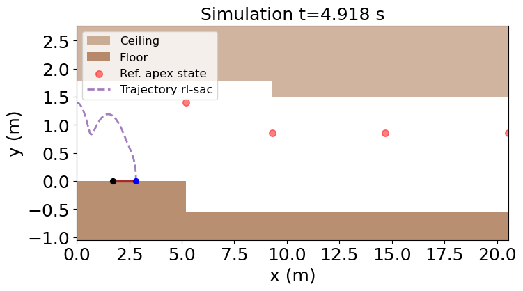
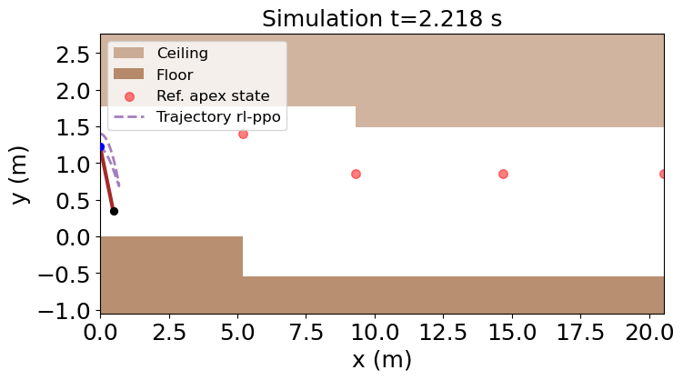
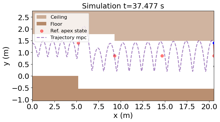
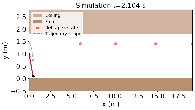
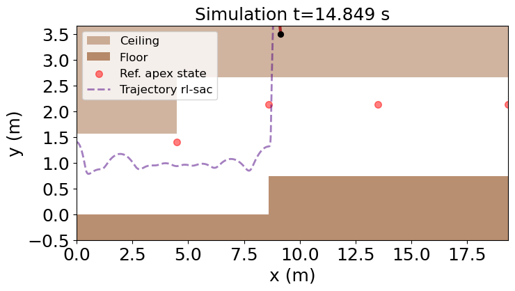
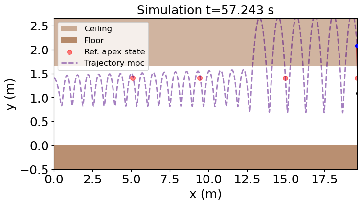
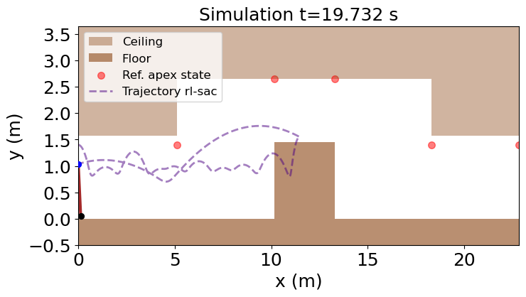
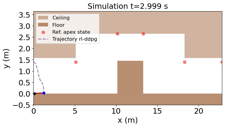
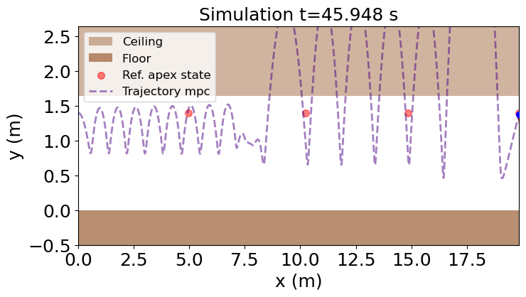
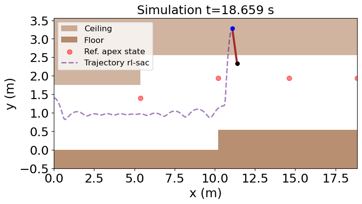
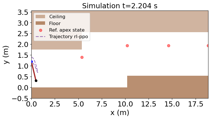
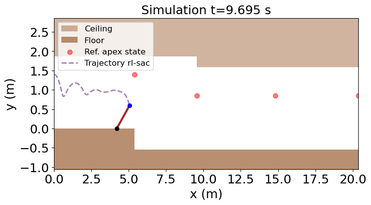
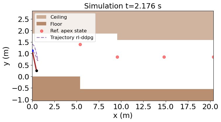
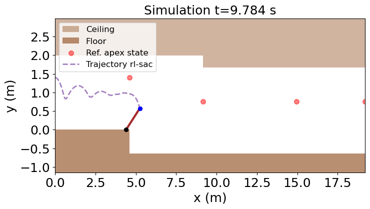
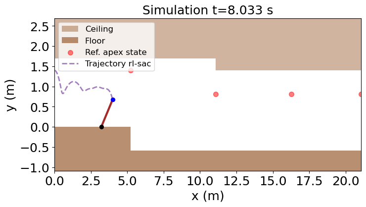
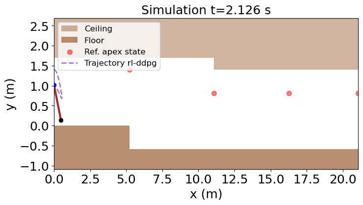
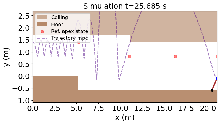
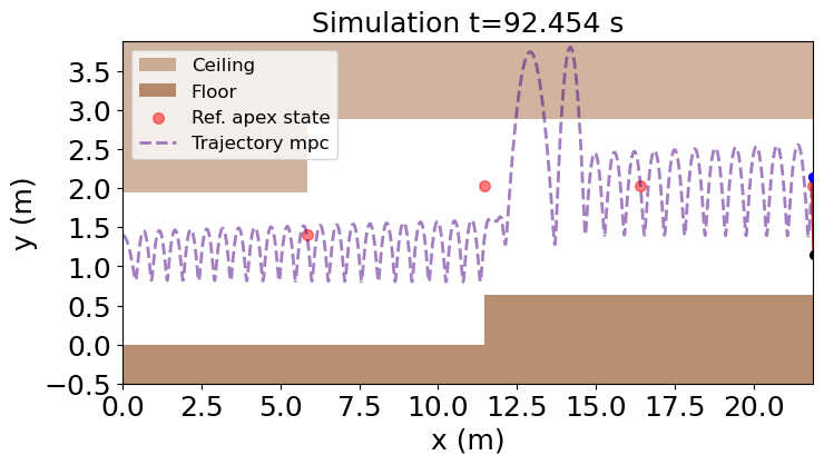
We control a pogobot (with the model in (Zamani et al., 2019)) to jump through 2d mazes shown in Fig. LABEL:fig:pogo-comparisons. The pogobot alternates between flight and stance phases. The apex state is when the pogobot is at the top of a trajectory in the flight phase. Given the reference apex states, the goal is to jump through the maze safely. Our method \colorblackfirst learns the unknown apex state dynamic then \colorblack plans configurations (reference apex state) to ensure apex states are within the RoA of the next reference apex state. Setups: We generate 25 maps by randomly sampling 35 segments with a segment length , a floor height , a ceiling height , and a reference speed . Metrics: We measure the velocity error, the remaining distance to goal, the collision rate, and the computation runtime.
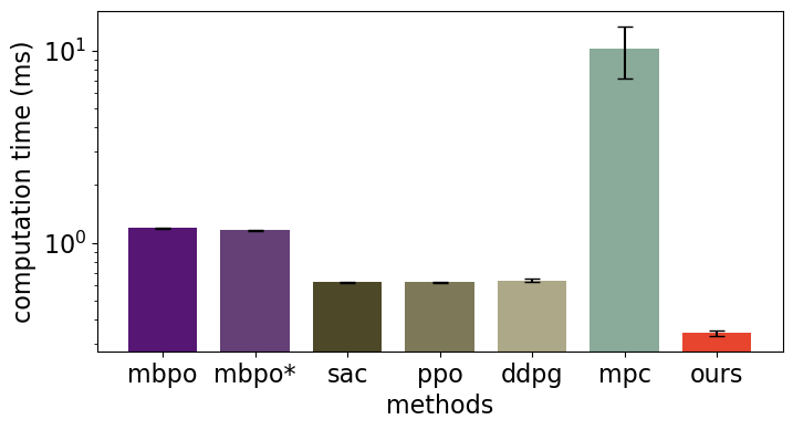
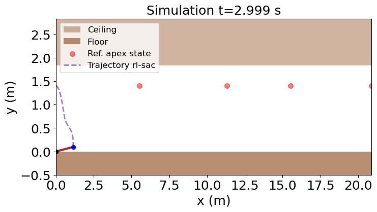
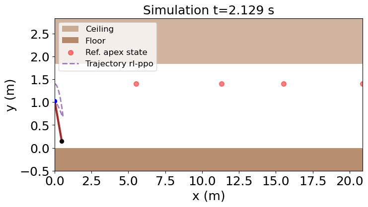
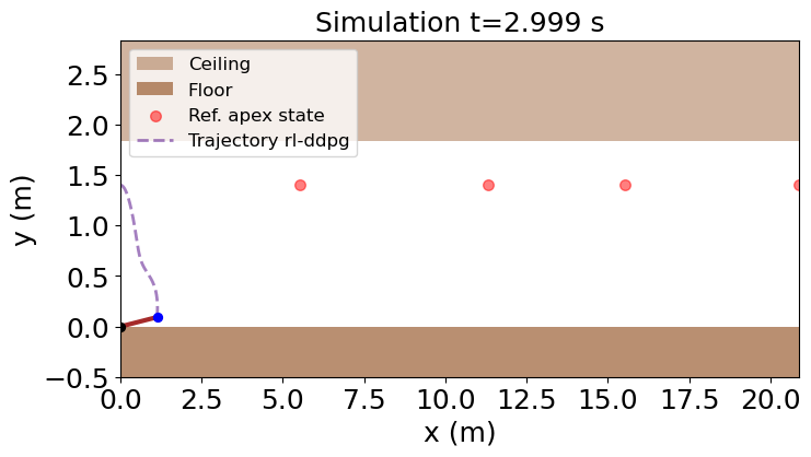
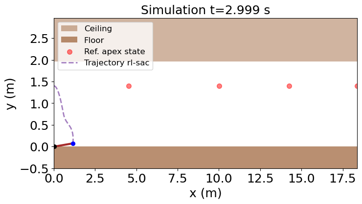
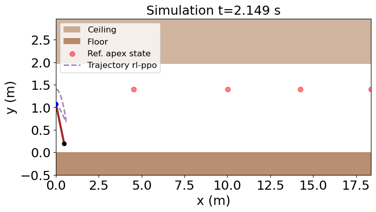
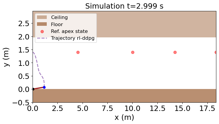
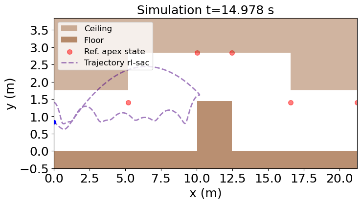
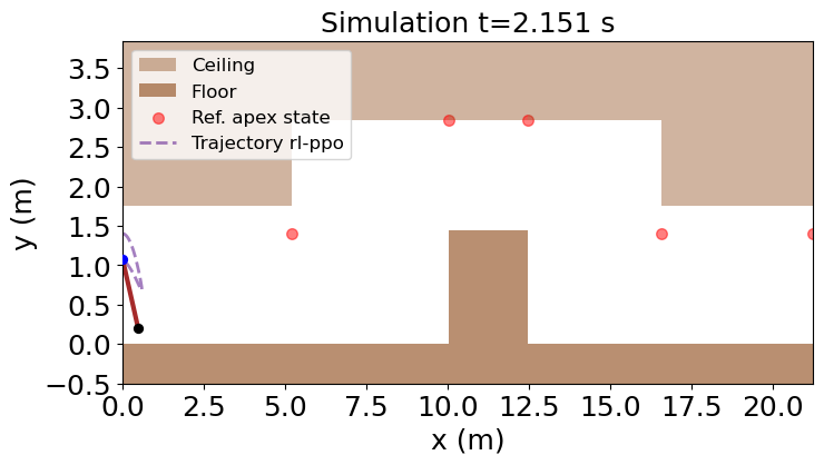
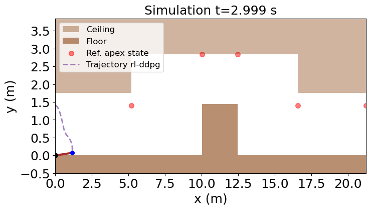
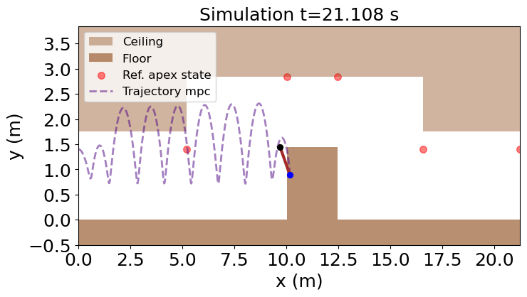
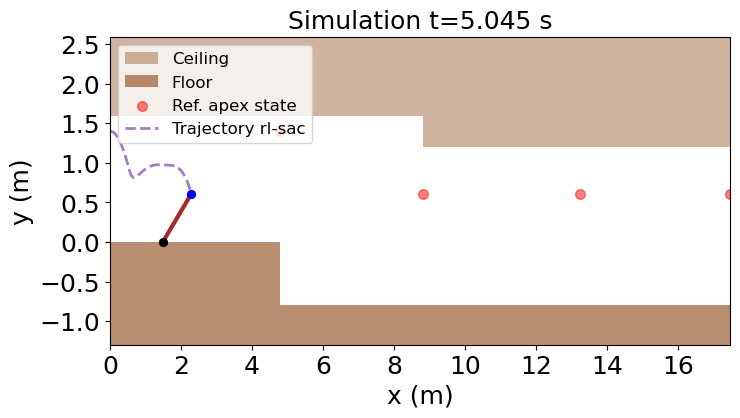
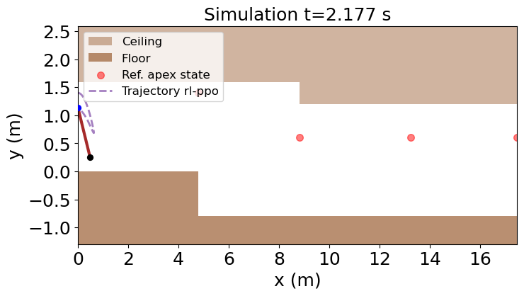
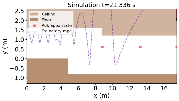
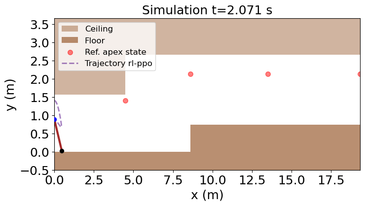
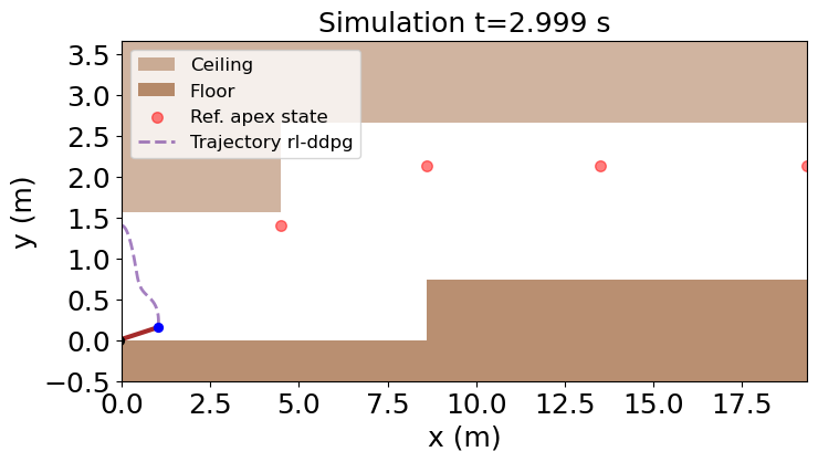
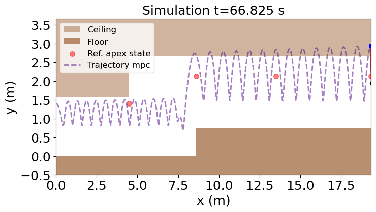
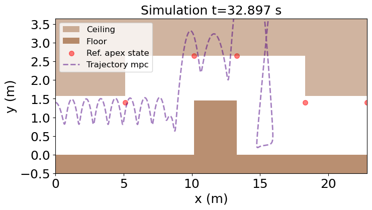
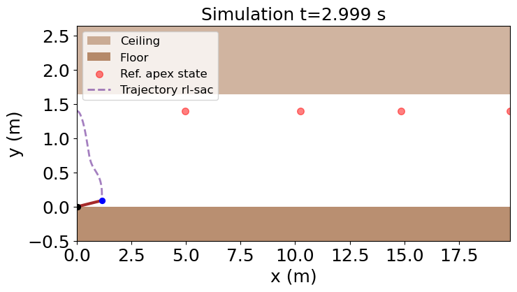
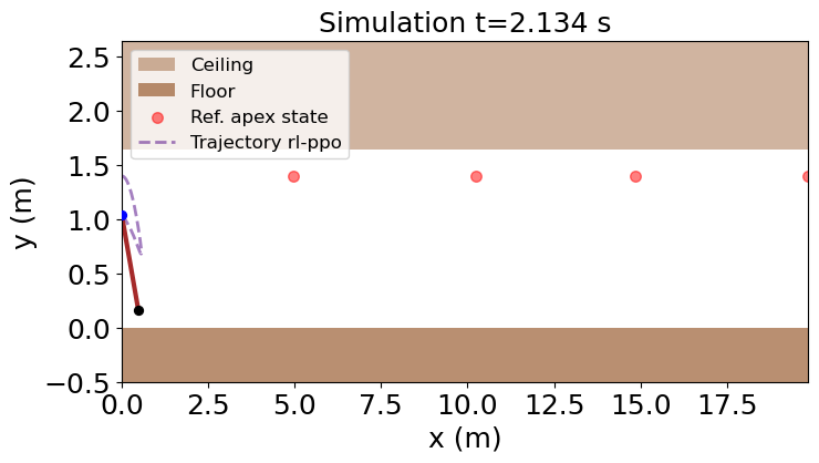
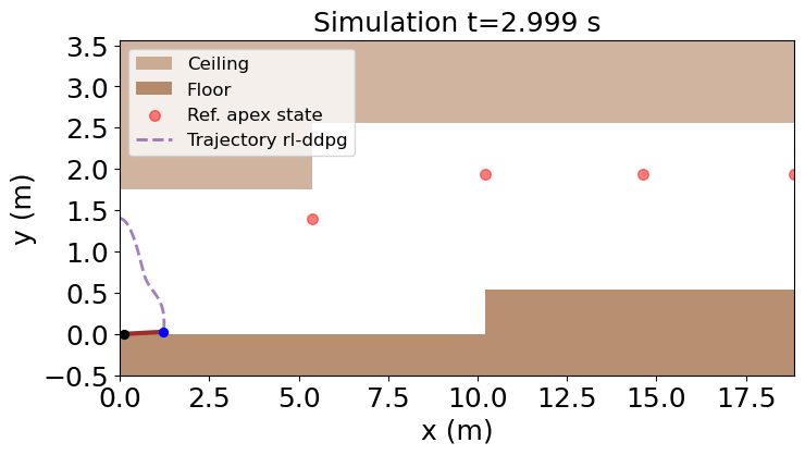
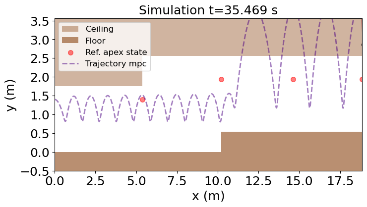
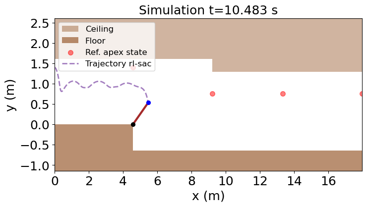
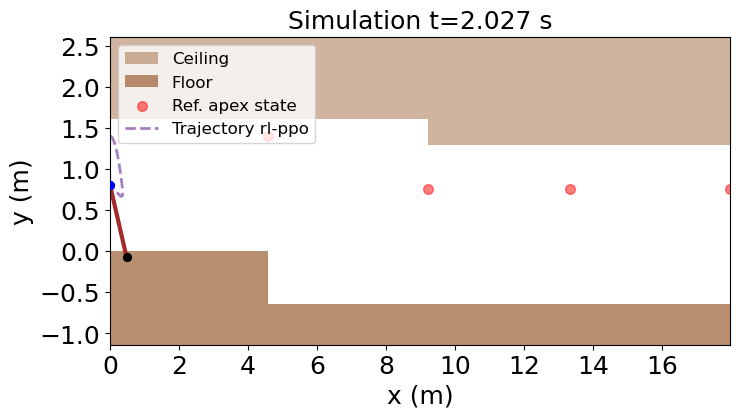
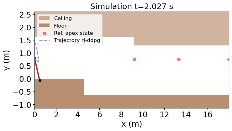
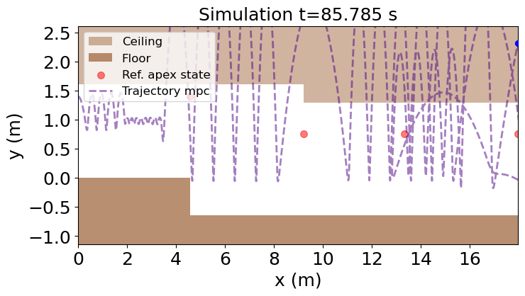
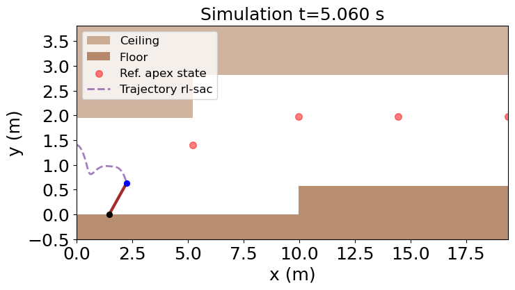
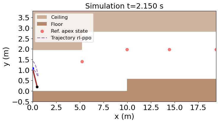
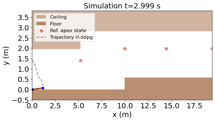
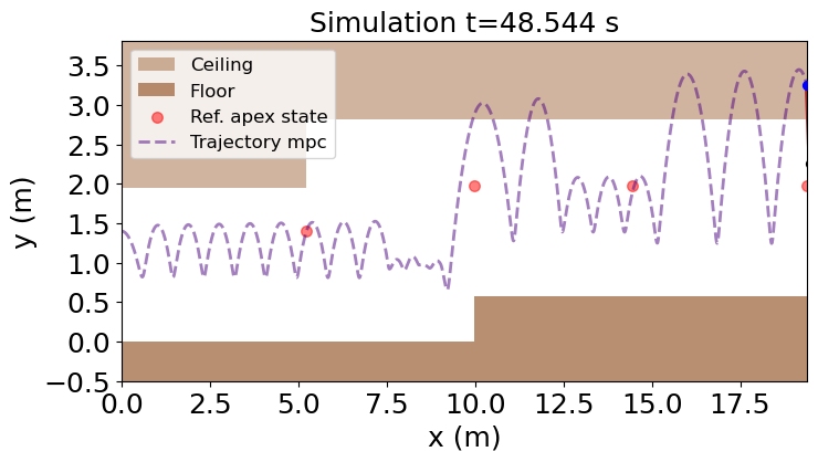
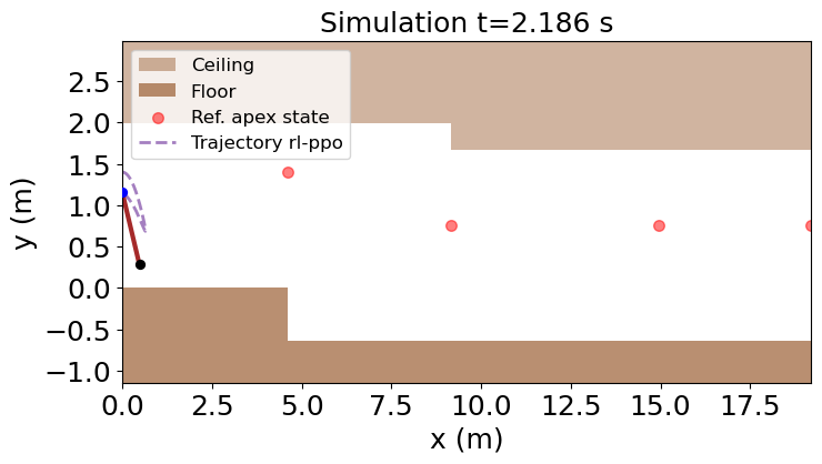
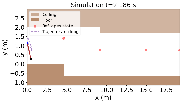
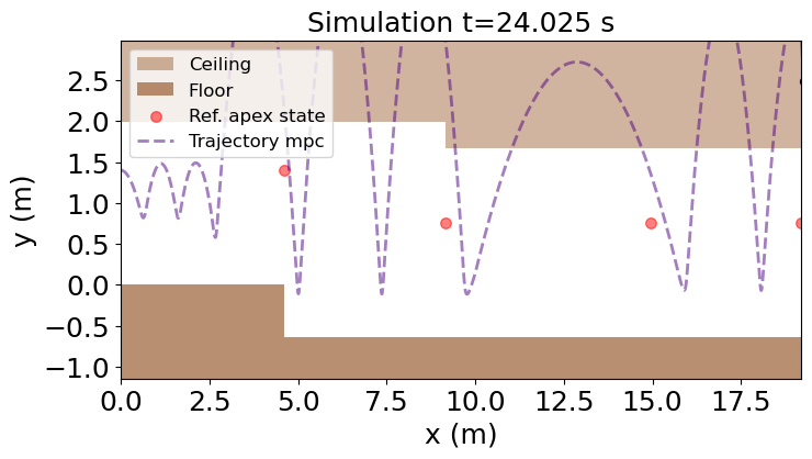
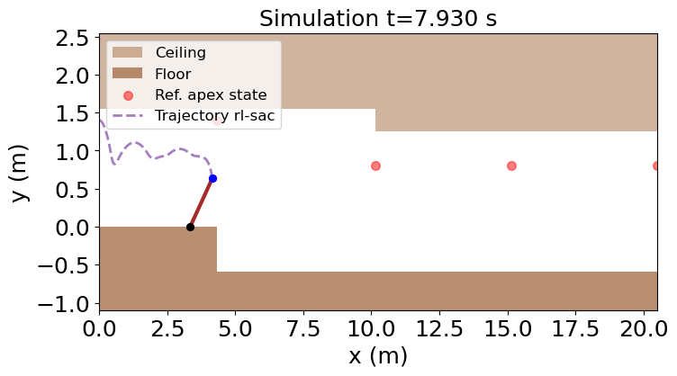
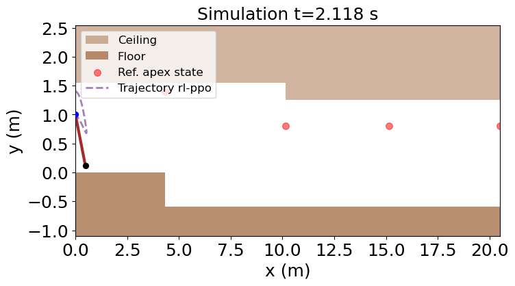
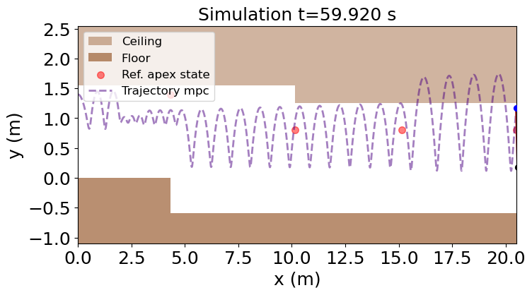
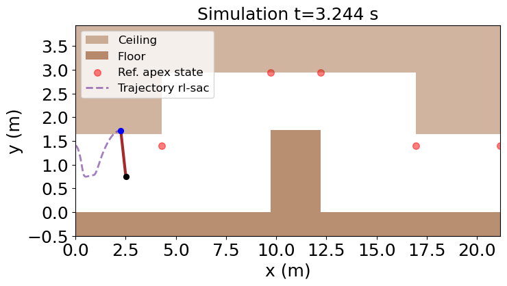
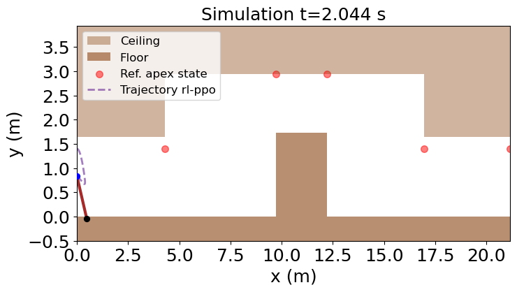
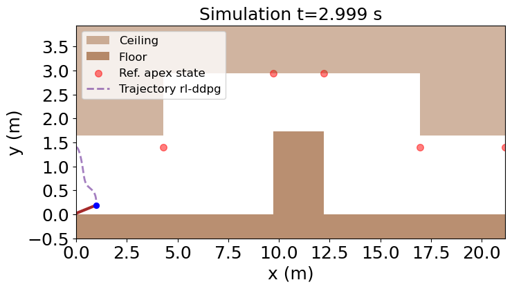
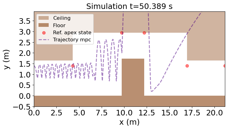
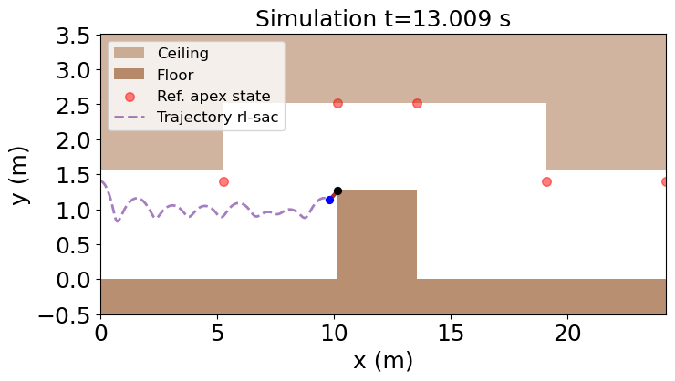
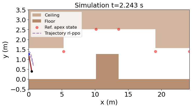
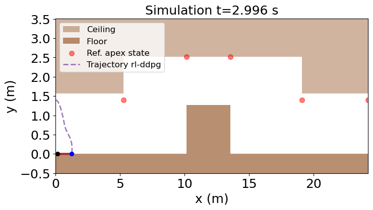
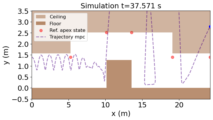
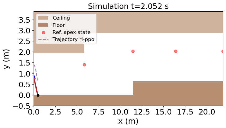
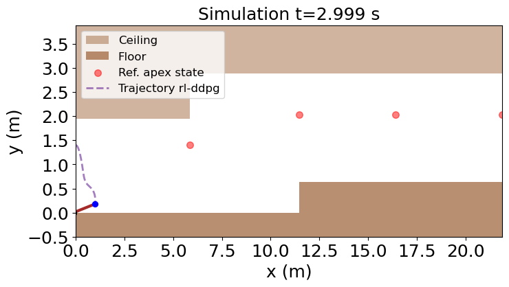
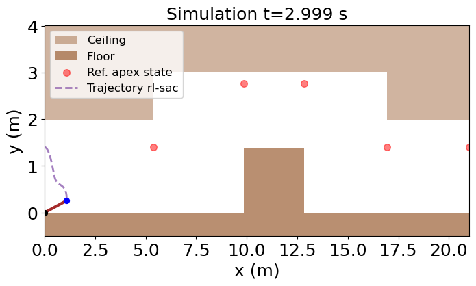
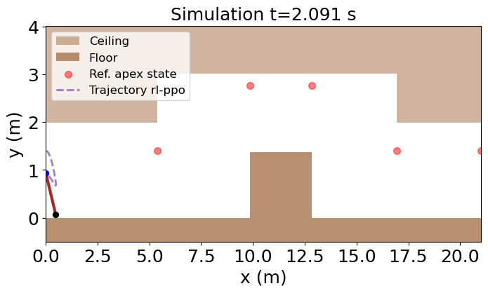
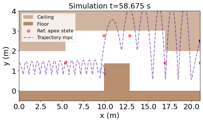
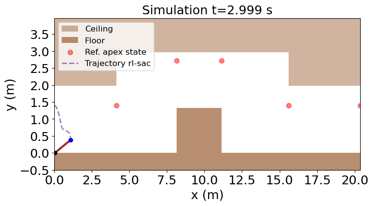
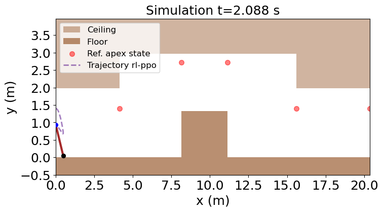
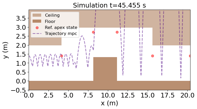
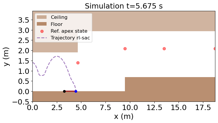
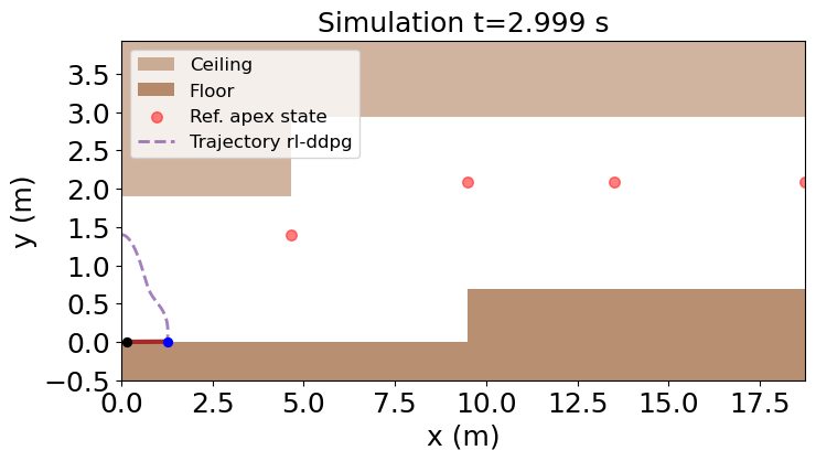
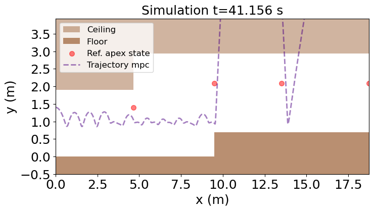
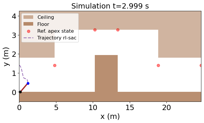
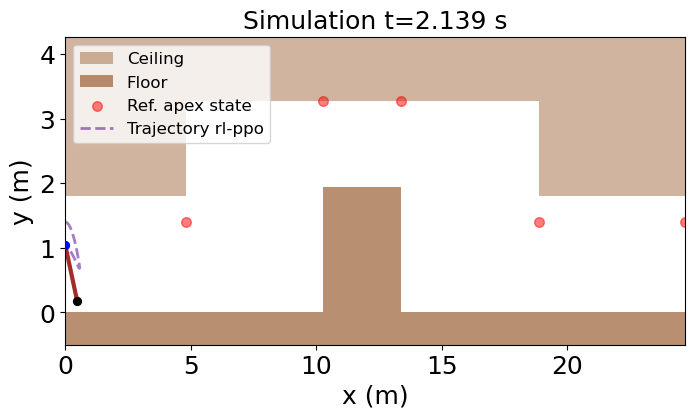
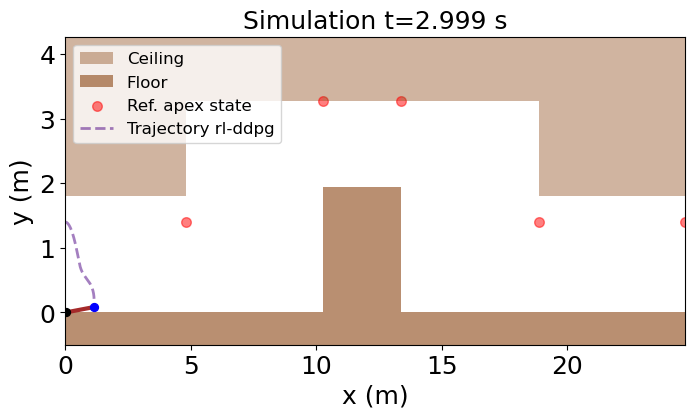
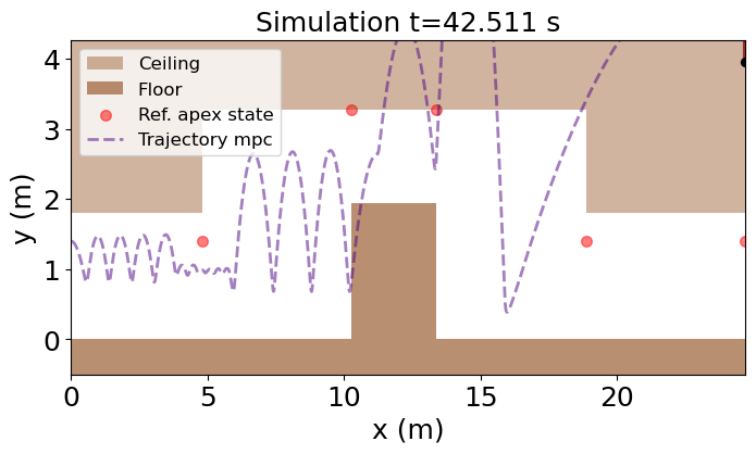
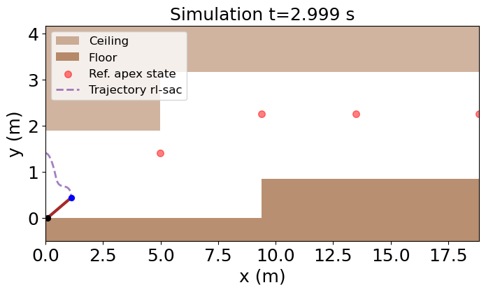
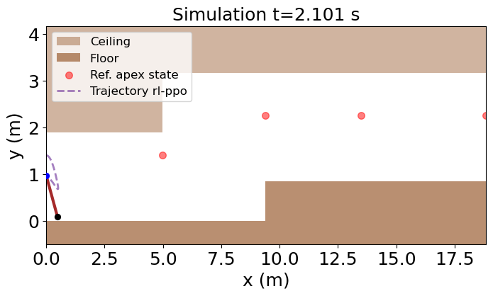
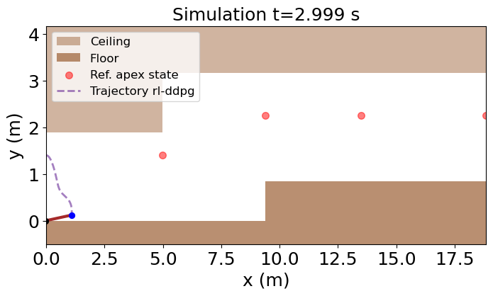
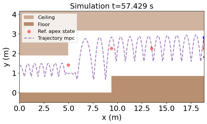
Since we use a learned dynamics in this case, we also compare with MBPO with pretrained dynamic model learnt from our approach (denoted as ). As shown in Fig. LABEL:fig:pogo-comparisons, our approach achieves the lowest velocity tracking error, remaining distance to goal, low collision rate and computation time (MBPO achieves the lowest collision rate as it often jumps out of valid region before crashing - which explains its high distance-to-goal metric). Our approach uses just 1/70X of the computation time as needed for MPC. The simulation in Fig. LABEL:fig:pogo-comparisons shows that ours is the only approach to safely jump through the 2d maze, whereas DDPG and PPO methods start to jump to the left afterwards (here we omit the SAC result because it cannot plan for one cycle), and MPC method results in collisions. More details can be found in (Meng and Fan, 2022)[Appx. CD].
fig:bipedal-comparisons
\subfigure[RMSE] 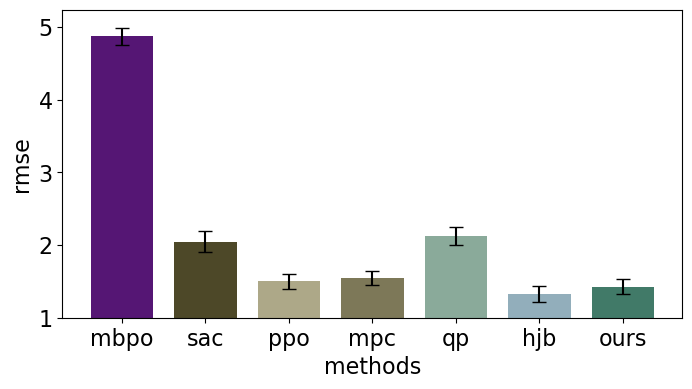 \subfigure[Failure rate]
  \subfigure[Invalid rate]
  \subfigure[Computation time]
  \subfigure[RMSE]
  \subfigure[Failure rate]
  \subfigure[Invalid rate]
  \subfigure[Computation time]
5.3 Bipedal walker locomotion
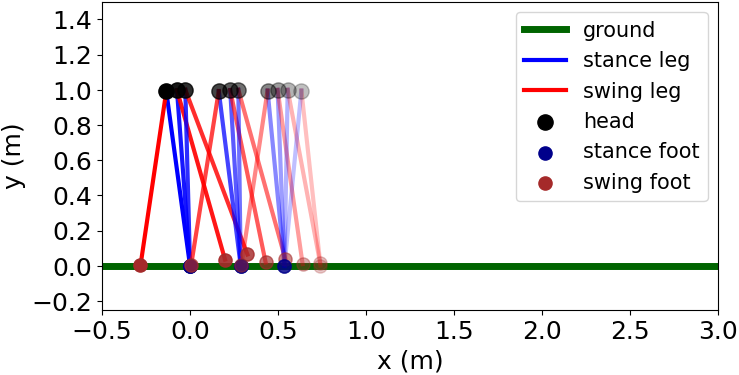
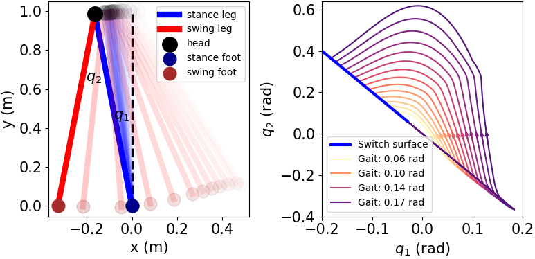
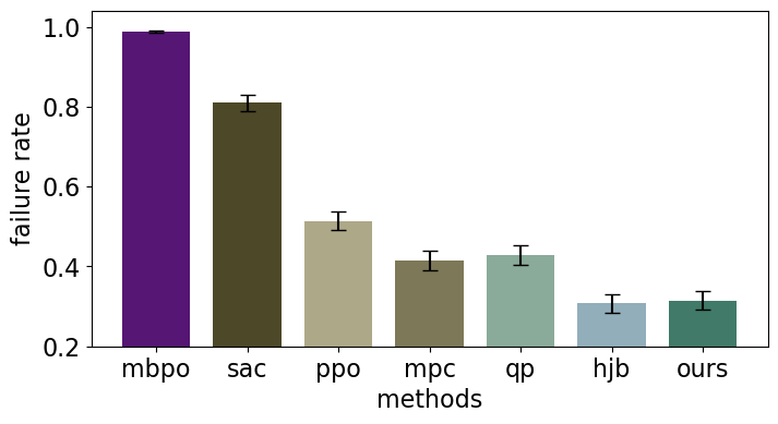
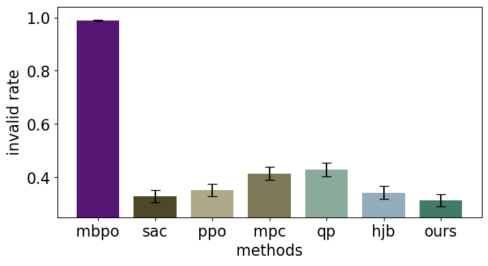
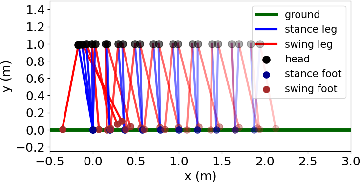
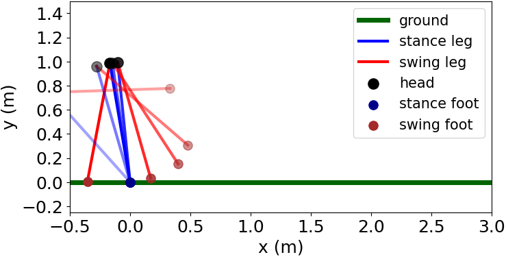
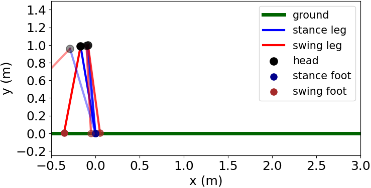
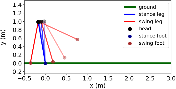
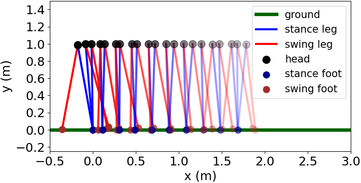
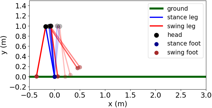
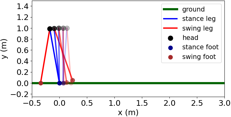
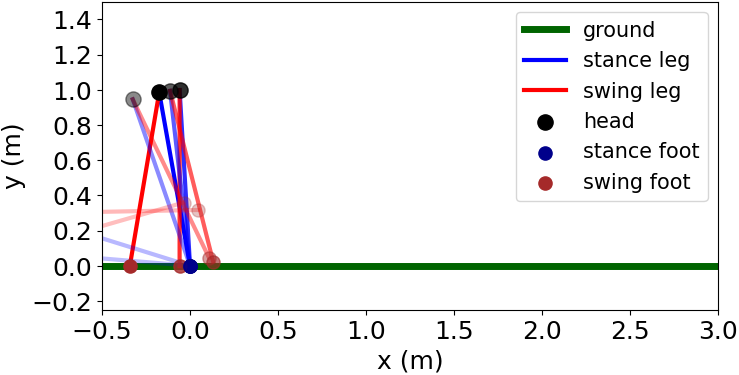
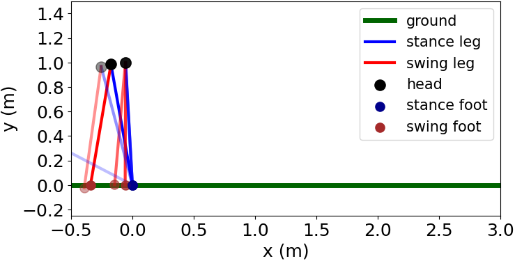
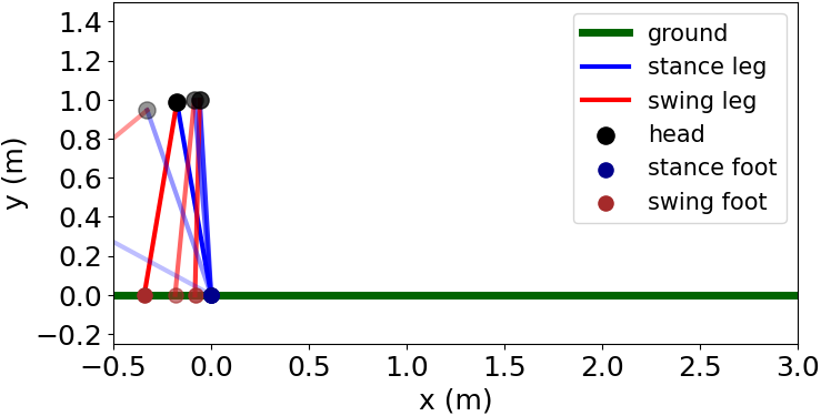
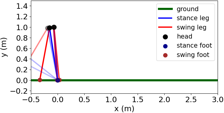
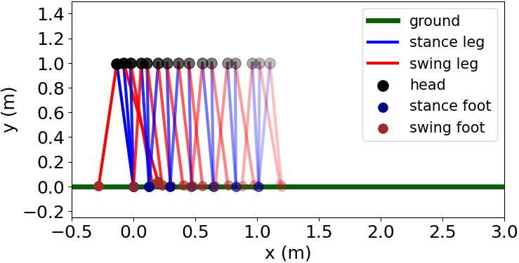
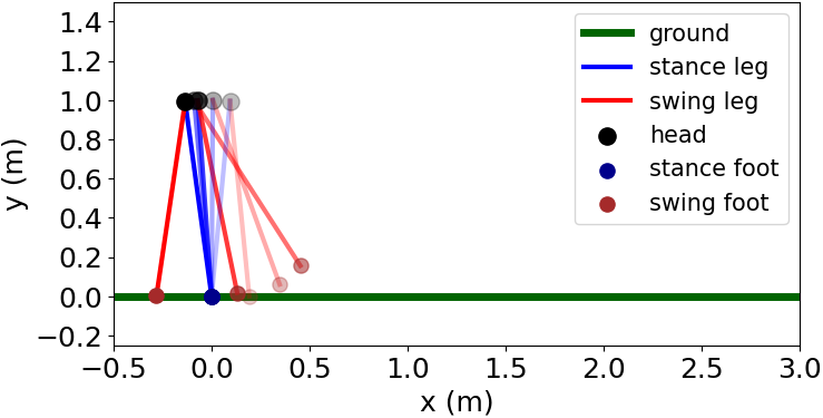
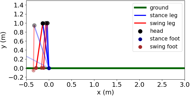
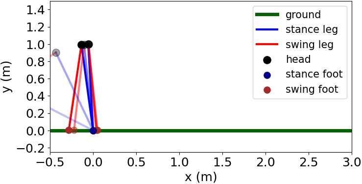
We control the bipedal robot (Choi et al., 2022) to converge to a target gait. The configuration here is the leg angle of the next gait at the switch surface shown in Fig. LABEL:fig:env(c). It is hard to converge directly to the goal gait when the initial gait is far away. Thus, we use the loss in Eq. 7 in planning to ensure the gait at each switching is closer to the target gait and our controller guarantees the state converges to the intermediate gait. Setups: We calculate the gaits using Frost Library (Hereid and Ames, 2017), uniformly sample the initial states around each gait with angle and target gait . When compared to HJB, we set the target gait0.13 since HJB only handles that gait. We compare other baselines with different target gaits. Metrics: We measure RMSE towards reference gaits, failure rate for convergence, invalid trajectories rate and run time.
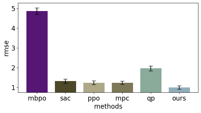
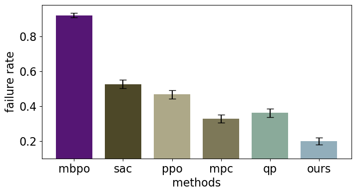
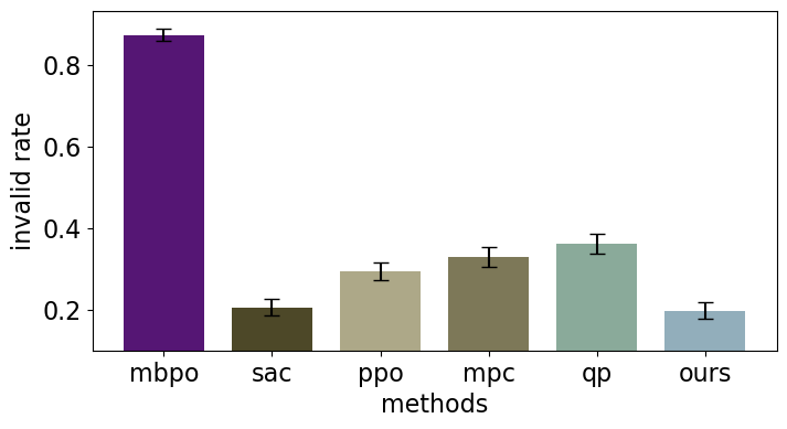
As shown in Fig. LABEL:fig:bipedal-comparisons(a)-(d), our approach achieves the closest RMSE, failure rate, and invalid trajectory rate to HJB approach. The third best method for failure rate is MPC, which takes a much longer computation time. MBPO has the worst performance probably due to the complicated dynamics which is hard to learn. Compared to HJB, our advantage is in the quick adaptation to other targeted gaits. Trained in less than 6 hours, our method can also learn to converge to other target gaits, whereas the learning time for the HJB method to converge to one target gait is 36 hours. We compare our method with other non-HJB approaches for converging to different gaits. As shown in Fig. LABEL:fig:bipedal-comparisons(e)-(h), we achieve the lowest RMSE, failure rate, invalid rate, and low running time.
5.4 Limitations
Firstly, the RoA estimation is after the controller training, thus a refinement for the RoA estimator is needed if the controller is updated. One thought is to design a “robust” RoA estimator that can tolerate mild changes in controller parameters. Besides, since the certificates are NNs with limited amount of neurons, we cannot guarantee the certificates being satisfied in the whole state space. Also we might bring in errors when numerically approximate the continuous dynamic, though we show in (Meng and Fan, 2022)[Appx. F] that the performance is consistent across varied . In addition, we assume we can obtain full information for the system state and assume no disturbances or noises, which might not hold in real-world experiments. We aim to solve these in future works.
6 Conclusion
We propose a learning-based hierarchical approach to stabilize nonlinear hybrid systems. The learned low-level controller can stabilize the system states within each mode. Upon switching, the high-level planner finds the optimal configuration that guarantees the next entering state is within the RoA of the next mode. Experimental results show that our approach achieves the best overall performance on multiple hybrid systems compared to other approaches. For future works, we aim to tackle some of the limitations discussed in Sec. 5.4, and extend this framework to further control hybrid systems with perception modules and the presence of estimation error and disturbances.
Acknowledgement
The Defense Science and Technology Agency in Singapore and the C3.ai Digital Transformation Institute provided funds to assist the authors with their research. However, this article solely reflects the opinions and conclusions of its authors and not DSTA Singapore, the Singapore Government, or C3.ai Digital Transformation Institute.
References
- Abate et al. (2020) Alessandro Abate, Daniele Ahmed, Mirco Giacobbe, and Andrea Peruffo. Formal synthesis of lyapunov neural networks. IEEE Control Systems Letters, 5(3):773–778, 2020.
- Althoff et al. (2017) Matthias Althoff, Markus Koschi, and Stefanie Manzinger. Commonroad: Composable benchmarks for motion planning on roads. In 2017 IEEE Intelligent Vehicles Symposium (IV), pages 719–726. IEEE, 2017.
- Andersson et al. (2019) Joel AE Andersson, Joris Gillis, Greg Horn, James B Rawlings, and Moritz Diehl. Casadi: a software framework for nonlinear optimization and optimal control. Mathematical Programming Computation, 11(1):1–36, 2019.
- Artstein (1983) Zvi Artstein. Stabilization with relaxed controls. Nonlinear Analysis: Theory, Methods & Applications, 7(11):1163–1173, 1983.
- Benbrahim and Franklin (1997) Hamid Benbrahim and Judy A Franklin. Biped dynamic walking using reinforcement learning. Robotics and Autonomous Systems, 22(3-4):283–302, 1997.
- Bhounsule et al. (2018) Pranav A Bhounsule, Ali Zamani, and Jason Pusey. Switching between limit cycles in a model of running using exponentially stabilizing discrete control lyapunov function. In 2018 Annual American Control Conference (ACC), pages 3714–3719. IEEE, 2018.
- Branicky (1998) Michael S Branicky. Multiple lyapunov functions and other analysis tools for switched and hybrid systems. IEEE Transactions on automatic control, 43(4):475–482, 1998.
- Camacho et al. (2010) Eduardo F Camacho, Daniel R Ramírez, Daniel Limón, D Muñoz De La Peña, and Teodoro Alamo. Model predictive control techniques for hybrid systems. Annual reviews in control, 34(1):21–31, 2010.
- Cassandras et al. (2001) Christos G Cassandras, David L Pepyne, and Yorai Wardi. Optimal control of a class of hybrid systems. IEEE Transactions on Automatic Control, 46(3):398–415, 2001.
- Chang et al. (2019) Ya-Chien Chang, Nima Roohi, and Sicun Gao. Neural lyapunov control. Advances in neural information processing systems, 32, 2019.
- Chen et al. (2021) Shaoru Chen, Mahyar Fazlyab, Manfred Morari, George J Pappas, and Victor M Preciado. Learning lyapunov functions for hybrid systems. In Proceedings of the 24th International Conference on Hybrid Systems: Computation and Control, pages 1–11, 2021.
- Cho et al. (2001) Young C Cho, Christos G Cassandras, and David L Pepyne. Forward decomposition algorithms for optimal control of a class of hybrid systems. International Journal of Robust and Nonlinear Control: IFAC-Affiliated Journal, 11(5):497–513, 2001.
- Choi et al. (2022) Jason J Choi, Ayush Agrawal, Koushil Sreenath, Claire J Tomlin, and Somil Bansal. Computation of regions of attraction for hybrid limit cycles using reachability: An application to walking robots. arXiv preprint arXiv:2201.08538, 2022.
- Clark and Amodei (2016) Jack Clark and Dario Amodei. Faulty reward functions in the wild. Internet: https://blog. openai. com/faulty-reward-functions, 2016.
- Clark et al. (2018) William Clark, Anthony Bloch, and Leonardo Colombo. Poincar’e-bendixson theorem for hybrid systems. arXiv preprint arXiv:1801.09014, 2018.
- Davrazos and Koussoulas (2001) G Davrazos and NT Koussoulas. A review of stability results for switched and hybrid systems. In Mediterranean Conference on Control and Automation. Citeseer, 2001.
- Dawson et al. (2022a) Charles Dawson, Sicun Gao, and Chuchu Fan. Safe control with learned certificates: A survey of neural lyapunov, barrier, and contraction methods. arXiv preprint arXiv:2202.11762, 2022a.
- Dawson et al. (2022b) Charles Dawson, Zengyi Qin, Sicun Gao, and Chuchu Fan. Safe nonlinear control using robust neural lyapunov-barrier functions. In Conference on Robot Learning, pages 1724–1735. PMLR, 2022b.
- De Schutter et al. (2009) Bart De Schutter, WPMH Heemels, Jan Lunze, Christophe Prieur, et al. Survey of modeling, analysis, and control of hybrid systems. Handbook of Hybrid Systems Control–Theory, Tools, Applications, pages 31–55, 2009.
- DeCarlo et al. (2000) Raymond A DeCarlo, Michael S Branicky, Stefan Pettersson, and Bengt Lennartson. Perspectives and results on the stability and stabilizability of hybrid systems. Proceedings of the IEEE, 88(7):1069–1082, 2000.
- Dogruel and Ozguner (1994) Murat Dogruel and Umit Ozguner. Stability of hybrid systems. In Proceedings of 1994 9th IEEE International Symposium on Intelligent Control, pages 129–134. IEEE, 1994.
- Fierro (1997) Rafael Olmedo Fierro. A hybrid system approach to a class of intelligent control systems. The University of Texas at Arlington, 1997.
- Gillula et al. (2011) Jeremy H Gillula, Gabriel M Hoffmann, Haomiao Huang, Michael P Vitus, and Claire J Tomlin. Applications of hybrid reachability analysis to robotic aerial vehicles. The International Journal of Robotics Research, 30(3):335–354, 2011.
- Haarnoja et al. (2018) Tuomas Haarnoja, Aurick Zhou, Pieter Abbeel, and Sergey Levine. Soft actor-critic: Off-policy maximum entropy deep reinforcement learning with a stochastic actor. In International conference on machine learning, pages 1861–1870. PMLR, 2018.
- Hereid and Ames (2017) Ayonga Hereid and Aaron D Ames. Frost*: Fast robot optimization and simulation toolkit. In 2017 IEEE/RSJ International Conference on Intelligent Robots and Systems (IROS), pages 719–726. IEEE, 2017.
- Hespanha and Morse (1999) Joao P Hespanha and A Stephen Morse. Stability of switched systems with average dwell-time. In Proceedings of the 38th IEEE conference on decision and control (Cat. No. 99CH36304), volume 3, pages 2655–2660. IEEE, 1999.
- Isidori (1985) Alberto Isidori. Nonlinear control systems: an introduction. Springer, 1985.
- Janner et al. (2019) Michael Janner, Justin Fu, Marvin Zhang, and Sergey Levine. When to trust your model: Model-based policy optimization. Advances in Neural Information Processing Systems, 32, 2019.
- Jarvis-Wloszek et al. (2003) Zachary Jarvis-Wloszek, Ryan Feeley, Weehong Tan, Kunpeng Sun, and Andrew Packard. Some controls applications of sum of squares programming. In 42nd IEEE international conference on decision and control (IEEE Cat. No. 03CH37475), volume 5, pages 4676–4681. IEEE, 2003.
- Johansson (1999) Mikael Johansson. Piecewise linear control systems. PhD thesis, Ph. D. Thesis, Lund Institute of Technology, Sweden, 1999.
- Johansson (2003) Mikael K-J Johansson. Piecewise linear control systems: a computational approach, volume 284. Springer, 2003.
- Khalil (2009) Hassan K Khalil. Lyapunov stability. Control Systems, Robotics and AutomatioN, 12:115, 2009.
- Lazar (2006) Mircea Lazar. Model predictive control of hybrid systems: Stability and robustness, 2006.
- LeCun et al. (2012) Yann A LeCun, Léon Bottou, Genevieve B Orr, and Klaus-Robert Müller. Efficient backprop. In Neural networks: Tricks of the trade, pages 9–48. Springer, 2012.
- Lillicrap et al. (2015) Timothy P Lillicrap, Jonathan J Hunt, Alexander Pritzel, Nicolas Heess, Tom Erez, Yuval Tassa, David Silver, and Daan Wierstra. Continuous control with deep reinforcement learning. arXiv preprint arXiv:1509.02971, 2015.
- Majumdar et al. (2013) Anirudha Majumdar, Amir Ali Ahmadi, and Russ Tedrake. Control design along trajectories with sums of squares programming. In 2013 IEEE International Conference on Robotics and Automation, pages 4054–4061. IEEE, 2013.
- Malmborg (1998) Jörgen Malmborg. Analysis and design of hybrid control systems. Department of Automatic Control, Lund Institute of Technology, 1998.
- Manchester (2011) Ian R Manchester. Transverse dynamics and regions of stability for nonlinear hybrid limit cycles. IFAC Proceedings Volumes, 44(1):6285–6290, 2011.
- Manchester et al. (2011) Ian R Manchester, Mark M Tobenkin, Michael Levashov, and Russ Tedrake. Regions of attraction for hybrid limit cycles of walking robots. IFAC Proceedings Volumes, 44(1):5801–5806, 2011.
- Marcucci and Tedrake (2020) Tobia Marcucci and Russ Tedrake. Warm start of mixed-integer programs for model predictive control of hybrid systems. IEEE Transactions on Automatic Control, 66(6):2433–2448, 2020.
- Mastrogeorgiou et al. (2020) Athanasios S Mastrogeorgiou, Yehia S Elbahrawy, Andrés Kecskeméthy, and Evangelos G Papadopoulos. Slope handling for quadruped robots using deep reinforcement learning and toe trajectory planning. In 2020 IEEE/RSJ International Conference on Intelligent Robots and Systems (IROS), pages 3777–3782. IEEE, 2020.
- Mehrjou et al. (2020) Arash Mehrjou, Mohammad Ghavamzadeh, and Bernhard Schölkopf. Neural lyapunov redesign. arXiv preprint arXiv:2006.03947, 2020.
- Meng and Fan (2022) Yue Meng and Chuchu Fan. Supplementary material for l4dc2023 submission: “hybrid systems neural control with region-of-attraction planner”. https://mit-realm.github.io/hybrid-clf/static/appendix.pdf, 2022.
- Meng et al. (2021) Yue Meng, Zengyi Qin, and Chuchu Fan. Reactive and safe road user simulations using neural barrier certificates. In 2021 IEEE/RSJ International Conference on Intelligent Robots and Systems (IROS), pages 6299–6306. IEEE, 2021.
- Michel and Hu (1999) Anthony N Michel and Bo Hu. Towards a stability theory of general hybrid dynamical systems. Automatica, 35(3):371–384, 1999.
- Mignone et al. (2000) Domenico Mignone, Giancarlo Ferrari-Trecate, and Manfred Morari. Stability and stabilization of piecewise affine and hybrid systems: An lmi approach. In Proceedings of the 39th IEEE Conference on Decision and Control (Cat. No. 00CH37187), volume 1, pages 504–509. IEEE, 2000.
- Morimoto et al. (2004) Jun Morimoto, Gordon Cheng, Christopher G Atkeson, and Garth Zeglin. A simple reinforcement learning algorithm for biped walking. In IEEE International Conference on Robotics and Automation, 2004. Proceedings. ICRA’04. 2004, volume 3, pages 3030–3035. IEEE, 2004.
- Nair and Hinton (2010) Vinod Nair and Geoffrey E Hinton. Rectified linear units improve restricted boltzmann machines. In Icml, 2010.
- Neunert et al. (2020) Michael Neunert, Abbas Abdolmaleki, Markus Wulfmeier, Thomas Lampe, Tobias Springenberg, Roland Hafner, Francesco Romano, Jonas Buchli, Nicolas Heess, and Martin Riedmiller. Continuous-discrete reinforcement learning for hybrid control in robotics. In Conference on Robot Learning, pages 735–751. PMLR, 2020.
- Ning et al. (2021) Huansheng Ning, Rui Yin, Ata Ullah, and Feifei Shi. A survey on hybrid human-artificial intelligence for autonomous driving. IEEE Transactions on Intelligent Transportation Systems, 2021.
- Paszke et al. (2019) Adam Paszke, Sam Gross, Francisco Massa, Adam Lerer, James Bradbury, Gregory Chanan, Trevor Killeen, Zeming Lin, Natalia Gimelshein, Luca Antiga, et al. Pytorch: An imperative style, high-performance deep learning library. arXiv preprint arXiv:1912.01703, 2019.
- Peleties and Decarlo (1992) P Peleties and Raymond Decarlo. Asymptotic stability of m-switched systems using lyapunov functions. In [1992] Proceedings of the 31st IEEE Conference on Decision and Control, pages 3438–3439. IEEE, 1992.
- Pettersson and Lennartson (1996) Stefan Pettersson and Bengt Lennartson. Stability and robustness for hybrid systems. In Proceedings of 35th IEEE Conference on Decision and Control, volume 2, pages 1202–1207. IEEE, 1996.
- Pettersson and Lennartson (1999) Stefan Pettersson and Bengt Lennartson. Exponential stability of hybrid systems using piecewise quadratic lyapunov functions resulting in lmis. IFAC Proceedings Volumes, 32(2):4810–4815, 1999.
- Pineda et al. (2021) Luis Pineda, Brandon Amos, Amy Zhang, Nathan O Lambert, and Roberto Calandra. Mbrl-lib: A modular library for model-based reinforcement learning. arXiv preprint arXiv:2104.10159, 2021.
- Poincaré (1885) Henri Poincaré. Sur les courbes définies par les équations différentielles. J. Math. Pures Appl., 4:167–244, 1885.
- Prajna and Papachristodoulou (2003) Stephen Prajna and Antonis Papachristodoulou. Analysis of switched and hybrid systems-beyond piecewise quadratic methods. In Proceedings of the 2003 American Control Conference, 2003., volume 4, pages 2779–2784. IEEE, 2003.
- Qin et al. (2021) Zengyi Qin, Kaiqing Zhang, Yuxiao Chen, Jingkai Chen, and Chuchu Fan. Learning safe multi-agent control with decentralized neural barrier certificates. arXiv preprint arXiv:2101.05436, 2021.
- Richards et al. (2018) Spencer M Richards, Felix Berkenkamp, and Andreas Krause. The lyapunov neural network: Adaptive stability certification for safe learning of dynamical systems. In Conference on Robot Learning, pages 466–476. PMLR, 2018.
- Sanfelice (2013) Ricardo G Sanfelice. Control of hybrid systems: An overview of recent advances. UC Santa Cruz Previously Published Works, 2013.
- Schulman et al. (2017) John Schulman, Filip Wolski, Prafulla Dhariwal, Alec Radford, and Oleg Klimov. Proximal policy optimization algorithms. arXiv preprint arXiv:1707.06347, 2017.
- Sinha et al. (2020) Aman Sinha, Matthew O’Kelly, Russ Tedrake, and John C Duchi. Neural bridge sampling for evaluating safety-critical autonomous systems. Advances in Neural Information Processing Systems, 33:6402–6416, 2020.
- Slupphaug and Foss (1997) Olav Slupphaug and Bjarne A Foss. Model predictive control for a class of hybrid systems. In 1997 European Control Conference (ECC), pages 3095–3100. IEEE, 1997.
- Sontag (1983) Eduardo D Sontag. A lyapunov-like characterization of asymptotic controllability. SIAM journal on control and optimization, 21(3):462–471, 1983.
- Sun et al. (2020) Dawei Sun, Susmit Jha, and Chuchu Fan. Learning certified control using contraction metric. arXiv preprint arXiv:2011.12569, 2020.
- Sun et al. (2005) Zonghai Sun, Liangzhi Gan, and Youxian Sun. Support vector machine adaptive control of nonlinear systems. In International Conference on Intelligent Computing, pages 159–168. Springer, 2005.
- Tedrake et al. (2010) Russ Tedrake, Ian R Manchester, Mark Tobenkin, and John W Roberts. Lqr-trees: Feedback motion planning via sums-of-squares verification. The International Journal of Robotics Research, 29(8):1038–1052, 2010.
- Topcu et al. (2008) Ufuk Topcu, Andrew Packard, and Peter Seiler. Local stability analysis using simulations and sum-of-squares programming. Automatica, 44(10):2669–2675, 2008.
- Wicks and DeCarlo (1997) Mark Wicks and Raymond DeCarlo. Solution of coupled lyapunov equations for the stabilization of multimodal linear systems. In Proceedings of the 1997 American Control Conference (Cat. No. 97CH36041), volume 3, pages 1709–1713. IEEE, 1997.
- Xiao et al. (2020) Wenxin Xiao, Armin Lederer, and Sandra Hirche. Learning stable nonparametric dynamical systems with gaussian process regression. IFAC-PapersOnLine, 53(2):1194–1199, 2020.
- Zamani et al. (2019) Ali Zamani, Joseph D Galloway, and Pranav A Bhounsule. Feedback motion planning of legged robots by composing orbital lyapunov functions using rapidly-exploring random trees. In 2019 international conference on robotics and automation (ICRA), pages 1410–1416. IEEE, 2019.
- Zhai and Nguyen (2019) Chao Zhai and Hung D Nguyen. Region of attraction for power systems using gaussian process and converse lyapunov function–part i: Theoretical framework and off-line study. arXiv preprint arXiv:1906.03590, 2019.
- Zhai et al. (2000) Guisheng Zhai, Bo Hu, Kazunori Yasuda, and Anthony N Michel. Piecewise lyapunov functions for switched systems with average dwell time. Asian Journal of Control, 2(3):192–197, 2000.
Supplementary Materials
Appendix A Proof for Theo. 3.6
From we know that the entering state is within the maximum -stable level set of equilibrium point , hence the entering state is within the -RoA of mode . Next, we show that the next entering state is also within the -RoA of mode .
Since is within -RoA of mode , we know . Then from we have
| (8) |
therefore we derive that , which means is within the -RoA for mode . So the whole hybrid system is -stable according to Def. 3.3.
Appendix B Proof for Theo. 4.1
We consider the lower bound of for every jump. We know that the Lyapunov value at the entering state of mode (denote the switching ) is:
| (9) |
If the optimization is feasible and the optimal exists, then from the assumption we know that for the optimal must be no larger than (zero the first loss in Eq. 7). We are going to show that must strictly equal to . If not, based on the continuity of the , there must exist a around that can also zero the first loss term in Eq. 7, and make which brings contradiction. Thus we have , hence based on Eq. 9, we have:
| (10) |
For each jump, the step length is lower bounded as shown in Eq. 10. Thus we have the number of jumps is:
| (11) |
Appendix C Details for the simulation environments
C.1 Car tracking control
The goal here is to make sure the car can drive on the road under different road conditions. Given a reference state for a Dubins car model, the state of the car model is , where represent the Cartesian error, denotes the steering angle, denotes the velocity error, and are the heading angle error and angular velocity error, and is the slip angle. The dynamics are given by , with
| (12) |
with
| (13) |
and
| (14) |
where is the acceleration and the steering angle output, are constant factors, and is the road friction factor. More details can be found in (Althoff et al., 2017).
The road consists of multiple segments with different road conditions (different ). Each segment belongs to a system mode with the configuration of reference waypoint , reference velocity and the friction factor . Different combinations of friction factor and the velocity will give different traction force for the vehicle. At junctions of the two segments, the mode switching causes the system state jump because of the change of the reference waypoint.
C.2 Pogobot navigation
The state of the pogobot is , where are the 2d coordinate of the pogobot head, and the are the corresponding velocities. The movement of a pogobot involves two phases. In the flight phase, the pogobot follows a ballistic dynamics where:
| (15) |
here is the gravity and the stance foot is determined by the pogobot pose (which can be controlled instantly, since we assume a mass-less leg). In the stance phase, together with the stance foot position , the dynamics becomes
| (16) |
where denotes the length of the current pogobot, denotes the original length of the pogobot, denotes the spring constant factor, and and are the control inputs (the stance force and the swing leg angle). Here we consider the apex-to-apex control strategy. We first collect the simulation data to learn an apex-to-apex dynamic estimator. Then we use this dynamic estimator to train our Lyapunov function and controllers (as well as the RL-based methods).
C.3 Bipedal walker locomotion
The state of the Bipedal walker is where , and is the angle between the normal vector of the ground and the stance leg, and the is the angle between the stance leg and the swing leg. and are the corresponding angular velocities. Within each mode, the continuous dynamics of the system follows the manipulator equation:
| (17) |
where are functions of (and ), is the control input (torque in this case), and a state jump will occur when . Here . We denote the leg mass , the original leg length with center of mass (CoM) location , the acceleration due to gravity , and the leg inertial about leg CoM as . Then the can be written as:
| (18) |
and the nonzero entries in are:
| (19) |
and the nonzero entries in are:
| (20) |
We recommend readers to (Choi et al., 2022) for more details.
Appendix D Implementation of our approach
As mentioned in Algorithm. 1, we first learn the control Lyapunov function (CLF) and the NN controller, then we estimate the RoA, and finally we conduct online optimization for the planner in the deployment phase.
For the CLF and controller learning phase (take the car tracking experiment as an example), we uniformly sample 1000 states from an initial set, then at every epoch we sample trajectories for 100 time steps from the corresponding environment simulator given the NN controller, We use the trajectories to train our CLF and NN controller. The CLF and the NN controller are 2-hidden-layer NNs with 256 hidden units in each layer and ReLU activation in the intermediate layers. The last layer of the controller uses TanH activation function to clip the output signal in a reasonable range. We train the CLF and NN controller via the loss in Eq. 3. We use RMSprop gradient descent method for the optimization with the learning rate of . We train CLF and controller for (at maximum) 1000 epochs, where inside each epoch the CLF and the controller will be updated for 500 steps. We stop the training when the validation loss is not dropping significantly.
For the RoA Estimation phase, we use the CLF and the NN controller trained in the previous step to generate trajectories in 100 time steps. Using CLF, we are able to find the largest Lyapunov value for all the sampled initial states that having the exiting states within the -ball of the equilibrium. We set the . Then we train the RoA estimator using the loss in Eq. 4 for 50000 iterations, with RMSprop optimizer and learning rate of .
For the online planning (deployment) phase, we use the differentiable planner to plan for valid configurations, and use the controller to ”follow” that configuration to maintain stability. For the differentiable planner, at every mode switching instant, we first randomly generate 1000 configuration hypothesis. Then we use RMSprop optimizer and conduct gradient descent with learning rate of 0.05 for 5 steps. Then we pick the updated configuration hypothesis with the lowest loss.
D.1 Car tracking control
Before entering the -th segment, we optimize for the configuration , which is the waypoint at the junction between the -th segment and the -th segment, and the reference velocity to track on the -th segment. And at the -th segment, we use the environment reference waypoint and the reference velocity for the next configuration. We make sure: (1) the current entering state is within the RoA of the current system under the configuration of . (2) the next entering state is within the RoA of the system at segment with configuration .
D.2 Pogobot navigation
Before entering the -th segment, we optimize for the configuration , which is the reference apex state height and reference apex state horizontal velocity at the next cycle (during the -the segment). We can find the last apex state before exiting the -the segment using the dynamics estimator, and make sure is within the RoA for the -th segment under the reference apex state given from the environment.
D.3 Bipedal walker locomotion
In this case, due to the difficulty to synthesize a control Lyapunov function, for the low-level controller, we directly use the QP controller derived from (Choi et al., 2022) and the corresponding Lyapuonv function is replaced by an RoA classifier, which outputs value 0.9 if the entering state is within the RoA, and outputs value 1.1 for the rest case. During the planning, we use the differentiable planner but with the loss Eq. 7 in to find the optimal configuration (in this case, the reference gait).
Appendix E Implementation of baseline approaches
Model-based reinforcement learning approaches: We compare with the Model-based Policy Optimization (MBPO) method (Janner et al., 2019) implemented by an open-sourced library (Pineda et al., 2021). Based on the hyper-parameters provided in the library configuration files, we then searched for 3 10 different hyper-parameters (learning rates, policy update frequency, etc) and picked the one with the highest task-performance. We finalize the hyper-parameters and train the MBPO policy under 3 different random seeds for 24 hours for each experiment.
Model-free reinforcement learning approaches: We modify the RL implementation code from https://github.com/RITCHIEHuang/DeepRL_Algorithms, created the RL environments for each experiment, train each method with 3 random seeds for 24 hours each and take the average performance in the testing. For the car experiment, we use the reward as a combination of Root Mean Square Error (RMSE) penalty with the reference state and the valid rate of the trajectory segments. For the pogobot experiment, we use the RMSE, the collision rate with the ceiling/floor, and the distance to the goal as the rewards/penalties. For the Bipedal walker, we use the L2-distance from the current state to the reference state on the target gait as the penalty to guide the controller to converge to the target gait.
Model predictive control approaches: We use the CasADi (Andersson et al., 2019) to implement non-linear optimization for each tasks. In each case, the system is simulated under some parameters (controls) and the cost function is computed to optimize the control input. For the car experiment, the cost function is the tracking error within the prediction horizon (T=20). For the pogobot experiment, the cost function is a penalty term with collisions and a tracking error term to the horizontal reference velocity. For the bipedal walker experiment, the cost function is the L2-norm between the leg angle after the switching and the target gait leg angle . \colorblackDue to the difficulty/scalability to encode the RoA conditions (as they are the outputs from the neural networks) in the traditional solver, we did not use RoA condition constraints in the MPC optimization.\colorblack
Linear quadratic control approaches: At each segment, we require the car to track the segment endpoint and the designed reference velocity on the current segment given the friction factors. We compute the error dynamics, and synthesize the controller by solving the Algebraic Ricatti Equation similar as in (Dawson et al., 2022b).
Control Lyapunov function approaches: Followed by (Chang et al., 2019), we jointly train a single NN Lyapunov function for all the system modes with a NN controller (that can also take modes as inputs), with the same amount of training time used as for our approach.
CLF-QP approach: We directly use the QP controller derived from (Choi et al., 2022) for the Bipedal walker comparison.
Hamilton Jacobian based approach: We directly use the computed result (the value function) from (Choi et al., 2022) for the comparison for the target gait with the leg angle rad.
Appendix F Ablation studies for our method in the car experiment
We first study the selection of hyperparameters in differentiable planning process. We tuned for different possible values for the and in the differential planning process. As shown in Table 1 and Table 2, the performance is not sensitive to the hyperparameter selections. For all our experiments, we choose and .
| Lane deviation | RMSE | Distance to goal | ||
|---|---|---|---|---|
| 1.2 | 2.082 | 0.53018 | 0.117 | |
| 1.0 | 2.100 | 0.523 | 0.166 | |
| 0.9 | 2.087 | 0.514 | 0.117 | |
| 0.8 | 2.084 | 0.514 | 0.117 | |
| 0.5 | 2.121 | 0.538 | 0.167 |
| Lane deviation | RMSE | Distance to goal | ||
|---|---|---|---|---|
| 0.9 | 0.0 | 2.107 | 0.519 | 0.166 |
| 0.9 | 2.116 | 0.516 | 0.166 | |
| 0.9 | 2.087 | 0.514 | 0.117 | |
| 0.9 | 2.147 | 0.545 | 0.217 | |
| 0.9 | 2.106 | 0.521 | 0.117 |
Our method uses Euler method to approximate the continuous dynamics, which might lead to estimation error. Now we study how different approximations for continuous ODE will affect the control performance. We choose different simulation time duration (from 10ms to 0.16ms) and conduct the testing for our pretrained controller on the car benchmark. As shown in Table 3, the performance is consistent across varied and all the metrics converges as . As the time duration , the estimation error will also decrease and the control performance will gradually converge to the performance on the real continuous dynamics. \colorblackA larger (10ms) might result in great estimation error in forward Euler approximation, thus we do not perform those experiments. We aim to tackle the controller synthesis problem under imperfectly estimated system dynamics in future works.\colorblack
| Simulation (ms) | Lane deviation | RMSE | Distance to goal |
|---|---|---|---|
| 10.0 | 2.114 | 0.533 | 0.166 |
| 5.0 | 2.125 | 0.522 | 0.216 |
| 2.5 | 2.118 | 0.528 | 0.216 |
| 1.25 | 2.106 | 0.531 | 0.166 |
| 0.625 | 2.104 | 0.531 | 0.166 |
| 0.3125 | 2.105 | 0.531 | 0.166 |
| 0.15625 | 2.104 | 0.531 | 0.166 |
black
Appendix G Comments about data distribution
In all our experiments, we use uniform sampling techniques to sample data from the state space (and configuration space) to learn the Control Lyapunov function, the controller, and the RoA estimator. This might not be the most efficient way to sample the data, as in high dimensional space, the feasible (stable) trajectories normally reside in a small volume of reachable sets. Commonly-used method to tackle this issue is to use a counter-example guided approach (Chang et al., 2019) or to use rare-case event estimation to reweight the sampling distribution (Sinha et al., 2020). Improving the sampling quality and efficiency is beyond the scope of this project and we hope to address those in future work.\colorblack
Appendix H Success rate for Bipedal walker locomotion under different initial conditions
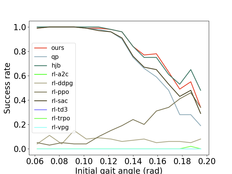
For the bipedal walker experiment, we compare our approach with multiple RL-based approaches (A2C, DDPG, PPO, SAC, TD3, TRPO, VPG) and classic methods (QP, HJB) under different initial gait angles. As shown in Fig. 1, our approach can achieve similar-to-HJB performance, outperforming all the RL-baselines and the QP baseline. The largest improvement (comparing to RL methods) is from the ”small initial angles”. And our gain compared to QP-based methods is mostly from the ”large initial angles”, which might because the large deviation from the target gait angle makes the linearization more inaccurate, hence the QP-based method cannot achieve good performance.
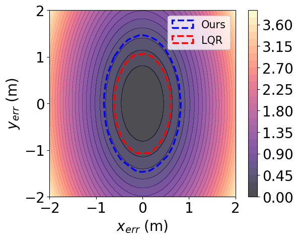
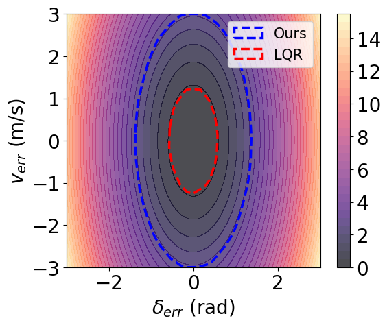
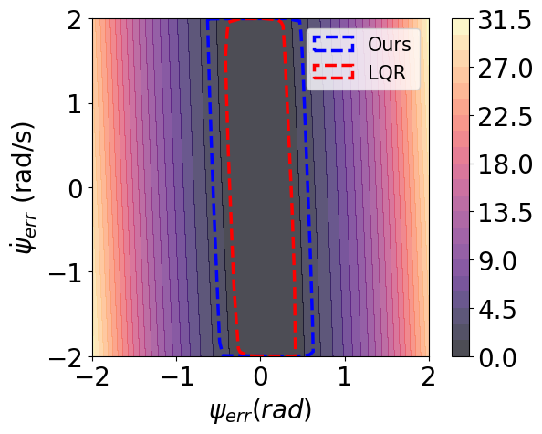
Appendix I Visualization of learned RoA
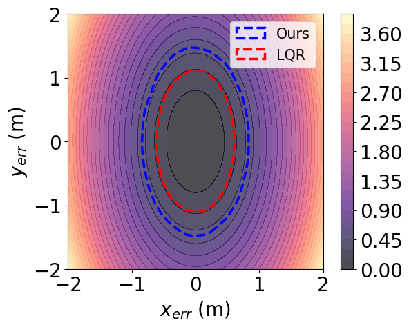
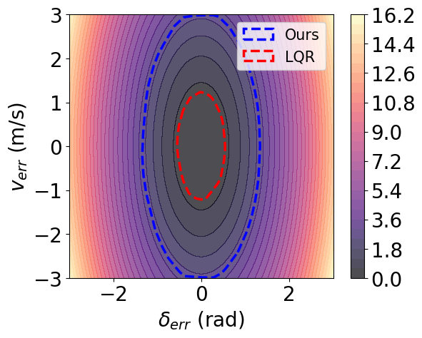
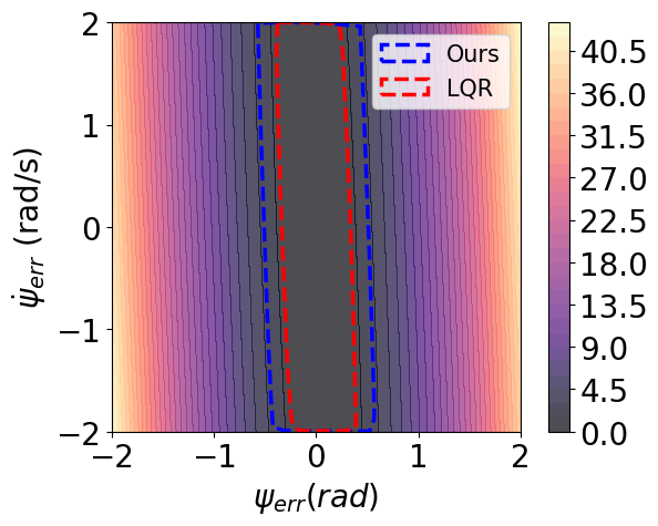
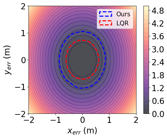
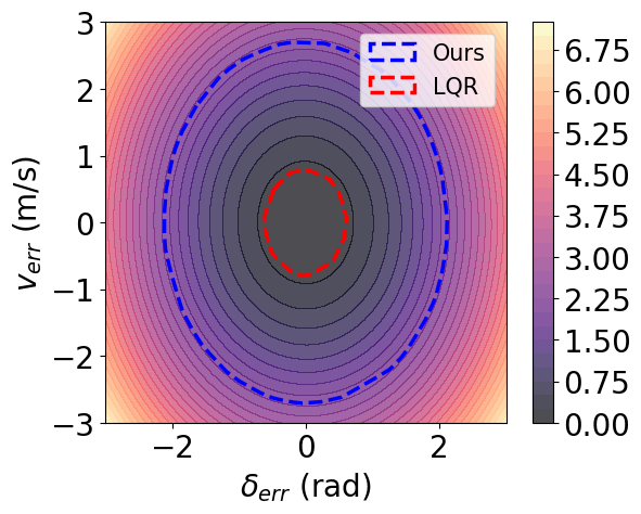
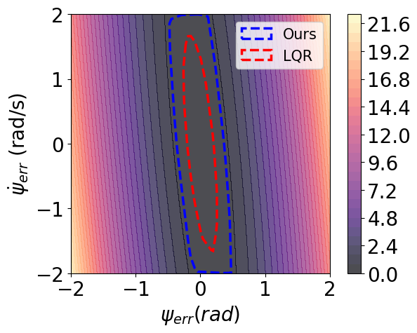
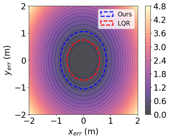
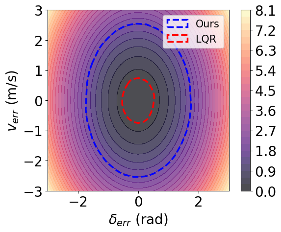
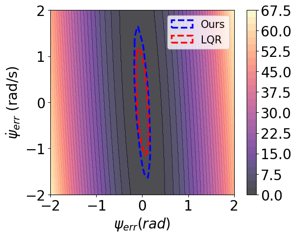
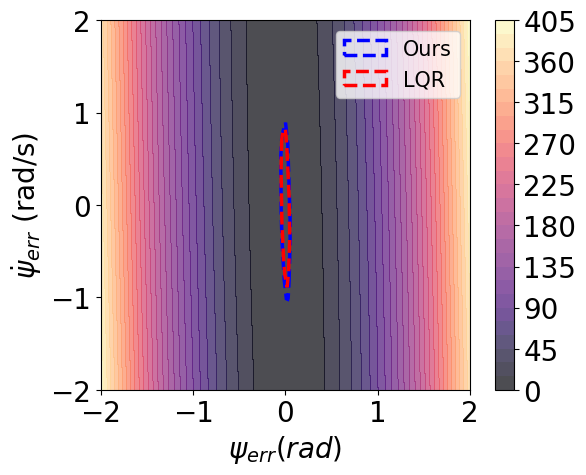
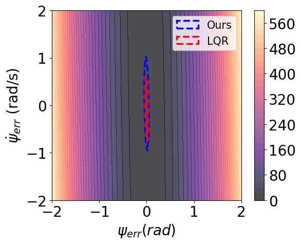
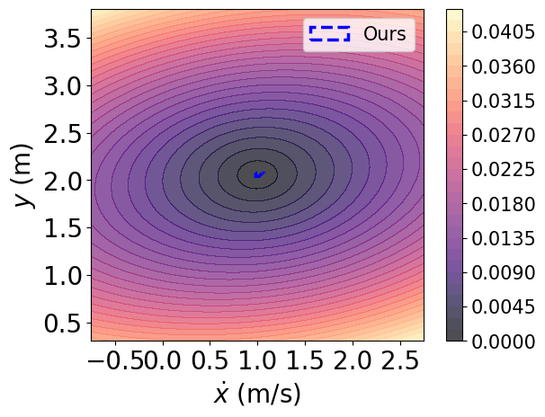
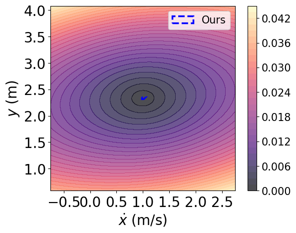
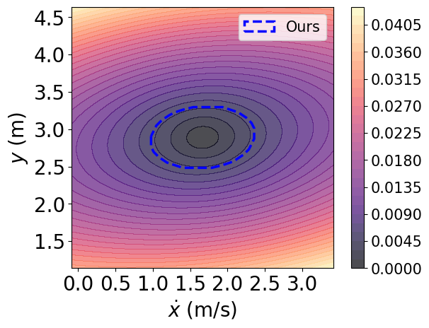
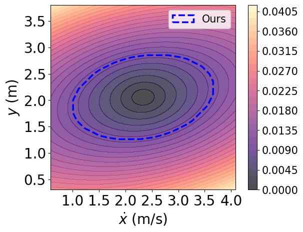
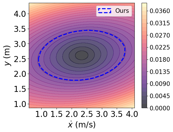
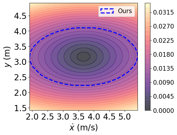
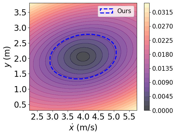
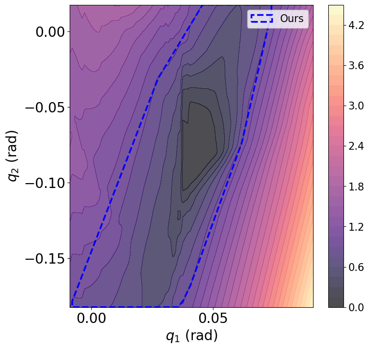
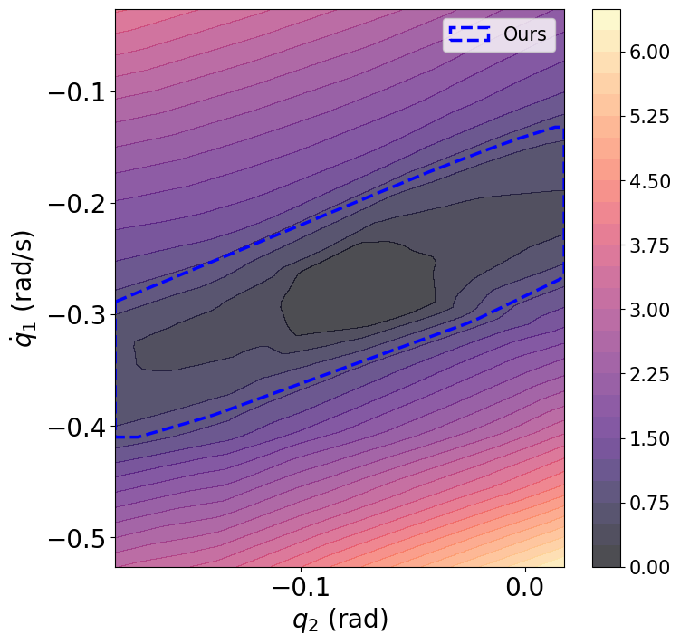
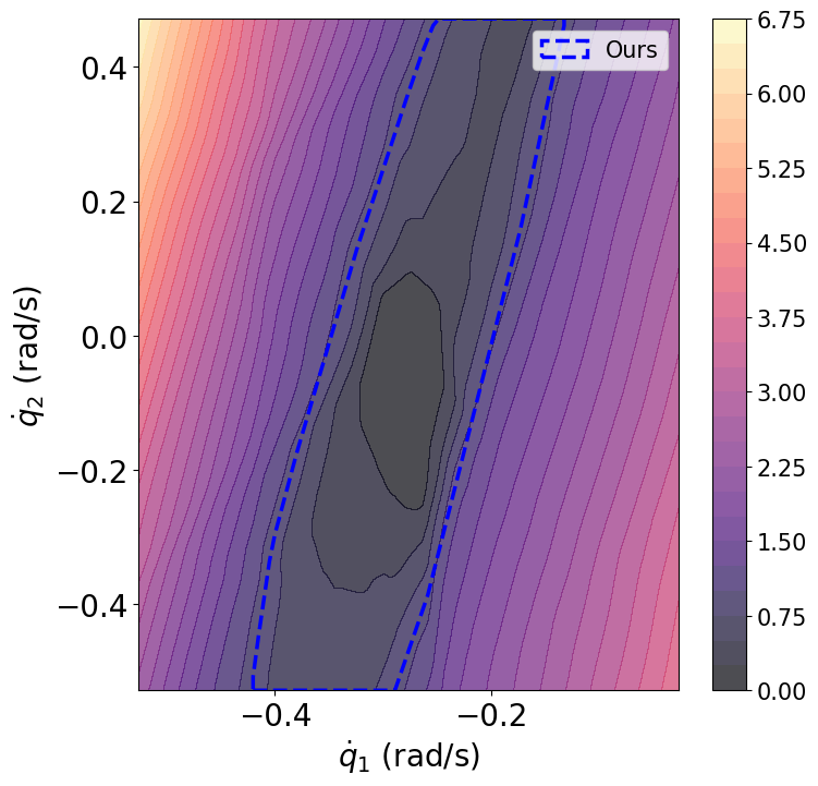
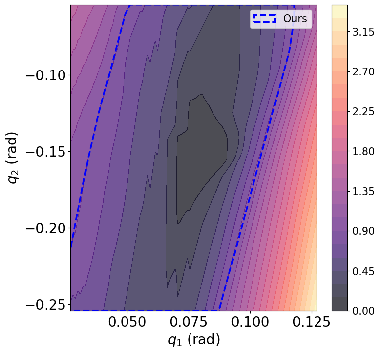
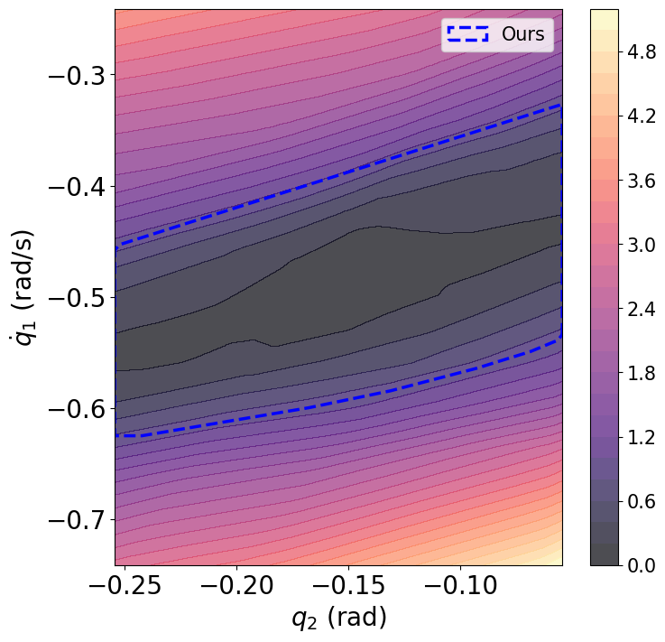
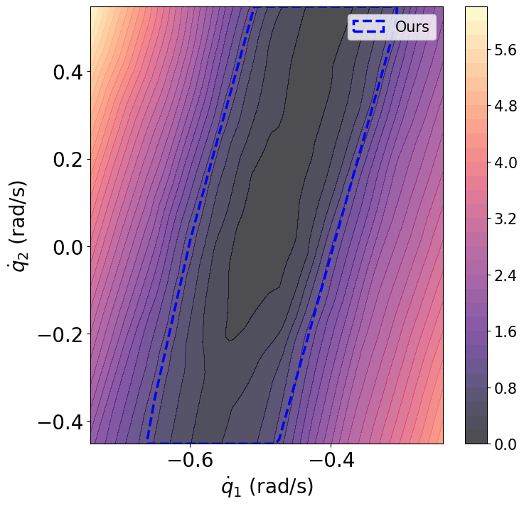
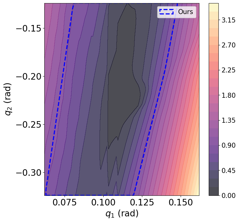
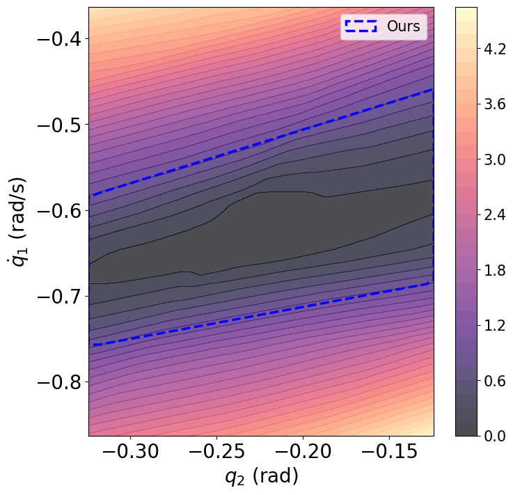
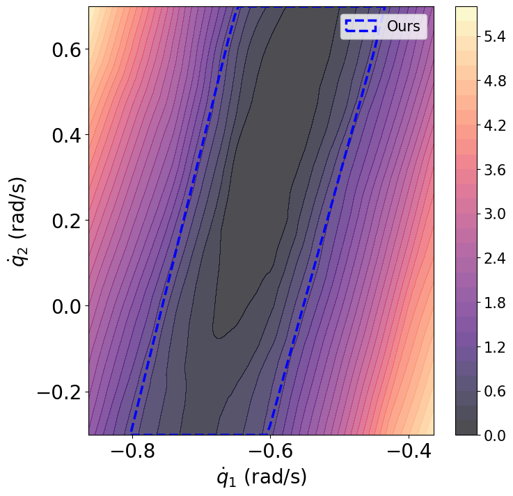
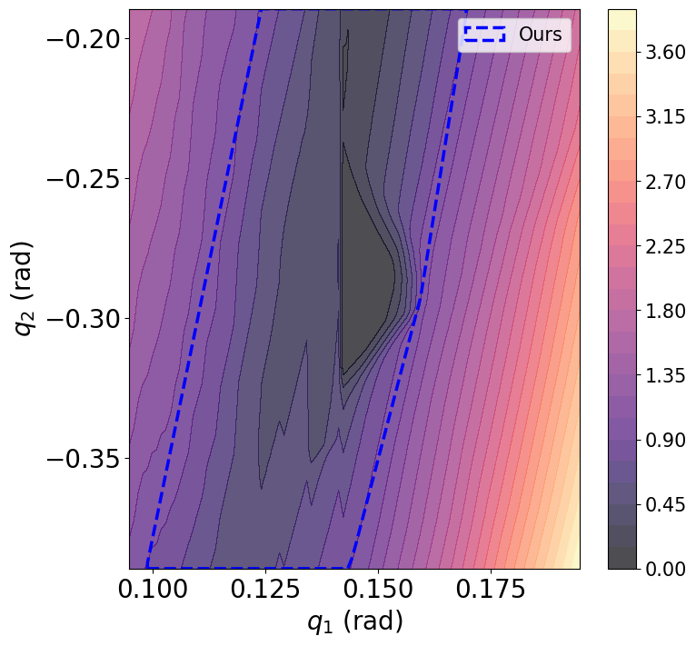
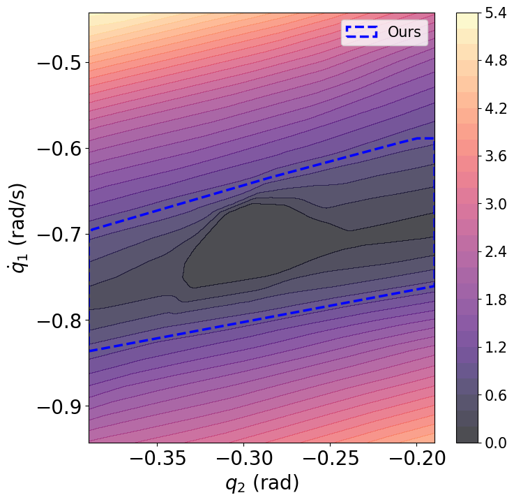
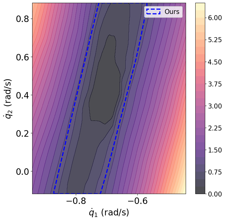
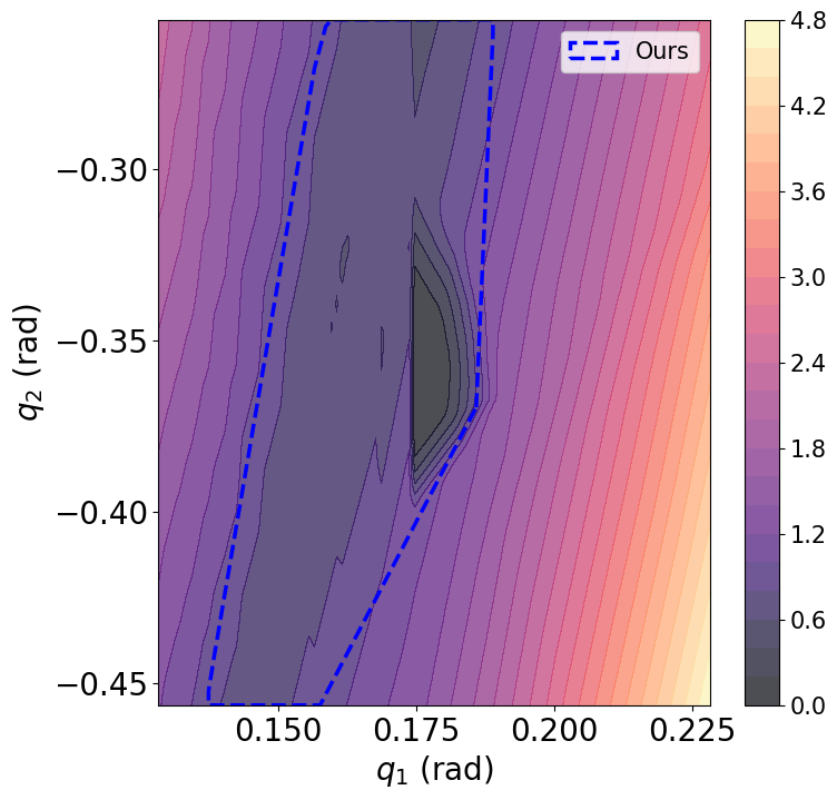
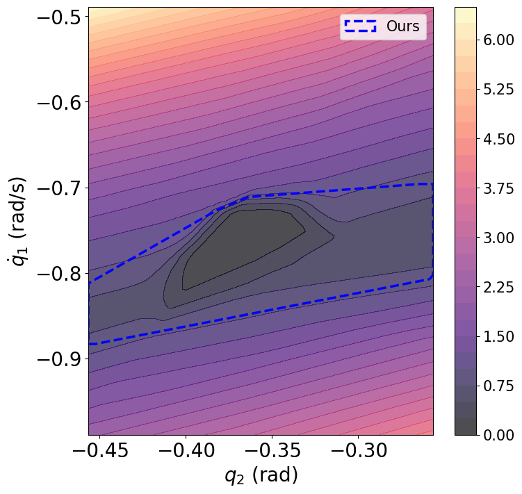
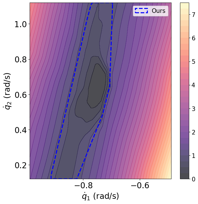
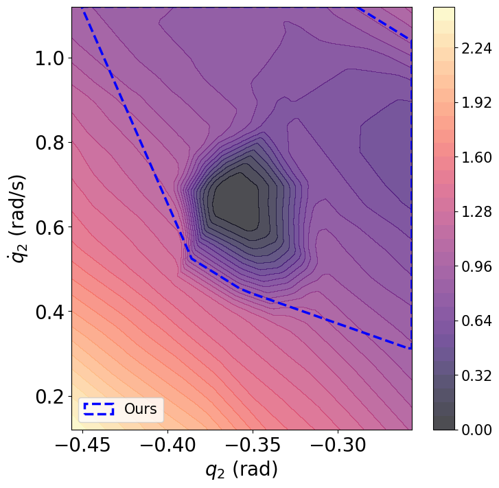
From Fig. LABEL:fig:supple-car-roa-02 to Fig. LABEL:fig:supple-walker-roa-04, we show the visualization of the learned RoA in all three experiments under different configurations.
fig:supple-car-roa-02
\subfigure[- plane]
 \subfigure[- plane]
 \subfigure[- plane]
 \subfigure[- plane]
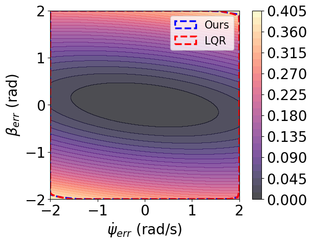
fig:supple-car-roa-03
\subfigure[- plane]
 \subfigure[- plane]
 \subfigure[- plane]
 \subfigure[- plane]
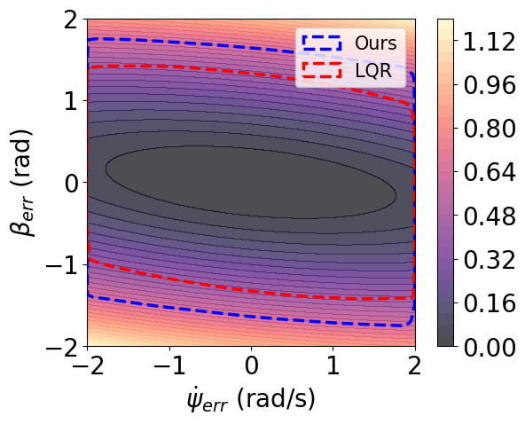
fig:supple-car-roa-04
\subfigure[- plane]
 \subfigure[- plane]
 \subfigure[- plane]
 \subfigure[- plane]
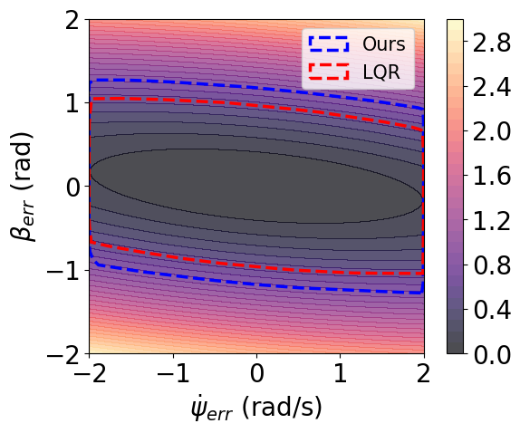
fig:supple-car-roa-05
\subfigure[- plane]
 \subfigure[- plane]
 \subfigure[- plane]
 \subfigure[- plane]
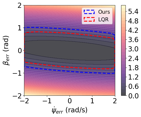
fig:supple-car-roa-08
\subfigure[- plane]
 \subfigure[- plane]
 \subfigure[- plane]
 \subfigure[- plane]
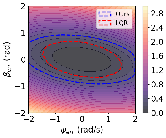
fig:supple-car-roa-09
\subfigure[- plane]
 \subfigure[- plane]
 \subfigure[- plane]
 \subfigure[- plane]
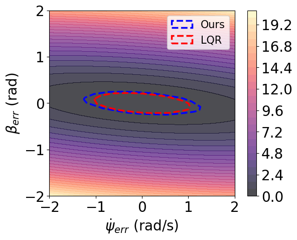
fig:supple-car-roa-12
\subfigure[- plane]
 \subfigure[- plane]
 \subfigure[- plane]
 \subfigure[- plane]
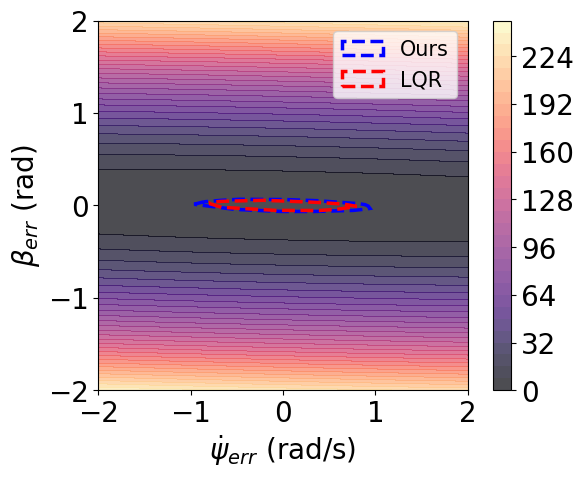
fig:supple-car-roa-13
\subfigure[- plane]
 \subfigure[- plane]
 \subfigure[- plane]
 \subfigure[- plane]
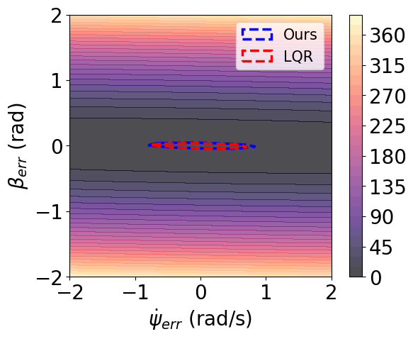
fig:supple-pogo-roa-00
\subfigure[apex velocity=1.0 m/s, apex height= 2.1 m]
 \subfigure[apex velocity=1.0 m/s, apex height= 2.3 m]
 \subfigure[apex velocity=1.0 m/s, apex height= 2.6 m]
 \subfigure[apex velocity=1.0 m/s, apex height= 2.9 m]

fig:supple-pogo-roa-01
\subfigure[apex velocity=1.0 m/s, apex height= 3.2 m]
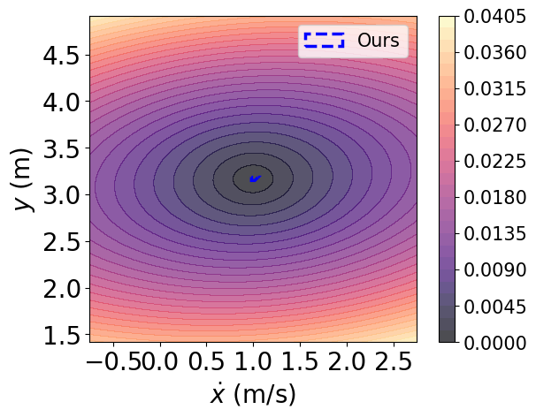 \subfigure[apex velocity=1.3 m/s, apex height= 2.1 m]
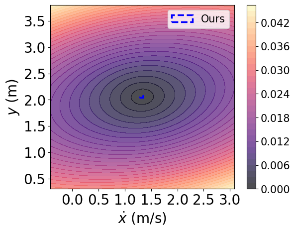 \subfigure[apex velocity=1.3 m/s, apex height= 2.3 m]
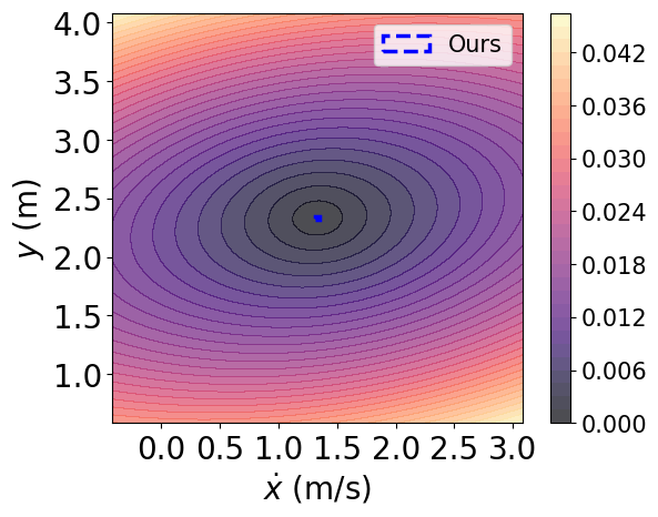 \subfigure[apex velocity=1.3 m/s, apex height= 2.6 m]
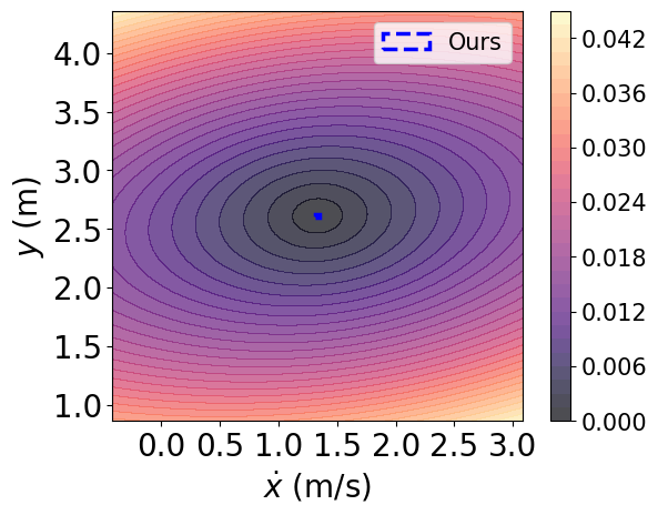
fig:supple-pogo-roa-02
\subfigure[apex velocity=1.3 m/s, apex height= 2.9 m]
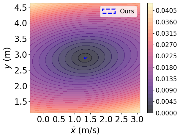 \subfigure[apex velocity=1.3 m/s, apex height= 3.2 m]
 \subfigure[apex velocity=1.7 m/s, apex height= 2.1 m]
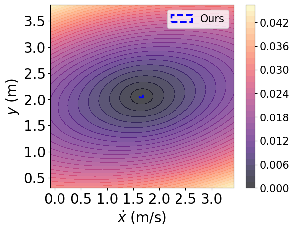 \subfigure[apex velocity=1.7 m/s, apex height= 2.3 m]
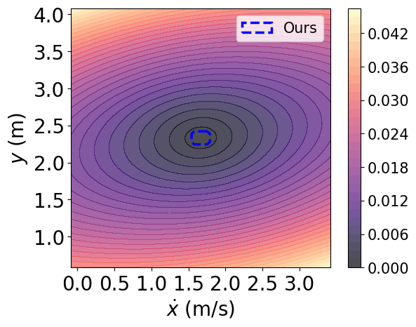
fig:supple-pogo-roa-03
\subfigure[apex velocity=1.7 m/s, apex height= 2.6 m]
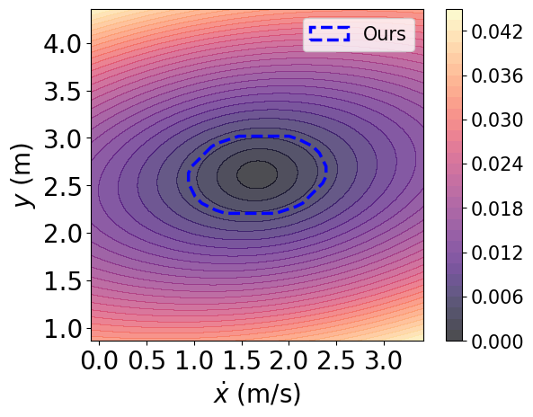 \subfigure[apex velocity=1.7 m/s, apex height= 2.9 m]
 \subfigure[apex velocity=1.7 m/s, apex height= 3.2 m]
 \subfigure[apex velocity=2.0 m/s, apex height= 2.1 m]
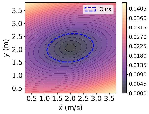
fig:supple-pogo-roa-04
\subfigure[apex velocity=2.0 m/s, apex height= 2.3 m]
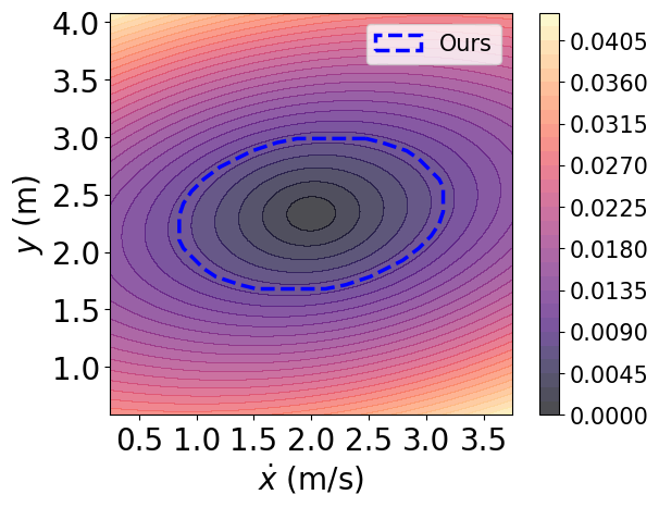 \subfigure[apex velocity=2.0 m/s, apex height= 2.6 m]
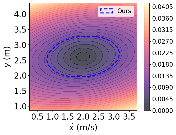 \subfigure[apex velocity=2.0 m/s, apex height= 2.9 m]
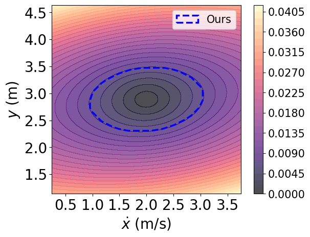 \subfigure[apex velocity=2.0 m/s, apex height= 3.2 m]
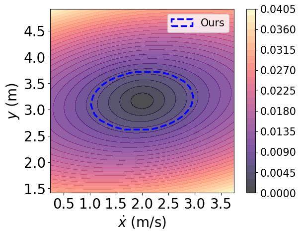
fig:supple-pogo-roa-05
\subfigure[apex velocity=2.3 m/s, apex height= 2.1 m]
 \subfigure[apex velocity=2.3 m/s, apex height= 2.3 m]
 \subfigure[apex velocity=2.3 m/s, apex height= 2.6 m]
 \subfigure[apex velocity=2.3 m/s, apex height= 2.9 m]
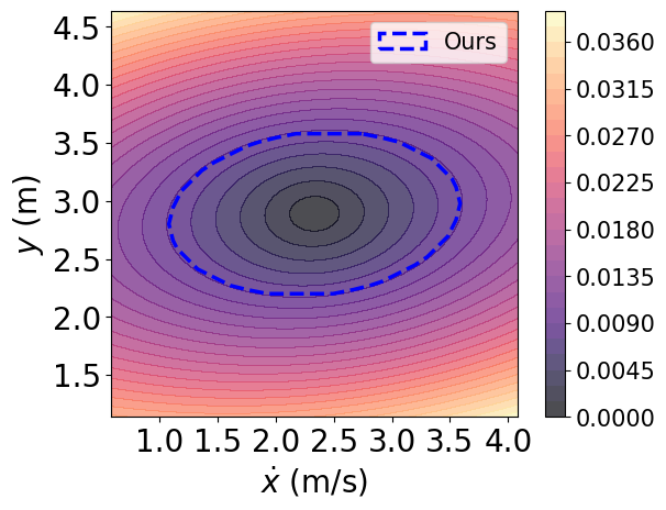
fig:supple-pogo-roa-06
\subfigure[apex velocity=2.3 m/s, apex height= 3.2 m]
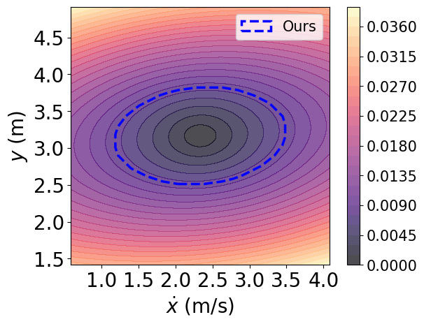 \subfigure[apex velocity=2.7 m/s, apex height= 2.1 m]
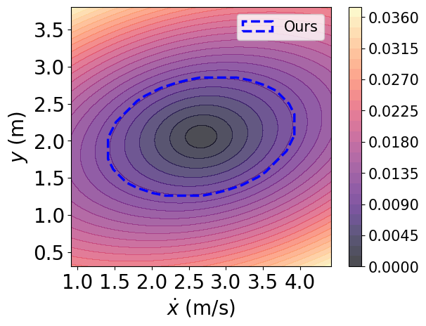 \subfigure[apex velocity=2.7 m/s, apex height= 2.3 m]
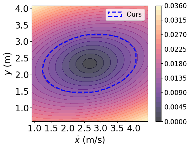 \subfigure[apex velocity=2.7 m/s, apex height= 2.6 m]
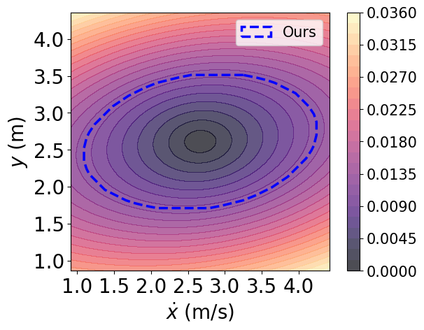
fig:supple-pogo-roa-07
\subfigure[apex velocity=2.7 m/s, apex height= 2.9 m]
 \subfigure[apex velocity=2.7 m/s, apex height= 3.2 m]
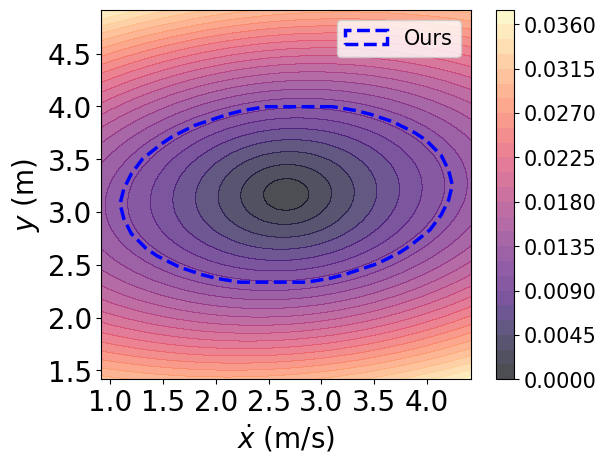 \subfigure[apex velocity=3.0 m/s, apex height= 2.1 m]
 \subfigure[apex velocity=3.0 m/s, apex height= 2.3 m]
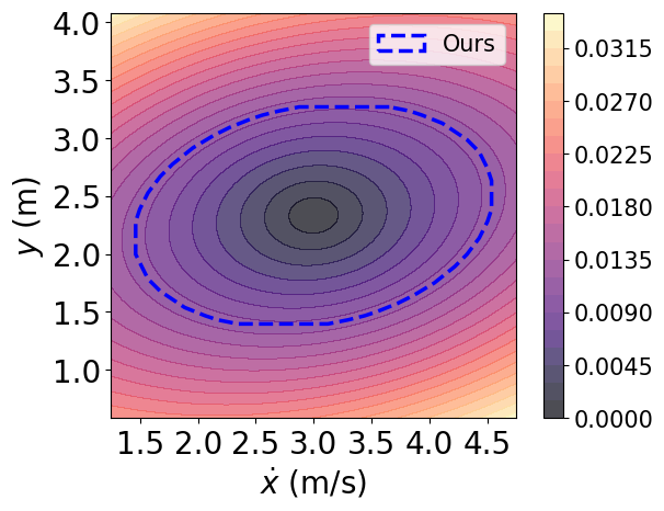
fig:supple-pogo-roa-08
\subfigure[apex velocity=3.0 m/s, apex height= 2.6 m]
 \subfigure[apex velocity=3.0 m/s, apex height= 2.9 m]
 \subfigure[apex velocity=3.0 m/s, apex height= 3.2 m]
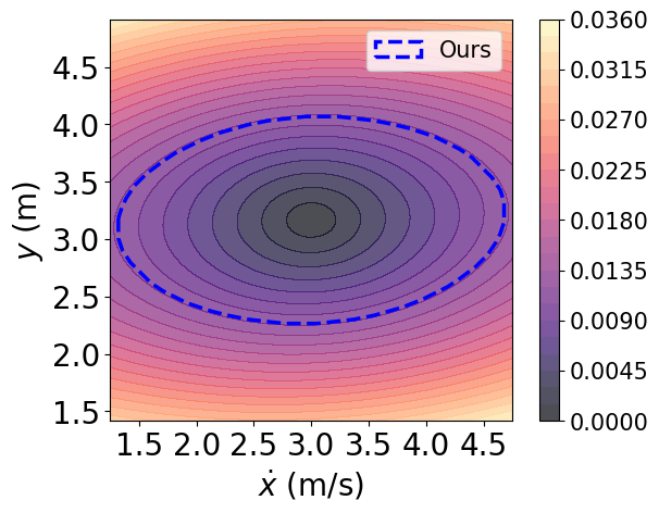 \subfigure[apex velocity=3.3 m/s, apex height= 2.1 m]

fig:supple-pogo-roa-09
\subfigure[apex velocity=3.3 m/s, apex height= 2.3 m]
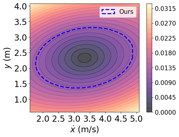 \subfigure[apex velocity=3.3 m/s, apex height= 2.6 m]
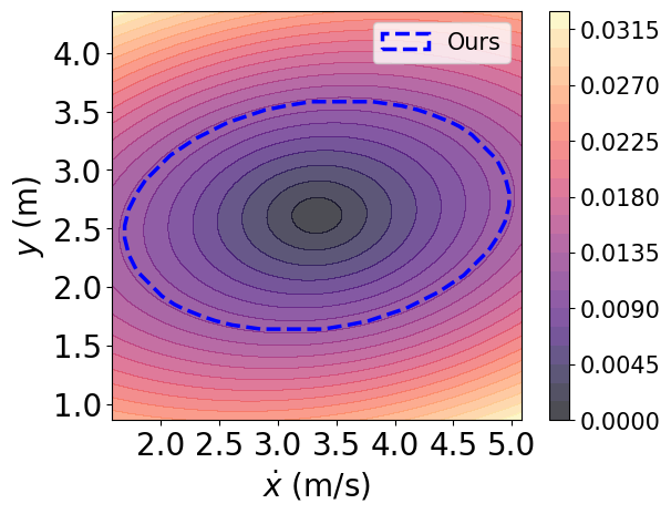 \subfigure[apex velocity=3.3 m/s, apex height= 2.9 m]
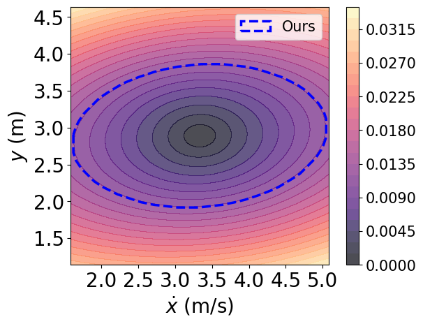 \subfigure[apex velocity=3.3 m/s, apex height= 3.2 m]
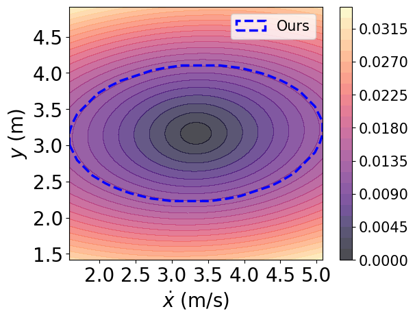
fig:supple-pogo-roa-10
\subfigure[apex velocity=3.7 m/s, apex height= 2.1 m]
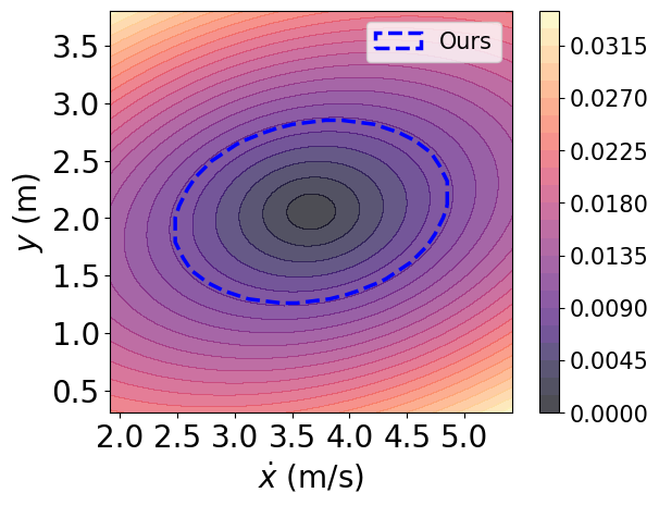 \subfigure[apex velocity=3.7 m/s, apex height= 2.3 m]
 \subfigure[apex velocity=3.7 m/s, apex height= 2.6 m]
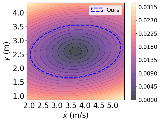 \subfigure[apex velocity=3.7 m/s, apex height= 2.9 m]
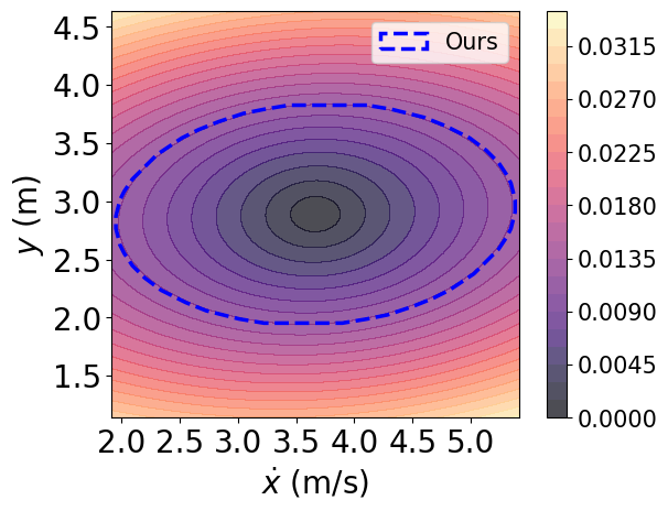
fig:supple-pogo-roa-11
\subfigure[apex velocity=3.7 m/s, apex height= 3.2 m]
 \subfigure[apex velocity=4.0 m/s, apex height= 2.1 m]
 \subfigure[apex velocity=4.0 m/s, apex height= 2.3 m]
 \subfigure[apex velocity=4.0 m/s, apex height= 2.6 m]

fig:supple-walker-roa-00
\subfigure[- plane]
 \subfigure[- plane]
 \subfigure[- plane]
 \subfigure[- plane]
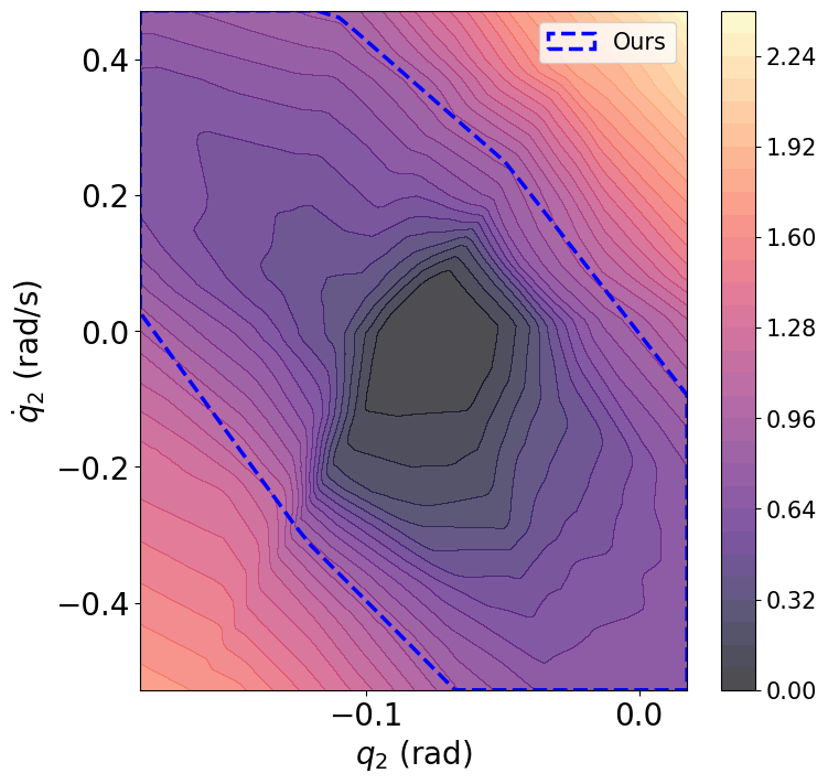
fig:supple-walker-roa-01
\subfigure[- plane]
 \subfigure[- plane]
 \subfigure[- plane]
 \subfigure[- plane]
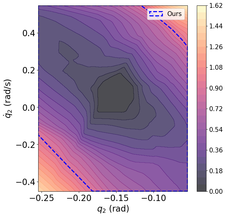
fig:supple-walker-roa-02
\subfigure[- plane]
 \subfigure[- plane]
 \subfigure[- plane]
 \subfigure[- plane]
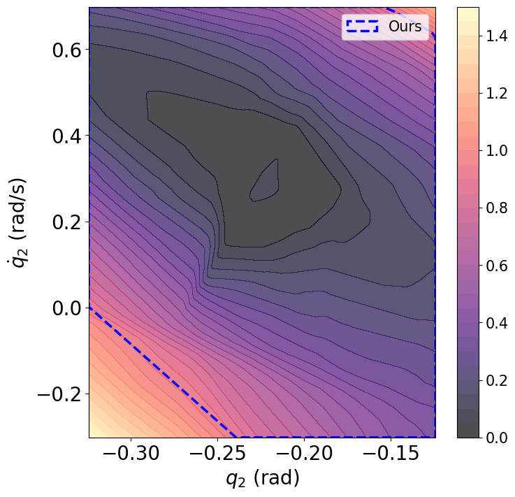
fig:supple-walker-roa-03
\subfigure[- plane]
 \subfigure[- plane]
 \subfigure[- plane]
 \subfigure[- plane]
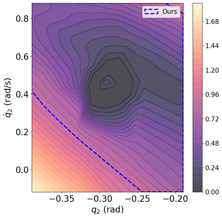
fig:supple-walker-roa-04
\subfigure[- plane]
 \subfigure[- plane]
 \subfigure[- plane]
 \subfigure[- plane]
Appendix J Visualization for the simulations
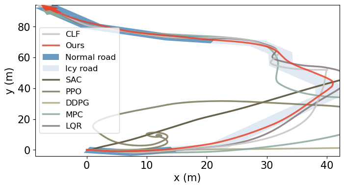
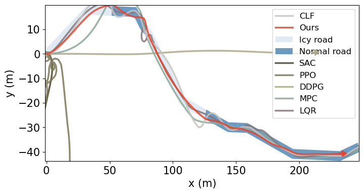
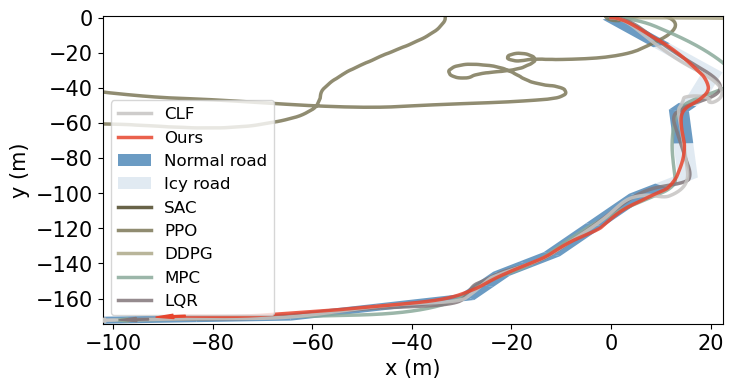
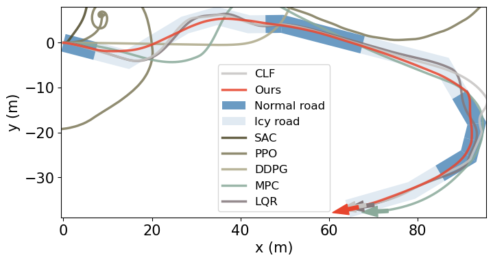
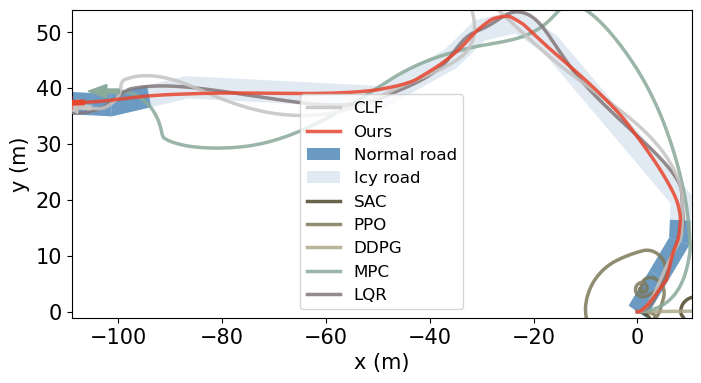
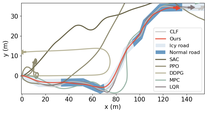
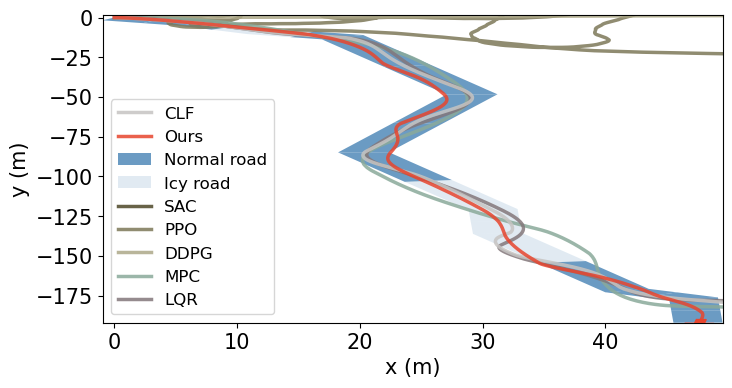
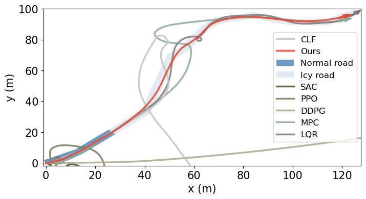
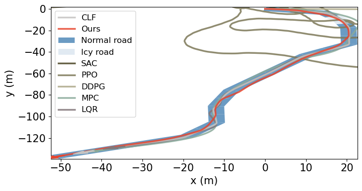
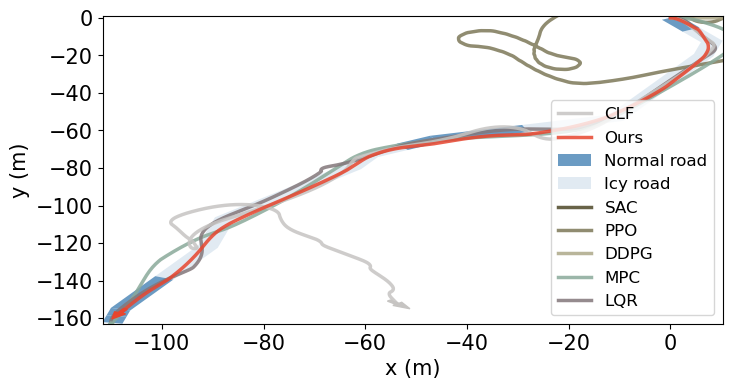
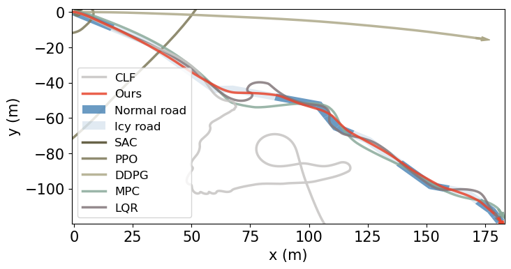
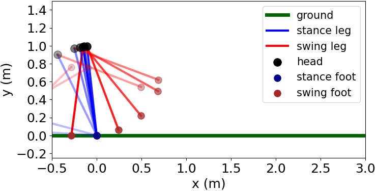
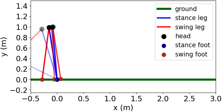
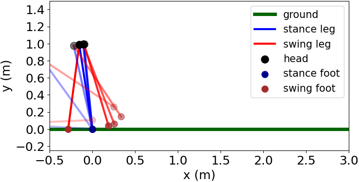
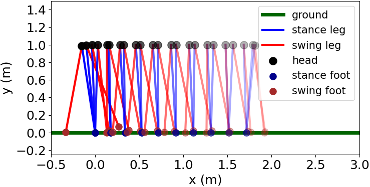
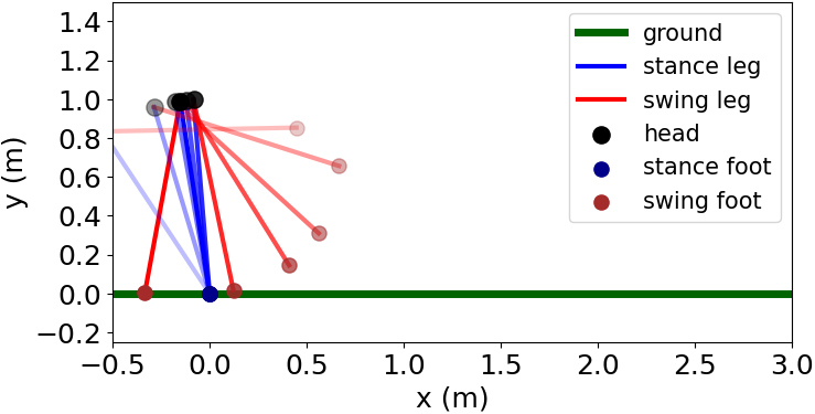
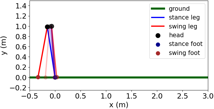
From Fig. LABEL:fig:supple-car-sim-04 to Fig. LABEL:fig:supple-cgw-simx-430, we visualize simulation results for all three experiments under different configurations.
fig:supple-car-sim-04
\subfigure[Trial 00]
 \subfigure[Trial 01]
 \subfigure[Trial 02]
 \subfigure[Trial 03]
 \subfigure[Trial 04]
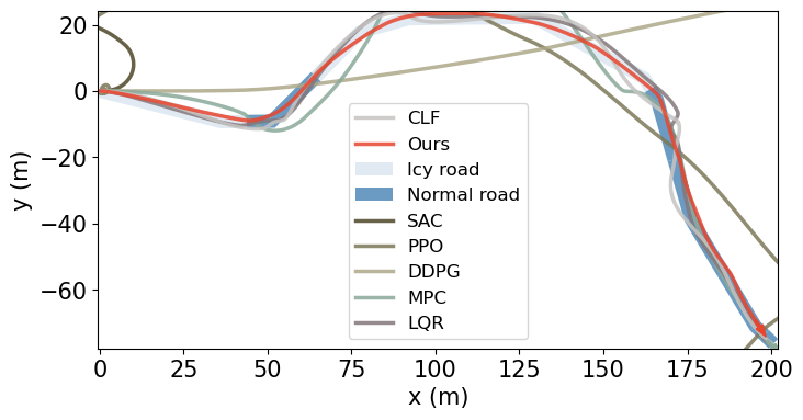
fig:supple-car-sim-09
\subfigure[Trial 05]
 \subfigure[Trial 06]
 \subfigure[Trial 07]
 \subfigure[Trial 08]
 \subfigure[Trial 09]
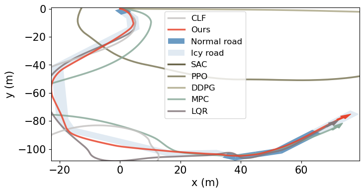
fig:supple-car-sim-14
\subfigure[Trial 10]
 \subfigure[Trial 11]
 \subfigure[Trial 12]
 \subfigure[Trial 13]
 \subfigure[Trial 14]
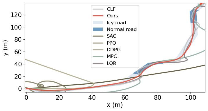
fig:supple-car-sim-19
\subfigure[Trial 15]
 \subfigure[Trial 16]
 \subfigure[Trial 17]
 \subfigure[Trial 18]
 \subfigure[Trial 19]
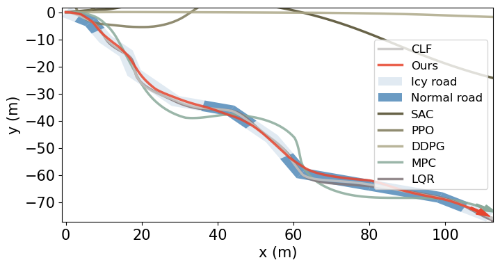
fig:supple-car-sim-24
\subfigure[Trial 20]
 \subfigure[Trial 21]
 \subfigure[Trial 22]
 \subfigure[Trial 23]
 \subfigure[Trial 24]
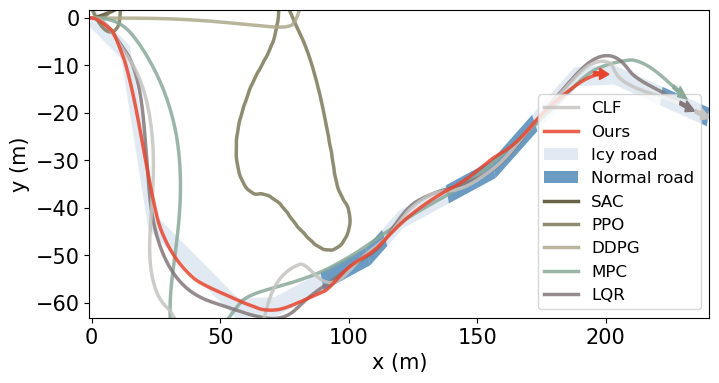
fig:supple-pogo-sim-04
\subfigure[RL-SAC]
 \subfigure[RL-PPO]
 \subfigure[RL-DDPG]
 \subfigure[MPC]
 \subfigure[Ours]

fig:supple-pogo-sim-05
\subfigure[RL-SAC]
 \subfigure[RL-PPO]
 \subfigure[RL-DDPG]
 \subfigure[MPC]
 \subfigure[Ours]

fig:supple-pogo-sim-06
\subfigure[RL-SAC]
 \subfigure[RL-PPO]
 \subfigure[RL-DDPG]
 \subfigure[MPC]
 \subfigure[Ours]
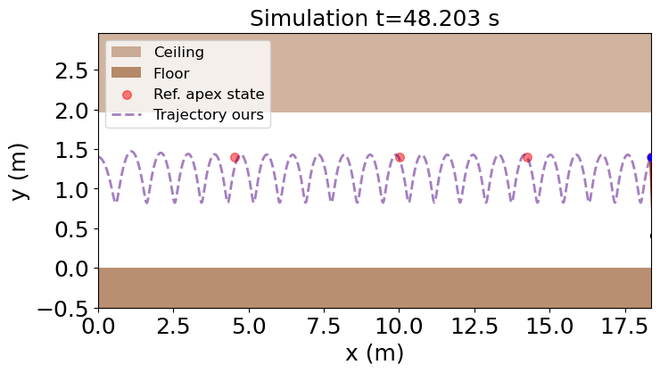
fig:supple-pogo-sim-07
\subfigure[RL-SAC]
 \subfigure[RL-PPO]
 \subfigure[RL-DDPG]
 \subfigure[MPC]
 \subfigure[Ours]
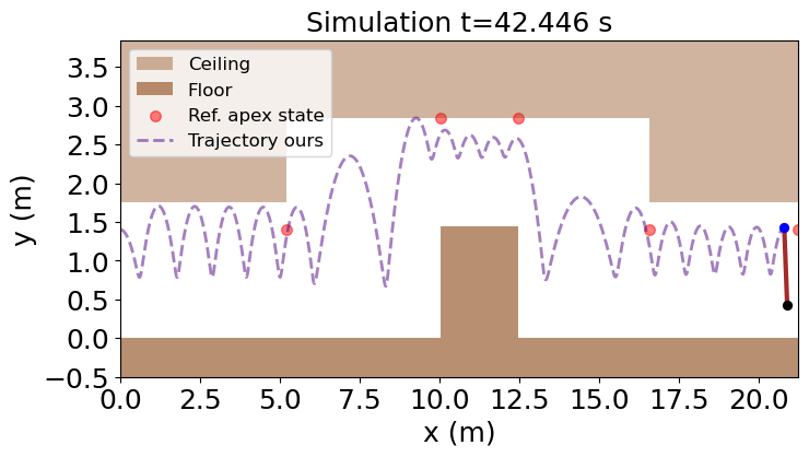
fig:supple-pogo-sim-08
\subfigure[RL-SAC]
 \subfigure[RL-PPO]
 \subfigure[RL-DDPG]
 \subfigure[MPC]
 \subfigure[Ours]
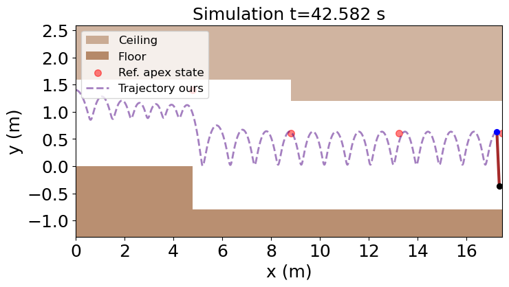
fig:supple-pogo-sim-09
\subfigure[RL-SAC]
 \subfigure[RL-PPO]
 \subfigure[RL-DDPG]
 \subfigure[MPC]
 \subfigure[Ours]
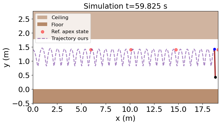
fig:supple-pogo-sim-10
\subfigure[RL-SAC]
 \subfigure[RL-PPO]
 \subfigure[RL-DDPG]
 \subfigure[MPC]
 \subfigure[Ours]
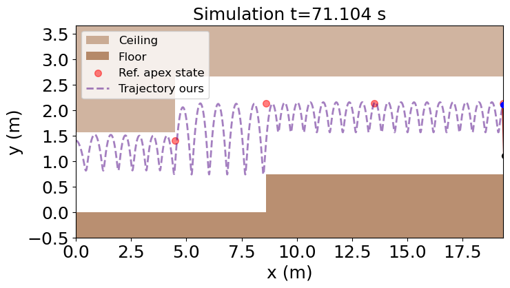
fig:supple-pogo-sim-11
\subfigure[RL-SAC]
 \subfigure[RL-PPO]
 \subfigure[RL-DDPG]
 \subfigure[MPC]
 \subfigure[Ours]
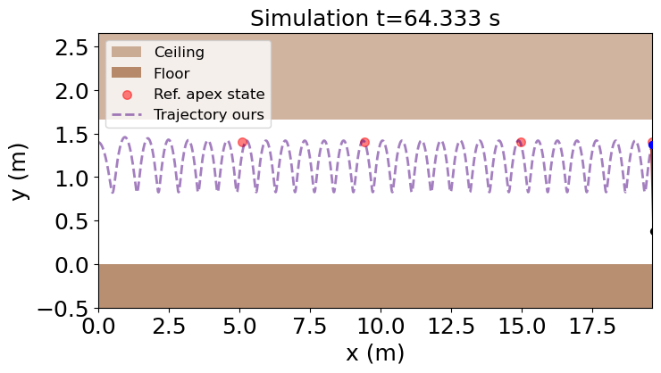
fig:supple-pogo-sim-12
\subfigure[RL-SAC]
 \subfigure[RL-PPO]
 \subfigure[RL-DDPG]
 \subfigure[MPC]
 \subfigure[Ours]
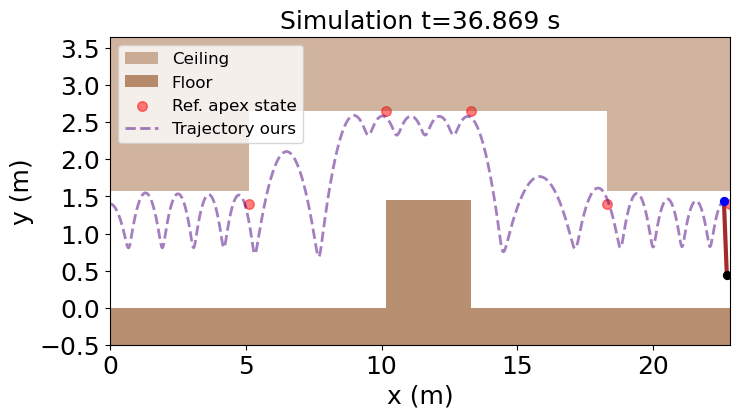
fig:supple-pogo-sim-13
\subfigure[RL-SAC]
 \subfigure[RL-PPO]
 \subfigure[RL-DDPG]
 \subfigure[MPC]
 \subfigure[Ours]
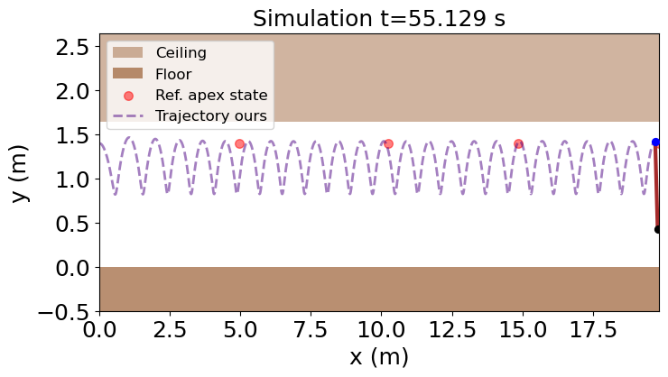
fig:supple-pogo-sim-14
\subfigure[RL-SAC]
 \subfigure[RL-PPO]
 \subfigure[RL-DDPG]
 \subfigure[MPC]
 \subfigure[Ours]

fig:supple-pogo-sim-15
\subfigure[RL-SAC]
 \subfigure[RL-PPO]
 \subfigure[RL-DDPG]
 \subfigure[MPC]
 \subfigure[Ours]
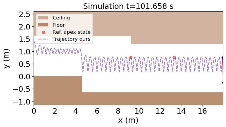
fig:supple-pogo-sim-16
\subfigure[RL-SAC]
 \subfigure[RL-PPO]
 \subfigure[RL-DDPG]
 \subfigure[MPC]
 \subfigure[Ours]
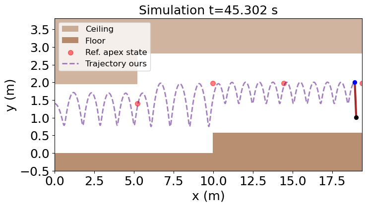
fig:supple-pogo-sim-17
\subfigure[RL-SAC]
 \subfigure[RL-PPO]
 \subfigure[RL-DDPG]
 \subfigure[MPC]
 \subfigure[Ours]
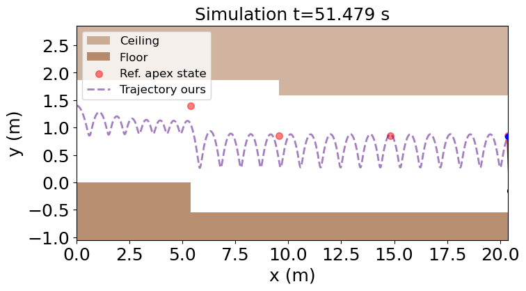
fig:supple-pogo-sim-18
\subfigure[RL-SAC]
 \subfigure[RL-PPO]
 \subfigure[RL-DDPG]
 \subfigure[MPC]
 \subfigure[Ours]
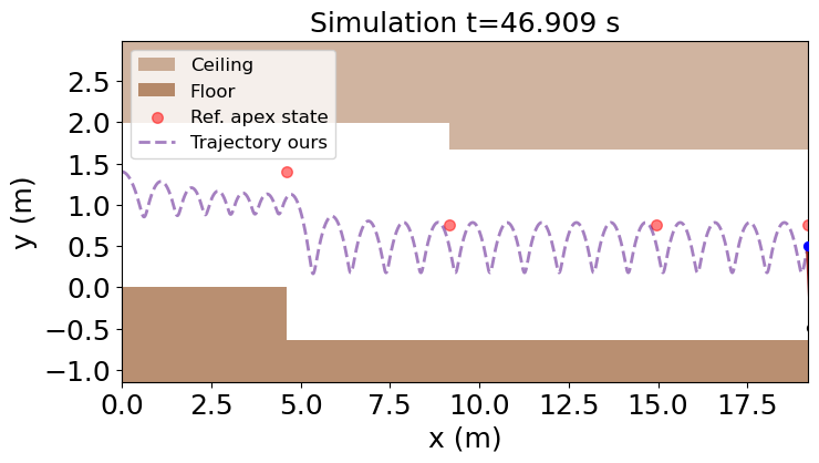
fig:supple-pogo-sim-19
\subfigure[RL-SAC]
 \subfigure[RL-PPO]
 \subfigure[RL-DDPG]
 \subfigure[MPC]
 \subfigure[Ours]
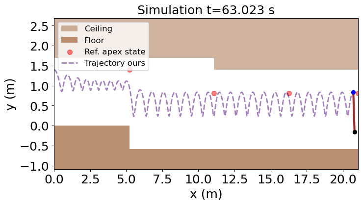
fig:supple-pogo-sim-20
\subfigure[RL-SAC]
 \subfigure[RL-PPO]
 \subfigure[RL-DDPG]
 \subfigure[MPC]
 \subfigure[Ours]
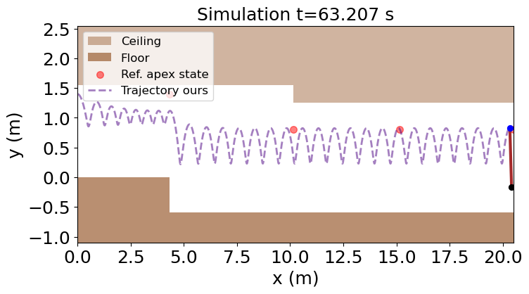
fig:supple-pogo-sim-21
\subfigure[RL-SAC]
 \subfigure[RL-PPO]
 \subfigure[RL-DDPG]
 \subfigure[MPC]
 \subfigure[Ours]
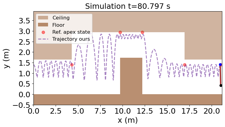
fig:supple-pogo-sim-22
\subfigure[RL-SAC]
 \subfigure[RL-PPO]
 \subfigure[RL-DDPG]
 \subfigure[MPC]
 \subfigure[Ours]
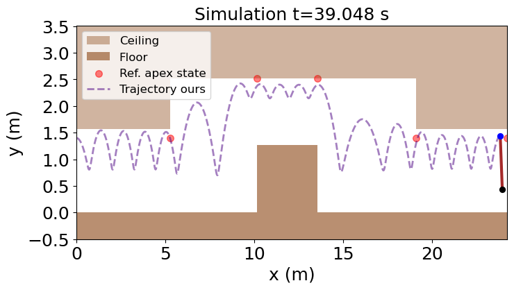
fig:supple-pogo-sim-23
\subfigure[RL-SAC]
 \subfigure[RL-PPO]
 \subfigure[RL-DDPG]
 \subfigure[MPC]
 \subfigure[Ours]
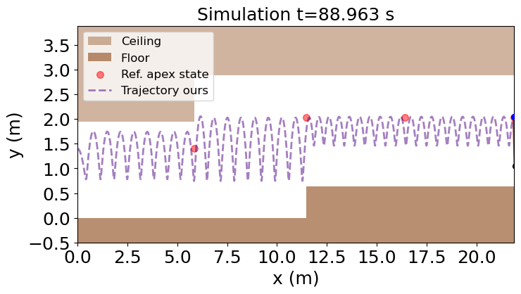
fig:supple-pogo-sim-24
\subfigure[RL-SAC]
 \subfigure[RL-PPO]
 \subfigure[RL-DDPG]
 \subfigure[MPC]
 \subfigure[Ours]
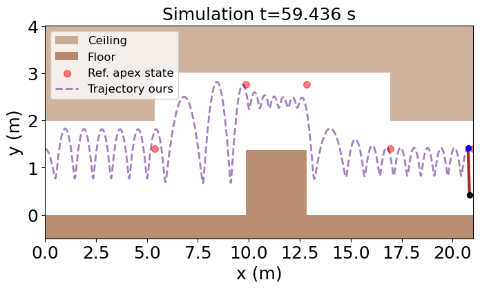
fig:supple-pogo-sim-25
\subfigure[RL-SAC]
 \subfigure[RL-PPO]
 \subfigure[RL-DDPG]
 \subfigure[MPC]
 \subfigure[Ours]
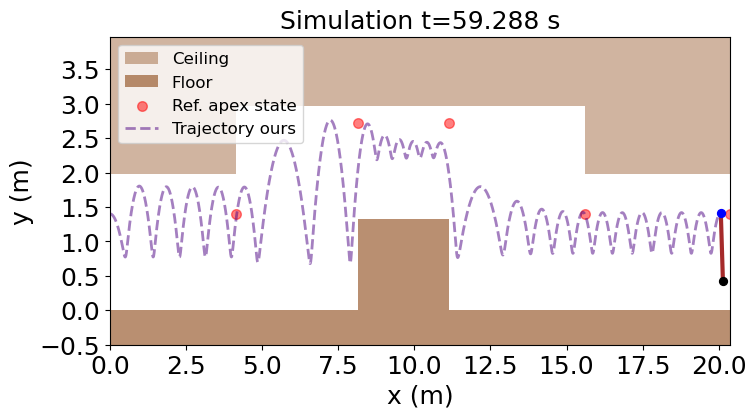
fig:supple-pogo-sim-26
\subfigure[RL-SAC]
 \subfigure[RL-PPO]
 \subfigure[RL-DDPG]
 \subfigure[MPC]
 \subfigure[Ours]
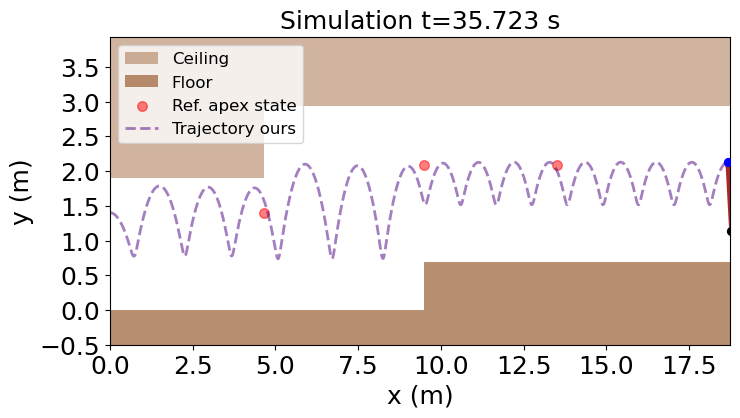
fig:supple-pogo-sim-27
\subfigure[RL-SAC]
 \subfigure[RL-PPO]
 \subfigure[RL-DDPG]
 \subfigure[MPC]
 \subfigure[Ours]
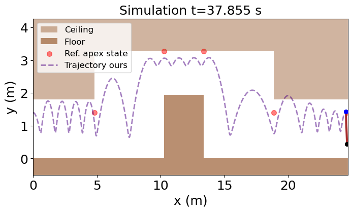
fig:supple-pogo-sim-28
\subfigure[RL-SAC]
 \subfigure[RL-PPO]
 \subfigure[RL-DDPG]
 \subfigure[MPC]
 \subfigure[Ours]
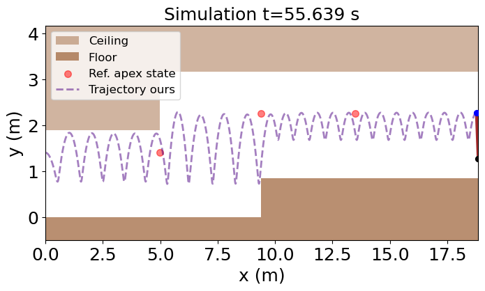
fig:supple-cgw-sim-50
\subfigure[RL-SAC]
 \subfigure[RL-PPO]
 \subfigure[RL-DDPG]
 \subfigure[MPC]
 \subfigure[QP]
 \subfigure[HJB]
 \subfigure[Ours]
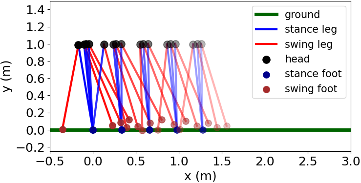
fig:supple-cgw-sim-80
\subfigure[RL-SAC]
 \subfigure[RL-PPO]
 \subfigure[RL-DDPG]
 \subfigure[MPC]
 \subfigure[QP]
 \subfigure[HJB]
 \subfigure[Ours]
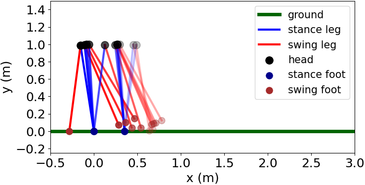
fig:supple-cgw-simx-100
\subfigure[RL-SAC]
 \subfigure[RL-PPO]
 \subfigure[RL-DDPG]
 \subfigure[MPC]
 \subfigure[QP]
 \subfigure[Ours]
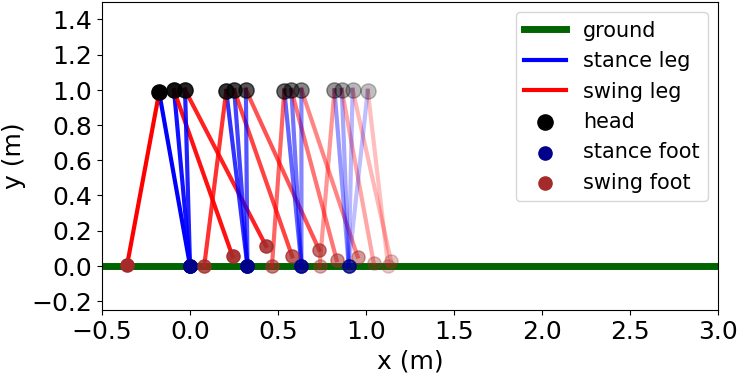
fig:supple-cgw-simx-130
\subfigure[RL-SAC]
 \subfigure[RL-PPO]
 \subfigure[RL-DDPG]
 \subfigure[MPC]
 \subfigure[QP]
 \subfigure[Ours]
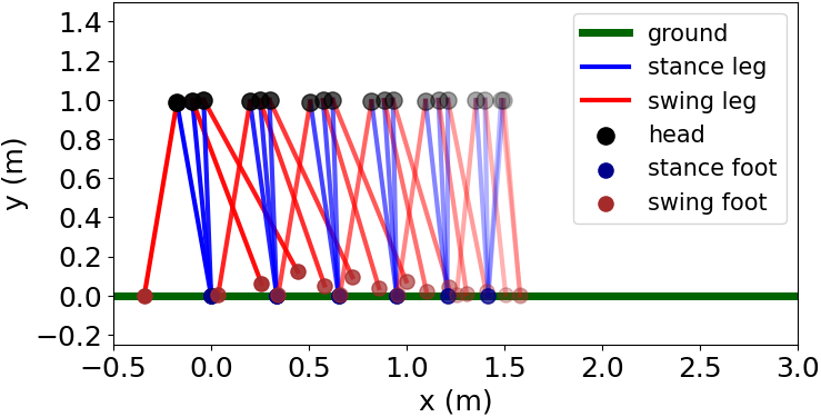
fig:supple-cgw-simx-260
\subfigure[RL-SAC]
 \subfigure[RL-PPO]
 \subfigure[RL-DDPG]
 \subfigure[MPC]
 \subfigure[QP]
 \subfigure[Ours]
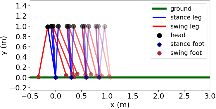
fig:supple-cgw-simx-430
\subfigure[RL-SAC]
 \subfigure[RL-PPO]
 \subfigure[RL-DDPG]
 \subfigure[MPC]
 \subfigure[QP]
 \subfigure[Ours]
