Play to Earn in the Metaverse with Mobile Edge Computing over Wireless Networks: A Deep Reinforcement Learning Approach

Abstract

The Metaverse play-to-earn games have been gaining popularity as they enable players to earn in-game tokens which can be translated to real-world profits. With the advancements in augmented reality (AR) technologies, users can play AR games in the Metaverse. However, these high-resolution games are compute-intensive, and in-game graphical scenes need to be offloaded from mobile devices to an edge server for computation. In this work, we consider an optimization problem where the Metaverse Service Provider (MSP)’s objective is to reduce downlink transmission latency of in-game graphics, the latency of uplink data transmission, and the worst-case (greatest) battery charge expenditure of user equipments (UEs), while maximizing the worst-case (lowest) UE resolution-influenced in-game earning potential through optimizing the downlink UE-Metaverse Base Station (UE-MBS) assignment and the uplink transmission power selection. The downlink and uplink transmissions are then executed asynchronously. We propose a multi-agent, loss-sharing (MALS) reinforcement learning model to tackle the asynchronous and asymmetric problem. We then compare the MALS model with other baseline models and show its superiority over other methods. Finally, we conduct multi-variable optimization weighting analyses and show the viability of using our proposed MALS algorithm to tackle joint optimization problems.

I Introduction

Background. The emergence of the Metaverse has brought a myriad of opportunities [2], and play-to-earn is one of the most iconic features. Prior to the introduction of the Metaverse, players would typically play games that sit in their isolated virtual worlds. Each game’s virtual world is disconnected from other games’ worlds and in-game tokens can only be used within the isolated game [3]. From an ownership standpoint, users in these traditional games barely have any ownership over their in-game earnings, tokens and characters as they ultimately belong to the game developers and creators. Yet now, the Metaverse allows players to gain ownership over their in-game token earnings and possessions through blockchain contracts [3]. These contracts certify the legitimacy and ownership of in-game items thus enabling their real-world value. One way players can become profitable is by playing the Metaverse games, such as those within virtual worlds Axie Infinity, Decentraland and The Sandbox. Players can earn in-game tokens, gain in-game possessions, and trade them for real-world fiat currencies [3]. In this paper, we will coin the concept of “earning potential” to represent the maximum earning that a player can obtain, expressed by a function of the parameters (in particular, the resolution of the in-game graphics) that the player has. The earning potential will be a part of our problem formulation.

Differences between this Journal and Our ICC Conference Paper [1]. This journal is an extension of the work done in  [1]. In this journal, we considered the worst-case (lowest) earning potential, across users and transmission steps, in our optimization function in the downlink stage. This is in contrast to our ICC conference version, where we considered the sum of earning potential of the users, across transmission steps. Similarly, for the uplink stage, we considered the worst-case (greatest) battery charge expenditure, across users and transmission steps, in our optimization function. This is in contrast to our ICC conference version, where we considered the sum of battery charge expenditure of users across transmission steps. Another notable difference is that we added a multi-variable optimization weighting analysis in this journal to show the viability of using our algorithm to tackle joint optimization problems. Finally, we provide more details pertaining to the rationale of our work and algorithm.

I-A Problem

Compute-intensive Mobile Augmented Reality (MAR). Many play-to-earn games are developed for mobile devices [4] enabling people to play them whenever and wherever possible to earn in-game currency. Compute-intensive Metaverse play-to-earn games such as Polkacity [5] and Reality Clash [6] are attributed to high-resolution in-game graphics, complex in-game interactions, and increasing adoption of Mobile Augmented Reality (MAR). The core of augmented reality (AR) is to overlay physical world scenes with digital elements, creating a highly immersive and interactive visual experience for AR users [2]. Despite rapid development in AR technologies, current mobile computing technologies are struggling to keep up with the increasing demands of AR applications such as play-to-earn games. Yet in the context of AR play-to-earn games, the fluidity of the gaming experience should be highly regarded as it influences the players’ gameplay. One viable way of dealing with the lack of mobile computing power is to offload the computation and rendering of play-to-earn games to an edge computing server [7].

Inefficient edge computing concerns. In the context of the play-to-earn Metaverse games, an in-game graphics offloading example pipeline can be described as such: In a single iteration of transmissions, high-resolution in-game graphics can first be downloaded from the Metaverse Service Provider’s Base Stations (MBSs) to the players, in which players will view in-game scenes and take actions, altering the in-game scenes. For clarity, note that MBSs can be viewed as edge-computing base stations assigned by the Metaverse service provider. These altered in-game scenes are then offloaded back to the MBSs for computation. In the downlink leg, delivery of poor in-game graphic resolution and large downlink latency is often a concern. Take the following scenario as an example - Several MBSs are catering in-game graphic computation services to multiple players; i.e., user equipments (UEs). If there is inefficient allocation of users to MBSs (i.e., too many UEs are allocated to the same MBS or UEs are allocated to MBS situated far away), there will be greater signal interference or lower transmission efficiency, which reduces the overall rate of transmission of in-game graphical data. In such a case, this results in an increase in downlink latency and also overall poor in-game graphical smoothness. In the uplink leg, there is often a concern pertaining to both the latency of uplink transmission and UE device energy usage. Specifically, if the selected power for the uplink transmission is optimal, the effective signal between the UEs and MBS will be improved. This will result in a decrease in uplink transmission latency. Conversely, a poor UE uplink power selection may result in greater signal interference between UEs and MBS, reducing the effective signal between UEs and MBS and hence increasing the latency for uplink transmission. This results in a decrement in in-game earning potential, fluidity, and hours of play.

Formulated Problem. Finding an optimal strategy to maximize the UEs’ play-to-earn profitability, while minimizing device energy consumption and transmission latency is non-trivial. First and foremost, a Metaverse play-to-earn framework will have to account for (i) profitability of players, (ii) fluidity (smoothness) of in-game player experience, and (iv) player device’s battery level and energy consumption, in the interest of player retention. These three factors are key considerations when developing a Metaverse play-to-earn framework. We formulate the problem in a way where the Metaverse Service Provider (MSP) aims to minimize the (i) graphical data latency of downlink transmission delay, (ii) latency of uplink data transmission, (iii) and worst-case (greatest) UE device battery charge expenditure, while maximizing (iv) the players’ worst-case (lowest) in-game earning potential influenced by graphic resolution, by optimizing the UE-MBS allocation, and UE uplink transmit power. This is to ensure player retention by improving their overall in-game fluidity, experience, profitability and UE battery charge for long periods of play. We choose to maximize the worst-case (lowest) profit and minimize the worst-case (greatest) batter charge expenditure across the UEs as our aim is to ensure that no players’ interests are neglected, in hopes of player retention.

I-B Our Approach and Rationale

To tackle these abovementioned problems, we introduce a novel Multi-Agent Loss-Sharing (MALS) reinforcement learning (RL)-based orchestrator which houses a downlink (DL) agent and an uplink (UL) agent that optimizes the UE-MBS allocation and uplink transmission power to maximize the utility function (the aim of the Metaverse Service Provider). Specifically, we designed the DL agent to be a discrete-action space RL agent which chooses the UE-MBS allocation, and a continuous-action space UL agent which selects UE uplink power to maximize the utility function. However, instead of providing the agents with an overarching objective function, the agents are assigned to tackle objectives that are within their control. It is intuitive to have different objectives in each DL and UL stages as the data transmitting party in each stage, and hence, the variables in which they control, differ. This is to avoid “confusing” the agents while providing the agents with more explicit goals. Note that the agents are asymmetric, in that they have separate objectives and action space types. The UL and DL agents are also executed asynchronously. The DL agent will first select the UE-MBS allocation, conduct the DL data transfer, followed by the UL transmission and UL power selection by the UL agent. Although the DL and UL processes seem distinct, asymmetric, and are executed asynchronously, it is important to optimize both stages concurrently.

Reinforcement learning approach over convex optimization. We proposed a complex play-to-earn mobile edge computing problem which is not naturally convex as the UE-MBS allocation is constrained to integer values. By utilizing convex optimization approaches, we can only yield approximate solutions by relaxing the constraints. Secondly, our proposed problem involves the optimization of UE-MBS allocation. The complexity of the allocation problem is large, due to the possible combinations of UE-MBS allocation and the number of transmission iterations (sequential problem). Such high-complexity problems render convex optimization approaches infeasible. Thirdly, we consider the cumulative in-game profit and cumulative UE device energy expenditure in our problem. This renders our problem highly sequential and the objective functions cannot be solved independently at each transmission iteration.

What is Multi-Agent-Loss-Sharing? We proposed a novel Multi-Agent-Loss-Sharing (MALS) reinforcement learning-based algorithm to handle the training of two agents in a mix-cooperative scenario. The MALS algorithm builds on the actor-critic (AC) based reinforcement learning algorithms. Similar to traditional interacting, independent dual agents (IDA), each agent will have an actor which executes actions independent of information other than the state it receives. In contrast to IDA, each agent under the MALS implementation will share a critic model with multiple heads which takes in inputs from both actors to calculate personalized advantage values for the update of each actor. The critic losses from each head are summed and used to update the critic. The rationale for summing the losses of both critic heads is to facilitate the cooperative training of both agents. This ensures that the training process reduces the critic multi-head losses concurrently, not neglecting either agent’s model improvement.

Why not apply the CTDE framework? Similar to our proposed MALS implementation, traditional Multi-Agent Reinforcement Learning [8] utilizes an actor-critic, Centralized Training and Decentralized Execution (CTDE) framework. The actor of each agent executes independently (decentralized execution). In contrast to MALS, the critic for each agent under the CTDE framework will share a similar model, taking into account all other agents’ actions (centralized training) in each time step. This CTDE framework is unsuitable to tackle our proposed problem as: (1) our proposed problem is asymmetric. The agents in our work have distinct action spaces, where the DL agent selects discrete-valued UE-MBS allocation while the UL agent selects continuous-valued UE uplink transmission power. The underlying model and hence critic are dissimilar, rendering CTDE an unsuitable method. (2) Our proposed problem is asynchronous. In our proposed scenario, the downlink and uplink agents will alternately execute actions. However, MARL considers all agents’ actions and each agent executes actions simultaneously in each time step. When dealing with asynchronous action executions, each agent’s observation space will only contain the state and action of the other agent. This results in a highly sparse state input, which renders CTDE to be computationally inefficient in tackling our proposed scenario.

Multi-agent sequential dependency. Moreover, the formulation of an asymmetric and asynchronous MEC resource allocation problem causes dependency between agents in the Partially Observation Markov Decision Process (POMDP). In a conventional deterministic, single-agent environment, the environment is only impacted by a single agent’s actions. Hence the environment and rewards perceived by the agent are a result of its own actions. However, in a two-agent, asynchronous execution environment, the environment and rewards perceived by an agent are not solely a consequence of its own actions, but also the action of the other agent. Hence the transition probabilities learnt by an agent are subject to the decisions made by the other agent. Consider the following scenario: An optimal MBS-UE channel allocation in the DL process may result in high data transfer rates from the MBSs to UEs. Consequently, the UEs will receive more data. This may not always be good for such a multi-stage system, as more data received in the DL stage means more data needs to be transmitted in the UL stage. Therefore, the UL stage may face a high data traffic flow, resulting in an overall larger UE power required for the UL transmission. This may result in greater interference due to an overall higher power output by each device. There is strong dependency between an agent facilitating the DL process and the agent facilitating the UL process. Therefore, we have to consider the concurrent orchestration of both UL and DL stages. We seek a new reinforcement learning structure to tackle an asynchronous setting.

Play-to-earn under mobility. The existence of Metaverse games with play-to-earn features on mobile devices would mean that players are expected to be on the move. As players move, their distance from the MBSs changes. This changing distance results in varying channel gain and hence effective rate of data transfer. In our proposed Metaverse play-to-earn framework, we have to take into account players’ (UEs’) mobility.

I-C Existing Literature and Our Contributions

In this subsection, we first present related work and then highlight the contributions of this paper. We divide related studies into different categories: 1) Metaverse communication framework, 2) AR over wireless networks, and 3) deep reinforcement learning for task offloading, where the first two categories are also discussed in our recent conference paper [9].

Metaverse communication framework. Since the Metaverse is still relatively new, limited studies consider Metaverse edge computing problems. In our conference paper [9], we designed a vehicular Metaverse Augmented Reality socialization over 6G wireless networks scenario and devised artificial intelligence techniques to tackle their proposed optimization problem. In another of our conference paper [10], we devised a machine learning approach to tackle an adversarial patch detection in defence of digital twinning over wireless networks problem. The authors of [11] introduced an Internet of Things (IoT)-based digital twinning over wireless networks scenario and proposed a framework to tackle a wireless network resource allocation problem. Ng et al. [12] designed stochastic optimization-based resource allocation to obtain the minimum cost of a Metaverse service provider in the education sector context. Xu et al. [13] presented an incentive mechanism based on machine learning for VR in the Metaverse, using auction theory to obtain the optimal pricing and allocation, and deep reinforcement learning to accelerate the auction process.

AR over wireless networks. Apart from Metaverse-related resource allocation studies, there are several works [14, 15, 16, 17] which have studied resource management or optimization problems concerning virtual, augmented or extended reality over wireless networks. Chen et al. [14] considered a resource allocation problem and devised a distributed machine learning algorithm to tackle it. The authors of [15] studied the optimization of VLC access points (VAP) and user-base station association to empower virtual reality over wireless networks for indoor environments. Liu et al. [16] proposed an MAR over wireless network scenario and utilized convex optimization techniques to solve an object detection for MAR and latency of computation offloading problem. Wang et al. [17] aimed to minimize the energy consumption of users using mobile augmented reality systems by optimizing the MAR configuration as well as the radio resource allocation. In [18], the authors studied optimization problems which consider the Quality of Experience (QoE) of users.

Deep reinforcement learning for task offloading. There are several works utilizing deep reinforcement learning to optimize task offloading [19, 20, 21]. However, these works consider the system as a single entity. In practice, the DL and UL processes may involve different parties in the transmission process and may have different objectives.

In contrast to these abovementioned works, there are several works which consider the concurrent optimization of several variables within their objective function and proposed reinforcement learning approaches to handle them. Guo et al. [22] utilized a Centralized Training and Decentralized Execution (CTDE) framework to tackle handover and power selection. Similarly, He et al. [23] adopted the CTDE [8] framework to address the user to channel allocation and transmission power selection problem. Nevertheless, the abovementioned works are not concerned with a multi-stage, asynchronous transmission scenario, as studied in our paper.

Contributions. We make the following contributions to the field:

• Dual Joint Optimization: We formulate a multi-variable optimization problem for play-to-earn enabled Metaverse with mobile edge computing.

• Multi-Agent-Loss-Sharing: We propose a novel asymmetric and asynchronous multi-agent loss-sharing reinforcement learning-based orchestrator to tackle a novel asynchronous and asymmetric wireless communication problem.

• Comparison of our proposed methods against baseline models: We compare our (i) proposed method MALS with baseline methods such as (ii) independent dual-agent (IDA) and (iii) CTDE [8] reinforcement learning algorithm. The comparison shows the superiority of our proposed method in handling asynchronous executions.

• Analyses of weighted utility objective functions: We provide in-depth analyses of how the different weights on each factor in the joint optimization functions influence reward and other variables. These analyses provide insights into solving multi-agent joint-optimization problems.

We organize the rest of the paper as follows. Section II covers the details of our Metaverse play-to-earn optimization problem while Section III discusses the formulation of the problem in the context of reinforcement learning. Section IV introduces our proposed novel MALS deep reinforcement learning model and discusses the algorithm in detail. In Section V, we carry out thorough experiments to compare different methods to showcase the superiority of the MALS algorithm in handling asymmetric and asynchronous problems. Analyses on the weighting of variables in the joint utility functions are also conducted to demonstrate the feasibility of our proposed approach across various weights of joint-variable optimization problems. Finally, Section VI concludes the paper.

II System Model

Problem Scenario. Consider the real-time downlink (DL) and uplink (UL) transmission of $N$ players from a set $\mathcal{N}=\{1,2,...,N\}$ players (UE) moving about. In each complete transmission iteration, each UE $i\in\mathcal{N}$ begins downloading Metaverse in-game scenes from an MBS. We consider both intra-cell interference and inter-cell interference in the DL transmission. Note that the intra-cell interference is the disruption of signal between a UE and an MBS, caused by wireless signals between other UEs assigned to the same MBS. Inter-cell interference is the disruption of signal between a UE and an MBS, caused by wireless signals between other UEs assigned to other MBSs. After the DL of in-game graphical data, we consider the UL transmission of the same set of $N$ players’ (UE) changes to in-game graphical scenes, to its allocated MBS $(\mathcal{M}=\{1,2,...,M\}$. Each UE $i\in\mathcal{N}$ will upload their Metaverse in-game graphical scenes to their allocated MBS. We consider both intra-cell and inter-cell interferences in the uplink transmission. We use iterations to refer to the time step. Each iteration includes downlink and uplink data transmissions. To simplify an already complex scenario, we consider the scenario in which users only make movement after each iteration of downlink and uplink data transmissions.

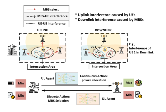
Figure 1: System model illustrating the interaction between the UEs and the MBSs, agents’ objectives and variables-of-control.

II-A Downlink Communication

Each of the MBS from $\mathcal{M}=\{1,2,...,M\}$ will be allocated to some UEs from $\mathcal{N}=\{1,2,...,N\}$. We define the size of the in-game graphics to be downloaded from the MBSs to the UEs as $D^{t}=\{D^{t}_{1},D^{t}_{2},...,D^{t}_{N}\}$, where $D^{t}_{i}$ represents the in-game data size to be downloaded from an MBS to UE $i\in\mathcal{N}$ at iteration $t$. In addition, the UE-MBS association is defined as: $\boldsymbol{c}^{t}=(c_{1}^{t},...,c_{N}^{t})$. Each of the $c_{i}^{t}$ where $i\in\mathcal{N}$ is allocated to an MBS $v$ where $v\in\mathcal{M}$ at iteration $t$. The effective signal, or signal-to-interference plus noise-ratio between a UE and its assigned MBS at step $t$ can be defined as:

$$\Gamma_{i}^{t}(\boldsymbol{c}^{t}) =\frac{g^{t}_{c_{i}^{t},i}p^{\text{d},t}_{c_{i}^{t},i}}{\sum\limits_{k\in\mathcal{N}\setminus\{i\}}g^{t}_{c_{k}^{t},i}p^{\text{d},t}_{c_{k}^{t},k}+B\sigma^{2}}$$

$$=\frac{g^{t}_{c_{i}^{t},i}p^{\text{d},t}_{c_{i}^{t},i}}{g^{t}_{c_{i}^{t},i}\sum\limits_{n\in\mathcal{N}\setminus\{i\}:c_{n}^{t}=c_{i}^{t}}p^{\text{d},t}_{c_{n}^{t},n}+\sum\limits_{j\in\mathcal{M}\setminus\{c_{i}^{t}\}}g^{t}_{j,i}\sum\limits_{k\in\mathcal{N}:c_{k}^{t}=j}p^{\text{d},t}_{j,k}+B\sigma^{2}},$$ (1)

where $p^{\text{d},t}_{c_{i}^{t},i}$ is the downlink transmission power provided by MBS $c_{i}^{t}$ to facilitate the downlink transmission of in-game graphical scenes to UE $i$ at transmission step $t$ (the superscript “d” means downlink). The channel gain of MBS $c_{i}^{t}$ and UE $i$ at transmission step $t$ is denoted by $g^{t}_{c_{i}^{t},i}$. $p^{\text{d},t}_{c_{n}^{t},n}$ is the downlink transmission power provided by MBS $c_{n}^{t}$ to facilitate the downlink transmission of in-game graphical scenes to UE $n\neq i$ at transmission step $t$. However, we assume the MBS to have sufficient downlink transmission power. Hence, we choose to not optimize the downlink transmission power as the amount of power assigned for the downlink transmission to each UE can be taken to be constant, regardless of number of UE. $p^{\text{d}}_{c_{k}^{t},k}$ is the downlink transmission power provided by MBS $c_{k}^{t}$ to facilitate the downlink transmission of in-game graphical scenes to UE $k$ at transmission step $t$. The channel gain of other MBS $c_{k}^{t}$ and UE $i$ is denoted by $g^{t}_{c_{k}^{t},i}$. We denote the bandwidth of each MBS and power spectral density to be $B$ and $\sigma^{2}$, respecitvely. Note that the power spectral density follows the additive white Gaussian noise. Fundamentally, $g^{t}_{c_{i}^{t},i}\cdot p^{\text{d},t}_{i}$ is the signal received at UE $i$ from MBS $c_{i}^{t}$ at iteration $t$, $\left[g^{t}_{c_{i}^{t},i}\sum\limits_{n\in\mathcal{N}\setminus\{i\}:c_{n}^{t}=c_{i}^{t}}p^{\text{d},t}_{c_{n}^{t},n}\right]$ is the intra-cell interference as a result of the communication between MBS $c_{i}^{t}$ and other UE $n\neq i$ to UE $i$, and $\sum\limits_{j\in\mathcal{M}\setminus\{c_{i}^{t}\}}g^{t}_{j,i}\sum\limits_{k\in\mathcal{N}:c_{k}^{t}=j}p^{\text{d},t}_{j,k}$ is the inter-cell interference caused by the signals of all other MBSs $j\neq c_{i}^{t}$ to UE $i$.

The downlink transmission rate from an MBS to UE $i$ is denoted as $r^{\text{d},t}_{i}$ at each transmission iteration $t$. This transmission rate is influenced by the signal-to-noise-ratio based on the Shannon-Hartley theorem [24]:

$$r_{i}^{\text{d},t}=B\cdot\log_{2}\left(1+\Gamma_{i}^{t}\right),$$ (2)

A higher downlink data transmission rate will reduce the downlink data transmission latency for a given in-game data size to be downloaded. The downlink transmission delay can be defined as:

$$\ell^{\text{d},t}_{i}=\frac{D^{t}_{i}}{r^{\text{d},t}_{i}}$$ (3)

where $D^{t}_{i}$ is the size of in-game data to be downloaded from an MBS to UE $i$ at transmission step $t$ and the resolution-impacted earning potential function $\omega(r^{\text{d},t}_{i})$ is influenced by the UE $i$’s SINR. Intuitively, a more efficient UE to MBS allocation results in a higher UE $i$ SINR, UE $i$ downlink transmission rate $r^{\text{d},t}_{i}$ (data transmitted per unit of time), and lower downlink transmission delay $\ell^{\text{d},t}_{i}$, at iteration $t$. A higher data transmitted per unit of time is translated to improved graphic resolution per unit of time, resulting in an enhancement in players’ in-game visuals, which translates to better in-game performance and hence, better resolution-influenced earning potential.

II-B Uplink Communication

In the uplink leg of the communication model, each player (UE) allocated to an MBS will upload its graphical changes to the previously downloaded Metaverse in-game scene data, to its assigned MBS. In the context of Play-to-Earn games, these in-game graphical changes could be induced by UEs’ physical-world actions. These graphical changes to the scenes are denoted $F^{t}=\{F^{t}_{1},F^{t}_{2},...,F^{t}_{N}\}$. We consider the intra-MBS and inter-MBS interference in the uplink leg, as well. Hence the signal-to-interference-ratio, or effective signal between MBS $v$ and UE $i$ at transmission step $t$ can be defined as:

$$\Lambda_{i}^{t}(\boldsymbol{p}^{\text{u},t}) =\frac{g^{t}_{i,c_{i}^{t}}\cdot p^{\text{u},t}_{i}}{\sum\limits_{k\in\mathcal{N}\setminus\{i\}}g^{t}_{k,c_{i}^{t}}p^{\text{u},t}_{k}+B\sigma^{2}}$$

$$=\frac{g^{t}_{i,c_{i}^{t}}\cdot p^{\text{u},t}_{i}}{\sum\limits_{n\in\mathcal{N}\setminus\{i\}:c_{n}^{t}=c_{i}^{t}}g^{t}_{n,c_{i}^{t}}p^{\text{u},t}_{n}+\sum\limits_{k\in\mathcal{N},j\in\mathcal{M}\setminus\{c_{i}^{t}\}:c_{k}^{t}=j}g^{t}_{k,c_{i}^{t}}p^{\text{u},t}_{k}+B\sigma^{2}},$$ (4)

where $p^{\text{u},t}_{i}$ (the superscript “u” means uplink) is UE $i$’s power selected to facilitate the uplink transmission of in-game data graphical changes at iteration $t$. $p^{\text{u},t}_{n}$ is other UE $n$’s power selected to facilitate the uplink transmission of in-game data graphical changes at iteration $t$. Essentially, the interference generated by UEs allocated to MBS $c_{i}^{t}$ is $\left[\sum\limits_{n\in\mathcal{N}\setminus\{i\}:c_{n}^{t}=c_{i}^{t}}g^{t}_{n,c_{i}^{t}}p^{\text{u},t}_{n}\right]$, and the interference generated by UEs not allocated to MBS $c_{i}^{t}$ is $\left[\sum\limits_{k\in\mathcal{N},j\in\mathcal{M}\setminus\{c_{i}^{t}\}:c_{k}^{t}=j}g^{t}_{k,c_{i}^{t}}p^{\text{u},t}_{k}\right]$. The uplink data rate $r^{u,t}_{i}$ can similarly be represented by $r_{i}^{\text{u},t}(\boldsymbol{p}^{\text{u},t})=B\cdot\log_{2}\left(1+\Lambda_{i}^{t}(\boldsymbol{p}^{\text{u},t})\right)$, where $B$ is the bandwidth of the transmitting UE $i$. As the number of UEs allocated to the same MBS increases, the SINR and hence rate of data transfer, decreases.

The uplink transmission latency of UE $i$ at transmission step $t$ can be formulated as:

$$\ell^{\text{u},t}_{i}=\frac{F^{t}_{i}}{r^{\text{u},t}_{i}}$$ (5)

where $F^{t}_{i}$ is the uplink in-game graphics data size of UE $i$ at transmission step $t$, $r^{\text{u},t}_{i}$ is the uplink data transmission rate of UE $i$ at transmission step $t$. UE $i$’s energy expenditure for the uplink transmission of in-game graphics data at transmission step $t$ can be formulated as:

$$E^{t}_{i}=p^{\text{u},t}_{i}\cdot\ell^{\text{u},t}_{i}.$$ (6)

We define $Q^{t}_{i}$ to be the UE device $i$ energy consumption as a percentage of the UE device $i$’s initial battery amount, at transmission step $t$. $Q^{t}_{i}$ can be defined as: $Q^{t}_{i}=\frac{E^{t}_{i}}{Bat^{0}_{i}}\cdot 100$. In this context, $Bat^{0}_{i}$ represents the UE $i$’s initial battery amount while $E^{t}_{i}$ represents UE $i$’s energy consumption, at transmission step $t$. Utilizing a UE device energy consumption as a percentage of the UE device’s initial battery charge is a natural choice. This is because normalized values are more conducive for training reinforcement learning agents. The control of uplink transmission power influences the uplink transmission latency, which influences fluidity. On the other hand, the selection of uplink transmission power also influences UE battery expenditure.

II-C UE Movement Patterns

We consider the network area to be a two-dimensional coordinate system, $x$-dimension and $y$-dimension, where the UEs and MBSs are positioned. At each given iteration step $t$, UE $i$ is located at $(\mathcal{X}^{t}_{i},\mathcal{Y}^{t}_{i})$. The locations of UEs are restricted to an area, $\mathcal{Y}^{t}_{i}\in[0,Y_{max}]$ and $\mathcal{X}^{t}_{i}\in[0,X_{max}]$. $\mathcal{X}^{t}_{i}$ refers to UE $i$’s position in the $x$-dimension at transmission step $t$, while $\mathcal{Y}^{t}_{i}$ refers to UE $i$’s position in the $y$-dimension at transmission step $t$. $X_{max}$ is the defined boundary in the $x$-dimension while $Y_{max}$ is the defined boundary in the $y$-dimension. After each round of data transmission (downlink followed by uplink), UEs will take steps $x$ and $y$ in both $x$-dimension and $y$-dimension, with the step size uniformly sampled from $(-x_{max},x_{max})$ and $(-y_{max},y_{max})$, respectively. $x_{max}$ refers to the maximum allowed distance a UE can move in a single transmission iteration in the $x$-dimension. $y_{max}$ refers to the maximum allowed distance a UE can move in a single transmission iteration in the $y$-dimension. The $x$-dimension position $\mathcal{X}^{t}_{i}$ can be defined as:

$$\mathcal{X}^{t}_{i}=\begin{cases}0,&\text{if }\mathcal{X}^{t-1}_{i}+x\leq 0,\\ X_{max},&\text{if }\mathcal{X}^{t-1}_{i}+x\geq X_{max},\\ \mathcal{X}^{t-1}_{i}+x,&\text{otherwise,}\end{cases}$$ (7)

Likewise, the $y$-dimension position $\mathcal{Y}^{t}_{i}$ can be defined as:

$$\mathcal{Y}^{t}_{i}=\begin{cases}0,&\text{if }\mathcal{Y}^{t-1}_{i}+y\leq 0,\\ Y_{max},&\text{if }\mathcal{Y}^{t-1}_{i}+y\geq Y_{max},\\ \mathcal{Y}^{t-1}_{i}+y,&\text{otherwise,}\end{cases}$$ (8)

II-D Problem formulation

To sum up, the MSP’s DL objective is to find the optimal UE-MBS allocation $\boldsymbol{c}^{t}$ which minimizes the total downlink latency $\ell^{\text{d},t}_{i}$ while maximizing the worst-case (lowest) resolution-influenced UE earning potential $\min_{i\in\mathcal{N}}\sum_{t=1}^{T}\omega(r^{\text{d},t}_{i})$ across all UEs. The number of transmission steps in an episode is denoted by $T$. We formulate our downlink utility function as:

$$\min_{\boldsymbol{c}^{t}} \left[q\cdot\left(\frac{1}{N}\sum_{i\in\mathcal{N}}\sum_{t=1}^{T}\ell^{\text{d},t}_{i}\right)-(1-q)\cdot b\cdot\min_{i\in\mathcal{N}}\sum_{t=1}^{T}\omega(r^{\text{d},t}_{i})\right],$$ (9)

$$s.t.~{}~{} c_{i}^{t}=v\in\mathcal{M},\forall t\in\mathcal{T},~{}\forall i\in\mathcal{N},$$ (10)

where $\mathcal{T}$ represents the set of all transmission steps in an episode. Our resolution-impacted in-game profit is motivated by a recent work [25] and is modeled as: $\omega(r^{\text{d},t}_{i})=P\cdot\ln\left(1+{r^{\text{d},t}_{i}}\right)$, where $P$ is the player-specific profitability factor (using such logarithmic function as the utility also appears in the classical work on crowdsourcing [26]). The logarithmic function has a increasing first-order derivative and decreasing second-order derivative property. When applied to the Play-to-Earn profit model, the increasing first-order derivative implies that UE in-game profits increases as the downlink transmission rate increases, while the decreasing second-order derivative implies that the rate of profit increment decreases as the downlink transmission rate increases. It is natural to model our profit model as such as a larger downlink data (resolution) per unit time improves UEs’ visibility within the games, allowing them to perform better and reap higher profits. However, as the resolution improves, its impact on UE’s visibility and hence earnings, decreases, resulting in a slowing rate of profit increment with increasing downlink transmission rate. The constraint (10) ensures that each UE is assigned to one MBS in each transmission step. $q$ is a factor which determines the weighting on $\sum_{i\in\mathcal{N}}\sum_{t=1}^{T}\ell^{\text{d},t}_{i}$ and $b\cdot\min_{i\in\mathcal{N}}\sum_{t=1}^{T}\omega(r^{\text{d},t}_{i})$. $b$ is a factor that places both terms $\sum_{i\in\mathcal{N}}\sum_{t=1}^{T}\ell^{\text{d},t}_{i}$ and $b\cdot\min_{i\in\mathcal{N}}\sum_{t=1}^{T}\omega(r^{\text{d},t}_{i})$ on the same measurement unit.

On the other hand, MSP’s UL objective is to obtain the optimal UE uplink power $p^{\text{u},t}$ that minimizes the total latency of the data uplink transmissions $\ell^{\text{u},t}_{i}$ and worst-case (greatest) UE device energy expenditure $Q^{t}_{i}$. We formulate our uplink utility function as:

$$\min_{\boldsymbol{p^{t}}} \left[h\cdot\left(\frac{1}{N}\sum_{i\in\mathcal{N}}\sum_{t=1}^{T}\ell^{\text{u},t}_{i}\right)+(1-h)\cdot f\cdot\max_{i\in\mathcal{N}}\sum_{t=1}^{T}Q^{t}_{i}\right],$$ (11)

$$s.t.~{}~{} \sum_{t=1}^{T}Q^{t}_{i}\leq 100,\forall i\in\mathcal{N}.$$ (12)

where $\ell^{\text{u},t}_{i}$ is the player (UE) $i$’s uplink data transmission delay at transmission iteration $t$. $h$ is a factor that determines the weighting on $\sum_{i\in\mathcal{N}}\sum_{t=1}^{T}\ell^{\text{u},t}_{i}$ and $f\cdot\max_{i\in\mathcal{N}}\sum_{t=1}^{T}Q^{t}_{i}$. Scaling factor $f$ in the objective function is to place both terms $\sum_{i\in\mathcal{N}}\sum_{t=1}^{T}\ell^{\text{u},t}_{i}$ and $f\cdot\max_{i\in\mathcal{N}}\sum_{t=1}^{T}Q^{t}_{i}$ on the same measurement unit. Finally, constraint (12) ensures that the UE battery consumption has to be less than 100% (or battery charge (%) has to be greater than 0) for the uplink transmission.

III Reinforcement learning settings

We assign two reinforcement learning agents, one (DL agent) controlling the downlink transmission UE-MBS allocation, and the other (UL agent) controlling the uplink transmission power selection. The DL agent and UL agent serve their objectives (9) and (11), respectively.

III-A State

For the DL agent’s observation state $s^{\text{d}}$, we choose to include 1) channel gain between UEs and MBSs: $g^{t}_{v,i}$, 2) in-game scene DL data size at each transmission iteration $t$: $D^{t}_{i}$, as $D^{t}_{i}$ influences latency $\ell^{\text{d},t}_{i}$, and $g^{t}_{v,i}$ influences both data DL transmission latency $\ell^{\text{d},t}_{i}$ and worst-case (lowest) resolution-influenced in-game earning potential $\min_{i\in\mathcal{N}}\sum_{t=1}^{T}\omega(r^{\text{d},t}_{i})$.

For the UL agent’s observation state $s^{\text{u}}$, we choose to include 1) channel gain between UEs and MBSs: $g^{t}_{v,i}$, as it influences data UL transmission rate, latency $\ell^{\text{u},t}_{i}$ and uplink transmission battery consumption $Q^{t}_{i}$. As we consider the cumulative battery amount consumed by UE devices and are enforcing that each UE has positive battery-charge to continue the uplink transmission at each transmission iteration step $t$, we have to include 2) UE device battery life (%): $\left[\frac{Bat^{t}_{i}}{Bat^{0}_{i}}\cdot 100\right]$ , as UE device battery life changes in each iteration.

III-B Action

In the DL communication model, the DL agent’s action involves deciding the UE to MBS assignment. The UE to MBS allocation action at transmission step $t$ is defined as: $a^{\text{d},t}=\textbf{c}^{t}=\{c_{1}^{t},...c_{N}^{t}\}.$ In the UL communication model, the UE device power for uplink data transmission at transmission step $t$ is defined as: $a^{\text{u},t}=\textbf{p}^{\text{u},t}=\{p^{\text{u},t}_{1},...,p^{\text{u},t}_{N}\}$. $p^{\text{u},t}_{i}$ represents UE $i$’s selected power for the uplink data transmission at transmission step $t$.

III-C Reward

For the downlink communication model, the reward given to the DL agent at transmission step $t$ is given as such: $R^{\text{d},t}=-q\cdot\frac{\sum_{i\in\mathcal{N}}\ell^{\text{d},t}_{i}}{N}+\left(1-q\right)\cdot b\cdot\min_{i\in\mathcal{N}}\sum_{\tau=1}^{t}\omega(r^{\text{d},t}_{i})$ if the total battery consumed as of transmission step $t$ $\sum_{\tau=1}^{t}Q^{t}_{i}\leq 100$. Otherwise, $R^{\text{d},t}=\varrho$, where $\varrho$ is a very large penalty. $\tau$ denotes the summation of index. For the uplink communication model, the reward issued to the UL agent at transmission step $t$ is defined as: $R^{\text{u},t}=-h\cdot\frac{\sum_{i\in\mathcal{N}}\ell^{\text{u},t}_{i}}{N}+\left(1-h\right)\cdot f\cdot\min_{i\in\mathcal{N}}\sum_{\tau=1}^{t}Q^{t}_{i},$ if the total battery consumed as of transmission step $t$ $\sum_{\tau=1}^{t}Q^{t}_{i}\leq 100$. Otherwise, $R^{\text{u},t}=\varrho$, where $\varrho$ is a very large penalty. The intuition for the downlink and uplink reward assignment follows the utility function in Equations (9) and (11), respectively.

IV Methodology

Inspiration. In our problem definition, the Metaverse Service Provider (MSP) aims to minimize the latency of the downlink and uplink data transmission, and worst-case (greatest) UE uplink transmission battery charge expenditure, while maximizing the worst-case (lowest) UE’s resolution-impacted earning potential. Given that the MSP has multiple objectives, rudimentary reinforcement learning agents employed struggle to achieve them and may fail to achieve convergence. One reason is that independent agents act in their own interest, choosing the best actions to maximize their own rewards, even if it is at the expense of other agents. In a mixed-cooperative scenario as proposed in our study where each agent acts in its interest, agents’ greedy actions may result in sub-optimal action solutions learned across all agents. To tackle this issue, we proposed a novel multi-input, multi-objective (head) critic which provides actors with actor-centric guidance, facilitating the actors in breaking down complex objectives into simpler ones. A (multi) dual-head critic refers to a critic model with (multiple) two distinct neural network input layers, each to accommodate to the input state of each agent, while sharing a common neural network backbone. The critic head serving the uplink actor beacons the UL actor in (i) minimizing the UL transmission delay and UE battery consumption in the uplink transmissions. The critic head serving the downlink actor beacons the DL actor in (ii) minimizing the DL transmission delay and (iii) maximizing the UE resolution-influenced in-game earning potential. To ensure that each agent involved learns a jointly optimal solution, the loss value of each critic’s head is shared (summed) for the joint update of the critic model.

In the following section, we will introduce the PPO algorithm, its mechanism as it is the backbone algorithm in which our MALS algorithm is built upon.

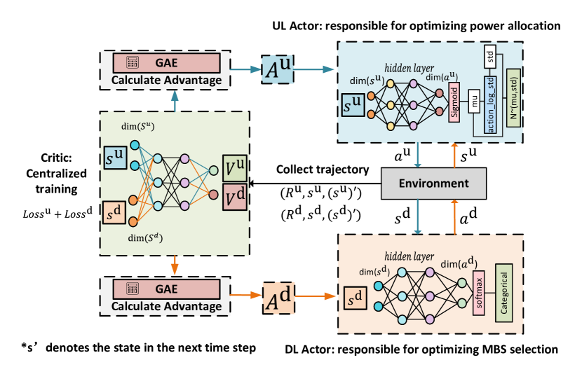
Figure 2: Reinforcement Learning Multi-Agent-Loss-Sharing Proximal Policy Optimization (MALS-PPO) structure and model update in a single time step.

IV-A Proximal Policy Optimization (PPO)

As we emphasize on developing a multi-agent RL model to tackle asymmetric tasks, asynchronously, policy stability is essential. The Proximal Policy Optimization (PPO) algorithm proposed by OpenAI [27] is an enhancement of the traditional policy gradient algorithm. PPO has better sample efficiency by using a separate policy for sampling, and is more stable by embedding a policy constraint.

In summary, PPO has two main characteristics in its policy network (Actor): (1) Increased sample efficiency. PPO uses two separate policies for sampling trajectories and optimization to improve sample efficiency. $\pi_{\theta}$ and $\pi_{\theta^{{}^{\prime}}}$ are defined as the evaluation policy and data-sampling policy, respectively. $\theta$ is the parameter for the evaluation policy and $\theta_{{}^{\prime}}$ is the parameter of the data sampling policy.

(2) Policy constraint. After switching the data sampling policy from $\pi_{\theta}$ to $\pi_{\theta^{{}^{\prime}}}$, an issue still remains. Although the expected value of the evaluation and data sampling policy is similar, their variances are starkly distinct. A policy constraint is implemented in the form of threshold clipping and the state-action pair expectation is defined as: $\mathbb{E}_{(s^{t},a^{t})\sim\pi_{\theta^{{}^{\prime}}}}[\min\{\frac{\pi_{\theta}(a^{t}|s^{t})}{\pi_{{\theta^{\prime}}}(a^{t}|s^{t})},\operatorname{clip}(\frac{\pi_{\theta}(a^{t}|s^{t})}{\pi_{{\theta^{\prime}}}(a^{t}|s^{t})},1-\epsilon,1+\epsilon)\}\cdot A^{t}]$, where $A^{t}$ is the advantage value. Gradient ascent is then used to improve the policy:

$$\Delta\theta=\mathbb{E}_{(s^{t},a^{t})\sim\pi_{\theta^{{}^{\prime}}}}[\Delta\min\{\frac{\pi_{\theta}(a^{t}|s^{t})}{\pi_{{\theta^{\prime}}}(a^{t}|s^{t})},\operatorname{clip}(\frac{\pi_{\theta}(a^{t}|s^{t})}{\pi_{{\theta^{\prime}}}(a^{t}|s^{t})},1-\epsilon,1+\epsilon)\}\cdot A^{t}].$$ (13)

With regards to the critic network, all actors under the PPO algorithm share a similar critic network model. Hence, the authors of  [27] formulate the critic loss to be:

$$L(\phi)=(V_{\phi}(s^{t})-A^{t}+\gamma V_{\phi_{targ}}(s^{t}))^{2}.$$ (14)

$\phi$ is the parameter of the critic model. The state-values $V_{\phi}(s^{t})$ and $V_{\phi_{targ}}(s^{t})$ are estimated with the critic model and the target critic model, respectively. Essentially, the critic model utilizes the loss function $L(\phi)$ to update the critic network.

IV-B Multi-Agent-Loss-Sharing (MALS)

In this paper, MALS is an RL structure that can accommodate asymmetric actors of different action spaces. We adopt PPO as the underlying algorithm of MALS and utilize two actors, one which has a discrete UE-MBS allocation action, and the other which has a continuous power selection action. The MALS algorithm adopts a multi-head critic, with each head serving as a beacon to an actor.

Transmission mechanism: In a single transmission with one DL-UL iteration, the downlink state $s^{\text{d},t}$ will be observed by the DL agent. The DL agent will then choose an action $a^{\text{d},t}$ based on its policy and observed state. This action causes an impact on the environment, and a DL reward $R^{\text{d},t}$ is issued to the DL agent in accordance to the merit of its actions. The altered environment consequently influences the UL state $s^{\text{u},t}$ observed by UL agent. Based on its policy, the UL agent will choose an action $a^{\text{u},t}$ which corresponds to the current observed state. This action by the UL agent influences the environment, and yields the UL agent a corresponding reward $R^{\text{u},t}$ and the next DL state $s^{\text{d},t+1}$. After several iterations, the rewards ($R^{\text{d},t},R^{\text{u},t}$) with states ($s^{\text{d},t},s^{\text{u},t}$) and their corresponding next states ($s^{\text{d},t+1},s^{\text{u},t+1}$) will be sent to the multi-head critic. The critic will then utilize these rewards, states, and next iteration states to calculate state-value $V$ and advantage value $A$ to update the actor network parameters. This transmission mechanism is illustrated in Fig 2.

Asymmetric Actor: In MALS, there are two Actors: one arranges UE-MBS allocation in the downlink transmission, and the other selects the UE power for the uplink transmission. The UE-MBS allocation is a discrete case selection and hence probabilities are computed for each action based on the DL agent policy [28]. The transmission power selection in the UL stage falls along a continuum and hence a probability distribution over the output power values are learnt by the UL agent.

In addition to having distinct action space types, the agents have different objectives to tackle. The DL and UL agents are given only portions of the overarching objective that they control as this is to avoid “confusing” agents with rewards that they do not control. For instance, in our work, we do not present the UL agent with rewards pertaining to downlink transmission latency as downlink transmission latency is not within the UL agent’s control.

In MALS, $\theta^{\text{d}}$ and $\theta^{\text{u}}$ are the network weights of DL agent and UL agent, and the gradients $\Delta\theta^{\text{d}}$, $\Delta\theta^{\text{u}}$ of the DL agent and UL agent are:

$$\Delta\theta^{\text{u}}=\mathbb{E}_{(s^{\text{u},t},a^{\text{u},t})\sim\pi_{{\theta^{\text{u}}}^{\prime}}}[\triangledown f^{t}(\theta^{\text{u}})A^{\text{u}}(s^{\text{u},t})],$$ (15)

$$\Delta\theta^{\text{d}}=\mathbb{E}_{(s^{\text{d},t},a^{\text{d},t})\sim\pi_{{\theta^{\text{d}}}^{\prime}}}[\triangledown f^{t}(\theta^{\text{d}})A^{\text{d}}(s^{\text{d},t})],$$ (16)

where $f^{t}(\theta)=\min\{\frac{\pi_{\theta}(a^{t}|s^{t})}{\pi_{{\theta^{\prime}}}(a^{t}|s^{t})},\operatorname{clip}(\frac{\pi_{\theta}(a^{t}|s^{t})}{\pi_{{\theta^{\prime}}}(a^{t}|s^{t})},1-\epsilon,1+\epsilon)\}$ in the case of PPO, in which $\epsilon$ is the clipping parameter, and $A(\cdot)$ is the advantage function of both UL and DL agents.

Advantage function. We utilize the state-value function ($V$) and the truncated version of the Generalized Advantage Estimation (GAE) [29] method to calculate the advantage values. The policy is then executed for $\bar{T}$ time steps, where $\bar{T}$ is the number of steps in a trajectory. A trajectory of $\bar{T}$ number of steps represents the path of an agent through the state space up till horizon $\bar{T}$. The advantage value in our work can be calculated as:

$$A^{\text{u},t}=\delta^{\text{u},t}+(\gamma\lambda)\delta^{\text{u},t+1}+...+(\gamma\lambda)^{\bar{T}-1}\delta^{\text{u},t+\bar{T}-1},\text{ for}~{}\delta^{\text{u},t}=R^{\text{u},t}+\gamma V_{\phi_{targ}}(s^{\text{u},t+1})-V_{\phi_{targ}}(s^{\text{u},t}),$$ (17)

$$A^{\text{d},t}=\delta^{\text{d},t}+(\gamma\lambda)\delta^{\text{d},t+1}+...+(\gamma\lambda)^{\bar{T}-1}\delta^{\text{d},t+\bar{T}-1},\text{ for}~{}\delta^{\text{d},t}=R^{\text{d},t}+\gamma V_{\phi_{targ}}(s^{\text{d},t+1})-V_{\phi_{targ}}(s^{\text{d},t}),$$ (18)

where $\bar{T}$, $\gamma$, and $\lambda$ denote the trajectory length, discount factor, and GAE parameter, respectively. $\phi$ and $\phi_{targ}$ are the parameters of the critic model and the target model, respectively.

Multi-head Critic: We proposed an asymmetric problem in our work, where each agent optimizes different variables and has different objectives. A multi-head critic caters to the asymmetric actors by providing personalized calculations of state-values $V_{\phi}^{u},V_{\phi}^{d}$ using a neural network with two heads. Each critic head produces a loss value corresponding to the state-value that it produces, and the loss values of the critic heads are weighted-summed ($\kappa_{1}$ and $\kappa_{2}$) to give a conclusive loss value as follows:

$$L^{\text{u}}(\phi)=(V_{\phi}(s^{\text{u},t})-\gamma V_{targ}^{\text{u},t}))^{2},$$ (19)

$$L^{\text{d}}(\phi)=(V_{\phi}(s^{\text{d},t})-\gamma V_{targ}^{\text{d},t}))^{2},$$ (20)

$$L(\phi)=\kappa_{1}\times L^{\text{u}}(\phi)+\kappa_{2}\times L^{\text{d}}(\phi).$$ (21)

The specific values of $\kappa_{1}$ and $\kappa_{2}$ will be specified in the experiments. The multi-head critic’s model parameter is updated with the loss in Equation (21) to improve the critics model in guiding the asymmetric actors. The MALS algorithm is detailed in Algorithm 1.

Algorithm 1 MALS-PPO (proposed RL structure)

0:  critic model $\phi$ and target model $\phi_{targ}$, downlink actor model $\theta^{\text{d}}$ and sampling model $(\theta^{\text{d}})^{\prime}$, uplink actor model $\theta^{\text{u}}$ and sampling model $(\theta^{\text{u}})^{\prime}$, initial state $s^{\text{d},1}$.

1:  $s^{\text{d},t}\leftarrow s^{\text{d},1}$;

2:  for iteration $t=1,2,...$ do

3:     DL agent executes action according to $\pi_{(\theta^{\text{d}})^{\prime}}(a^{\text{d},t}|s^{\text{d},t})$;

4:     Get reward $R^{\text{d},t}$ and uplink state $s^{\text{u},t}$;

5:     UL agent executes action according to $\pi_{(\theta^{\text{u}})^{\prime}}(a^{\text{u},t}|s^{\text{u},t})$;

6:     Get reward $R^{\text{u},t}$ and next step downlink state $s^{\text{d},t+1}$;

7:     DL agent executes action according to $\pi_{(\theta^{\text{d}})^{\prime}}(a^{\text{d},t+1}|s^{\text{d},t+1})$;

8:     Get reward $R^{\text{d},t+1}$ and uplink state $s^{\text{u},t+1}$;

9:     if iteration $t\geq 2$ then

10:        Sample ($s^{\text{d},t},a^{\text{d},t},s^{\text{u},t},a^{\text{u},t},R^{\text{d},t},R^{\text{u},t},s^{\text{d},t+1},s^{\text{u},t+1}$) iteratively till end of episode;

11:     end if

12:     $s^{\text{d},t}\leftarrow s^{\text{d},t+1}$, $s^{\text{u},t}\leftarrow s^{\text{u},t+1}$, $a^{\text{d},t}\leftarrow a^{\text{d},t+1}$, $R^{\text{d},t}\leftarrow R^{\text{d},t+1}$;

13:     Compute advantages $\{A^{\text{d},t},A^{\text{u},t}\}$

14:     Compute target values {$V^{\text{d},t}_{targ},V^{u,t}_{targ}$}

15:     for $k$ = $1,2,...,K$ do

16:        Assign samples into training groups;

17:        for each training group do

18:           Compute UL and DL actor model gradients: $\triangledown\theta^{\text{d}},\triangledown\theta^{\text{u}}$

19:           Apply gradient ascent on $\theta^{\text{d}}$ using $\triangledown\theta^{\text{d}}$ by Eq. (16)

20:           Apply gradient ascent on $\theta^{\text{u}}$ using $\triangledown\theta^{\text{u}}$ by Eq. (15)

21:           Update the critic model with loss from Eq. (21)

22:        end for

23:     end for

24:     Update the critic target model parameters $\phi_{targ}$ with the critic model parameters $\phi$ every $C$ steps where $C$ is the critic model update interval;

25:  end for

V Experiments

We conduct several experiments and showcase the superiority of our MALS RL structure in handling asymmetric and asynchronous problems. We first discuss the numerical settings for the experiments we conduct. We then show how the proposed MALS algorithm is effective in improving resource management when compared against commonly adopted metrics. We then compare the proposed MALS model with baseline algorithms (i) independent dual agent (IDA) [30] and (ii) Centralized Training and Decentralized Execution multi-agent model (CTDE) [31]. Finally, we vary the weighting on each variable in the DL and UL agents’ objective functions to study the performance of the MALS model on varying variable weights and their implications on the model performance.

V-A Baseline algorithms

We pit the baseline algorithms (IDA and CTDE) against our proposed MALS model in tackling the asymmetric and asynchronous task. The IDA model encompasses two agents which are only dependent on the states each agent observes. The reward for the UL and DL agent are $R^{\text{u},t}$ and $R^{\text{d},t}$, respectively. The CTDE model is based on [8] which utilizes two actors and identical critics. The rewards obtained by the critics are summed to produce an overall reward of $R^{\text{u},t}+R^{\text{d},t}$.

V-B Configuration

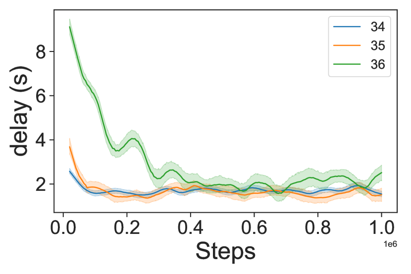
(a) Average downlink delay.

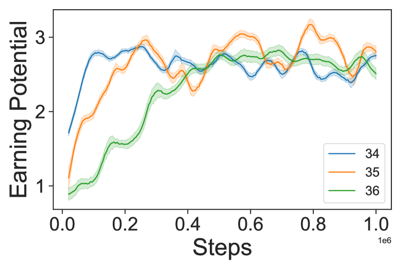
(b) Average UE earning potential.

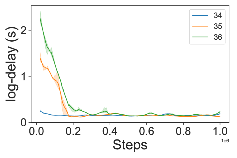
(c) Average uplink delay.

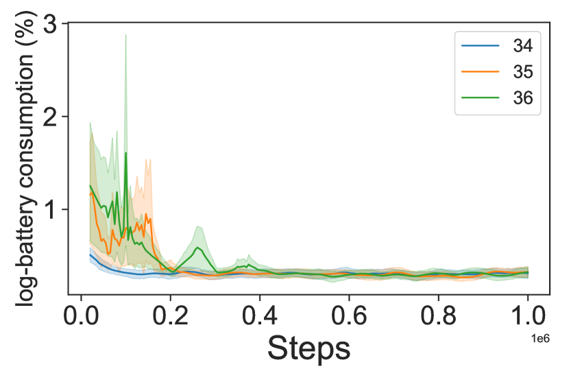
(d) Average battery consumption.

Figure 3: Key metrics performance obtained by MALS across training steps.

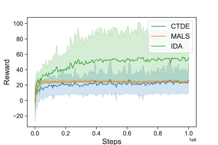
(a) Downlink reward for 3 MBS, 4 UE.

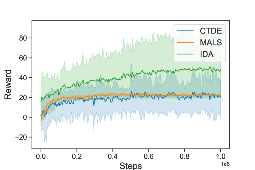
(b) Downlink reward for 3 MBS, 5 UE.

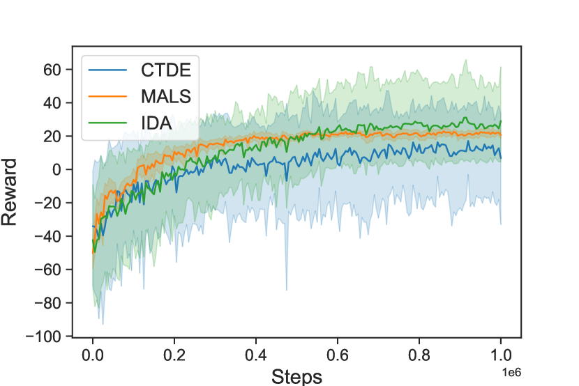
(c) Downlink reward for 3 MBS, 6 UE.

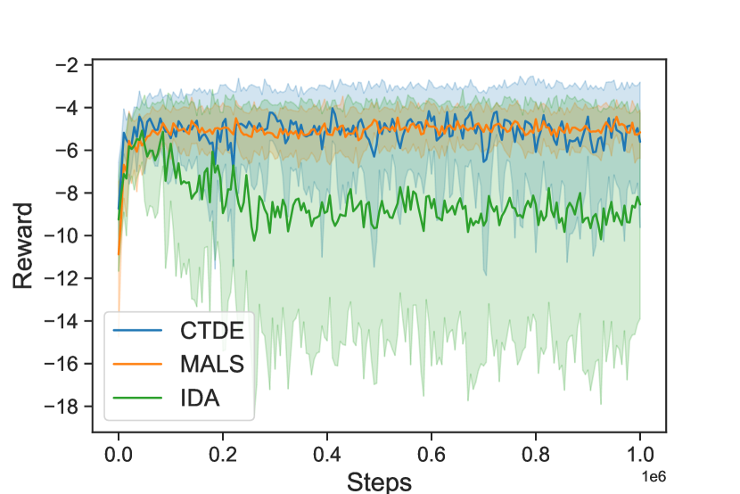
(d) Uplink reward for 3 MBS, 4 UE.

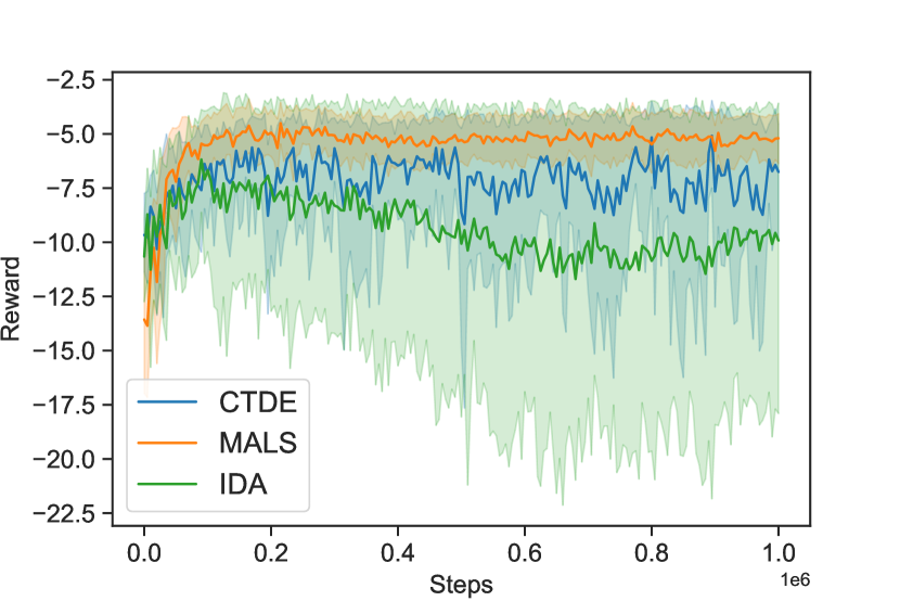
(e) Uplink reward for 3 MBS, 5 UE.

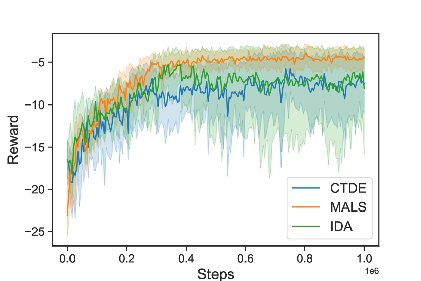
(f) Uplink reward for 3 MBS, 6 UE.

Figure 4: Uplink and downlink agent rewards obtained for MALS model, Independent Dual Agent model, CTDE model, across congestion settings and seed 0 to 9. Bands within the graph indicate the range of reward values obtained across the seeds.

We design an experiment with three scenarios: 3 MBSs and 4 to 6 UEs to test our proposed Multi-Agent-Loss-Sharing (MALS) reinforcement learning-based method. $T$ which is defined as the number of transmission steps within an episode is set as $100$. Exhaustive search is an infeasible method to optimize the UE-MBS assignment as the sequential nature of our proposed problem renders the complexity to be $(M^{N})^{T}$, where $M$ is the number of MBS, $N$ is the number of UEs, and $T$ is the number of transmission iterations in an episode. The bandwidth $B$ is set as $10$ MHz, while the noise $\sigma^{2}$ is set as $100$ dBm. The output power by the MBS for the downlink transmission is set to be within $(1.5,2.0)$ Watt. We initialize the locations of the MBSs and UEs to be random, within a 100m by 100m area. The Metaverse in-game graphic size $D_{i}^{t}$ of each UE at every step is uniformly distributed between $800$ and $1000$ Mb. We set $P$, $b$ and $f$ to be 100, 50 and 75, respectively, after empirical tuning, and $h$ and $q$ to be 0.5. $P$ is defined in subsection V-B, $b$, $f$, $h$ and $q$ are defined in subsection II-D. We set the values of both $\kappa_{1}$ and $\kappa_{2}$ from Equation (21) to be $0.5$. We set the maximum distance UEs can move in each iteration ($x_{max}$ and $y_{max}$) to be 10m. The ADAM optimizer [32] is utilized for the algorithms we study. We trained the models for 1,000,000 iterations (steps) for all congestion settings. We conducted the training and simultaneous evaluation of the models for each configuration at different seed settings: seed 0 to seed 9.

V-C Result analyses

V-C1 MALS model convergence

In training our MALS model, all three configurations (i) 3 MBS, 4 UE, (ii) 3 MBS, 5 UE and (iii) 3 MBS, 6 UE showed a general increment of achieved test reward for both the downlink and the uplink models (shown in Figure 4) and improvement in the underlying metrics (shown in Figure 3). Note that at the start of training, the 3 MBS, 4 UE configuration received a higher reward than the 3 MBS, 5 UE and 3 MBS, 6 UE as there is less complexity in its scenario, allowing the model to converge quicker and achieve a higher reward. Conversely, a more complex model like 3 MBS, 6 UE converges slower due to the higher complexity of the action space and having more UEs to manage. Overall, the improvement in both the downlink and uplink reward signifies that the overall utility function for both agents are improving. More explicitly, training of the downlink agent and uplink agent improves its UE-MBS allocation and output power allocation, respectively.

Downlink. The gradual increment in the downlink reward, as training progresses, can be attributed to the decrease in in-game downlink transmission time (shown in Figure 3(a)) and increase in worst-case (lowest) earning potential of the UEs (shown in Figure 3(b)) with each training step. These observations directly reflect that the downlink agent is allocating UE-MBS more efficiently, achieving a higher downlink data transfer rate which decreases the downlink latency and improves the worst-case (lowest) earning capability of the UEs. We should note that the simpler configurations such as 3 MBS, 4 UE and 3 MBS, 5 UE still achieves better rewards, shorter downlink latency and higher worst-case earnings in the final training steps as it is easier to obtain an optimal solution for simpler configurations as opposed to more complex scenarios such as 3 MBS, 6 UE.

Uplink. Similarly, we note that the improvement of the uplink reward received by the uplink agent, as training progresses, can be attributed to the more optimal use of UE transmission output power for the uplink transmission, resulting in a lower average uplink delay (shown in Figure. 3(c)) and lower worst-case (greatest) battery charge expenditure. This is reflected in Figure 3(d). Note that both the UL transmission delay and worst-case (greatest) battery charge expenditure are shown in log-scale as the initial uplink transmission delay and worst-case (greatest) battery charge expenditure at the start of training were very large.

V-C2 Comparison with other reinforcement learning model structures

We study how (i) our proposed model (MALS model structure) compared to other reinforcement learning-based structures. We adopt two reinforcement learning-based model structures; the most intuitive (ii) independent dual agent (IDA) (which employs two individual agents in which information transfer is only via the states), and (iii) CTDE (which is the framework used for multi-agent reinforcement learning [8]).

Our proposed model (MALS model structure) achieves a smooth convergence for each configuration, exhibiting a narrow range of downlink and uplink rewards, across different seeds (shown in Figure 4). The solid line in the charts represents the mean reward of the different seed settings, for each configuration. The color hue bands around the solid line represent the minimum (lower bound) and maximum (upper bound) of the rewards received. We observe that our proposed model obtains approximately around 20 points for the downlink reward and -4 for the uplink reward for each configuration. The narrow bands indicate that the proposed model is stable across the different seed settings, for each of the configurations.

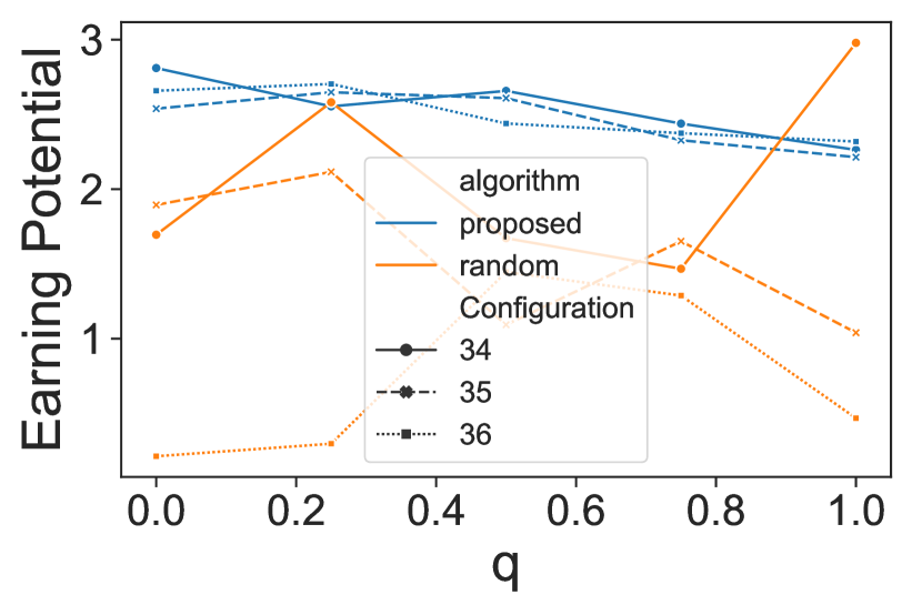
(a) Earning potential wrt $q$.

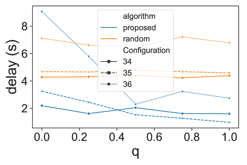
(b) Downlink delay wrt $q$.

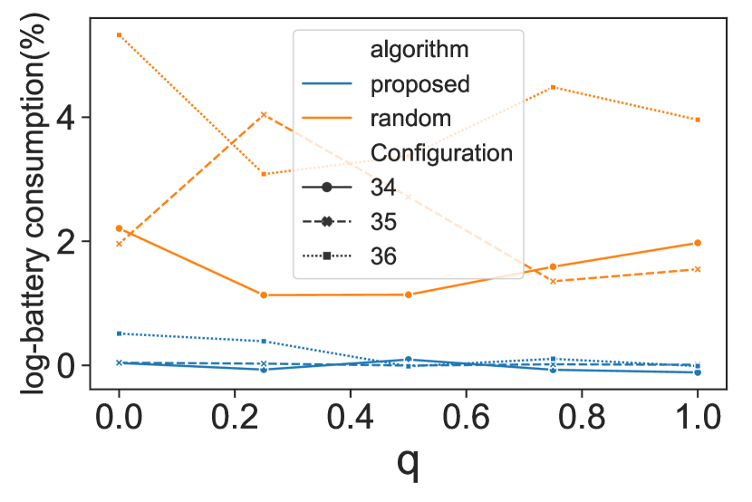
(c) Battery consumption wrt $q$.

(d) Uplink delay values wrt $q$.

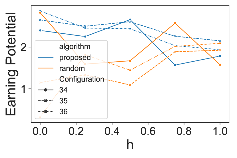
(e) Earning potential wrt $h$.

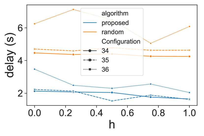
(f) Downlink delay wrt $h$.

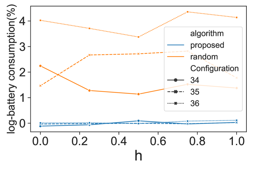
(g) Battery consumption wrt $h$.

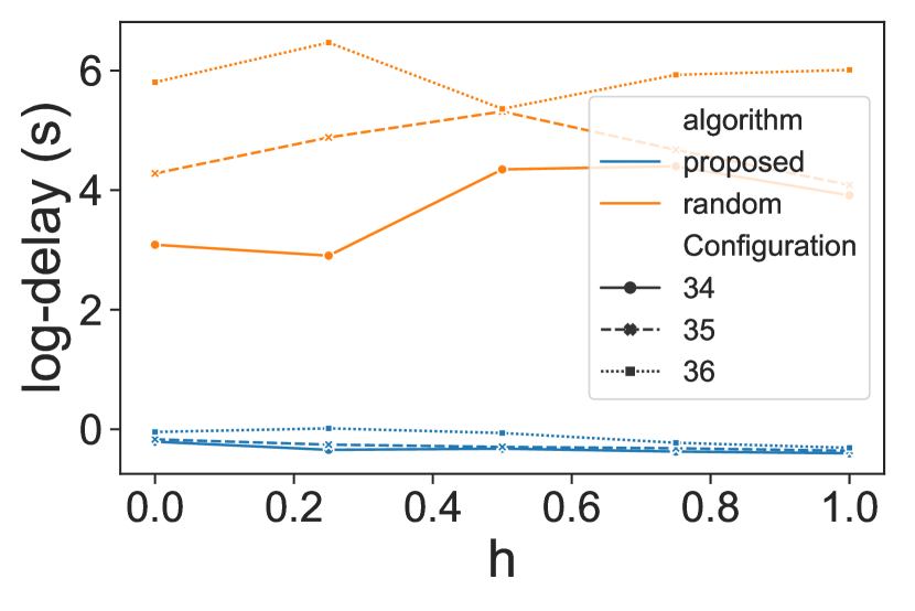
(h) Uplink delay wrt $h$.

Figure 5: Metric values with respect to (wrt) different $q$ and $h$

On the other hand, the (ii) IDA model took significantly more steps to converge (shown in Figure 4). We observe that the independent dual agents model obtained significantly higher downlink reward in the 3 MBS, 4 UE and 3 MBS, 5 UE configuration, with a mean of approximately 50 points for the 3 MBS, 4 UE configuration and for the 3 MBS, 5 UE configuration. However, the variance of downlink rewards obtained is much larger for the independent dual agents model, with rewards as high as sub-hundred in the 3 MBS, 4 UE configuration, and as low as in the tens for the 3 MBS, 6 UE configuration. This indicates instability and hyper-sensitivity of the model when handling different seed settings and minute changes in environment. Nevertheless, the excellence of the independent model observed in the downlink reward of some seeds seems to be reflected as a compromise in the performance of the independent dual agent’s uplink reward. From Figure 4(d), 4(e), we observe that the average 3 MBS, 4 UE and 3 MBS, 5 UE configurations have a slight improvement in the uplink rewards in the early training steps, followed by a subsequent decline in rewards obtained. The variance of the rewards obtained for each configuration enormous as well, with the highest rewards obtained being close to 0 points, while the lowest rewards obtained being south of -20 points. Some seeds show an evident decline in uplink reward obtained as training proceeds. This shows a convergence failure for some of these seeds in the independent dual-agent model. It is apparent that the downlink agent’s rewards are prioritised over the uplink agent’s rewards in this case, which renders the IDA model unsuitable for real-world deployment.

The (iii) CTDE model achieves comparable performance to our proposed methods (MALS) for the 3 MBS, 4 UE configuration for both the downlink and uplink rewards (shown in Figure 4(a), 4(d)), but achieved lackluster performance for both 3 MBS, 5 UE and 3 MBS, 6 UE configurations for both the downlink and uplink rewards (shown in Figure 4(b), 4(c), 4(e), 4(f)). The CTDE produces a large variance of downlink and uplink reward outputs across the different seeds, albeit not as severe as the IDA model, as the model still converges in all seeds. However, the large variance and sub-par rewards obtained renders the CTDE inferior to our proposed methods due to its poorer performance, instability and unreliability.

V-C3 Weighting Emphasis On Joint Utility function

When dealing with joint optimization problems, it is essential for us to observe how our proposed model handles the varying weights on variables and their influence on variables of interest, as this provides future research insights on multi-agent joint utility function design.

Downlink weight analysis. Firstly, we vary the weight $q$ in the downlink reward $R^{\text{d},t}$ in subsection III-C with values from the set of {0, 0.25, 0.50, 0.75, 1}. We then take the average results of the last 20,000 training steps the different variables of interest (downlink delay, worst-case (lowest) earning potential, uplink transmission delay, worst-case (greatest) battery charge expenditure). These averaged results are then compared with a random policy that assigns the downlink UE-MBS allocation and uplink power output randomly. We compare our proposed model with a random policy to show how our proposed model adds value in optimizing UE-MBS allocation and power selection. Please refer to the Appendix for the complete comparison with the reinforcement learning model structures discussed (IDA and CTDE). We do not focus on them as they have been shown to produce unreliable performance with high variances (in Fig. 6 and 7).

Across all $q$ weight values, the earnings of our proposed MALS model outperform random allocation (with the exception of $q$ = 1), which shows that our model improves the earning capability of the UEs (shown in Figure 5(a)). It is not surprising that the random policy agent allows users to earn higher earnings at $q$ = 1 than our model as higher $q$ values place more weight emphasis on downlink delay, and less weight emphasis on the worst-case (lowest) UE in-game earning capability. At $q$ = 1, the downlink agent in our proposed model focuses entirely on minimizing downlink latency, with no regard for maximizing the worst-case (lowest) UE earning capabilities. Another point to note is that, across each scenario configuration of our proposed method, the worst-case (lowest) UE earning potential decreases as $q$ increases. This is expected as the agent places more weight emphasis on minimizing downlink latency and less weight emphasis on maximizing the worst-case (lowest) UE earning potential at higher $q$ values.

We observe that our proposed downlink latency across different configurations, across different $q$ values, are much lower than the random policy with the exception of the 3 MBS, 6 UE configuration at $q$ = 0 (shown in Figure 5(b)). Poorer performance in 3 MBS, 6 UE configuration is not unexpected as at $q$ = 0, there is no weight emphasis on minimizing downlink delay, and whole emphasis on maximizing the worst-case (lowest) UE earning potential. Another thing to note is that the overall downlink latency for each configuration decreases as $q$ increases. This is because a higher value of $q$ increases its weight emphasis on minimizing agent downlink delay.

It may seem that the uplink model factors such as uplink delay and uplink battery charge consumption are not directly influenced by $q$ since $q$ is the weighting parameter that controls downlink model factors such as worst-case (lowest) UE earning ability and downlink latency. However, we note that for both the uplink transmission delay and worst-case (greatest) battery charge expenditure, there is a gradual decrease in both as the value of $q$ increases (shown in Figure 5(c), 5(d)), placing more weight emphasis on minimizing downlink transmission latency. We hypothesize that it could be the process of emphasizing minimization of the downlink latency which influences the downlink loss function, guiding the uplink agent to find a lower local minimum in the uplink agent’s loss function (due to the shared loss function in proposed method). Extensive results are shown in Fig. 6.

Uplink weight analyses. We vary the weighting variable $h$ which controls the weighting emphasis in the uplink model ($h$ in $R^{\text{u},t}$ within subsection III-C) for the variables latency of uplink transmission and worst-case (greatest) battery charge expenditure across a set of values {0, 0.25, 0.50, 0.75, 1}. We find that the worst-case (greatest) battery charge expenditure for our proposed model is significantly lower than that of the random policy across each configuration and different $h$ values (shown in Figure 5(g)). This shows that our proposed model made a significant contribution in the power allocation process. On closer inspection of the changes in the worst-case (greatest) battery charge expenditure across the weight $h$, we notice that for each configuration, there is a general increase in the worst-case battery charge consumption as $h$ increases. This is because as $h$ increases, there is a greater weight emphasis for the uplink agent to minimize uplink latency as opposed to worst-case (greatest) battery charge expenditure.

We also note that the uplink latency achieved by our proposed model for each configuration and across the different weights are much lower than the random policy (shown in Figure 5(h)). For our proposed model, we note that the uplink delay increases as $h$ increases. This is expected as a higher value of $h$ increases the uplink weight emphasis on minimizing the uplink latency. Although it may seem that the factors in the downlink model are not directly influenced by the uplink model weighting $h$ which controls the agent’s emphasis on uplink variables, there is a general decrease in downlink earnings and increase in downlink delay as weight $h$ increases (shown in Figure 5(e), 5(f)). Extensive results are shown in Fig. 7.

VI Conclusion

In this work, we consider a Metaverse play-to-earn mobile edge computing framework and formulate an asymmetric (discrete-continuous) and asynchronous (alternating DL and UL) dual-joint optimization where the Metaverse Service Provider’s objective is to minimize in-game graphics downlink, uplink data transmission latency, and worst-case (greatest) battery charge expenditure, while maximizing the UEs’ in-game resolution-influenced worst-case (lowest) earning potential. We then propose a novel multi-agent loss-sharing (MALS) RL model to tackle the abovementioned asynchronous and asymmetric problem, and demonstrate its superiority in performance over other methods. Finally, we conduct joint optimization weighting analyses and show the viability of utilizing our proposed MALS algorithm to tackle joint-optimization problems across different variable weighting emphases.

Appendix: Weighting comparisons between different reinforcement learning methods

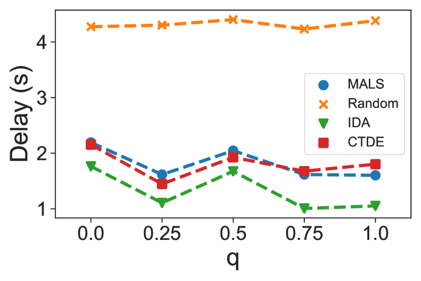
(a) Downlink delay with 4 UEs.

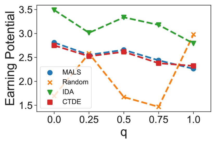
(b) Earning potential with 4 UEs.

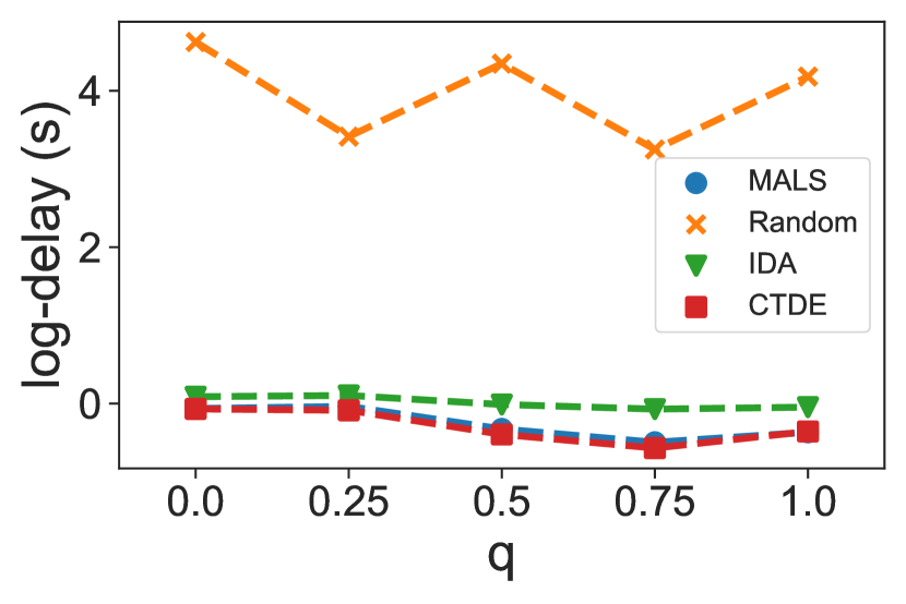
(c) Up-link delay with 4 UEs.

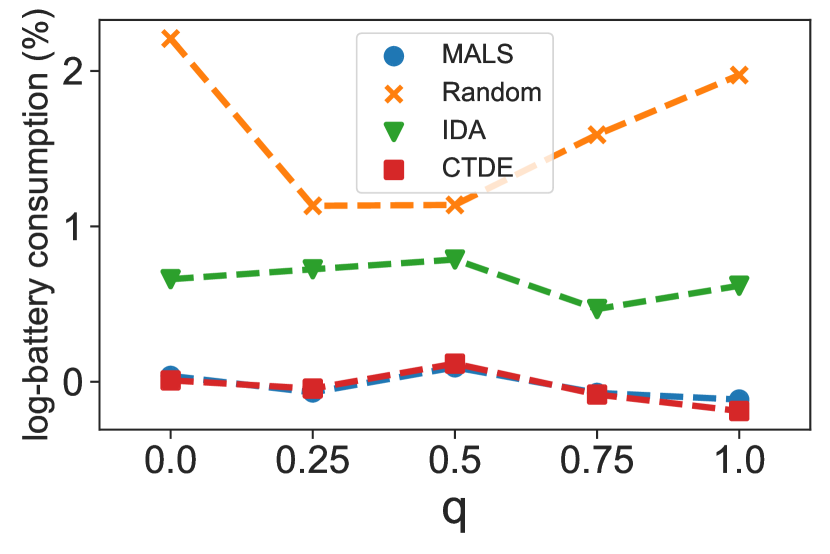
(d) Battery usage with 4 UEs.

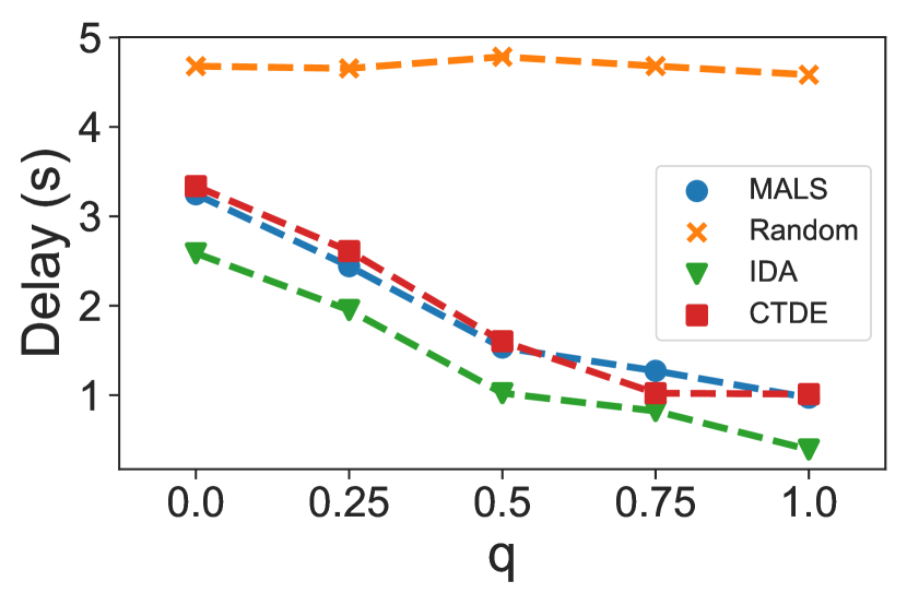
(e) Downlink delay with 5 UEs.

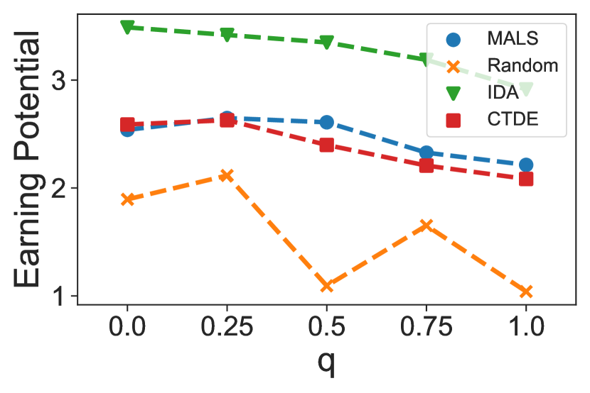
(f) Earning potential with 5 UEs.

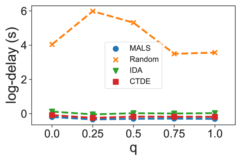
(g) Up-link delay with 5 UEs.

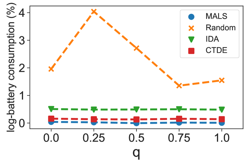
(h) Battery usage with 5 UEs.

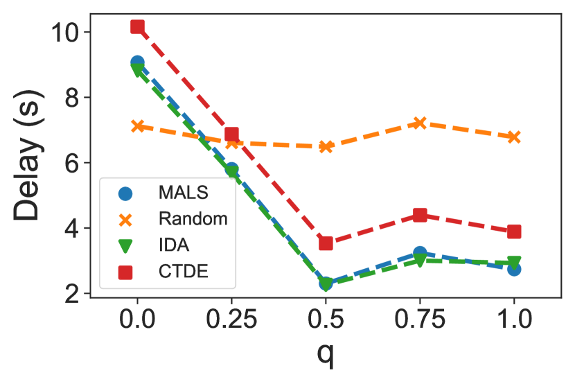
(i) Downlink delay with 6 UEs.

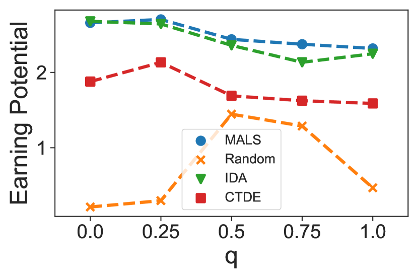
(j) Earning potential with 6 UEs.

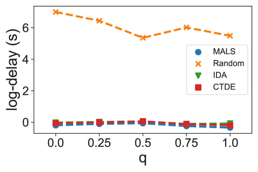
(k) Up-link delay with 6 UEs.

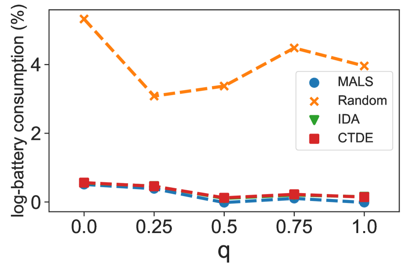
(l) Battery usage with 6 UEs.

Figure 6: Complete results - Metric values across different $q$ values.

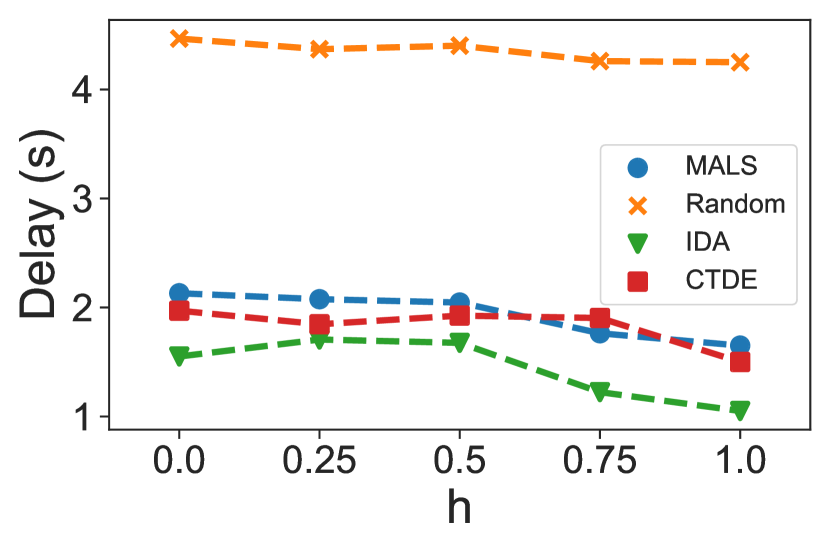
(a) Downlink delay with 4 UEs.

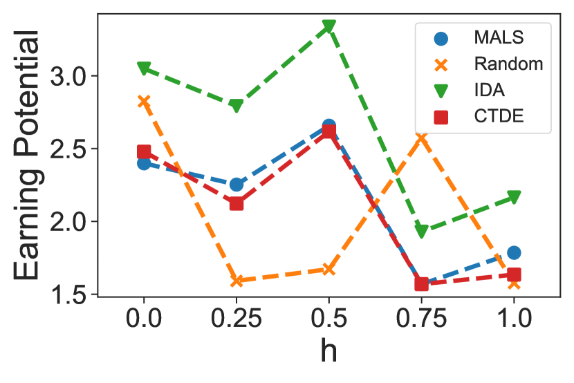
(b) Earning potential with 4 UEs.

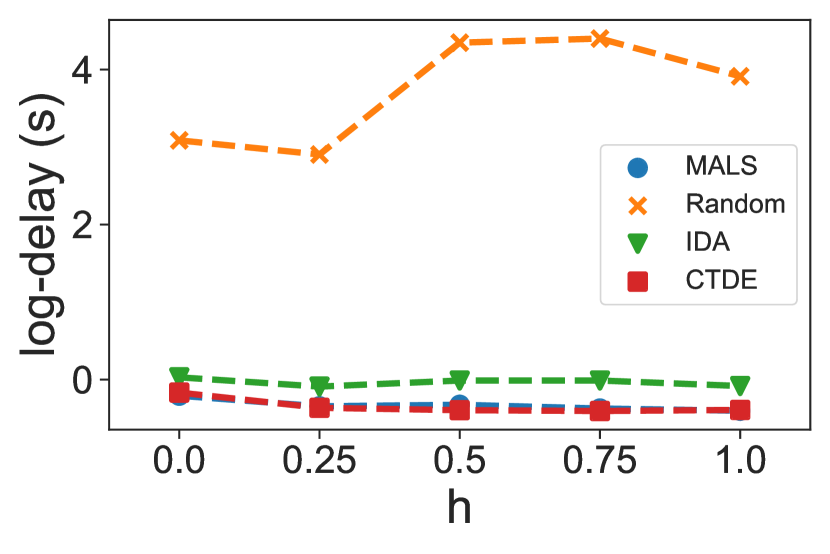
(c) Up-link delay with 4 UEs.

(d) Battery usage with 4 UEs.

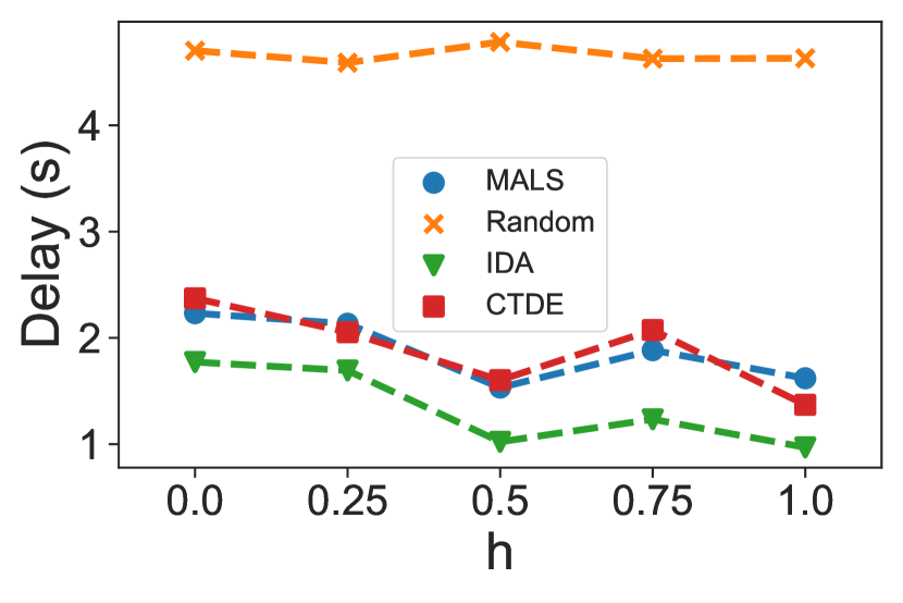
(e) Downlink delay with 5 UEs.

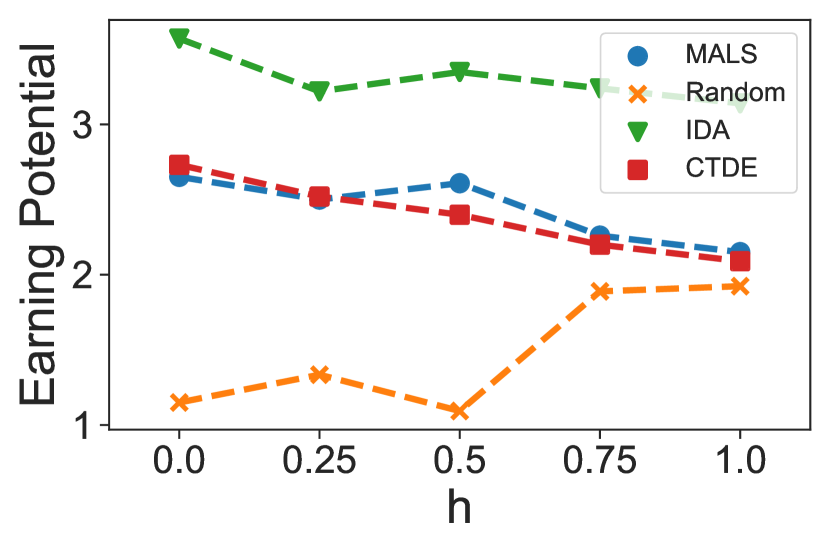
(f) Earning potential with 5 UEs.

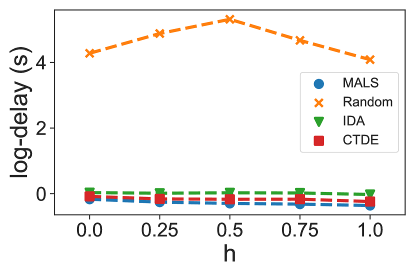
(g) Up-link delay with 5 UEs.

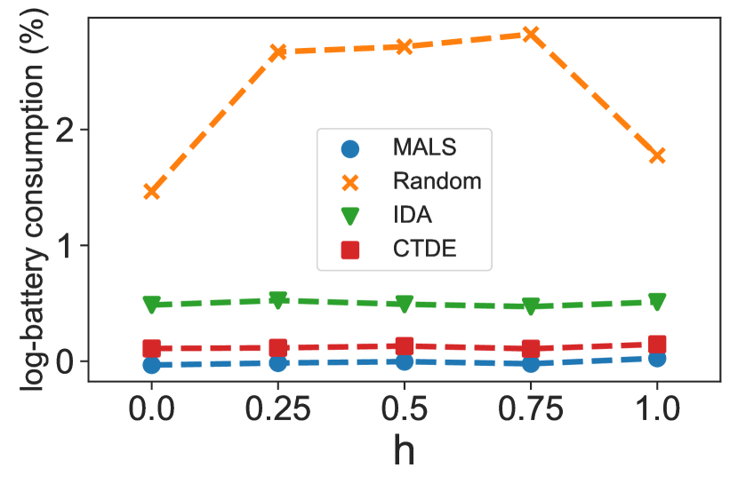
(h) Battery usage with 5 UEs.

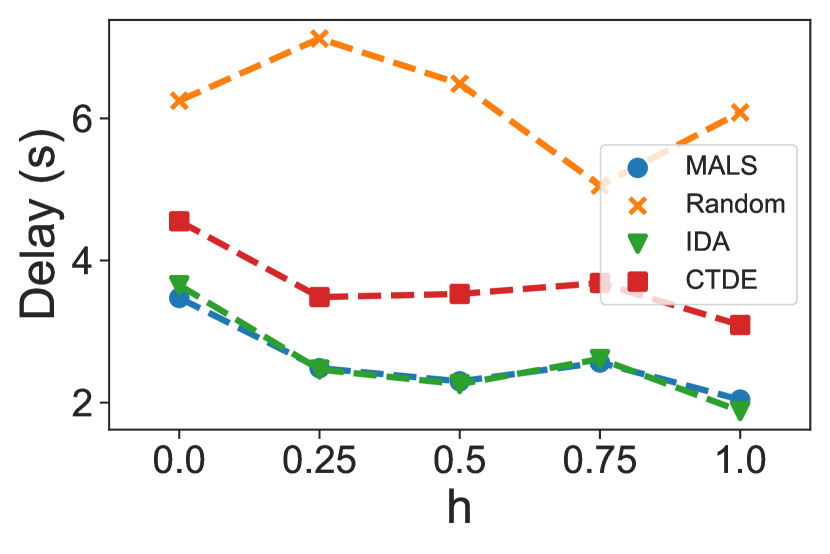
(i) Downlink delay with 6 UEs.

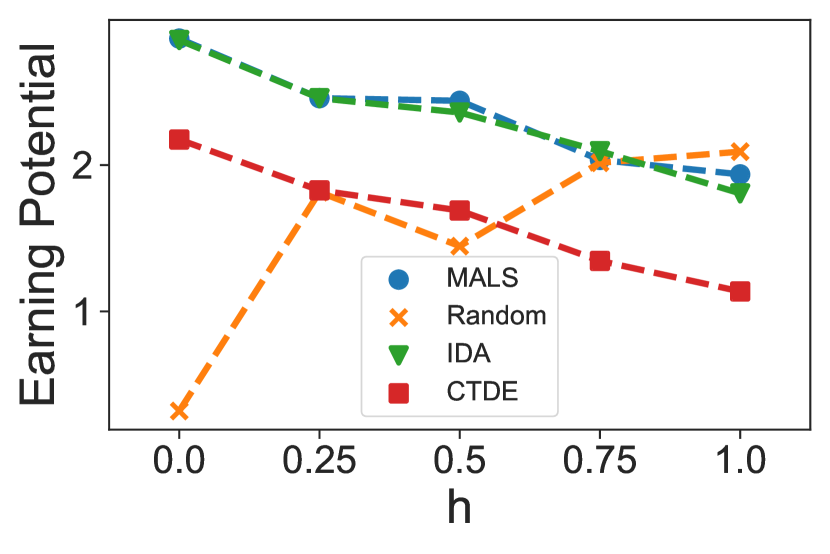
(j) Earning potential with 6 UEs.

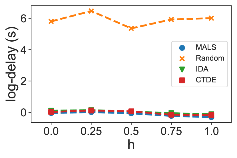
(k) Up-link delay with 6 UEs.

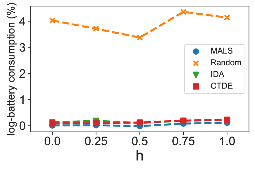
(l) Battery usage with 6 UEs.

Figure 7: Complete results - Metric values across different $h$ values.

Fig. 6 and 7 on the next page show how the performance metrics (downlink delay, worst-case (lowest) earning potential, uplink delay and worst-case (greatest) UE battery charge expenditure) vary across different $q$ and $h$ values. The changes in $q$ and $h$ corresponds to changing weight emphasis between variables downlink latency and resolution-influenced earning potential, and uplink transmission latency and worst-case (greatest) UE battery charge expenditure, respectively. Value of $h$ is $0.5$ when $q$ is varying, and vice versa.

References

- [1] T. J. Chua, W. Yu, and J. Zhao, “Play to earn in the Metaverse over wireless networks with deep reinforcement learning,” submitted to the 2023 IEEE International Conference on Communications (ICC). [Online]. Available: https://personal.ntu.edu.sg/JunZhao/ICC2023MALS.pdf
- [2] E. Sheridan, M. Ng, L. Czura, A. Steiger, A. Vegliante, and K. Campagna, “Framing the future of web 3.0: Metaverse edition,” https://www.goldmansachs.com/insights/pages/framing-the-future-of-web-3.0-metaverse-edition.html, 2021.
- [3] R. Browne, “Cash grab or innovation? the video game world is divided over NFTs,” Dec 2021. [Online]. Available: https://www.cnbc.com/2021/12/20/cash-grab-or-innovation-the-video-game-world-is-divided-over-nfts.html
- [4] N. Roos, “Best Play-to-Earn games with NFT or crypto,” November 2022. [Online]. Available: https://www.playtoearn.online/games/
- [5] “Polka city.” [Online]. Available: https://www.polkacity.io/
- [6] “Reality clash.” [Online]. Available: https://realityclash.com/
- [7] Y. Cai, J. Llorca, A. M. Tulino, and A. F. Molisch, “Compute-and data-intensive networks: The key to the Metaverse,” arXiv preprint arXiv:2204.02001, 2022.
- [8] R. Lowe, Y. I. Wu, A. Tamar, J. Harb, O. Pieter Abbeel, and I. Mordatch, “Multi-agent actor-critic for mixed cooperative-competitive environments,” Advances in Neural Information Processing Systems, vol. 30, 2017.
- [9] T. J. Chua, W. Yu, and J. Zhao, “Resource allocation for mobile Metaverse with the Internet of Vehicles over 6G wireless communications: A deep reinforcement learning approach,” in 8th IEEE World Forum on the Internet of Things (WFIoT), 2022, also available online at https://arxiv.org/pdf/2209.13425.pdf
- [10] T. J. Chua, W. Yu, and J. Zhao, “Mobile edge adversarial detection for digital twinning to the Metaverse with deep reinforcement learning,” submitted to the 2023 IEEE International Conference on Communications (ICC). [Online]. Available: https://personal.ntu.edu.sg/JunZhao/ICC2023Adversarial.pdf
- [11] Y. Han, D. Niyato, C. Leung, C. Miao, and D. I. Kim, “A dynamic resource allocation framework for synchronizing Metaverse with IoT service and data,” in ICC 2022-IEEE International Conference on Communications. IEEE, 2022, pp. 1196–1201.
- [12] W. C. Ng, W. Y. B. Lim, J. S. Ng, Z. Xiong, D. Niyato, and C. Miao, “Unified resource allocation framework for the edge intelligence-enabled Metaverse,” in ICC 2022-IEEE International Conference on Communications. IEEE, 2022, pp. 5214–5219.
- [13] M. Xu, D. Niyato, J. Kang, Z. Xiong, C. Miao, and D. I. Kim, “Wireless edge-empowered Metaverse: A learning-based incentive mechanism for virtual reality,” in IEEE International Conference on Communications (ICC), 2022, pp. 5220–5225.
- [14] M. Chen, W. Saad, and C. Yin, “Resource management for wireless virtual reality: Machine learning meets multi-attribute utility,” in GLOBECOM 2017-2017 IEEE Global Communications Conference. IEEE, 2017, pp. 1–7.
- [15] Y. Wang, M. Chen, Z. Yang, W. Saad, T. Luo, S. Cui, and H. V. Poor, “Meta-reinforcement learning for immersive virtual reality over THz/VLC wireless networks,” in ICC 2021-IEEE International Conference on Communications. IEEE, 2021, pp. 1–6.
- [16] Q. Liu, S. Huang, J. Opadere, and T. Han, “An edge network orchestrator for mobile augmented reality,” in IEEE INFOCOM 2018-IEEE Conference on Computer Communications. IEEE, 2018, pp. 756–764.
- [17] H. Wang and J. Xie, “User preference based energy-aware mobile ar system with edge computing,” in IEEE INFOCOM 2020-IEEE Conference on Computer Communications. IEEE, 2020, pp. 1379–1388.
- [18] M. Chen, W. Saad, and C. Yin, “Virtual reality over wireless networks: Quality-of-service model and learning-based resource management,” IEEE Transactions on Communications, vol. 66, no. 11, pp. 5621–5635, 2018.
- [19] H. Lu, C. Gu, F. Luo, W. Ding, and X. Liu, “Optimization of lightweight task offloading strategy for mobile edge computing based on deep reinforcement learning,” Future Generation Computer Systems, vol. 102, pp. 847–861, 2020.
- [20] T. Alfakih, M. M. Hassan, A. Gumaei, C. Savaglio, and G. Fortino, “Task offloading and resource allocation for mobile edge computing by deep reinforcement learning based on sarsa,” IEEE Access, vol. 8, pp. 54 074–54 084, 2020.
- [21] N. C. Luong, D. T. Hoang, S. Gong, D. Niyato, P. Wang, Y.-C. Liang, and D. I. Kim, “Applications of deep reinforcement learning in communications and networking: A survey,” IEEE Communications Surveys & Tutorials, vol. 21, no. 4, pp. 3133–3174, 2019.
- [22] D. Guo, L. Tang, X. Zhang, and Y.-C. Liang, “Joint optimization of handover control and power allocation based on multi-agent deep reinforcement learning,” IEEE Transactions on Vehicular Technology, vol. 69, no. 11, pp. 13 124–13 138, 2020.
- [23] C. He, Y. Hu, Y. Chen, and B. Zeng, “Joint power allocation and channel assignment for NOMA with deep reinforcement learning,” IEEE Journal on Selected Areas in Communications, vol. 37, no. 10, pp. 2200–2210, 2019.
- [24] J. R. Pierce, An introduction to information theory: symbols, signals and noise. Courier Corporation, 2012.
- [25] J. Feng and J. Zhao, “Resource allocation for augmented reality empowered vehicular edge metaverse,” arXiv preprint arXiv:2212.01325, 2022.
- [26] D. Yang, G. Xue, X. Fang, and J. Tang, “Crowdsourcing to smartphones: Incentive mechanism design for mobile phone sensing,” in Annual International Conference on Mobile Computing and Networking (MobiCom), 2012, pp. 173–184.
- [27] J. Schulman, F. Wolski, P. Dhariwal, A. Radford, and O. Klimov, “Proximal policy optimization algorithms,” arXiv preprint arXiv:1707.06347, 2017.
- [28] R. S. Sutton, D. McAllester, S. Singh, and Y. Mansour, “Policy gradient methods for reinforcement learning with function approximation,” Advances in Neural Information Processing Systems, vol. 12, 1999.
- [29] J. Schulman, P. Moritz, S. Levine, M. Jordan, and P. Abbeel, “High-dimensional continuous control using generalized advantage estimation,” arXiv preprint arXiv:1506.02438, 2015.
- [30] K. Zhang, Z. Yang, and T. Başar, “Multi-agent reinforcement learning: A selective overview of theories and algorithms,” Handbook of Reinforcement Learning and Control, pp. 321–384, 2021.
- [31] J. Foerster, G. Farquhar, T. Afouras, N. Nardelli, and S. Whiteson, “Counterfactual multi-agent policy gradients,” in Proceedings of the AAAI conference on artificial intelligence, vol. 32, no. 1, 2018.
- [32] D. P. Kingma and J. Ba, “Adam: A method for stochastic optimization,” arXiv preprint arXiv:1412.6980, 2014.