Fast solution of incompressible flow problems with two-level pressure approximation

Abstract.

This paper develops efficient preconditioned iterative solvers for incompressible flow problems discretised by an enriched Taylor–Hood mixed approximation, in which the usual pressure space is augmented by a piecewise constant pressure to ensure local mass conservation. This enrichment process causes over-specification of the pressure when the pressure space is defined by the union of standard Taylor–Hood basis functions and piecewise constant pressure basis functions, which complicates the design and implementation of efficient solvers for the resulting linear systems. We first describe the impact of this choice of pressure space specification on the matrices involved. Next, we show how to recover effective solvers for Stokes problems, with preconditioners based on the singular pressure mass matrix, and for Oseen systems arising from linearised Navier–Stokes equations, by using a two-stage pressure convection–diffusion strategy. The codes used to generate the numerical results are available online.

1. Introduction

Reliable and efficient iterative solvers for models of steady incompressible flow emerged in the early 1990s. Strategies based on block preconditioning of the underlying matrix operators using (algebraic or geometric) multigrid components have proved to be the key to realising mesh independent convergence (and optimal complexity) without the need for tuning parameters, particularly in the context of classical mixed finite element approximation, see Elman et al. [7, chap. 9]. The focus of this contribution is on efficient solver strategies in cases where (an inf–sup) stable Taylor–Hood mixed approximation is augmented by a piecewise constant pressure in order to guarantee local conservation of mass. The augmentation leads to over-specification of the pressure solution when the pressure space is defined in the natural way via the union of Taylor–Hood pressure basis functions and basis functions for the piecewise constant pressure space, requiring a redesign of the established solver technology.

The idea of adding a piecewise constant pressure to the standard rectangular biquadratic velocity, bilinear pressure ($\hbox{\msbm Q}_{2}$–$\hbox{\msbm Q}_{1}$) approximation was originally suggested during discussion around a blackboard at a conference on finite elements in fluids held in Banff in 1980; see Gresho et al. [8]. The need for local mass conservation was motivated by competition from finite volume methods (such as the MAC scheme) in the design of effective strategies for modelling buoyancy-driven flow in the atmosphere.

The extension of the augmentation idea to Taylor–Hood ($\mathbb{P}_{2}$–$\mathbb{P}_{1}$) triangular approximation was proposed in a paper presented at a conference in Reading in 1982; see Griffiths [9]. A proof of stability of the augmented $\mathbb{P}_{2}$–$\mathbb{P}_{1}^{\ast}$ approximation on triangular meshes was constructed by Thatcher & Silvester [23] in 1987. An extended version of this manuscript included discussion of $\hbox{\msbm Q}_{2}$–$\hbox{\msbm Q}_{1}^{\ast}$ hexahedral elements [22]. A rigorous assessment of the augmentation strategy was undertaken by Boffi et al. two decades later [4]. The strategy of augmenting a continuous pressure approximation to give a locally mass-conserving strategy can also be generalised to higher-order $\hbox{\msbm Q}_{k}$–$\hbox{\msbm Q}_{k-1}$ and $\mathbb{P}_{k}$–$\mathbb{P}_{k-1}$ Taylor–Hood approximations. Inf–sup stability is assured for $k\geq 2$ in two dimensions and for $\mathbb{P}_{k}$–$\mathbb{P}_{k-1}$ with $k\geq 3$ in three dimensions; see [3, p. 506].

A closely related, yet fundamentally different Stokes approximation strategy is developed in [26]. Their idea is to stabilise the lowest-order $\mathbb{P}_{1}$–$\mathbb{P}_{0}$ approximation space defined on triangles or tetrahedra by augmenting the continuous velocity approximation by a piecewise constant approximation. The extended mixed approximation is stable but nonconforming. Note that the design of linear solvers for the resulting discrete equations is relatively straightforward. A special feature of the extended approximation is that it can be augmented by postprocessing to give a pressure-robust approximation; see [12].

More generally, such an extended Galerkin (EG) approximation can be viewed as an intermediate between continuous Galerkin (CG) and discontinuous Galerkin (DG). This interpretation of piecewise constant augmentation was originally put forward by Sun & Liu [21] and is motivated by the fact that it gives local flux conservation when modelling transport in porous media flow problems, but with fewer degrees of freedom compared to vanilla DG.

The novel contribution in this work lies in the linear algebra aspects of two-field pressure approximation. The immediate issue that needs to be dealt with is the fact that, when the pressure space is specified by the frame formed by adding usual finite element basis functions for the underlying Taylor–Hood space to basis functions for the discontinuous pressure space, the mass matrix that determines the stability of the resulting mixed approximation is singular. This aspect is noted in the context of EG approximation in [14, Remark 4.1] and is discussed in section 2. The main issue that has to be dealt with in practical flow simulation is the over-specification and associated ill-conditioning of the discrete operators that arise in the preconditioning of the linearised Navier–Stokes operator. This is the focus of the discussion in section 3. The conclusion of this study is that optimal complexity convergence rates can be recovered when using two-field pressure approximation, but only after a careful redesign of the preconditioning components.

2. Two-field pressure mass matrix

In this section we consider the Stokes problem

$$-\triangle\vec{\,u}+\nabla p =\vec{\,0} \text{ in }\Omega,$$

$$\nabla\cdot\vec{\,u} =0 \text{ in }\Omega,$$

$$\vec{\,u} =\vec{\,g} \text{ on }\partial\Omega,$$

where $\vec{\,u}$ and $p$ are the fluid velocity and pressure, respectively, and $\Omega\subset\mathbb{R}^{d}$, $d\in\{2,3\}$, is a polygonal or polyhedral domain.

Throughout this section, we assume that $\boldsymbol{V}_{h}\subset H_{0}^{1}(\Omega)^{d}$ and $Q_{h}\subset L^{2}_{0}(\Omega):=\{q\in L_{2}:\int_{\Omega}q=0\}$ are an inf–sup stable pair of finite element spaces. Then the corresponding finite element approximation problem is to find $(\vec{\,u}_{h},p_{h})\in\boldsymbol{V}_{h}\times Q_{h}$ such that

$$a(\vec{\,u}_{h},\vec{\,v}_{h})+b(\vec{\,v}_{h},p_{h}) =(\vec{\,f}_{h},\vec{\,v}_{h}) \text{ for all }\vec{\,v}_{h}\in\boldsymbol{V}_{h},$$ (1a)

$$b(\vec{\,u}_{h},q_{h}) =(g_{h},q_{h}) \text{ for all }q_{h}\in Q_{h},$$ (1b)

where $(\cdot,\cdot)$ denotes the usual $L^{2}$ inner product, right-hand side functions $\vec{\,f}_{h}$ and $g_{h}$ are associated with the specified boundary velocity ($g_{h}$ is zero for enclosed flow), and

$$a(\vec{\,u},\vec{\,v})=\int_{\Omega}\nabla\vec{\,u}:\nabla\vec{\,v},\qquad b(\vec{\,u},p)=-\int_{\Omega}p\,\nabla\cdot\vec{\,u}.$$

Solving the finite element problem (1) is then equivalent to solving the linear system

$$\underbrace{\begin{bmatrix}\boldsymbol{A}&B^{T}\\ B&0\end{bmatrix}}_{\mathcal{A}}\begin{bmatrix}\boldsymbol{u}\\ \boldsymbol{p}\end{bmatrix}=\begin{bmatrix}\boldsymbol{f}\\ \boldsymbol{g}\end{bmatrix},$$ (2)

where $\boldsymbol{A}\in\mathbb{R}^{n_{u}\times n_{u}}$ is symmetric positive definite and $B\in\mathbb{R}^{n_{p}\times n_{u}}$ [7, chap. 3]. The matrix $\mathcal{A}$ is of well-known saddle point type, and solvers for this sort of system have been extensively studied, see, e.g., Benzi et al. [1]. Since $\mathcal{A}$ is large and sparse, the system is typically solved by an iterative method, with preconditioned MINRES [17] a popular choice.

An ideal preconditioner for $\mathcal{A}$ is [13, 16]

$$\mathcal{P}_{\text{ideal}}=\begin{bmatrix}\boldsymbol{A}&\\ &B\boldsymbol{A}^{-1}B^{T}\end{bmatrix},$$

since the eigenvalues of the preconditioned matrix are $0$, $1$, and $(1\pm\sqrt{5})/2$, with the zero eigenvalue appearing only if the preconditioned matrix is singular. This preconditioner is usually too costly to apply, and so efficient block diagonal preconditioners for $\mathcal{A}$ are typically based on spectrally equivalent preconditioners for $\boldsymbol{A}$ and the negative Schur complement $S=B\boldsymbol{A}^{-1}B^{T}$. For Stokes problems, the solve with $\boldsymbol{A}$ can be replaced by, e.g., an algebraic or geometric multigrid solver, while for stable discretisations $S$ is spectrally equivalent to $M_{Q}$, the pressure mass matrix [7, chap. 3], i.e., there exist constants $\gamma$ and $\Gamma$, independent of $h$, such that

$$\gamma^{2}\leq\frac{\boldsymbol{q}^{T}B\boldsymbol{A}^{-1}B^{T}\boldsymbol{q}}{\boldsymbol{q}^{T}M_{Q}\boldsymbol{q}}\leq\Gamma^{2}$$ (3)

for all vectors $\boldsymbol{q}$ except those corresponding to the function $q_{h}\equiv 1$ on $\Omega$. For certain element pairs, $M_{Q}$ itself is easily inverted, e.g., for discontinuous $\mathbb{P}_{0}$ or $\hbox{\msbm Q}_{0}$ pressures, the mass matrix is diagonal. Otherwise, $M_{Q}$ can be replaced by its diagonal or by a fixed number of steps of Chebyshev semi-iteration acceleration of a Jacobi iteration when, as is common, $\operatorname*{diag}(M_{Q})^{-1}M_{Q}$ has eigenvalues within a small interval and this interval lies away from the origin [24, 25].

To summarise, for inf–sup stable finite element pairs, an effective preconditioner for (2) is

$$\mathcal{P}=\begin{bmatrix}\boldsymbol{M}&\\ &M_{S}\end{bmatrix},$$ (4)

where $\boldsymbol{M}\in\mathbb{R}^{n_{u}\times n_{u}}$ is $\boldsymbol{A}$ or an approximation, and $M_{S}\in\mathbb{R}^{n_{p}\times n_{p}}$ is $M_{Q}$ or an approximation. (See, e.g., Elman et al. [7, chap. 4] for results with $\hbox{\msbm Q}_{2}$–$\hbox{\msbm Q}_{1}$ approximation on quadrilaterals.)

In this section, our aim is to determine effective preconditioners for the enriched Taylor–Hood element. As we will see, although enriching the pressure space results in better mass conservation properties, it can also present challenges for solving (2).

2.1. Augmented Taylor–Hood Elements

We see from (1) that the mass conservation condition $\nabla\cdot\vec{\,u}=0$ is imposed only in a weak sense, and if Taylor–Hood elements are employed we can only guarantee that (1b) will hold. However, by augmenting the pressure space by piecewise constant pressures it is possible to obtain local mass conservation, so that the average of the divergence is zero on each individual element. The natural choice is to define this space by a frame consisting of the union of the continuous Taylor–Hood pressure basis functions and the discontinuous pressure basis functions. In this case, as we will discuss later in this section, constant pressures have multiple representations, and this results in certain challenges for solving (2). Although it is certainly possible to instead compute a basis for this augmented pressure space, we show that the linear algebra challenges associated with using a frame can be overcome, which simplifies the implementation of the method.

Let us now describe the enriched Taylor–Hood finite element spaces. We first introduce a shape-regular family of simplicial, quadrilateral (in 2D) or hexahedral (in 3D) decompositions of the domain $\Omega$. We assume that any two elements have at most a common face, edge, or vertex and denote by $h$ the maximum diameter of any element. The total number of elements in the resulting mesh is $n_{el}$.

We denote the usual Taylor–Hood finite element space by $\boldsymbol{V}_{h}^{TH}\times Q_{h}^{TH}$, so that $\boldsymbol{V}_{h}^{TH}\times Q_{h}^{TH}=(\hbox{\msbm Q}_{k+1})^{d}\times\hbox{\msbm Q}_{k}$ or $\boldsymbol{V}_{h}^{TH}\times Q_{h}^{TH}=(\mathbb{P}_{k+1})^{d}\times\mathbb{P}_{k}$ with $d\geq 2$. In the latter case, we additionally assume that the polynomial degree, $k$, satisfies $k\geq d-1$. The corresponding enriched Taylor–Hood space is $\boldsymbol{V}_{h}^{TH}\times Q_{h}^{\star}$ where

$$Q_{h}^{\star} =\{q=q_{k}+q_{0},q_{k}\in Q_{h}^{TH},q_{0}\in Q_{h}^{0}\}$$ (5)

and $Q_{h}^{0}$ is the space of discontinuous pressures that are constant on each element. Thus, we see that the velocity approximation space is identical to that of the corresponding Taylor–Hood element, while $Q_{h}^{\star}$ is $Q_{h}^{TH}$ augmented with piecewise constant pressures. It follows that functions in $Q_{h}^{\star}$ may be discontinuous across inter-element boundaries.

We stress that the enriched Taylor–Hood space is well defined, and inf–sup stable. From a linear algebra perspective, however, a critical point is the representation of $Q_{h}^{\star}$. Ideally, we would like to represent functions in $Q_{h}^{\star}$ as linear combinations of basis functions. In this case the resulting linear system would be nonsingular, and it is likely that the approaches described at the stat of this section could be applied directly. However, the most natural choice is define $Q_{h}^{\star}$ by a frame, i.e., to let

$$Q_{h}^{\star}=\operatorname*{span}\{\phi_{1},\dotsc,\phi_{n_{k}},\phi_{n_{k}+1},\dotsc,\phi_{n_{p}}\},$$ (6)

where $\{\phi_{k}\}_{k=1}^{n_{k}}$ and $\{\phi_{k}\}_{k=n_{k}+1}^{n_{p}}$ are Lagrange bases of $Q_{h}^{TH}$ and $Q_{h}^{0}$ (see (5)). This approach to specifying the pressure space has been used in, e.g., [4, 19, 22].

Although this makes specification of the pressure straightforward, with this choice any constant function on $\Omega$ can be represented by a function in $Q_{h}^{TH}$ or a function in $Q_{h}^{0}$. This has profound consequences for the linear algebra: the pressure mass matrix $M_{Q}$ that determines $M_{S}$ in (4) becomes singular, and the rank of the matrix $B^{T}$ is reduced. In the rest of this section we first establish these properties, before showing that it is still possible to solve (2) by preconditioned MINRES in this case.

Using (6), we can relate vectors $\boldsymbol{p}\in\mathbb{R}^{n_{p}}$ and functions $p=p_{k}+p_{0}\in Q_{h}^{\star}$, where $p_{k}\in Q_{h}^{TH}$, $p_{0}\in Q_{h}^{0}$. Specifically,

$$p=\sum_{i=1}^{n_{p}}\boldsymbol{p}_{i}\phi_{i},\quad p_{k}=\sum_{i=1}^{n_{k}}\boldsymbol{p}_{i}\phi_{i}\quad\text{ and }\quad p_{0}=\sum_{i=n_{k}+1}^{n_{p}}\boldsymbol{p}_{i}\phi_{i}.$$ (7)

As mentioned above, any constant function has multiple representations when specified via (6). In particular, $p=p_{k}+p_{0}\equiv 0$ with $p_{k}=\alpha$ and $p_{0}=-\alpha$, for any $\alpha\in\mathbb{R}$. We see from (7) that this representation of the zero function corresponds to the vector $\alpha\boldsymbol{k}$, where

$$\boldsymbol{k}=\begin{bmatrix}\boldsymbol{1}_{n_{k}}\\ -\boldsymbol{1}_{n_{0}}\end{bmatrix}$$ (8)

and $n_{0}=n_{p}-n_{k}$. A direct consequence of the correspondence between $\boldsymbol{k}$ and the zero function on $\Omega$ is that $M_{Q}\boldsymbol{k}=\boldsymbol{0}$ and $B^{T}\boldsymbol{k}=\boldsymbol{0}$, as we now show.

Proposition 1.

Let

$$M_{Q}=[q_{ij}]_{i,j=1}^{n_{p}},\quad q_{ij}=\int_{\Omega}\phi_{i}\phi_{j},$$

be the pressure mass matrix for the enriched Taylor–Hood pressure space $Q_{h}^{\star}$ in (5), specified by the frame (6). Then, $\operatorname*{null}(M_{Q})=\operatorname*{span}\{\boldsymbol{k}\}$, where $\boldsymbol{k}$ is given in (8).

Proof.

Let $\boldsymbol{p}\in\mathbb{R}^{n_{p}}$, $\boldsymbol{p}\neq\boldsymbol{0}$. Then, using (7), we find that

$$M_{Q}\boldsymbol{p}=0\quad\Leftrightarrow\quad\boldsymbol{p}^{T}M_{Q}\boldsymbol{p}=0\quad\Leftrightarrow\quad\int_{\Omega}\left(\sum_{i=1}^{n_{p}}\boldsymbol{p}_{i}\phi_{i}\right)\left(\sum_{j=1}^{n_{p}}\boldsymbol{p}_{j}\phi_{j}\right)=0\Leftrightarrow\quad\int_{\Omega}p^{2}=0,$$

which implies that $p\equiv 0$ in $\Omega$ since $p$ is continuous on each element. Since $p\equiv 0$ corresponds to vectors of the form $\alpha\boldsymbol{k}$, we find that $\operatorname*{span}\{\boldsymbol{k}\}\subseteq\operatorname*{null}(M_{Q})$.

We now show that there are no other vectors in the nullspace. Since $p=p_{k}+p_{0}\equiv 0$, $p_{k}\in Q_{h}^{TH}$, $p_{0}\in Q_{h}^{0}$, we must have $p_{k}=-p_{0}$ everywhere in $\Omega$. But $p_{0}$ is piecewise constant, and $p_{k}$ is continuous on $\overline{\Omega}$. It follows that $p_{0}\equiv\alpha$ and $p_{k}\equiv-\alpha$ on $\Omega$ for some constant $\alpha\in\mathbb{R}$. Such functions correspond to vectors of the form $\alpha\boldsymbol{k}$, which shows that $\operatorname*{null}(M_{Q})=\operatorname*{span}\{\boldsymbol{k}\}$, as required. ∎

Remark 2.

A very similar argument shows that $\boldsymbol{k}\in\operatorname*{null}(B^{T})$.

What do these results mean for the solution of (2) by preconditioned MINRES, when the coefficient matrix is constructed using the frame in (6)? First, if $B^{T}\boldsymbol{k}=\boldsymbol{0}$ then it follows that $\mathcal{A}$ is always singular, with $\mathcal{A}\boldsymbol{w}=\boldsymbol{0}$, where

$$\boldsymbol{w}=\begin{bmatrix}\boldsymbol{0}_{n_{u}}\\ \boldsymbol{k}\end{bmatrix}.$$ (9)

If the linear system (2) is consistent then this does not pose a problem for preconditioned MINRES. However, as we shall now see, the proposed block diagonal preconditioner (4), with $M_{S}=M_{Q}$, is also singular, and so effective preconditioning requires some care.

Algorithm 3.

Preconditioned MINRES algorithm for solving $\mathcal{A}\boldsymbol{x}=\boldsymbol{b}$ with symmetric positive definite preconditioner $\mathcal{P}$ [7, Algorithm 4.1].

1:$\boldsymbol{v}^{(0)}=\boldsymbol{0}$, $\boldsymbol{w}^{(0)}=\boldsymbol{0}$, $\boldsymbol{w}^{(1)}=\boldsymbol{0}$, $\gamma_{0}=0$

2:Choose $\boldsymbol{x}^{(0)}$, compute $\boldsymbol{v}^{(1)}=\boldsymbol{b}-\mathcal{A}\boldsymbol{x}^{(0)}$

3:Solve $\mathcal{P}\boldsymbol{z}^{(1)}=\boldsymbol{v}^{(1)}$, set $\gamma_{1}=\sqrt{\langle\boldsymbol{z}^{(1)},\boldsymbol{v}^{(1)}\rangle}$

4:Set $\eta=\gamma_{1}$, $s_{0}=s_{1}=0$, $c_{0}=c_{1}=1$

5:for $j=1$ until convergence do

6:     $\boldsymbol{z}^{(j)}=\boldsymbol{z}^{(j)}/\gamma_{j}$

7:     $\delta_{j}=\langle A\boldsymbol{z}^{(j)},\boldsymbol{z}^{(j)}\rangle$

8:     $\boldsymbol{v}^{(j+1)}=\mathcal{A}\boldsymbol{z}^{(j)}-(\delta_{j}/\gamma_{j})\boldsymbol{v}^{(j)}-(\gamma_{j}/\gamma_{j-1})\boldsymbol{v}^{(j-1)}$

9:     Solve $\mathcal{P}\boldsymbol{z}^{(j+1)}=\boldsymbol{v}^{(j+1)}$

10:     $\gamma_{j+1}=\sqrt{\langle\boldsymbol{z}^{(j+1)},\boldsymbol{v}^{(j+1)}\rangle}$

11:     $\alpha_{0}=c_{j}\delta_{j}-c_{j-1}s_{j}\gamma_{j}$

12:     $\alpha_{1}=\sqrt{\alpha_{0}^{2}+\gamma_{j+1}^{2}}$

13:     $\alpha_{2}=s_{j}\delta_{j}+c_{j-1}c_{j}\gamma_{j}$

14:     $\alpha_{3}=s_{j-1}\gamma_{j}$

15:     $c_{j+1}=\alpha_{0}/\alpha_{1}$; $s_{j+1}=\gamma_{j+1}/\alpha_{1}$

16:     $\boldsymbol{w}^{(j+1)}=(\boldsymbol{z}^{(j)}-\alpha_{3}\boldsymbol{w}^{(j-1)}-\alpha_{2}\boldsymbol{w}^{(j)})/\alpha_{1}$

17:     $\boldsymbol{x}^{(j)}=\boldsymbol{x}^{(j-1)}+c_{j+1}\eta\boldsymbol{w}^{(j+1)}$

18:     $\eta=-s_{j+1}\eta$

19:     <Test for convergence>

20:end for

2.2. Preconditioning considerations

Knowing that the enriched Taylor–Hood element is inf–sup stable implies that the preconditioner (4) will be effective when solving (2). However, with the common choice of frame (6), the matrix $M_{Q}$, and hence the preconditioner $\mathcal{P}$, are singular, since $\mathcal{P}\boldsymbol{w}=\boldsymbol{0}$, where $\boldsymbol{w}$ is given in (9). (Note that this implies that $\mathcal{A}$ and $\mathcal{P}$ have a common nullspace.) Here, we will show that using a singular preconditioner causes no difficulty for the preconditioned MINRES method in Algorithm 3 in exact arithmetic. At the end of section 2, we present numerical results with two different preconditioners to demonstrate our approach.

We start by noting that at each iteration step we need to solve a linear system of the form $\mathcal{P}\boldsymbol{z}^{(j)}=\boldsymbol{v}^{(j)}$. If this system is consistent there are infinitely many solutions, which take the form $\boldsymbol{z}^{(j)}=\overline{\boldsymbol{z}}^{(j)}+\zeta_{j}\boldsymbol{w}$, with $\overline{\boldsymbol{z}}^{(j)}\perp\boldsymbol{w}$ and $\zeta_{j}\in\mathbb{R}$. Our next step is to examine the effect of $|\zeta_{j}|$ on the scalars and vectors in Algorithm 3. Observe that if the linear system $\mathcal{A}\boldsymbol{x}=\boldsymbol{b}$ is consistent then $\boldsymbol{b}\perp\boldsymbol{w}$ and so $\boldsymbol{v}^{(1)}\perp\boldsymbol{w}$. It then follows by induction that $\boldsymbol{v}^{(j)}\perp\boldsymbol{w}$, $j=1,2,\dotsc$, and that the systems $\mathcal{P}\boldsymbol{z}^{(j)}=\boldsymbol{v}^{(j)}$ are all consistent. Furthermore, $\gamma_{j}=\langle\boldsymbol{z}^{(j)},\boldsymbol{v}^{(j)}\rangle^{\frac{1}{2}}=\langle\overline{\boldsymbol{z}}^{(j)},\boldsymbol{v}^{(j)}\rangle^{\frac{1}{2}}$ because of the orthogonality of $\boldsymbol{v}^{(j)}$ and $\boldsymbol{w}$, so that $\zeta_{j}$ does not affect $\gamma_{j}$. Similarly, $\delta_{j}=\langle\mathcal{A}\boldsymbol{z}^{(j)},\boldsymbol{z}^{(j)}\rangle=\langle\mathcal{A}\overline{\boldsymbol{z}}^{(j)},\overline{\boldsymbol{z}}^{(j)}\rangle$, which shows that $\delta_{j}$ is similarly unaffected by $\zeta_{j}$. Indeed, the only quantities that are affected by the nullspace components $\zeta_{j}\boldsymbol{w}$, $j=1,2,\dotsc$, are the vectors $\boldsymbol{w}^{(j)}$ and $\boldsymbol{x}^{(j)}$. In exact arithmetic, this is not a problem, since solutions of $\mathcal{A}\boldsymbol{x}=\boldsymbol{b}$ may certainly contain a component in the direction of $\boldsymbol{w}$. However, in unlucky cases, the size of the nullspace component of $\boldsymbol{x}^{(j)}$ may be so large as to dominate the approximate solution. Alternatively, in finite precision $\boldsymbol{v}^{(j)}$ and $\boldsymbol{w}$ may not be exactly orthogonal. Hence, it may be wise to explicitly ensure that $\boldsymbol{z}\perp\boldsymbol{w}$. One option is to orthogonalise $\boldsymbol{z}$ against $\boldsymbol{w}$ after each preconditioner solve, but if $|\zeta_{j}|$ is large then the result may be inaccurate. A more robust approach is to note that solutions of $\mathcal{P}\boldsymbol{z}=\boldsymbol{r}$ are minimisers of the quadratic form

$$\frac{1}{2}\boldsymbol{z}^{T}\mathcal{P}\boldsymbol{z}-\boldsymbol{z}^{T}\boldsymbol{r},$$

since $\mathcal{P}$ is positive semidefinite. Constraining $\boldsymbol{z}$ to be orthogonal to $\boldsymbol{w}$ is then equivalent to the following optimisation problem:

$$\min_{\boldsymbol{z}}\frac{1}{2}\boldsymbol{z}^{T}\mathcal{P}\boldsymbol{z}-\boldsymbol{z}^{T}\boldsymbol{r}\quad\text{s.t.}\quad\boldsymbol{w}^{T}\boldsymbol{z}=0.$$

Applying a Lagrange multiplier approach results in the augmented system

$$\begin{bmatrix}\mathcal{P}&\boldsymbol{w}\\ \boldsymbol{w}^{T}&0\end{bmatrix}\begin{bmatrix}\boldsymbol{z}\\ \lambda\end{bmatrix}=\begin{bmatrix}\boldsymbol{r}\\ 0\end{bmatrix},$$

where $\lambda$ is the Lagrange multiplier, and solving this augmented system gives a vector $\boldsymbol{z}$ that is orthogonal to $\boldsymbol{w}$. Moreover, since

$$\begin{bmatrix}\mathcal{P}&\boldsymbol{w}\\ \boldsymbol{w}^{T}&0\end{bmatrix}=\begin{bmatrix}\boldsymbol{M}&0&0\\ 0&M_{S}&\boldsymbol{k}\\ 0&\boldsymbol{k}^{T}&0\end{bmatrix}$$

we see that only the solve with $M_{S}$ needs to be modified.

2.3. Approximating the two-level pressure mass matrix

Now let us consider approximations of the matrix $M_{Q}$ which, because of the two-level pressure approximation, has $2\times 2$ block structure:

$$M_{Q}=\begin{bmatrix}Q_{k}&R^{T}\\ R&Q_{0}\end{bmatrix},$$

where

$$Q_{k} =[q_{k,ij}],\,i,j=1,\dotsc,n_{k}, \qquad q_{k,ij} =\int_{\Omega}\phi_{j}\,\phi_{i},$$

$$R =[r_{ij}],\,i=n_{k}+1,\dotsc,n_{p},\,j=1,\dotsc,n_{k}, \qquad r_{ij} =\int_{\Omega}\phi_{j}\,\phi_{i},$$

$$Q_{0} =[q_{0,ij}],\,i,j=n_{k}+1,\dotsc,n_{p}, \qquad q_{0,ij} =\int_{\Omega}\phi_{j}\,\phi_{i}.$$

Note that $Q_{k}$ is the standard Taylor–Hood pressure mass matrix, and $Q_{0}$ is the standard discontinuous pressure mass matrix, while $R$ represents cross terms between the spaces $Q_{h}^{TH}$ and $Q_{h}^{0}$ (see (5)).

Naively, one may wish to approximate $Q_{k}$ by its diagonal, but this results in slow convergence rates; it can be shown, using the method described by Wathen [25], that $\operatorname*{diag}(Q_{k})^{-1}Q_{k}$ has eigenvalues in an interval $[0,\mu]$ where, for example, for $\mathbb{P}_{1}$ elements on triangles $\mu=3$. Accordingly, applying a fixed number of iterations of a Chebyshev semi-iteration based on a Jacobi iteration, as is standard for nonsingular Galerkin mass matrices [24], leads to large iteration counts here. Replacing $Q_{k}$ or $Q_{0}$ in $M_{Q}$ by their diagonals results in similarly poor performance.

However, it is possible to replace $M_{Q}$ by an approximation designed for symmetric positive semidefinite matrices, see, e.g., [5, 6, 15] and the references therein. For example, symmetric Gauss–Seidel is convergent for such matrices [6]. Here, we have applied a fixed number of iterations of Chebyshev semi-iteration based on symmetric Gauss–Seidel [5]. The results are still mesh-dependent, because the largest non-unit eigenvalue of the underlying symmetric Gauss–Seidel iteration matrix approaches 1 as the mesh is refined but, for large problems, the cost per iteration is much lower than applying $M_{Q}$ exactly.

2.4. Reliable computation of the discrete inf–sup constant

The inf–sup constant depends on the shape of the domain $\Omega$. Thus the constant for a step domain with a long channel is much smaller than the constant for a square domain. Estimation of the inf–sup constant dynamically provides useful information regarding the connection between the velocity error and the pressure error. The inf–sup constant also features in the norm equivalence between the residual norm of the saddle-point system and the natural “energy” norm $\|\nabla u\|_{L^{2}(\Omega)}+\|p\|_{L^{2}_{0}(\Omega)},$ as discussed in the motivating paper [20].

A typical strategy to estimate the inf–sup constant for (1) is to find the largest $\gamma$ that satisfies (3), i.e., to find the smallest nonzero eigenvalue of the generalised eigenvalue problem

$$B\boldsymbol{A}^{-1}B^{T}\boldsymbol{v}=\lambda M_{Q}\boldsymbol{v},$$ (10)

where $\boldsymbol{A}$ is prescribed by the velocity basis functions, $M_{Q}$ by the pressure functions, and $B$ by both the velocity and pressure functions.

Although the inf–sup constant is independent of the choice of these functions, in practice, its computation may be affected. For example, with the common choice to define $Q_{h}^{\star}$ by the frame (6), Proposition 1 and Remark 2 show that $\boldsymbol{k}$ lies in the nullspaces of both $B^{T}$ and $M_{Q}$, which means that this generalised eigenvalue problem is singular, i.e., any $\lambda\in\mathbb{R}$ satisfies (10) when $\boldsymbol{v}=\boldsymbol{k}$. It is known that generalised eigenvalue problems with singular pencils are challenging to solve numerically [10], and additional checks must be performed to ensure that an estimate of $\gamma$ is not associated with the eigenvector $\boldsymbol{k}$. In practice we find that standard methods for computing eigenvalues of sparse matrices may struggle to accurately compute these eigenvalues, precisely because $B\boldsymbol{A}^{-1}B^{T}$ and $M_{Q}$ are singular.

An alternative is to define $Q_{h}^{\star}$ by a basis instead of the commonly-used frame (6), but it turns out that this is not necessary. The EST-MINRES approach proposed in [20] is much more robust for this singular eigenvalue problem and gives consistently reliable results for certain preconditioners. The intuition is that by ensuring that any solves with $M_{Q}$ are orthogonal to $\boldsymbol{k}$ within the preconditioned MINRES method, (see Section 2.2), we instead solve (10) for $\boldsymbol{v}\perp\boldsymbol{k}$.

We illustrate the EST-MINRES inf–sup constant estimates using two representative test problems that we describe below. All numerical results were obtained using T-IFISS [2] (for triangular elements) and IFISS3D [18] (for cubic elements). The stopping criterion for preconditioned MINRES is a reduction of the norm of the preconditioned residual by eight orders of magnitude, i.e., $\|\boldsymbol{r}_{k}\|_{\mathcal{P}^{-1}}/\|\boldsymbol{r}_{0}\|_{\mathcal{P}^{-1}}<10^{-8}$. We apply two different block diagonal preconditioners (4). The first is

$$\mathcal{P}_{1}=\begin{bmatrix}\boldsymbol{A}&\\ &M_{Q}\end{bmatrix}.$$

Although this preconditioner is expensive to apply, because it involves exact solves with $\boldsymbol{A}$, we have used it here to more clearly illustrate the key findings of this section, namely, that (4) with $M_{S}=M_{Q}$ is an effective preconditioner for augmented Taylor–Hood problems, despite the singularity of $M_{Q}$, and that EST-MINRES provides reliable approximations to $\gamma$, the discrete inf–sup constant in (3). However, we note that it is possible to replace $\boldsymbol{A}$ by, e.g., an algebraic multigrid method such as the HSL code MI20 [11]. With this AMG approximation, we are able to solve a 3D problem with nearly $10^{6}$ degrees of freedom in under 10 seconds on a quad-core, 62 GB RAM, Intel i7-6700 CPU with 3.20GHz. Moreover, the effect on the inf–sup constant is fairly small.

Our second, cheaper, preconditioner is

$$\mathcal{P}_{2}=\begin{bmatrix}\boldsymbol{A}_{\text{AMG}}&\\ &M_{\text{cheb}}\end{bmatrix},$$

where $\boldsymbol{A}_{\text{AMG}}$ is one AMG V-cycle, with the default parameters in T-IFISS and IFISS3D and $M_{\text{cheb}}$ is 20 iterations of a Chebyshev semi-iteration method based on symmetric Gauss–Seidel.

Test problem 1 (two-dimensional enclosed flow).

Our first example is a classical driven-cavity flow in the square domain $D=[-1,1]^{2}$. A Dirichlet no-flow condition is imposed on the bottom and side boundaries, while on the lid the nonzero tangential velocity is $u_{y}=1-x^{4}$. The domain is subdivided uniformly into $n^{2}$ bisected squares. We use the standard $\mathbb{P}_{2}$–$\mathbb{P}_{1}$ Taylor–Hood mixed approximation and the augmented $\mathbb{P}_{2}$–$\mathbb{P}_{1}^{\ast}$ approximation. The two components of the pressure solution for the $\mathbb{P}_{2}$–$\mathbb{P}_{1}^{\ast}$ approximation, computed for $n=32$, are illustrated in Fig. 1. The centroid pressure field is concentrated in the two corners where the pressure is singular, and the centroid pressures are an order of magnitude smaller than the vertex pressure in all elements. Consequently, the overall pressure field is visually identical to the $\mathbb{P}_{1}$ pressure field shown in the left plot in Fig. 1.

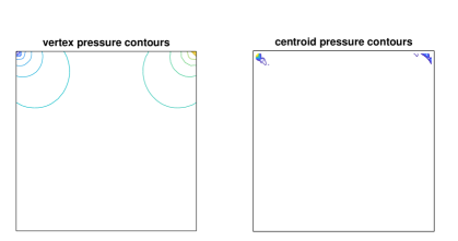
Figure 1. Representative $\mathbb{P}_{2}$–$\mathbb{P}_{1}^{*}$ pressure field solution for the cavity flow in Example 1 computed on a uniform mesh with 2048 right-angled triangles and 1089 vertices.

Test problem 2 (three-dimensional enclosed flow).

Our second problem is a three-dimensional version of driven-cavity flow. The domain is now $D=[-1,1]^{3}$. As in the previous example, the flow is enclosed, but now the nonzero tangential velocity $u_{y}=(1-x^{4})(1-z^{4})$ is specified on the top of the cavity. The domain is subdivided uniformly into $n^{3}$ cubic elements, and we use $\hbox{\msbm Q}_{2}$–$\hbox{\msbm Q}_{1}$ and $\hbox{\msbm Q}_{2}$–$\hbox{\msbm Q}_{1}^{\ast}$ approximations.

Table 1 shows preconditioned MINRES iteration counts and EST-MINRES discrete inf–sup constant approximations for Example 1 with preconditioner $\mathcal{P}_{1}$. We first note that for both the $\mathbb{P}_{2}$–$\mathbb{P}_{1}$ and $\mathbb{P}_{2}$–$\mathbb{P}_{1}^{\ast}$ approximations the iteration counts are quite similar and are mesh independent. In both cases the inf–sup constant approximations also appear to be converging from above. The approximation for $\mathbb{P}_{2}$–$\mathbb{P}_{1}^{\ast}$ elements appears to rapidly converge to four digits, indicating that even a relatively coarse grid is sufficient to obtain an approximation to the discrete inf–sup constant. However, the approximation for $\mathbb{P}_{2}$–$\mathbb{P}_{1}$ elements appears to converge more slowly. We also note that the two approaches give different inf–sup constant estimates, at least for the grids shown here. This is not so surprising as the matrices in (3) depend on the choice of finite element spaces.

When we replace the preconditioner by the cheaper $\mathcal{P}_{2}$, the situation is largely unchanged for $\mathbb{P}_{2}$–$\mathbb{P}_{1}$ elements (see Table 2). However, for $\mathbb{P}_{2}$–$\mathbb{P}_{1}^{\ast}$ elements, the preconditioned MINRES convergence rate and inf–sup constant estimate degrade as the mesh is refined. The effect on the convergence rate is caused by the largest non-unit eigenvalue of the symmetric Gauss–Seidel iteration matrix approaching 1 as the mesh is refined; this appears to also impact inf–sup constant approximation.

Fig. 2 plots the inf–sup approximations at each iteration of preconditioned MINRES for Example 1 for preconditioner $\mathcal{P}_{1}$. We see that a good approximation of the inf–sup constant is obtained after 20–25 iterations. It is again clear that for the enriched Taylor–Hood approximations we obtain very similar approximations for all grids.

	$\mathbb{P}_{2}$–$\mathbb{P}_{1}$				$\mathbb{P}_{2}$–$\mathbb{P}_{1}^{\ast}$
Grid	Velocity dof	Pressure dof	Iters	$\gamma^{2}$	Velocity dof	Pressure dof	Iters	$\gamma^{2}$
4	2178	289	37	0.1947	2178	801	42	0.1397
5	8450	1089	37	0.1926	8450	3137	42	0.1396
6	33282	4225	39	0.1911	33282	12417	40	0.1395
7	132098	16641	37	0.1898	132098	49409	40	0.1395
8	526338	66049	37	0.1888	526338	197121	40	0.1395

Table 1. Preconditioned MINRES iterations and discrete inf–sup constant approximations for Example 1 and preconditioner $\mathcal{P}_{1}$.

	$\mathbb{P}_{2}$–$\mathbb{P}_{1}$				$\mathbb{P}_{2}$–$\mathbb{P}_{1}^{\ast}$
Grid	Velocity dof	Pressure dof	Iters	$\gamma^{2}$	Velocity dof	Pressure dof	Iters	$\gamma^{2}$
4	2178	289	42	0.1961	2178	801	59	0.1404
5	8450	1089	42	0.1940	8450	3137	59	0.1443
6	33282	4225	44	0.1925	33282	12417	117	0.0467
7	132098	16641	45	0.1917	132098	49409	152	0.0259
8	526338	66049	45	0.1912	526338	197121	197	0.0064

Table 2. Preconditioned MINRES iterations and discrete inf–sup constant approximations for Example 1 and preconditioner $\mathcal{P}_{2}$.

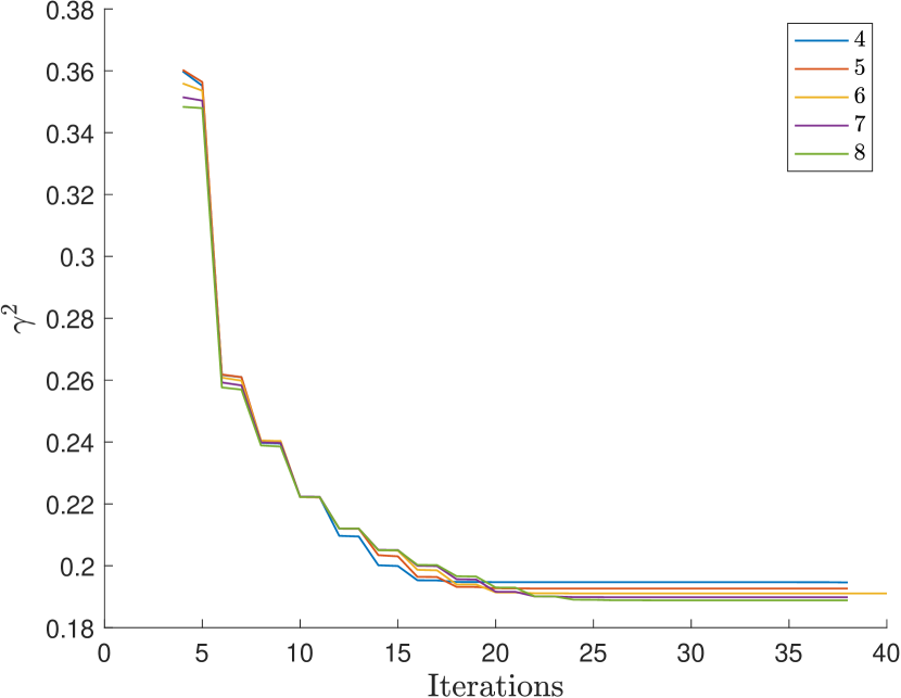
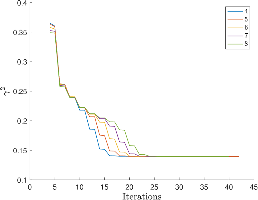
Figure 2. EST-MINRES estimates of the discrete inf–sup constant $\gamma^{2}$ at each iteration for Example 1 and preconditioner $\mathcal{P}_{1}$ with $\mathbb{P}_{2}$–$\mathbb{P}_{1}$ (left) and $\mathbb{P}_{2}$–$\mathbb{P}_{1}^{\ast}$ (right) elements for the grids specified in Table 1.

The results for Example 2 are given in Tables 3 and 4 and Fig. 3. Preconditioned MINRES iteration counts for $\mathcal{P}_{1}$ are again mesh independent and, for all but the coarsest mesh, are almost identical for the two element pairs. The discrete inf–sup constant approximations again appear to converge from above. Now, at least for the grids presented here, the estimates of $\gamma^{2}$ for Taylor–Hood elements seem to “track” the augmented Taylor–Hood estimates, i.e., the Taylor–Hood approximation on grid $j$ is almost the same as the augmented Taylor–Hood estimate on grid $j-1$. Table 4 shows that using the cheaper $\mathcal{P}_{2}$ also results in mesh-independent convergence for $\hbox{\msbm Q}_{2}$–$\hbox{\msbm Q}_{1}$ elements. Additionally, the inf–sup constant approximations seem to “track” the Taylor–Hood estimates in Table 3. Now, however, there is more modest growth in the iteration counts when this approximate preconditioner is used for $\hbox{\msbm Q}_{2}$–$\hbox{\msbm Q}_{1}^{\ast}$ elements and the inf–sup approximations are much closer to those in Table 3.

We also see from Fig. 2, which plots the inf–sup approximations at each iteration of preconditioned MINRES, for preconditioner $\mathcal{P}_{1}$, that the discrete inf–sup constant is already reasonably well approximated after 25 iterations.

	$\hbox{\msbm Q}_{2}$–$\hbox{\msbm Q}_{1}$				$\hbox{\msbm Q}_{2}$–$\hbox{\msbm Q}_{1}^{\ast}$
Grid	Velocity dof	Pressure dof	Iters	$\gamma^{2}$	Velocity dof	Pressure dof	Iters	$\gamma^{2}$
3	2187	125	45	0.1128	2187	189	48	0.1122
4	14739	729	51	0.1122	14739	1241	52	0.1115
5	107811	4913	51	0.1116	107811	9009	52	0.1110

Table 3. Preconditioned MINRES iterations and discrete inf–sup constant approximations for Example 2 and preconditioner $\mathcal{P}_{1}$.

	$\hbox{\msbm Q}_{2}$–$\hbox{\msbm Q}_{1}$				$\hbox{\msbm Q}_{2}$–$\hbox{\msbm Q}_{1}^{\ast}$
Grid	Velocity dof	Pressure dof	Iters	$\gamma^{2}$	Velocity dof	Pressure dof	Iters	$\gamma^{2}$
3	2187	125	50	0.1132	2187	189	53	0.1126
4	14739	729	54	0.1128	14739	1241	59	0.1124
5	107811	4913	56	0.1123	107811	9009	69	0.1094

Table 4. Preconditioned MINRES iterations and discrete inf–sup constant approximations for Example 2 and preconditioner $\mathcal{P}_{2}$.

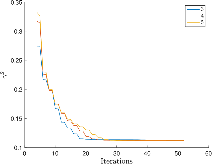
Figure 3. EST-MINRES estimates of the discrete inf–sup constant $\gamma^{2}$ at each iteration for Example 2 and preconditioner $\mathcal{P}_{1}$ with $\hbox{\msbm Q}_{2}$–$\hbox{\msbm Q}_{1}$ (left) and $\hbox{\msbm Q}_{2}$–$\hbox{\msbm Q}_{1}^{\ast}$ (right) elements for the grids specified in Table 3.

3. Two-field pressure preconditioning strategies for Oseen flow.

In this section we consider the Oseen problem

$$-\nu\triangle\vec{\,u}+\vec{\,w}\cdot\nabla\vec{\,u}+\nabla p =\vec{\,0} \text{ in }\Omega,$$

$$\nabla\cdot\vec{\,u} =0 \text{ in }\Omega,$$

$$\vec{\,u} =\vec{\,g} \text{ on }\partial\Omega,$$

that arises from applying fixed point iteration to the Navier–Stokes equations modelling steady flow in a channel domain $\Omega\subset\mathbb{R}^{2}$ with viscosity parameter $\nu$. The Oseen problem is a linear elliptic system of PDEs and assuming a divergence-free convection field $\vec{\,w}$ and a smooth (e.g., polygonal) domain $\Omega$, has a unique weak solution for all positive values of the viscosity parameter. The inf–sup stability of our two-field mixed approximation is a sufficient condition for convergence of the mixed approximation to the weak solution of the Oseen problem as $h\to 0$.

Our focus will be on the associated discrete matrix system,

$$\left[\begin{array}[]{@{}cc@{}}\boldsymbol{F}&B^{T}\\ B&0\end{array}\right]\left[\begin{array}[]{@{}c@{}}\mathbf{u}\\ \mathbf{p}\end{array}\right]=\left[\begin{array}[]{@{}c@{}}\mathbf{f}\\ \mathbf{g}\end{array}\right],$$ (17)

where the unknown coefficient vector involves the discrete velocity vector $\mathbf{u}\in\mathbb{R}^{n_{u}}$ and the two-field pressure vector $\mathbf{p}\in\mathbb{R}^{n_{p}}$. The right-hand side vectors $\mathbf{f}$ and $\mathbf{g}$ are associated with the specified boundary velocity (as in the Stokes flow case). References to the “residual norm” throughout this section will refer to the standard Euclidean norm for finite dimensional vectors. Thus, for the system (17) the convergence of our iterative solver strategies is assessed by monitoring

$$\|\mathbf{z}\|:=\left\|\left[\begin{array}[]{@{}l@{}}\mathbf{f}-\boldsymbol{F}\mathbf{u}-B^{T}\mathbf{p}\\ \mathbf{g}-B\mathbf{u}\end{array}\right]\right\|_{\ell_{2}}.$$ (20)

The nonsymmetry of the matrix $\boldsymbol{F}$ means that the iterative solver of choice is GMRES (see [7, section 9.1]) together with a block preconditioning operator of the form

$$\mathcal{M}=\left[\begin{array}[]{@{}cc@{}}\boldsymbol{M}&B^{T}\\ 0&-M_{S}\end{array}\right],$$ (23)

where $\boldsymbol{M}$ is an optimal complexity (multigrid) operator effecting the action of the inverse of the matrix $\boldsymbol{F}$ and $M_{S}$ is an optimal complexity approximation of the Schur complement matrix $B\boldsymbol{F}^{-1}B^{T}$. We will discuss results for two representative flow problems herein.

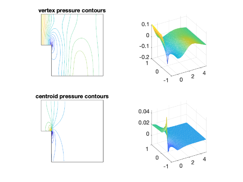
Figure 4. Representative $\mathbb{P}_{2}$–$\mathbb{P}_{1}^{*}$ pressure field solution for flow over a step ($\mathcal{R}=100$) computed on a uniform mesh with 5632 right-angled triangles and 2945 vertices.

Test problem 3 (flow over a step).

We consider an inflow–outflow problem defined on the domain $D=[-1,0)\times[0,1]\cup[0,5]\times[-1,1]$ with the viscosity parameter $\nu$ set to $1/50$ and a parabolic velocity $u_{x}=4y(1-y)$ specified on the inflow boundary $x=-1$. The construction of the standard weak formulation (see [7, p. 127]) gives rise to a natural boundary condition that fixes the hydrostatic pressure level by weakly enforcing a zero mean pressure at the outflow boundary $x=5$. (The other boundary conditions are associated with fixed walls.) We consider the discrete system (17) that results after 5 fixed-point iterations of the discretised Navier–Stokes system starting from the corresponding Stokes flow solution. We generate solutions using $\hbox{\msbm Q}_{2}$–$\hbox{\msbm Q}_{1}^{\ast}$ or $\mathbb{P}_{2}$–$\mathbb{P}_{1}^{\ast}$ augmented Taylor–Hood mixed approximation with the domain subdivided uniformly into (bisected) squares. The resulting system (17) is singular with the one-dimensional pressure nullspace described in section 2. The two components of the pressure solution computed on a representative $\mathbb{P}_{2}$–$\mathbb{P}_{1}^{\ast}$ mesh are illustrated in Fig. 4. The centroid pressure values are an order of magnitude smaller than the vertex pressure in all the elements—they provide the “corrections” to the vertex pressures that are needed to ensure local (elementwise) conservation of mass.

Test problem 4 (two-dimensional enclosed flow).

We consider the classical driven-cavity enclosed flow problem defined on the domain $D=[-1,1]^{2}$ with the viscosity parameter $\nu$ set to $1/100$ and a nonzero tangential velocity $u_{y}=1-x^{4}$ specified on the top of the cavity. We take $\mathbb{P}_{2}$–$\mathbb{P}_{1}^{\ast}$ augmented Taylor–Hood mixed approximation with the domain subdivided uniformly into $n^{2}$ bisected squares. We consider the discrete system (17) that arises after 5 fixed-point iterations starting from the corresponding Stokes flow solution. The discrete system is singular with a two-dimensional pressure nullspace, corresponding to a constant vertex pressure and a constant centroid pressure. The contour plot on the left in Fig. 5 shows the element divergence errors $\|\nabla\cdot\vec{\,u}_{h}\|_{L^{2}(\triangle)}$ computed on a coarse mesh ($n=32$). The associated centroid “correction” pressure field contours shown on the plot in the right can be seen to provide a good indication of the regions where the divergence error is concentrated. As in Fig. 4 the centroid pressure values are an order of magnitude smaller than the vertex pressure in all elements, so the overall pressure field is visually identical to the $\mathbb{P}_{1}$ pressure field (not shown here).

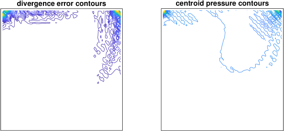
Figure 5. Comparison of divergence error and $\mathbb{P}_{2}$–$\mathbb{P}_{1}^{*}$ centroid pressure solution for cavity flow ($\mathcal{R}=200$) computed on a uniform mesh with 2048 right-angled triangles and 1089 vertices.

3.1. Pressure convection-diffusion preconditioning for Oseen flow.

There are two alternative ways of approximating the key matrix $B\boldsymbol{F}^{-1}B^{T}$ in the case that $B^{T}$ is generated by a two-field pressure approximation so that $B^{T}=[B_{1}^{T},B_{0}^{T}]$. The focus will be on pressure convection-diffusion (PCD) preconditioning in this section. Both of the Schur complement approximations can be motivated by starting with the Oseen matrix operator (17) and observing that the diagonal blocks of $\boldsymbol{F}$ are discrete representations of the convection–diffusion operator

$$\mathcal{L}=-\nu\nabla^{2}+\vec{\,w}_{h}\cdot\nabla,$$ (24)

defined on the velocity space. In practical calculations $\nu>0$ is proportional to the inverse of the flow Reynolds number and $\vec{\,w}_{h}$ is the discrete approximation to the flow velocity computed at the most recent nonlinear iteration. The PCD approximation supposes that there is an analogous operator to (24), namely

$$\mathcal{L}_{p}=(-\nu\nabla^{2}+\vec{\,w}_{h}\cdot\nabla)_{p}$$ (25)

defined on the two components of the augmented pressure space.

To this end, defining $\{\phi_{j}\}_{j=1}^{n_{1}}$ to be the basis for the $C^{0}$ pressure discretisation, we construct matrices $Q_{1}$ and $F_{1}$ so that

$$Q_{1} =[q_{1,ij}],{\quad}q_{1,ij}=\int_{\Omega}\phi_{j}\,\phi_{i}$$

$$F_{1} =[f_{1,ij}],\quad f_{1,ij}=\nu\int_{\Omega}\nabla\phi_{j}\cdot\nabla\phi_{i}+\int_{\Omega}(\vec{\,w}_{h}\cdot\nabla\phi_{j})\,\phi_{i}.$$

We then note that if the commutator with the divergence operator

$$\mathcal{E}=\nabla\cdot(-\nu\nabla^{2}+\vec{\,w}_{h}\cdot\nabla)-(-\nu\nabla^{2}+\vec{\,w}_{h}\cdot\nabla)_{p}\,\nabla\cdot$$

is small then we have the approximation

$$0\approx(Q_{1}^{-1}B_{1})\,(\boldsymbol{M}^{-1}\boldsymbol{F})-(Q_{1}^{-1}F_{1})\,(Q_{1}^{-1}B_{1})$$ (26)

where $\boldsymbol{M}$ is the diagonal of the mass matrix associated with the basis representation of the velocity space. Rearranging (26) gives the first Schur complement approximation

$$B_{1}\,\boldsymbol{F}^{-1}B^{T}\approx Q_{1}F_{1}^{-1}(B_{1}\,\boldsymbol{M}^{-1}B^{T}).$$ (27)

A discrete version of $\mathcal{L}_{p}$ for the piecewise constant pressure space can be generated by considering the jumps in pressure across inter-element boundaries; see [7, pp. 268–370]. To this end, defining $\{\varphi_{j}\}_{j=1}^{n_{0}}$ to be the (indicator function) basis for the discontinuous pressure, we construct matrices $Q_{0}$ and $F_{0}$ via

$$Q_{0} =[q_{0,ij}],{\quad}q_{0,ij}=\int_{\Omega}\varphi_{j}\,\varphi_{i}=\begin{cases}|T_{i}|&\hbox{if }i=j,\\ \;0&\hbox{otherwise},\end{cases}$$

$$F_{0} =[f_{0,ij}],\quad f_{0,ij}=\nu\sum_{T\in\mathcal{T}_{h}}\int_{T}\nabla\varphi_{j}\cdot\nabla\varphi_{i}+\sum_{T\in\mathcal{T}_{h}}\int_{T}(\vec{\,w}_{h}\cdot\nabla\varphi_{j})\,\varphi_{i}$$

and note that if the commutator with the divergence operator is small then we have

$$0\approx(Q_{0}^{-1}B_{0})\,(\boldsymbol{M}^{-1}\boldsymbol{F})-(Q_{0}^{-1}F_{0})\,(Q_{0}^{-1}B_{0}),$$ (28)

suggesting the second Schur complement approximation

$$B_{0}\,\boldsymbol{F}^{-1}B^{T}\approx Q_{0}F_{0}^{-1}(B_{0}\,\boldsymbol{M}^{-1}B^{T}).$$ (29)

Combining (27) with (29) then gives a two-field PCD approximation

$$B\boldsymbol{F}^{-1}B^{T}\approx M_{S}:=\left[\begin{array}[]{@{}cc@{}}Q_{1}&0\\ 0&Q_{0}\end{array}\right]\left[\begin{array}[]{@{}cc@{}}F_{1}^{-1}&0\\ 0&F_{0}^{-1}\end{array}\right]B\boldsymbol{M}^{-1}B^{T}.$$ (34)

Two features of the PCD approximation (34) are worth noting. The first point is that the coupling between the pressure components is represented by the $2\times 2$ block matrix $B\boldsymbol{M}^{-1}B^{T}$ rather than by the pressure mass matrix $M_{Q}$. The second key point is that the matrices $M_{S}$ and $B\boldsymbol{F}^{-1}B^{T}$ have the same nullspace, independent of the nature of underlying flow problem that is being solved.

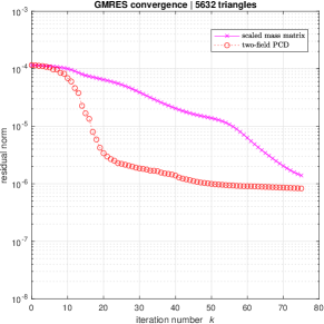
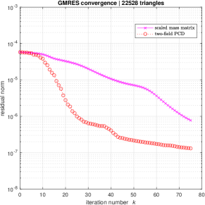
Figure 6. Absolute residual reduction for test problem 3 when computing $\mathbb{P}_{2}$–$\mathbb{P}_{1}^{*}$ solutions using preconditioners $\mathcal{M}_{1}$ (x) or $\mathcal{M}_{2}$ (o) on two nested meshes.

The PCD approximation in (34) is imperfect in practice. To illustrate this, representative convergence histories that arise in solving the inflow-outflow problem using $\mathbb{P}_{2}$–$\mathbb{P}_{1}^{*}$ approximation (shown in Fig. 4) are presented in Fig. 6. Taking the solution from the previous Picard iteration as the initial guess, we note that the initial residual norm of the target matrix system (17) is close to $10^{-4}$ independent of the spatial discretisation. Convergence plots are presented for two preconditioning strategies, namely

$$\mathcal{M}_{1}=\left[\begin{array}[]{@{}cc@{}}\boldsymbol{F}&B^{T}\\ 0&-{1\over\nu}M_{Q}\end{array}\right],\quad\mathcal{M}_{2}=\left[\begin{array}[]{@{}cc@{}}\boldsymbol{F}&B^{T}\\ 0&-M_{S}\end{array}\right],$$ (39)

with $M_{S}$ defined in (34). The first strategy is the block triangular extension of the Stokes preconditioning strategy discussed in section 2. We note that the resulting convergence is very slow—around 50 iterations are required to reduce the residual norm by an order of magnitude—but is independent of the discretisation level. In contrast we see that the PCD preconditioning strategy has two distinctive phases of convergence behaviour. An initial phase of relatively fast convergence is followed by a secondary phase where GMRES stagnates. We hypothesise that this stagnation is a consequence of the ill-conditioning of the eigenvectors of the matrix operator $M_{S}$. A notable feature is that the onset of the stagnation is delayed when solving the same problem on a finer grid. The two-phase convergence behaviour is ubiquitous—the same pattern is seen using rectangular elements and the stagnation does not go away when the viscosity parameter is increased from $1/50$ to $1/5$. An alternative strategy is clearly needed!

One way of designing a more robust PCD preconditioning strategy for a two-field pressure approximation is to exploit the fast convergence of the PCD approximation for the unaugmented Taylor-Hood approximation. The starting point for such a strategy is to rewrite the system (17) in the form

$$\left[\begin{array}[]{@{}ccc@{}}\boldsymbol{F}&B_{1}^{T}&B_{0}^{T}\\ B_{1}&0&0\\ B_{0}&0&0\end{array}\right]\left[\begin{array}[]{@{}l@{}}\mathbf{u}\\ \mathbf{p}_{1}\\ \mathbf{p}_{0}\end{array}\right]=\left[\begin{array}[]{@{}l@{}}\mathbf{f}\\ \bf{0}\\ \bf{0}\end{array}\right].$$ (49)

The proposed solution algorithm is then a two-stage process.

• Input: residual reduction tolerance $\eta$ and reduced system residual factor $c$

• Generate a PCD solution to the reduced system

  $$\left[\begin{array}[]{@{}cc@{}}\boldsymbol{F}&B_{1}^{T}\\ B_{1}&0\end{array}\right]\left[\begin{array}[]{@{}c@{}}\mathbf{u}_{1}\\ \mathbf{q}_{1}\end{array}\right]=\left[\begin{array}[]{@{}c@{}}\mathbf{f}\\ \bf{0}\end{array}\right]$$ (56)

  using the Schur complement approximation (26), stopping the GMRES iteration when the residual is reduced by a factor of $c\eta$.

• Generate a solution to the target system (49) with residual tolerance $\eta$ using preconditioning strategy $\mathcal{M}_{1}$ in (39) with the refined initial guess $[\mathbf{u}_{1}^{*},\mathbf{q}_{1}^{*},{\bf 0}]$.

• Output: refined solution $[\mathbf{u}^{*},\mathbf{p}_{1}^{*},\mathbf{p}_{0}^{*}]$

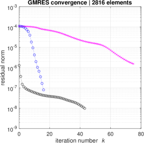
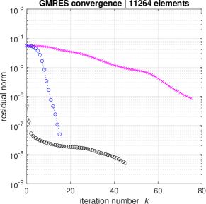
Figure 7. Absolute residual reduction for test problem 3 when computing $\hbox{\msbm Q}_{2}$–$\hbox{\msbm Q}_{1}^{*}$ solutions using using preconditioners $\mathcal{M}_{1}$ (x) or refined PCD (o) on two nested meshes.

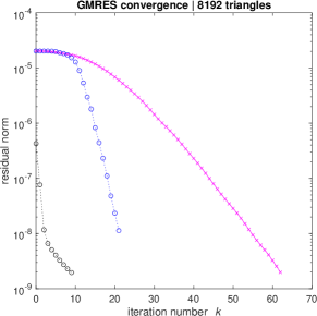
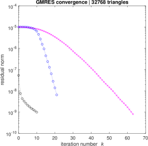
Figure 8. Absolute residual reduction for test problem 4 when computing $\mathbb{P}_{2}$–$\mathbb{P}_{1}^{*}$ solutions using using preconditioners $\mathcal{M}_{1}$ (x) or refined PCD (o) on two nested meshes.

Sample results generated using this strategy with tolerance $\eta$ set to $10^{-4}$ and $c$ set to 10 are presented in Fig. 7. Sample results for the cavity test problem are presented in Fig. 8. The results in Fig. 7 and Fig. 8 are representative of the two-stage convergence profiles that are generated when solving these test problems at other Reynolds numbers. Our experience is that the level of residual reduction is perfectly robust with regards to the spatial discretisation—typically giving smaller iteration counts when the mesh resolution is increased (a known feature of PCD preconditioning). The convergence rates of both stages of the algorithm deteriorate slowly when the Reynolds number is increased. Our strategy for terminating the first stage of the iteration is motivated by the following result.

Proposition 4.

The residual error $\|\mathbf{z}^{*}\|$ associated with the intermediate solution $[\mathbf{u}^{*}_{1},\mathbf{q}_{1}^{*},\bf{0}]$ to the discrete system (49) satisfies the bound

$$\|\mathbf{z}^{*}\|^{2} \leq c^{2}\eta^{2}\,\|\mathbf{f}\|^{2}+\|B_{0}\mathbf{u}_{1}^{*}\|^{2},$$ (57)

where $\|\mathbf{f}\|$ is the initial residual error associated with a zero initial vector.

Proof.

The vector $\mathbf{z}^{*}$ associated with the intermediate solution is the three-component vector

$$\left[\begin{array}[]{@{}l@{}}\mathbf{r}^{*}\\ \mathbf{r}_{1}^{*}\\ \mathbf{r}_{0}^{*}\end{array}\right]=\left[\begin{array}[]{@{}l@{}}\mathbf{f}\\ \bf{0}\\ \bf{0}\end{array}\right]-\left[\begin{array}[]{@{}ccc@{}}\boldsymbol{F}&B_{1}^{T}&B_{0}^{T}\\ B_{1}&0&0\\ B_{0}&0&0\end{array}\right]\left[\begin{array}[]{@{}l@{}}\mathbf{u}_{1}^{*}\\ \mathbf{q}_{1}^{*}\\ \bf{0}\end{array}\right].$$ (70)

The stopping test for solving the reduced system ensures that

$$\|\mathbf{r}^{*}\|^{2}+\|\mathbf{r}_{1}^{*}\|^{2}\leq c^{2}\eta^{2}\,\|\mathbf{f}\|^{2}.$$ (71)

Thus we have

$$\|\mathbf{z}^{*}\|^{2}=\|\mathbf{r}^{*}\|^{2}+\|\mathbf{r}_{1}^{*}\|^{2}+\|\mathbf{r}_{0}^{*}\|^{2}\leq c^{2}\eta^{2}\,\|\mathbf{f}\|^{2}+\|B_{0}\mathbf{u}_{1}^{*}\|^{2}.$$ (72)

∎

The bound (57) has two terms on the right-hand side. While the first term can be controlled by reducing $\eta$ and/or $c$, the second term measures the local incompressibility of the intermediate Taylor–Hood solution $\|B_{0}\mathbf{u}_{1}^{*}\|^{2}=\sum_{j}\big{(}\int_{T_{j}}\!\nabla\cdot{\vec{u}_{h}}^{\,*}\big{)}^{2}$, where ${\vec{u}_{h}}^{\,*}$ is the expansion of the coefficient vector $\mathbf{u}_{1}^{*}$ in the basis of the velocity approximation space. Setting $\eta=10^{-4}$ and $c=10$ we see that the second term saturates the residual error and the residual error jumps up when the switch is made from the first to the second step of the algorithm. This “transition” jump in the residual norm is clearly evident in the convergence plots. The convergence in the second step is rapid initially but eventually mirrors the rate observed for $\mathcal{M}_{1}$ approximation with a standard starting guess.

3.2. Least square commutator approximation for Oseen flow

A second way of approximating the key matrix $B\boldsymbol{F}^{-1}B^{T}$ in the case that $B^{T}$ is generated by a two-field pressure approximation is given by the least-squares commutator (LSC) preconditioner

$$B\boldsymbol{F}^{-1}B^{T}\approx M_{S}=(B\boldsymbol{H}^{-1}B^{T})\,(B\boldsymbol{M}^{-1}\boldsymbol{F}\boldsymbol{H}^{-1}B^{T})^{-1}\,(B\boldsymbol{M}^{-1}B^{T}).$$ (73)

The attractive feature of LSC is that the construction of $M_{S}$ is completely algebraic. The only technical issue is the need to make adjustments on rows and columns associated with tangential velocity degree of freedom adjacent to inflow and fixed wall boundaries. These adjustments are associated with a diagonal scaling matrix $\boldsymbol{D}$ so that $\boldsymbol{H}=\boldsymbol{D}^{-1/2}\boldsymbol{M}\boldsymbol{D}^{-1/2}$. Full details can be found in [7, pp. 376–379]).

The LSC approximation (73) is also far from perfect when using triangular elements. To illustrate this, representative convergence histories that arise in solving the inflow-outflow problem using $\mathbb{P}_{2}$–$\mathbb{P}_{1}^{*}$ approximation are presented in Fig. 9. Convergence plots are presented for two preconditioning strategies, namely the refined PCD from the previous section and

$$\mathcal{M}_{3}=\left[\begin{array}[]{@{}cc@{}}\boldsymbol{F}&B^{T}\\ 0&-M_{S}\end{array}\right],$$ (76)

with $M_{S}$ defined in (73).

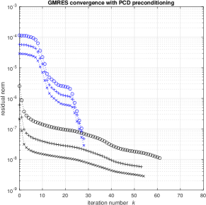
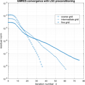
Figure 9. Absolute residual reduction for test problem 3 when computing $\mathbb{P}_{2}$–$\mathbb{P}_{1}^{*}$ solutions using using refined PCD (left) or preconditioner $\mathcal{M}_{3}$ (right) on three nested meshes.

The PCD histories in Fig. 9 display mesh independent convergence and are comparable with those observed using square elements in Fig. 7. The associated cpu times for the solution on the intermediate grid with $2\times 11264$ elements were 13 seconds for the first step (28 iterations) and 26 seconds for the second step (53 iterations). The LSC preconditioning strategy is not robust—the convergence rate deteriorates with increasing grid refinement. The cpu time for generating the LSC solution on the intermediate grid was over 100 seconds (61 iterations).

4. Conclusions

Two-level pressure approximation for incompressible flow problems offer the prospect of accurate approximation with minimal computational overhead. Derived quantities of practical importance such as the mean wall shear stress are likely to be computed much more precisely if incompressibility is enforced locally. However, the augmented pressure space causes some challenges for the linear algebra when the pressure space is defined by combining the usual Taylor–Hood pressure basis functions with basis functions for the piecewise continuous pressure space. This is because constant functions can be expressed using either the usual (continuous) Taylor–Hood pressure space, or the augmented piecewise constant pressure space. Specifically, with this common choice for specifying the pressure space, the pressure mass matrix becomes singular, and care should be taken to carefully construct and apply preconditioners that involve this matrix. Care should also be exercised when approximating the discrete inf–sup constant, and we find that naive approaches are not always reliable. On the other hand, the approximation implemented in EST-MINRES is robust. Our computational experimentation indicates that our two-stage PCD strategy could be the best way of iteratively solving two-level pressure discrete linear algebra systems in the sense of algorithmic reliability and computational efficiency.

References

- [1] M. Benzi, G. H. Golub, and J. Liesen, Numerical solution of saddle point problems, Acta Numer., 14 (2005), pp. 1–137.
- [2] A. Bespalov, L. Rocchi, and D. Silvester, T–IFISS: a toolbox for adaptive FEM computation, Comput. Math. Appl., 81 (2021), pp. 373–390.
- [3] D. Boffi, F. Brezzi, and M. Fortin, Mixed Finite Element Methods and Applications, Springer Series in Computational Mathematics 44, Springer, Berlin, 2013.
- [4] D. Boffi, N. Cavallini, F. Gardini, and L. Gastaldi, Local mass conservation of Stokes finite elements, J. Sci. Comput., 52 (2012), pp. 383–400.
- [5] Z. Cao, Polynomial acceleration methods for solving singular systems of linear equations, J. Comput. Math., 9 (1991), pp. 378–387.
- [6] A. Dax, The convergence of linear stationary iterative processes for solving singular unstructured systems of linear equations, SIAM Rev., 32 (1990), pp. 611–635.
- [7] H. Elman, D. Silvester, and A. Wathen, Finite Elements and Fast Iterative Solvers: with Applications in Incompressible Fluid Dynamics, Oxford University Press, Oxford, UK, 2014. Second Edition.
- [8] P. Gresho, R. Lee, S. Chan, and J. Leone, A new finite element for incompressible or Boussinesq fluids. In Third International Conference on Finite Elements in Flow Problems, pages 204–215. Wiley, New York, 1981.
- [9] D. Griffiths, The effect of pressure approximation on finite element calculations of incompressible flows. In K.W. Morton and M.J. Baines, editors, Numerical Methods for Fluid Dynamics, pages 359–374. Academic Press, San Diego, 1982.
- [10] M. E. Hochstenbach, C. Mehl, and B. Plestenjak, Solving singular generalized eigenvalue problems by a rank-completing perturbation, SIAM J. Matrix Anal. Appl., 40 (2019), pp. 1022–1046.
- [11] HSL, A collection of Fortran codes for large scale scientific computation. http://www.hsl.rl.ac.uk/.
- [12] X. Hu, S. Lee, M. Lin, and S. Yi, Pressure robust enriched Galerkin methods for the Stokes equations, J. Comput. Appl. Math., 436 (2024), p. 115449.
- [13] Y. A. Kuznetsov, Efficient iterative solvers for elliptic finite element problems on nonmatching grids, Russ. J. Numer. Anal. Math. Modelling, 10 (1995), pp. 187–211.
- [14] S. Lee, Y.-J. Lee, and M. Wheeler, A locally conservative enriched Galerkin approximation and efficient solver for elliptic and parabolic problems, SIAM J. Sci. Comput., 38 (2016), pp. A1404–A1429.
- [15] E. Ludwig, R. Nabben, and J. Tang, Deflation and projection methods applied to symmetric positive semi-definite systems, Linear Algebra Appl., 489 (2016), pp. 253–273.
- [16] M. F. Murphy, G. H. Golub, and A. J. Wathen, A note on preconditioning for indefinite linear systems, SIAM J. Sci. Comput., 21 (2000), pp. 1969–1972.
- [17] C. Paige and M. Saunders, Solution of sparse indefinite systems of linear equations, SIAM J. Numer. Anal., 12 (1975), pp. 617–629.
- [18] G. Papanikos, C. E. Powell, and D. J. Silvester, IFISS3D: A computational laboratory for investigating finite element approximation in three dimensions, ACM Trans. Math. Softw., 49 (2023), p. Article 30.
- [19] J. Qin and S. Zhang, Stability of the finite elements and for stationary tokes equations, Comput. Struct., 84 (2005), pp. 70–77.
- [20] D. J. Silvester and V. Simoncini, An optimal iterative solver for symmetric indefinite systems stemming from mixed approximation, ACM Trans. Math. Softw., 37 (2011). Article No. 42.
- [21] S. Sun and J. Liu, A locally conservative finite elment method based on piecewise constant enrichment of the continuous Galerkin method, SIAM J. Sci. Comput., 31 (2009), pp. 2528–2548.
- [22] R. Thatcher, Locally mass-conserving Taylor–Hood elements for two- and three-dimensional flow, Int. J. Numer. Methods Fluids, 11 (1990), pp. 341–353.
- [23] R. Thatcher and D. Silvester, A locally mass conserving quadratic velocity, linear pressure element. Manchester Centre for Computational Mathematics report 147, arXiv:2001.11878 [math.NA], 1987.
- [24] A. Wathen and T. Rees, Chebyshev semi-iteration in preconditioning for problems including the mass matrix, Electron. Trans. Numer. Anal., 34 (2009), pp. 125–135.
- [25] A. J. Wathen, Realistic eigenvalue bounds for the Galerkin mass matrix, IMA J. Numer. Anal., 7 (1987), pp. 449–457.
- [26] S. Yi, X. Hu, S. Lee, and J. Adler, An enriched Galerkin method for the Stokes equations, Comput. Math. Appl., 120 (2022), pp. 115–131.