RASCBEC: RAman Spectroscopy Calculation via Born Effective Charge

Abstract

We present a new method to calculate Raman intensity from density functional calculations: the RASCBEC. This method uses the Born effective charge (BEC) instead of the macroscopic dielectric tensor used in the conventional method. This approach reduces the computational time tremendously for molecular crystals or large amorphous systems, decreasing the computational process cost by a factor of $N/8$, where $N$ is the total number of atoms in the simulation unit cell. When $N$ is larger than $8$, our method shows advantage over conventional methods. A first test of the new method on the crystal GeO₂ yields results in good agreement with both the conventional theoretical method and experimental data. The effect of varying electric field strength used to compute numerically the derivative of the Born effective charge by electric field, is also tested and summarized. We then apply RASCBEC to a large magnetic molecular crystal that has 448 atoms in a unit cell and to an amorphous Ta₂O₅ sample that has 350 atoms. Consistency among the results calculated with our method, the conventional method, and experimental data remains. Timing information of the two methods is provided, and we clearly see that RASCBEC saves tremendous computation time.

I Introduction

Raman spectroscopy reveals information on the vibrational states of atoms from their scattered radiation [1]. With improved performance and sensitivity, it could be used to probe the electronic structure of a single molecule, explore structures of large molecular systems and even help the diagnosis of cancer [2, 3, 4].

Theoretical Raman predictions, as a complement to the measurement, can be obtained from first-principles calculations using the macroscopic dielectric tensor [5]. Accurate and reliable, this method has been successfully applied to many kinds of materials [6, 7, 8], with the only drawback that huge computational resources are required when applied to large systems. We can do a rough estimation: For a system containing $N$ atoms, $6N-6$ dielectric tensors need to be determined with either a finite difference method or perturbation theory; and each dielectric tensor requires calculating the linear response in three directions, so we need at least $18N-18$ self-consistent field (SCF) calculations. We know a typical energy calculation with Density Functional Theory (DFT) [9] scales as $O(n^{3})$ and Hartree-Fock (HF) [10] scales as $O(n^{4})$ [11], where $n$ is the number of basis functions employed. Therefore, Raman calculations for large systems require considerable CPU time, memory, and/or disk space.

To overcome the computational power requirements, several alternate routes have been proposed, with researchers focusing on three aspects: mathematical formulations, accelerating the first-principle calculations, and finding more effective parallelization methods. For example, among efforts trying to improve the mathematical foundation, Lazzeri and Mauri [12] proposed replacing the linear response by a second order derivative of the electronic density matrix with respect to a uniform electric field, and they successfully obtained a theoretical Raman spectrum for zeolite (H-ZSM-18), which has 102 atoms. Efforts to accelerate first-principles calculations include the density-fitting (DF) approximation [13, 14], which could reduce the scaling of HF computational effort from $O(n^{4})$ to $O(n)$ by localizing the orbitals in each iteration and performing separate fits for each orbital; and also the Resolution of Identity (RI) approximation [15], which could save up to 6.5-fold in CPU time for systems with about 1000 atoms without any significant loss of accuracy by partitioning the electronic Coulomb term in density functional methods into near- and far-field parts. The most popular direction is to find a more effective parallelization method. Many local and fragment-based methods have been proposed [16, 17, 18] for this purpose. The central theme of all fragmentation-based methods is to divide the parent system into subsystems such that the latter can be readily treated computationally. A benchmark of fragment-based Raman calculations on test cases containing 36–176 atoms has been done by Khire et al. [19], with different levels of theory applied: HF, DFT, and Møller-Plesset second-order perturbation theory (MP2) [20].

In this paper we present the foundations and several tests of our new method to obtain computed Raman spectra using the Born effective charge instead of the macroscopic dielectric tensor, a method that preserves the level of accuracy but reduces the computation cost by a factor of $N/8$. In Section II we describe in detail our algorithm. In Section III we test the method first on a crystal with a six-atom unit cell and then on a magnetic molecule with 448 atoms, and finally we apply it to a 350-atom sample of amorphous Ta₂O₅. Section IV contains a final conclusion.

II The RASCBEC Method

The conventional method calculates non-resonant first order Raman activity $I_{\mathrm{Raman},s}$ by the change in the polarisability tensor $\alpha_{s}$ along the mode eigenvectors $Q_{s}$ for each phonon mode $s$ within the Placzek approximation [5],

$$I_{\mathrm{Raman},s}=\operatorname{const}\,\left(\omega_{L}-\omega_{s}\right)^{4}\frac{\hbar}{2\omega_{s}}\left|\hat{e}_{i}\,\frac{\partial\alpha_{s}}{\partial Q_{s}}\,\hat{e}_{j}\right|^{2}\left(1+\bar{n}_{s}\right),$$ (1)

where $\bar{n}_{s}=\left[\exp\left(\hbar\omega_{s}/k_{\mathrm{B}}T\right)-1\right]^{-1}$ is the mean occupation number of the phonon mode $s$, $\omega_{L}$ is the frequency of the incident light, $\omega_{s}$ is the frequency of phonon mode $s$, and $\hat{e}_{i}$ and $\hat{e}_{j}$ are the unit vectors of the electric field direction (polarization) for the scattered and the incident light.

One recasts the numerical calculation of the polarisability tensor $\alpha_{s}$ in terms of the macroscopic high-frequency dielectric constant $\varepsilon_{s}^{\infty}$ [21],

$$I_{\mathrm{Raman},s}\propto\left|\frac{\partial\alpha_{s}}{\partial Q_{s}}\right|^{2}\equiv\left|\frac{\partial\varepsilon_{s}^{\infty}}{\partial Q_{s}}\right|^{2}\approx\left|\frac{\Delta\varepsilon_{s}^{\infty}}{\Delta Q_{s}}\right|^{2},$$ (2)

and computes the Raman activity using the central-difference scheme

$$I_{\mathrm{Raman},s,ij}\propto\left|\frac{\varepsilon_{s,ij}^{\infty}(+\delta)-\varepsilon_{s,ij}^{\infty}(-\delta)}{2\delta}\right|^{2},$$ (3)

where $\varepsilon_{s,ij}^{\infty}(\pm\delta)$ are the components of the dielectric tensor $\varepsilon_{s}^{\infty}$ evaluated at positive and negative displacements $\delta\equiv\Delta Q_{s}$ along the mode $s$. For a system containing $N$ atoms, to obtain its Raman intensities we need to compute $6N$ dielectric tensors in total. We can see this from Eqs. (1) to (3), where $N$ atoms will produce $3N$ phonon modes, and the dielectric tensor calculation for each mode requires atomic displacements in both positive and negative directions. When $N$ is large, the computation time for this method is considerable.

Here we introduce our new approach to greatly speed up the procedure for obtaining Raman intensity when $N$ is a large number. The key is to avoid the factor $N$ in the number of calculations. To do this, in Eq. (1) we re-write the polarizability tensor using the derivative of the polarization by the electric field and then exchange the order of this derivative sequence, taking the derivative first by eigenvector and then by the electric field. The change in macroscopic polarization with respect to the displacement $\xi_{t,j}$ of a given ion/atom $t$ in the $j$-direction is called the Born effective charge (BEC) tensor, with elements

$$Z_{ij,t}=\frac{\partial P_{i}\,}{\partial\xi_{t,j}},$$ (4)

the change of polarization $P_{i}$ in the $i$-direction with respect to the displacement $\xi_{t,j}$ of atom $t$ in the $j$-direction.

Both polarization and BEC are built-in capabilities of the Vienna Ab-initio Simulation Package (VASP) [22, 23] package.

Equivalently, the BEC is also the derivative of the Hellman-Feynman force $\bm{F}$ in the $i$-direction on atom $t$ with respect to the external electric field ${\bm{E}}$ in the $j$-direction,

$$Z_{t,ij}=\frac{\partial F_{t,i}}{\partial E_{j}},$$ (5)

so we can simply connect the polarizability tensor to the BEC as

$$\frac{\partial\alpha_{ij}}{\delta\xi_{kt}}=\frac{\partial^{2}P_{i}}{\partial\xi_{kt}\,\partial E_{j}}=\frac{\partial Z_{ikt}}{\partial E_{j}};$$ (6)

and,

$$\frac{\partial{\alpha_{ij}}}{\partial Q_{s}}=\sum_{k}\sum_{t}\frac{\partial{\alpha_{ij}}}{\partial\xi_{kt}}\,\frac{\partial{\xi_{kt}}}{\partial Q_{s}}=\sum_{k}\sum_{t}\frac{\partial Z_{ikt}}{\partial E_{j}}\,\frac{\partial{\xi_{kt}}}{\partial Q_{s}}.$$ (7)

From Eq. (2), we then get a new expression to calculate Raman activity,

$$I_{\mathrm{Raman},s}\propto\left|\frac{\partial\alpha_{s}}{\partial Q_{s}}\right|^{2}=\left|\sum_{k}\sum_{t}\frac{\partial Z_{ikt}}{\partial E_{j}}\,\frac{\partial{\xi_{kt}}}{\partial Q_{s}}\right|^{2},$$ (8)

where $\partial{\xi_{kt}}/{\partial Q_{s}}$ is nothing but a coordinate transform. The challenging part lies in computing the derivative of the BEC with respect to electric field. The BEC of each atom is a $3\times 3$ matrix and electric field is a $3\times 1$ vector, so the derivative is a $3\times 3\times 3$ tensor,

$$\frac{\partial Z_{ik}}{\partial E_{j}}=\frac{\partial^{2}F_{i}}{\partial E_{j}\,\partial E_{k}}$$ (9)

With the symmetry in $E_{j}$ and $E_{k}$ this tensor has 18 independent components. Recall that the BEC $Z_{ij}$ is the derivative of the Hellman-Feynman force and can be computed using a finite difference method. By converging the charge density for the three electric fields, ${\bm{E}}=(\Delta,0,0)$, $\bm{E}=(0,\Delta,0)$, and ${\bm{E}}=(0,0,\Delta)$, we can express the BEC by expanding the Hellman-Feynman force in a power series in electric field ${\bm{E}}$,

$$Z_{ij}=\frac{F_{i}({\bm{E}})-F_{i}(0)}{\Delta}=\frac{\partial F_{i}}{\partial E_{j}}+\frac{1}{2}\frac{\partial^{2}F_{i}}{\partial E_{j}^{2}}\Delta+\frac{1}{6}\frac{\partial^{3}F_{i}}{\partial E_{j}^{3}}\Delta^{2}$$ (10)

where to third order

$$\bm{F}({\bm{E}}) = \bm{F}(0)+\frac{\partial\bm{F}}{\partial{\bm{E}}}\cdot{\bm{E}}+\frac{1}{2}\frac{\partial^{2}\bm{F}}{\partial{\bm{E}}\,\partial{\bm{E}}}\cdot{\bm{E}}\cdot{\bm{E}}$$

$$+\frac{1}{6}\frac{\partial^{3}\bm{F}}{\partial{\bm{E}}\,\partial{\bm{E}}\,\partial{\bm{E}}}\cdot{\bm{E}}\cdot{\bm{E}}\cdot{\bm{E}}.$$

Symmetrically, for electric fields ${\bm{E}}=(-\Delta,0,0)$, ${\bm{E}}=(0,-\Delta,0)$, and ${\bm{E}}=(0,0,-\Delta)$, the BEC $Z_{i,-j}$ can be written as

$$Z_{i,-j}=\frac{\partial F_{i}}{\partial E_{j}}-\frac{1}{2}\frac{\partial^{2}F_{i}}{\partial E_{j}^{2}}\Delta+\frac{1}{6}\frac{\partial^{3}F_{i}}{\partial E_{j}^{3}}{\Delta}^{2},$$ (12)

where the index $-j$ denotes applying the electric field in the negative-$j$ direction. Then some of the components of the derivative tensor can be immediately computed,

$$\frac{\partial Z_{ij}}{\partial E_{j}}=\frac{\partial^{2}F_{i}}{\partial E_{j}^{2}}=\frac{Z_{ij}-Z_{i,-j}}{\Delta}$$ (13)

Note that in eq. (13) the second index of $Z_{ij}$ must be the same as the index of $E_{j}$ because in each derivative the change in the electric field is always along the same direction. Equation  (13) accounts for 9 of 27 needed components.

Because VASP applies an electric field to a system in the $x$, $y$, $z$ directions sequentially, not simultaneously, we cannot in VASP invoke an electric field in a diagonal direction. Instead, to compute off-diagonal terms, we rotate the lattice within, say, the $xy$ plane by $-\pi/4$ and calculate BEC again with new $E^{\prime}=(\sqrt{2}\Delta,0,0)$, where $x^{\prime}$ is in the horizontal direction in the rotated frame but is diagonal in the $xy$ plane relative to the original lattice. We then have,

$$Z_{zx^{\prime}}=\frac{F_{z}(\approx E^{\prime})-F_{z}(0)}{\sqrt{2}\Delta}$$ (14)

In the coordinate system of lattice vectors the electric field is actually ${\bm{E}}^{\prime}=(\Delta,\Delta,0)$ , therefore in the original coordinate system, the BEC calculated can be expressed as

$$Z_{zx^{\prime}}=\frac{F_{z}(\Delta,\Delta,0)-F_{z}(0,0,0)}{\sqrt{2}\Delta}$$ (15)

By expanding $F_{z}(\Delta,\Delta,0)$ to second order in $\Delta$, we have (suppressing extra 0 arguments)

$$F_{z}(\Delta,\Delta,0)=F_{z}(0)+\Bigl{(}\frac{\partial F_{z}}{\partial E_{x}}+\frac{\partial F_{z}}{\partial E_{y}}\Bigr{)}\,\Delta$$

$$\qquad+\Bigl{(}\frac{1}{2}\frac{\partial^{2}F_{z}}{\partial E_{x}^{2}}+\frac{1}{2}\frac{\partial^{2}F_{z}}{\partial E_{y}^{2}}+\frac{\partial^{2}F_{z}}{\partial E_{x}\partial E_{y}}\Bigr{)}\Delta^{2}+O(\Delta^{3})$$

$$\quad=F_{z}(0)+(Z_{zx}+Z_{zy})\Delta+\frac{\partial Z_{zx}}{\partial E_{y}}\Delta^{2}+O(\Delta^{3})$$

Similarly,

$$F_{z}(-\Delta,-\Delta,0)=F_{z}(0)$$

$$\quad-(Z_{z,-x}+Z_{z,-y})\,\Delta+\frac{\partial Z_{zx}}{\partial E_{y}}\,\Delta^{2}+O(\Delta^{3})$$ (17)

From these we obtain an expression for $Z_{i,\pm j}$ evaluated from the finite difference between field values at $\pm\Delta$ and $0$.

$$Z_{zx^{\prime}}-Z_{z,-x^{\prime}}$$

$$\quad=\frac{\left[F_{z}(\Delta,\Delta,0)+F_{z}(-\Delta,-\Delta,0)-2F_{z}(0)\right]}{\sqrt{2}\Delta}$$ (18)

$$\quad=\sqrt{2}\,\frac{\partial Z_{zx}}{\partial E_{y}}\,\Delta+\frac{1}{\sqrt{2}}\,(Z_{zx}-Z_{z,-x}+Z_{zy}-Z_{z,-y}).$$

Two more elements in the derivative tensor can be found from Eqs. (15) to (II),

$$\frac{\partial Z_{zx}}{\partial E_{y}}=\frac{\partial Z_{zy}}{\partial E_{x}} = [\sqrt{2}(Z_{zx^{\prime}}-Z_{z,-x^{\prime}})-Z_{zx}$$ (19)

$$+Z_{z,-x}-Z_{zy}+Z_{z,-y}]/2\Delta$$

The force in the new $x$ direction now becomes

$$F_{x^{\prime}}=\frac{F_{x}+F_{y}}{\sqrt{2}}.$$ (20)

Following the same procedure, we got

$$Z_{x^{\prime}x^{\prime}}-Z_{x^{\prime},-x^{\prime}}$$

$$\qquad=\frac{\left[F_{x^{\prime}}(\Delta,\Delta,0)+F_{x^{\prime}}(-\Delta,-\Delta,0)-2F_{x^{\prime}}(0)\right]}{\sqrt{2}\Delta}$$

$$=\left(\frac{\partial Z_{xx}}{\partial E_{y}}+\frac{\partial Z_{yx}}{\partial E_{y}}\right)\Delta+\frac{1}{2}\,\left(Z_{xx}-Z_{x,-x}+Z_{xy}\right.$$

$$\qquad\left.-Z_{x,-y}+Z_{yx}-Z_{y,-x}+Z_{yy}-Z_{y,-y}\right).$$ (21)

Likewise,

$$F_{y^{\prime}}=-\frac{F_{x}-F_{y}}{\sqrt{2}},$$ (22)

and

$$Z_{y^{\prime}x^{\prime}}-Z_{y^{\prime},-x^{\prime}}$$

$$\qquad=\frac{\left[F_{y^{\prime}}(\Delta,\Delta,0)+F_{y^{\prime}}(-\Delta,-\Delta,0)-2F_{y}^{\prime}(0)\right]}{\sqrt{2}\Delta}$$

$$=-\Bigl{(}\frac{\partial Z_{xx}}{\partial E_{y}}-\frac{\partial Z_{yx}}{\partial E_{y}}\Bigr{)}\Delta-\frac{1}{2}\,(Z_{xx}-Z_{x,-x}+Z_{xy}$$

$$\qquad-Z_{x,-y}-Z_{yx}+Z_{y,-x}-Z_{yy}+Z_{y,-y}).$$ (23)

Then we will be able to calculate four more elements in the derivative tensor,

$$\frac{\partial Z_{xx}}{\partial E_{y}} =\frac{\partial Z_{xy}}{\partial E_{x}}=(Z_{x^{\prime}x^{\prime}}-Z_{x^{\prime},-x^{\prime}}-Z_{y^{\prime}x^{\prime}}+Z_{y^{\prime},-x^{\prime}}$$ (24)

$$\qquad-Z_{xx}+Z_{x,-x}-Z_{xy}+Z_{x,-y})/2\Delta$$

$$\frac{\partial Z_{yy}}{\partial E_{x}} =\frac{\partial Z_{yx}}{\partial E_{y}}=(Z_{x^{\prime}x^{\prime}}-Z_{x^{\prime},-x^{\prime}}+Z_{y^{\prime}x^{\prime}}-Z_{y^{\prime},-x^{\prime}}$$ (25)

$$\qquad-Z_{yx}+Z_{y,-x}-Z_{yy}+Z_{y,-y})/2\Delta$$

We see that one rotation can produce the six components $zxy$, $zyx$, $xxy$, $xyx$, $yyx$, and $yxy$. Similar rotations between the $xz$ and $yz$ axes will produces the remaining twelve components. If we rotate the original lattice within the $yz$ plane by $-\pi/4$ then calculate BEC again with new $E^{\prime\prime}_{y^{\prime\prime}}=\sqrt{2}\Delta$, where $y^{\prime\prime}$ is the $y$ direction in the rotated coordinates,

$$\frac{\partial Z_{xy}}{\partial E_{z}}=\frac{\partial Z_{xz}}{\partial E_{y}}=\bigl{[}\sqrt{2}(Z_{xy^{\prime}}-Z_{x,-y^{\prime}})$$ (26)

$$\qquad-Z_{xy}+Z_{x,-y})-Z_{xz}+Z_{x,-z}\bigr{]}/2\Delta$$

$$\frac{\partial Z_{yy}}{\partial E_{z}}=\frac{\partial Z_{yz}}{\partial E_{y}}=(Z_{y^{\prime}y^{\prime}}-Z_{y^{\prime},-y^{\prime}}-Z_{z^{\prime}y^{\prime}}$$ (27)

$$\qquad+Z_{z^{\prime},-y^{\prime}}-Z_{yy}+Z_{y,-y}-Z_{yz}+Z_{y,-z})/2\Delta$$

$$\frac{\partial Z_{zy}}{\partial E_{z}}=\frac{\partial Z_{zz}}{\partial E_{y}}=(Z_{y^{\prime}y^{\prime}}-Z_{y^{\prime},-y^{\prime}}+Z_{z^{\prime}y^{\prime}}$$ (28)

$$\qquad-Z_{z^{\prime},-y^{\prime}}-Z_{zy}+Z_{z,-y}-Z_{zz}+Z_{z,-z})/2\Delta$$

Similarly again we rotate the lattice within the $zx$ plane by $-\pi/4$ then calculate BEC with $E^{\prime\prime}_{z^{\prime\prime}}=\sqrt{2}\Delta$, where $z^{\prime\prime}$ is the $z$ direction in the rotated coordinates. Then,

$$\frac{\partial Z_{yz}}{\partial E_{x}}=\frac{\partial Z_{yx}}{\partial E_{z}}=[\sqrt{2}(Z_{yz^{\prime}}-Z_{y,-z^{\prime}})$$ (29)

$$\qquad-Z_{yx}+Z_{y,-x})-Z_{yz}+Z_{y,-z})]/2\Delta$$

$$\frac{\partial Z_{zz}}{\partial E_{x}}=\frac{\partial Z_{zx}}{\partial E_{z}}=[Z_{z^{\prime}z^{\prime}}-Z_{z^{\prime},-z^{\prime}}-Z_{x^{\prime}z^{\prime}}$$ (30)

$$\qquad+Z_{x^{\prime},-z^{\prime}}-Z_{zz}+Z_{z,-z}-Z_{zx}+Z_{z,-x}]/2\Delta$$

$$\frac{\partial Z_{xz}}{\partial E_{x}}=\frac{\partial Z_{xx}}{\partial E_{z}}=[Z_{z^{\prime}z^{\prime}}-Z_{z^{\prime},-z^{\prime}}+Z_{x^{\prime}z^{\prime}}$$ (31)

$$\qquad-Z_{x^{\prime},-z^{\prime}}-Z_{xz}+Z_{x,-z}-Z_{xx}+Z_{x,-x}]/2\Delta$$

By now all elements of the derivative tensor in Eq. (9) have been obtained and we can compute the Raman intensity tensor immediately once the BECs are ready. BECs along the $x$, $y$, $z$ directions can be computed in a single calculation with unrotated system to save computation time. And so are BECs along the $-x$, $-y$, $-z$ directions. The calculation using the rotated system yields BECs along the $xy$, $yz$, $xz$ directions, in both positive and negative directions, respectively. So altogether the calculations yield 8 BECs. Compared to the $6N$ dielectric tensors that are needed with the conventional method, a substantial saving of computation time is effected.

III Validation of the RASCBEC method

The rutile type of GeO₂ with a six-atom unit cell [24] is used as the first test sample to validate RASCBEC. We perform phonon calculations first, obtaining phonon frequencies and eigenvectors from the diagonalization of the dynamical matrix. Then both dielectric tensors and BECs are obtained using VASP.

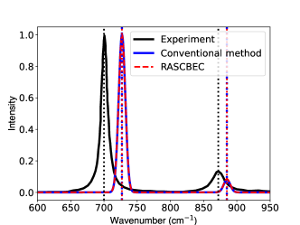
Figure 1: Raman spectra of rutile GeO₂ calculated from the conventional method and RASCBEC (right) compared with experimental Raman (ref. [25]) (left).

Comparison of RASCBEC with the conventional method is shown in Figure 1. The experimental Raman spectrum of rutile GeO₂ measured at $298\,\textrm{K}$ [25] is also included. We can see that the calculated Raman spectra from both calcultional methods exhibit the same two-peak features measured in experiment, but the peak positions are shifted to higher frequencies, as marked by dotted line in Figure 1. The experiment measures two peaks at $700$ cm^-1 and $872$ cm^-1 and from calculation the two peaks are at $727$ cm^-1 and $885$ cm^-1. RASCBEC gives the same result as the conventional method, except that the peak heights differ slightly.

One limit on accuracy is the numerical derivative by electric field. If the applied electric field $\Delta$is too small, the error will be dominated by DFT convergence and round-off errors, but if the field is too large, higher order finite difference errors will become large. A test of the Raman spectra calculated for electric field strengths ranging from $0.025\,\textrm{eV/\AA}$ to $0.2\,\textrm{eV/\AA}$ is shown in Figure 2. It can be seen that relative intensities of the Raman peaks vary with the strength of electric field applied. How the intensity varies with electric field strength is shown in Figure 3 and Figure 4. There is a flat region from $0.05\,\textrm{eV/\AA}$ to $0.125\,\textrm{eV/\AA}$, which means that in this region the computational result is robust. The result shown in Figure 1 used electric field $E=0.1\,\textrm{eV/\AA}$.

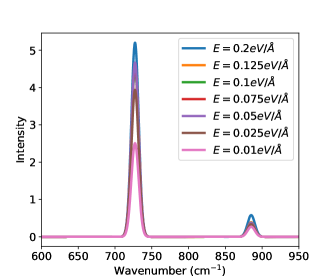
Figure 2: Raman spectra of rutile GeO₂ calculated using different electric fields.

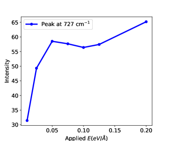
Figure 3: First peak height variation with electric field.

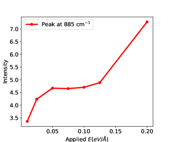
Figure 4: Second peak height variation with electric field.

Timing information for the two methods is provided in Table  1. Note that the estimated time for calculating $\epsilon$ or $Z$ given in the table should be viewed as an upper limit, since all BEC calculations subsequent to the first one take less time. This is because after rotation, only one direction of the electric field needs to be applied instead of 3. The Vienna Ab-initio Simulation Package (VASP)[22, 23] is employed for all first principle calculations. All computations are performed on AMD EPYC 7702.

Table 1: Timing of two methods on crystal (6 atoms)

$N=6$	Number of modes or Z	Average time of getting 1 $\epsilon$ or $Z$	Total time
Dielectric tensor ($\epsilon$)	$6(N-1)=30$	1,700 sec (1 cpu)	51,000 sec
BEC ($Z$)	8	24,886 sec (1 cpu)	200,000 sec

Table 2: Timing of two methods on magnetic molecule (448 atoms)

$N=448$	Number of modes or Z	Average time of getting 1 $\epsilon$ or $Z$	Total time
Dielectric tensor ($\epsilon$)	$6(N-1)=2682$	20,450 sec (32 cpu)	54,846,900 sec
BEC ($Z$)	8	122,860 sec (32 cpu)	982,880 sec

The conventional method calculates the static ion-clamped dielectric matrix using density functional perturbation theory. For a system containing $N$ atoms, there are $3(N-1)$ phonon modes. Two dielectric tensors need to be generated for each phonon mode, displacing the structure in opposite directions, so $2\times 3\times(N-1)=6N-6$ dielectric tensor calculations are needed in total. When $N=6$, this number is 30.

The RASCBEC method differentiating the Born effective charge displaces an electric field in the positive and negative $x$, $y$, $z$ directions as well as the $xy$, $yz$, and $xz$ directions. Since BECs along the $x$, $y$, $z$ directions can be computed in a single calculation, and $-x$, $-y$, $-z$ in another single calculation, 8 BEC are needed in total. This number is independent of $N$.

In summary, if the system size scales to $N$ atoms, then the conventional method will need to generate $6(N-1)$ dielectric tensors. The RASCBEC method needs 8 BEC calculations with electric field applied along different directions. Each BEC calculation with an electric field applied takes about 18 times longer than one without an electric field. Therefore the time ratio of convention method and RASCBEC is $N/8$. When $N$ is greater than 8, RASCBEC has an advantage in computation time.

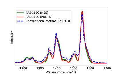
Figure 5: Calculated Raman spectra of Fe_SCO using both the conventional method and RASCBEC

To demonstrate its advantage for large systems, we then apply both the RASCBEC method and conventional method to a large magnetic molecule containing 448 atoms, a recently developed and easily sublimable SCO material, $[Fe(tBu_{2}qsal)_{2}]$ [26]. The computed Raman spectra of this molecule’s low spin state are shown in Figure 5. Red and green lines are the Raman spectra calculated using RASCBEC. To produce the red curve we use PBE+$U$ to calculate BEC, as for the green curve we use hybrid functional. For both ways we applied the electric field $E=0.05\,\textrm{eV/\AA}$. The intensities of these two spectra are normalized with the same normalization factor to compare with a Raman spectra calculated using the conventional method [26]. One can see that in Figure 5 all three curves share the same peak features, in terms of the phonon frequency corresponding to each peak and the relative intensity in general among the peaks. However, one can still identify differences existing at some frequencies. We know that analytically RASCBEC and the conventional method are equivalent. We suspect that this difference comes from the finite differences used to compute derivatives numerically, the derivative of the dielectric tensor for the conventional method and the derivative of the BEC for RASCBEC. When calculating derivatives, all numerical methods make approximations. In solids, these approximations are likely more reliable than in molecules. In molecules, some modes may have substantially large vibrations, and anharmonic effects may become large. However, even when there is strong anharmonicity, we can choose the electric field strength such that response to the electric field is still approximately linear. We see this explicitly in Figures 3 and 4 when the electric field becomes large.

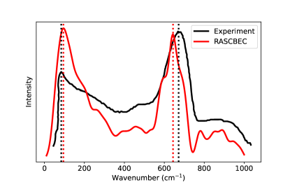
Figure 6: Calculated Raman spectra of amorphous Ta₂O₅ using RASCBEC compared with experiment data [27].

Timing information for two methods is provided in Table  2. All computations are performed on AMD EPYC 7702. The Vienna Ab-initio Simulation Package (VASP) [22, 23] is employed for all first-principle calculations. Regarding the total computation cost, ratio between conventional method and RASCBEC is $54846900/982880=55.8$, and the predicted ratio is $N/8=448/8=56$. We see that RASCBEC is able to save a factor of 56 in computation time for a 448-atom molecule and yet produce Raman spectra with the same accuracy.

Finally we test RASCBEC on large and complex systems: the amorphous materials. Performing thousands of first principle calculations on a large and disordered system can be a daunting task due to the huge computational cost, fortunately we have RASCBEC to handle it. The material we use is Ta₂O₅. An amorphous sample containing 350 atoms is prepared by Molecular Dynamics (MD) simulation using melt-quench method. Classical MD simulation code LAMMPS[28] is used to run the simulation. A classical potential formulated by Trinastic et al. [29] is used to model inter-atomic potential in Ta₂O₅. The calculated and experimental Raman spectra [27] are shown in Figure 6. The black curve is the experiment measurement and the red curve is the Raman spectrum calculated using RASCBEC. Peak positions are denoted with dotted lines. We can clearly see that they both have two main peaks, and the peak positions are very close. In the experiment, the first and second peaks are measured at $84$ cm^-1 and $672$ cm^-1 while from calculation they are at $95$ cm^-1 and $644$ cm^-1. The computation time of one BEC on AMD EPYC 7702 is about $65,540$ secs on $256$ cpu, so the total cost is $524,320$ secs. To have a taste of the conventional method on amorphous materials, we also tried one dielectric tensor calculation and it takes $52,170$ secs on $256$ cpu. $2094$ such calculations are needed so the total required computation time is about $109,243,980$ secs. This is much too expensive to carry through to the finish.

IV Conclusion

In conclusion, in this paper we have introduced a newly developed method of calculation of Raman spectra using an electric field derivative of the Born effective charge to replace the sum over phonon modes of polarizability derivatives along mode eigenvectors used in the conventional method. We call the new method the RASCBEC. Since for large systems there is a large number of terms in the polarizability sum, this allows us to expedite first-principles Raman calculation and probe large systems in an economical way. This method saves computation time for large systems by a factor of $N/8$, where $N$ is the number of atoms in the simulation box. Tests of the RASCBEC method on an atomic crystal, a large magnetic molecule, and a large amorphous system verify its ability to reproduce the results of the conventional method and its significant reduction in computational cost. Applying this method to even larger and more complex systems to calculate Raman activity is possible, and we will explore more directions in the future.