Robust Mode Connectivity-Oriented Adversarial Defense: Enhancing Neural Network Robustness Against Diversified $\ell_{p}$ Attacks

Abstract

Adversarial robustness is a key concept in measuring the ability of neural networks to defend against adversarial attacks during the inference phase. Recent studies have shown that despite the success of improving adversarial robustness against a single type of attack using robust training techniques, models are still vulnerable to diversified $\ell_{p}$ attacks. To achieve diversified $\ell_{p}$ robustness, we propose a novel robust mode connectivity (RMC)-oriented adversarial defense that contains two population-based learning phases. The first phase, RMC, is able to search the model parameter space between two pre-trained models and find a path containing points with high robustness against diversified $\ell_{p}$ attacks. In light of the effectiveness of RMC, we develop a second phase, RMC-based optimization, with RMC serving as the basic unit for further enhancement of neural network diversified $\ell_{p}$ robustness. To increase computational efficiency, we incorporate learning with a self-robust mode connectivity (SRMC) module that enables the fast proliferation of the population used for endpoints of RMC. Furthermore, we draw parallels between SRMC and the human immune system. Experimental results on various datasets and model architectures demonstrate that the proposed defense methods can achieve high diversified $\ell_{p}$ robustness against $\ell_{\infty}$, $\ell_{2}$, $\ell_{1}$, and hybrid attacks. Codes are available at https://github.com/wangren09/MCGR.

1 Introduction

The last decade has seen a rapid development of deep learning techniques, which are now widely applied in areas like medical imaging [1], defect detection [2], and power systems [3] that require high security. As the key component of deep learning, neural networks (NNs) learn the desired mappings from a set of data. Although NNs may accurately identify the underlying relationship in the provided data, their decisions are sensitive to even little changes in the inputs, known as adversarial perturbations [4, 5]. The perturbed data are called adversarial examples, which show no difference to human eyes compared with their clean counterparts. Such a vulnerability raises questions about how users can trust these models in high-security applications [6, 7].

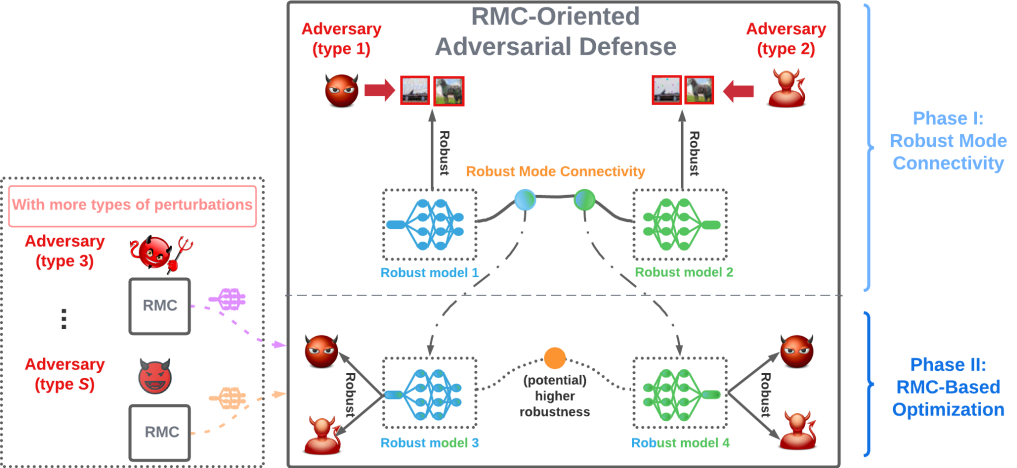
Figure 1: Overview of the Robust Mode Connectivity (RMC)-Oriented Adversarial Defense. The upper level of the panel shows Phase I of the framework, illustrating that a robust path (robust to adversary types 1 and 2) in the parameter space can be found by connecting one model robust to adversary type 1 and the second model robust to adversary type 2. Selecting optimal points from the path and implementing the RMC process again can further improve robustness, as illustrated in the lower level of the panel. Phase II suggests that more adversary types can be considered by using RMC as the basic unit.

Extensive research has lately been conducted to solve the vulnerability issue of NNs. Among all works, adversarial training and its variants have demonstrated cutting-edge performance [6, 8, 9, 10]. The main idea of adversarial training is to update NNs with continuously generated adversarial examples from the clean training data. Therefore, NNs learn the adversarial distributions and are able to maintain a certain level of robustness in the inference phase. However, most of the existing works consider a single type of $\ell_{p}$ norm perturbation during adversarial training, resulting in the rapid decline of robustness when facing inputs with perturbations that are different from the one used in training [11]. Although a few works have attempted to address the issues by training NNs with multiple $\ell_{p}$ norm perturbations [12, 13, 11, 14, 15, 16], they have not yet completely resolved the issue of lack of diversified $\ell_{p}$ robustness, most likely because traditional neural network learning mechanisms rely on optimization on a single set of parameters, and involving sampling and evaluating individual points in the search space. When dealing with multiple robustness objectives, limited search capabilities may trap conventional learning mechanisms in local minima or saddle points where the gradient is close to zero, but the loss function is not yet optimized. This can prevent the network from achieving the global minimum of our robustness objective. In contrast to conventional neural network learning methods, population-based optimization can explore a broader range of solutions by maintaining a diverse population of candidate solutions, which can lead to better overall results [17, 18, 19]. Additionally, population-based optimization can be used to optimize complex problems, such as the problem of achieving diversified $\ell_{p}$ robustness, that traditional methods cannot handle. Recent works find the mode connectivity property that a low-loss high-accuracy path connected by two well-trained models exists in the parameter space [20, 21]. The method of finding the path can be viewed as an accelerated population-based optimization strategy, which finds a large number of candidates on the path. However, simply adopting the method will fail in the adversarial setting.

The major goal of this work is to achieve models’ diversified $\ell_{p}$ robustness against perturbations generated by attacks constrained on $\ell_{p}$ norms (In this work we consider $p=1,2,\infty$). Spurred by the mode connectivity property and our hypothesis that the diversified $\ell_{p}$ robustness of conventional training methods is limited by insufficient space search, we propose a robust mode connectivity-oriented adversarial defense that utilizes two-phase population-based optimization. In Phase I of the defense, we develop a robust mode connectivity (RMC) method by implementing the idea of mode connectivity and leveraging a multi steepest descent (MSD) algorithm [14] to find a path of NNs with high robustness against different perturbations, as shown in Figure 1 panel of RMC. In Phase II, RMC serves as a basic unit of a bigger regime - an RMC-based optimization, which is also illustrated in Figure 1. RMC-based optimization selects models with high diversified $\ell_{p}$ robustness from the population generated by each RMC module. To improve the efficiency of the RMC-based optimization, we further incorporate a self-robust mode connectivity (SRMC) module to RMC-based optimization. We point out that there exists a strong connection between RMC-based optimization and the human immune system.

Contributions. We propose a robust mode connectivity-oriented adversarial defense that includes the following main contributions:

• We have developed a robust mode connectivity (RMC) method that can find a path connecting two adversarially trained models with high robustness against diversified $\ell_{p}$ norm perturbations. (Experimental results are given in Figs 4, 6, 7, 8, 13, 14)

• Building on the multi-stage RMC, we have developed an RMC-based optimization method that generates a larger population of candidates. This method further boosts the diversified $\ell_{p}$ robustness of neural networks by selecting the optimal models. (Experimental results can be viewed in Figs 9, 10, 11)

• We propose a self-robust mode connectivity (SRMC) module as an efficient strategy to enhance RMC-based optimization. (Experimental results are shown in Figs 12, 15, 16)

• We conduct a comprehensive study of the RMC and RMC-based optimization, showing that the proposed methods can achieve higher diversified $\ell_{p}$ robustness than the baselines. (see Table I)

The rest of this article is organized as follows. Section 2 introduces related works on defenses against diversified $\ell_{p}$ norm perturbations and population-based neural network learning. In Section 3, we provide the definition of diversified $\ell_{p}$ robustness, and give introductions to adversarial attack, adversarial training, and mode connectivity. Sections 4 and 5 introduce the two phases of the proposed mode connectivity-oriented adversarial defense. The RMC method is presented in Section 4. The RMC-based optimization and SRMC are proposed in Section 5. Section 6 shows the experimental results. Section 7 concludes the article.

2 Related Work

2.1 Defenses on Diversified $\ell_{p}$ Norm Perturbations

Among all the works, [12] is the only work that provides a provable defense, and [13] considers withholding specific inputs to improve model resistance to stronger attacks. [11] designs the inner loss by selecting the type of perturbation that provides the maximum loss or averaging the loss on all types of perturbations. According to the report from a recent work [15], [14] is the existing SOTA method for achieving diversified $\ell_{p}$ robustness. [14] includes the various perturbation models within each step of the projected steepest descent in order to produce an adversary with complete knowledge of the perturbation region. Nevertheless, despite their efforts, all the aforementioned works still depend on optimizing a single set of parameters, and the challenge of addressing the deficiency in diversified $\ell_{p}$ robustness remains unresolved. This work solves the challenge from a population-based optimization perspective.

2.2 Population-Based Neural Network Learning

Optimizing a population of neural networks instead of a single network can prevent getting stuck at local minimums and lead to improved results. In one approach, [22] trained multiple instances of a model in parallel and selected the best performing instances to breed new ones. [23] proposed an evolutionary stochastic gradient descent method that improved upon existing population-based methods. However, such methods typically have low learning speed and neglect adversarial robustness. Inspired by the human immune system, researchers have mimicked the key principles of the immune system in the inference phase to increase the robustness and not affect the learning speed in the training phase [24]. Mode connectivity can be treated as a faster population-based learning with two ancestor models that enhances the learning efficiency in the training phase [21]. Researchers also analyze the mode connectivity when networks are tampered with backdoor or error-injection attacks or under the attack of a single type of perturbation [25]. To defend against multiple adversarial strategies, it would be interesting to explore incorporating different adversarial strategies into the learning of mode connectivity and generalize it for mode connectivity-based optimization.

3 Preliminaries

3.1 Adversarial Attack with Different Input Perturbation Generators

Recent studies show that conventional learning methods suffer from perturbed datasets ($\mathcal{D}_{1},\mathcal{D}_{2},\cdots,\mathcal{D}_{S}$) generated by

$$\displaystyle\arg\max{\mathcal{L}(\boldsymbol{\theta};\bf x^{\prime},y)},~{}~{}s.t.~{}~{}\text{Dist}_{i}(\bf x^{\prime},\bf x)\leq\delta_{i},$$ (1)

for $\forall\bf x\in\mathcal{D}_{0}$, where $\mathcal{D}_{0}$ denotes the benign dataset and $\delta_{i}$s are sufficient small values. This is usually referred to as an adversarial attack [6]. In this paper, we restrict distance measures $\text{Dist}_{i}$s to be $\ell_{p},p=1,2,\infty$ norms. A practical way to solve (1) is to apply gradient descent and projection $P_{\delta_{i}}$ that maps the perturbation $\boldsymbol{\epsilon}_{i}=\bf x^{\prime}-\bf x$ to a feasible set, which is usually referred to as PGD attack. We will use $\ell_{p}$-PGD to denote the PGD attack with the $\ell_{p}$ norm.

3.2 Adversarial Training (AT)

The min-max optimization-based adversarial training (AT) is known as one of the most powerful defense methods to obtain a robust model against adversarial attacks [6]. We summarize AT below:

$$\begin{array}[]{ll}\displaystyle\min_{\boldsymbol{\theta}}\mathbb{E}_{(\mathbf{x},y)\in\mathcal{D}_{0}}[\displaystyle\max_{\text{Dist}_{i}(\bf x^{\prime},\bf x)\leq\delta_{i}}\mathcal{L}(\boldsymbol{\theta};\mathbf{x}^{\prime},y)],\end{array}$$ (3)

Although AT can achieve relatively high robustness on $\mathcal{D}_{i}$, it does not generalize to other $\mathcal{D}_{j},j\not=i$. Moreover, training on all $\mathcal{D}_{i},i\in[S]$ is not scalable and will not provide robustness to all types of perturbations [11]. We will use $\ell_{p}$-AT to denote the AT with the $\ell_{p}$ norm.

3.3 Definition of Diversified $\ell_{p}$ Robustness

We hope that models can be robust to every $\ell_{p}$ adversarial type in the adversarial set of concerns, and we need to give a metric to measure such robustness. Diversified $\ell_{p}$ Robustness (DLR) is defined as its capacity to sustain the worst type of perturbation confined by a specific level of attack power:

Definition 1

For a loss function $\mathcal{L}$ and a benign dataset $\mathcal{D}_{0}$, the Diversified $\ell_{p}$ Robustness of a set of neural network parameters $\boldsymbol{\theta}$ is

$$\frac{\min_{i\in[S]}\sum_{(\bf x^{\prime},y)\in\mathcal{D}_{i}}\boldsymbol{1}_{f(\bf x^{\prime},\boldsymbol{\theta})=y}}{|\mathcal{D}_{i}|},$$ (4)

where $\mathcal{D}_{i}$ represents the data generated by (1) with $\textup{Dist}_{i}$ as one of $\ell_{p},p=1,2,\infty$ norms. We remark that there are other ways to define DLR. For example, the definition can be based on the worst-case sample-wise instead of worst-case data set-wise. Despite the difference, they essentially measure the same quantity, i.e., how well the model performs under various types of $\ell_{p}$ perturbations.

3.4 Nonlinear Mode Connectivity

Figure 2: The path with near-constant loss found by mode connectivity in the parameter space. The endpoints are two pre-trained models.

Mode connectivity is a neural network’s property that local minimums found by gradient descent methods are connected by simple paths belonging to the parameter space [20, 21]. Everywhere on the paths achieves a similar cost as the endpoints. The endpoints are two sets of neural network parameters $\boldsymbol{\theta}_{1},\boldsymbol{\theta}_{2}\in\mathbb{R}^{d}$ with the same structure and trained by minimizing the given loss $\mathcal{L}$. The smooth parameter curve is represented using $\phi(t;\boldsymbol{\theta})\in\mathbb{R}^{d},t\in[0,1]$, such that $\phi(0;\boldsymbol{\theta})=\boldsymbol{\theta}_{1},\phi(1;\boldsymbol{\theta})=\boldsymbol{\theta}_{2}$. To find a desired low-loss path between $\boldsymbol{\theta}_{1}$ and $\boldsymbol{\theta}_{2}$, it is proposed to find parameters that minimize the following expectation over a uniform distribution on the curve.

$$\min_{\boldsymbol{\theta}}\mathbb{E}_{t\sim q(t;\boldsymbol{\theta})}\displaystyle\mathbb{E}_{(\bf x,y)\sim\mathcal{D}_{0}}\mathcal{L}(\phi(t;\boldsymbol{\theta});(\bf x,y)),$$ (5)

where $q(t;\boldsymbol{\theta})$ represents the distribution for sampling the parameters on the path. Note that (5) is generally intractable. A computationally tractable surrogate is proposed as follows

$$\min_{\boldsymbol{\theta}}\mathbb{E}_{t\sim U(0,1)}\displaystyle\mathbb{E}_{(\bf x,y)\sim\mathcal{D}_{0}}\mathcal{L}(\phi(t;\boldsymbol{\theta});(\bf x,y)),$$ (6)

where $U(0,1)$ denotes the uniform distribution on $[0,1]$. Two common choices of $\phi(t;\boldsymbol{\theta})$ in nonlinear mode connectivity are the Bezier curve [26] and Polygonal chain [27]. As an example, a quadratic Bezier curve is defined as $\phi(t;\boldsymbol{\theta})=(1-t)^{2}\boldsymbol{\theta}_{1}+2t(1-t)\boldsymbol{\theta}+t^{2}\boldsymbol{\theta}_{2}$. Training neural networks on these curves provides many similar-performing models on low-loss paths. As shown in Fig. 2, a quadratic Bezier curve obtained from (6) connects the upper two models along a path of near-constant loss.

4 Phase I: Robust Path Search Via Robust Mode Connectivity

4.1 A Pilot Exploration

Mode connectivity and adversarial training seem to be two excellent ideas for achieving high DLR that has been defined in Definition 1. If we set $\phi(0;\boldsymbol{\theta})$ and $\phi(1;\boldsymbol{\theta})$ to be two adversarially-trained neural networks under different types of perturbations, applying (6) may result in a path with points having high robustness for all these perturbations. Thus we ask:

(Q1) Can simply combining adversarial training with mode connectivity provide high DLR?

Here we aim to see if implementing vanilla mode connectivity can bring us high DLR. We combine two PreResNet110 models [28], one trained with $\ell_{\infty}$-AT ($\delta=8/255$, 150 epochs) and the other trained with $\ell_{2}$-AT ($\delta=1$, 150 epochs), to find the desired path using the vanilla mode connectivity (6). $\phi(0;\boldsymbol{\theta})$ and $\phi(1;\boldsymbol{\theta})$ are models trained by $\ell_{\infty}$-AT and $\ell_{2}$-AT, respectively. The mode connectivity curve is obtained with additional 50 epochs of training. The results are shown in Figure 3. The left (right) endpoint represents the model trained with $\ell_{\infty}$-AT ($\ell_{2}$-AT). One can see that the path has high loss and low robust accuracies on both types of attacks, indicating that vanilla mode connectivity fails to find the path that enjoys high DLR.

Figure 3: The vanilla mode connectivity (6) with models trained by $\ell_{\infty}$-AT and $\ell_{2}$-AT as two endpoints fails to find the path with high DLR. $\phi(0;\boldsymbol{\theta})$ and $\phi(1;\boldsymbol{\theta})$ are $\ell_{\infty}$-AT ($\delta=8/255$, 150 epochs) and $\ell_{2}$-AT ($\delta=1$, 150 epochs).

4.2 Embedding Adversarial Robustness to Mode Connectivity

Although the vanilla mode connectivity aims to provide insight into the loss landscape geometry, it searches space following the original data distribution. Therefore it cannot provide high DLR by simply using two adversarially-trained models as two endpoints. Instead, we ask:

(Q2) Can we develop a new method to embed adversarial robustness to mode connectivity by searching the adversarial input space?

To answer (Q2), we connect mode connectivity (6) with adversarial training under diversified $\ell_{p}$ adversarial perturbations. In other words, we modify the objective (6) to adjust to our high DLR purpose. An adversarial generator is added as an inner maximization loop. We adopt different types of perturbations in the generator. This is because a single type of perturbation may result in robustness bias. Formally, we obtain a model path $\phi(t;\boldsymbol{\theta}),t\in[0,1]$ parameterized by $\boldsymbol{\theta}$.

$$\min_{\boldsymbol{\theta}}\mathbb{E}_{t\sim U(0,1)}\displaystyle\mathbb{E}_{(\bf x,y)\sim\mathcal{D}_{0}}\sum_{i\in I}\max_{\text{Dist}_{i}(\bf x^{\prime},\bf x)\leq\delta_{i}}\mathcal{L}(\phi(t;\boldsymbol{\theta});(\bf x^{\prime},y)),$$ (7)

where $\phi(0;\boldsymbol{\theta})$ and $\phi(1;\boldsymbol{\theta})$ are two models trained by (3), probably under different types of perturbations. Throughout this paper, we fix the curve as a quadratic Bezier curve. Thus a model at the point $t$ can be represented by $\phi(t;\boldsymbol{\theta})=(1-t)^{2}\boldsymbol{\theta}_{1}+2t(1-t)\boldsymbol{\theta}+t^{2}\boldsymbol{\theta}_{2}$. Similar to the nonlinear mode connectivity, (7) is a computationally tractable relaxation by directly sampling $t$ from the uniform distribution $U(0,1)$ during the optimization. Data points $(\bf x^{\prime},y)$ are generated from a union of adversarial strategies $i\in I$, where $I$ is a subset of $\{1,2,3,\cdots,S\}$. For example, data can be generated by using $\ell_{2}$ or $\ell_{\infty}$ norm distance measure, which is commonly used in adversarial attacks and adversarial training. Formulation in (7) guarantees that the path we found always adjusts to those concerned adversarial perturbations.

We call (7) the Robust Mode Connectivity (RMC), which serves as the first defense phase for robust path search. We remark that RMC itself is a defense method as we can select the model with the highest DLR in the path. One can see that a group of models (all points in the path) are generated from two initial models. Therefore RMC is a population-based optimization. The next step is to find out how to solve the RMC (7).

Algorithm 1 Robust Mode Connectivity

0  $\phi(0;\boldsymbol{\theta})$, $\phi(1;\boldsymbol{\theta})$ - two selected models with the same structure (potentially trained with different strategies, e.g., AT under different perturbation types); initial model $\boldsymbol{\theta}^{0}$; the perturbation types $i\in I$ and the corresponding projections $P_{\delta_{i}}$; training set $\mathcal{D}_{0}$; inner loop iteration number $J$; batch size $B$; initial perturbation $\epsilon^{(0)}=\mathbf{0}$.

1  $\boldsymbol{\theta}=\boldsymbol{\theta}^{0}$.

2  For each data batch $\mathcal{D}_{b}\in\mathcal{D}_{0}$ in each epoch $e\in E$, do

3  Uniformly select $t\sim U(0,1)$.

4  For $\forall\bf x\in\mathcal{D}_{b}$, do

5  for $j=1,\cdots,J$ do

6     for $i\in I$ do

7        $\boldsymbol{\epsilon}_{i}^{(j)}\leftarrow P_{\delta_{i}}\big{(}\boldsymbol{\epsilon}^{(j-1)}-{\nabla_{\boldsymbol{\epsilon}}\mathcal{L}(\phi(t;\boldsymbol{\theta});\bf x+\boldsymbol{\epsilon}^{(j-1)},y)}\big{)}$.

8     end for

9     $\boldsymbol{\epsilon}^{(j)}\leftarrow\arg\max_{\boldsymbol{\epsilon}_{i}^{(j)},i\in I}{\mathcal{L}(\phi(t;\boldsymbol{\theta});\bf x+\boldsymbol{\epsilon}_{i}^{(j)},y)}$.

10  end for

11  end For

12  $\boldsymbol{\theta}\leftarrow\boldsymbol{\theta}-\nabla_{\boldsymbol{\theta}}\sum_{\bf x\in\mathcal{D}_{b}}\mathcal{L}(\phi(t;\boldsymbol{\theta});\bf x+\boldsymbol{\epsilon}^{(j-1)},y)$

13  end For

14  Return:  $\boldsymbol{\theta}$, $\phi(t;\boldsymbol{\theta}),\forall t\in[0,1]$

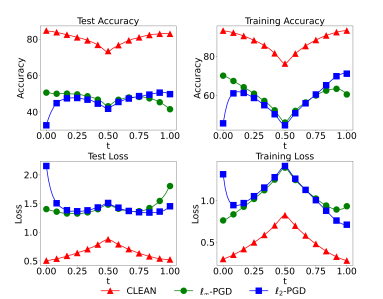
(a) Epoch=50

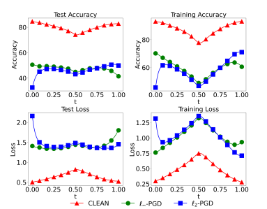
(b) Epoch=100

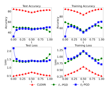
(c) Epoch=150

Figure 4: The RMC (7) with models trained by $\ell_{\infty}$-AT and $\ell_{2}$-AT as two endpoints can find the path with high DLR. MSD [14] with perturbations generated by $\ell_{2}$ and $\ell_{\infty}$ norm distance measures is leveraged as the inner solver. Solving (7) uses 50/100/150 epochs in panel (a)/(b)/(c).

4.3 Solving Robust Mode connectivity Via Multi Steepest Descent

Solving (7) is difficult as it contains multi-type perturbations. The simplest ways are using ‘MAX’ or ‘AVG’ strategy proposed in [11], where the inner loss is obtained by selecting the type of perturbation that provides the maximum loss or averaging the loss on all types of perturbations. However, both strategies consider perturbations independently. We leverage a Multi Steepest Descent (MSD) approach that includes the various perturbation models within each step of the projected steepest descent in order to produce a PGD adversary with complete knowledge of the perturbation region [14]. The key idea is to simultaneously maximize the worst-case loss overall perturbation models at each step. Algorithm 1 shows the details, where all the perturbation types are considered in each iteration. Next we test the effectiveness of the proposed RMC algorithm.

We again use models trained with $\ell_{\infty}$-AT ($\delta=8/255$, 150 epochs) and $\ell_{2}$-AT ($\delta=1$, 150 epochs) as two endpoints $\phi(0;\boldsymbol{\theta})$ and $\phi(1;\boldsymbol{\theta})$. The RMC (7) with MSD as the inner solver is applied to obtain the path. Figure 4 shows the results of training an additional 50/100/150 epochs with $D_{i}$s generated by $\ell_{2}$ and $\ell_{\infty}$ norm distance measures. One can find that unlike Figure 3, the paths contain points with high accuracy and high robustness against both $\ell_{\infty}$-PGD and $\ell_{2}$-PGD attacks. Although the left endpoint has low $\ell_{2}$ robustness and the right endpoint has relatively low $\ell_{\infty}$ robustness, they can achieve high DLR in the connection, where the highest DLR is $48.19\%$ in panel (a). One can also notice that when the epoch number for solving (7) increases, the path becomes smoother. Another finding is that the optimal points in panels (a), (b), and (c) have similar DLR. The experiments indicate that RMC can find a path with high DLR. If the goal is to select an optimal model from the path, it is enough to only conduct the training with a small number of epochs.

5 Phase II: Robust Model Selection Via Robust Mode Connectivity-Based Optimization

Algorithm 2 Robust Mode Connectivity-Based Optimization ($\ell_{1},\ell_{2},\ell_{\infty}$ perturbations)

1  Train three models for $T$ epochs using $\ell_{1},\ell_{2},\ell_{\infty}$ perturbations, respectively. (Training can be accelerated using the SRMC module proposed in Section 5.2)

2  Apply Algorithm 1 with $\ell_{2},\ell_{1}$-AT trained models ($I$ includes $\ell_{2},\ell_{1}$) and $\ell_{\infty},\ell_{1}$-AT trained models ($I$ includes $\ell_{\infty},\ell_{1}$) as $\phi(0;\boldsymbol{\theta})$, $\phi(1;\boldsymbol{\theta})$, and return model trajectories $\phi_{\boldsymbol{\theta}-\ell_{\infty}}(t),\phi_{\boldsymbol{\theta}-\ell_{2}}(t),\forall t\in[0,1]$. (pairs of perturbations can be selected in different ways)

3  Randomly pick points $t_{-\ell_{\infty}}$, $t_{-\ell_{2}}$ from optimal regions for each model trajectory.

4  Train models for $T$ epochs using $\ell_{\infty},\ell_{2}$ perturbations starting from $\phi_{\boldsymbol{\theta}-\ell_{\infty}}(t_{-\ell_{\infty}}),\phi_{\boldsymbol{\theta}-\ell_{2}}(t_{-\ell_{2}})$, respectively.

5  Apply Algorithm 1 with the two models as $\phi(0;\boldsymbol{\theta})$, $\phi(1;\boldsymbol{\theta})$ with $I$ including $\ell_{1},\ell_{2},\ell_{\infty}$ perturbations.

6  Find the optimal point $t_{\text{opt}}$ from the model trajectory.

7  Return:  $\phi_{\boldsymbol{\theta}}(t_{\text{opt}})$

5.1 From RMC to RMC-Based Optimization

Suppose we have neural networks that share the same structure but are trained with different settings, e.g., different types of perturbations, perturbation magnitudes, learning rates, batch size, etc. In that case, we can use RMC to search for candidates potentially leading us to better solutions or even global optimums. The intuition behind the claim is that low-loss & high-DLR paths connect all the minimums, and thus it becomes easier for search algorithms to jump out of the sub-local minimums. We have seen the exciting property of the proposed RMC, which indicates that a larger population of NNs can result in higher DLR. Notice that RMC can serve as a component in a larger population-based optimization to select robust models with higher DLR. A natural question to ask is:

(Q3) Can we develop a general population-based optimization method built on RMC modules to further improve the DLR of a single RMC?

The RMC-based optimization we developed below includes an evolving process of RMC units for multiple generations. As a starting point, we generate an initial population by training neural networks with data points augmented using different $\text{Dist}_{i}$ in (3). We use gradient descent to train these networks but pause the training when specific stop criteria have been met, e.g., the number of epochs or accuracy achieving the preset threshold. The initial population then varies, and the system selects candidates with the best performances. The two operations in our approach are unified through the RMC that connects two adversarially-trained neural network models on their loss landscape using a high-accuracy & high-DLR path characterized by a simple curve. Candidates for the next generation are selected among the high DLR points on the curve. The process can be repeated and an optimal solution that enjoys the highest DLR is selected among the final candidates.

Algorithm 2 shows the pipeline using an example of three types of perturbations. We first train three models with $\ell_{\infty}$-AT, $\ell_{2}$-AT, and $\ell_{1}$-AT for $T$ epochs. We then connect the $\ell_{2}$-AT model with the $\ell_{1}$-PGD model and connect the $\ell_{\infty}$-AT model with the $\ell_{1}$-AT model using the RMC for some additional epochs. The two model trajectories are denoted by $\phi_{\boldsymbol{\theta}-\ell_{\infty}}(t)$ and $\phi_{\boldsymbol{\theta}-\ell_{2}}(t),\forall t\in[0,1]$. Notice that the curves will not be perfectly flat. But there exist some regions containing points with high DLR. We will randomly pick a model from a small optimal region in each curve. In practice, we will find the point with the highest DLR and randomly pick a point around the optimal point. The rationale behind this is to increase diversity during the training. After obtaining the models $\phi_{\boldsymbol{\theta}-\ell_{\infty}}(t_{-\ell_{\infty}})$ and $\phi_{\boldsymbol{\theta}-\ell_{2}}(t_{-\ell_{2}})$ from both trajectories, the two new endpoints are obtained by training each model $T$ epochs using the $\ell_{p}$-AT that is different from the types used in the previous RMC. In this specific case, we use $\ell_{\infty}$-AT and $\ell_{2}$-AT. Finally, we connect the two new endpoints with RMC for some additional epochs and find the new optimum $\phi_{\boldsymbol{\theta}}(t_{\text{opt}})$ at $t_{\text{opt}}$. In the case of two types of perturbations, one can start to train two models from a single optimal point or train one model from each of the two optimal points. We refer readers to Section 6.3 for more details. In a more general scenario where there are $S$ types of perturbations, the process is the same, except that it contains more RMC units, as illustrated in Figure 1. We learn optimal points from pairs of models trained by AT under different perturbations and finally find an optimal point with the highest DLR.

5.2 Improving Learning Efficiency of the RMC-Based Optimization With a Self-Robust Mode Connectivity Module

One drawback of the previous scheme is that it needs to initially pre-train multiple neural networks ($\geq S$ models), which could be slow when the computational resources are limited. We ask:

(Q4) How can we accelerate the learning process of the RMC-based optimization?

Here we propose to replace RMC with a self-robust mode connectivity (SRMC) module in the learning process. SRMC can accelerate the endpoints training in the path search process and thus speed up RMC-based optimization. We start with one set of neural network parameters $\phi(0;\boldsymbol{\theta})=\boldsymbol{\theta}_{1}$ that is trained by (3) with a fixed $\text{Dist}_{i}$. After the model achieves high robustness on $\mathcal{D}_{i}$, we retrain the model for a few epochs using (3) with $\text{Dist}_{j}$. The new model we obtained will be placed at the endpoint $\phi(1;\boldsymbol{\theta})=\boldsymbol{\theta}_{2}$. Now the low-loss high-robustness path can be found by optimizing (7). By leveraging the SRMC module, our proposed framework yields both high DLR and learning efficiency.

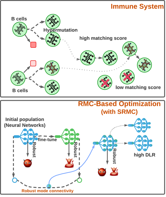
Figure 5: RMC-based optimization with SRMC modules can be viewed as a computational parallel of the human immune system. After encountering a pathogen, the immune system initiates the proliferation of B cells through somatic hypermutation, whereby a larger population of B cells is generated. Then B cells with higher matching scores to the pathogen are chosen to create new B cells. Through a process similar to the immune process, RMC-based optimization with SRMC modules generates models from a single model and finds the optimal path by connecting a pair of models. Subsequently, models with higher DLR are selected as candidates.

Comparison with the human immune system. RMC-based optimization with SRMC can also be viewed as a computational parallel of the human immune system [29], as illustrated in Fig. 5. When the immune system is exposed to a pathogen, B cells undergo somatic hypermutation to proliferate and form a larger population. B cells with higher matching scores to the pathogen are then chosen to produce new B cells, which is analogous to the RMC-based optimization process with SRMC modules. In this optimization process, hypermutation represents the creation of models from a single model and the identification of the optimal path through connecting a pair of models. The selection of candidates with higher DLR follows a similar pattern to the immune system’s selection of effective defenses against diverse pathogens. Consequently, like the immune system, RMC-based optimization can produce models that are resistant to a range of attacks.

6 Experimental Results

Figures 3, 4 show that using the proposed RMC can find a path with points in it enjoying high robustness on diversified $\ell_{p}$ perturbations. In this section, we conduct more comprehensive experiments on two phases of the Robust Mode Connectivity-Oriented Adversarial Defense.

6.1 Settings

We validate our proposed methods on CIFAR-10 and CIFAR-100 datasets [30] using PreResNet110 and WideResNet-28-10 architectures. The perturbation types $\textup{Dist}_{i}$s considered in this work are $\ell_{\infty}$, $\ell_{2}$, and $\ell_{1}$ norms with perturbation constrained by $\delta=8/255,1$, and $12$, respectively. We use AT to obtain endpoints’ models. We compare our methods with the standard $\ell_{\infty}$-AT baseline and the state-of-the-art method MSD [14]. The evaluation methods include basic PGD adversarial attacks under $\ell_{\infty}$, $\ell_{2}$, $\ell_{1}$ norm perturbations and MSD attack. The evaluation metrics are (1) standard accuracy on clean test data; (2) robust accuracies under $\ell_{\infty}$, $\ell_{2}$, $\ell_{1}$-PGD adversarial attacks and MSD; (3) accuracy on worst-case sample-wise (Union) using all three basic PGD adversarial attacks; and (4) DLR on $\ell_{\infty}$, $\ell_{2}$, $\ell_{1}$-PGD adversarial attacks for three types of perturbations and DLR on $\ell_{\infty}$, $\ell_{2}$ for two types of perturbations. All the following experiments are conducted on two NVIDIA RTX A100 GPUs.

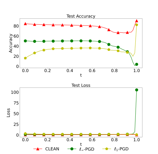
Figure 6: Curves obtained from two models trained by $\ell_{1}$-AT and $\ell_{\infty}$-AT contain points with higher DLR on $\ell_{1}$ and $\ell_{\infty}$-PGD attacks. The paths are obtained by training 50 epochs. The two endpoints are trained for 150 epochs.

Figure 7: Curves obtained from two models trained by $\ell_{1}$-AT and $\ell_{2}$-AT contain points with higher DLR on $\ell_{1}$ and $\ell_{2}$-PGD attacks. The paths are obtained by training 50 epochs. The two endpoints are trained for 150 epochs. $\ell_{2}$-AT trained model can also provide a relatively high level of robustness against the $\ell_{1}$-PGD attack.

6.2 A More Comprehensive Study of the Robust Mode Connectivity

In this subsection, we aim to study the effectiveness of the proposed method (7) on different models. We will consider models trained under various settings. By default, we train endpoints’ models 50/150 epochs and the paths are obtained by training an additional 50 epochs. Experiments on pairwise combinations of $\ell_{\infty}$, $\ell_{2}$, $\ell_{1}$-AT trained models are conducted. We also show results on CIFAR-100 and WideResNet-28-10 CNN architecture.

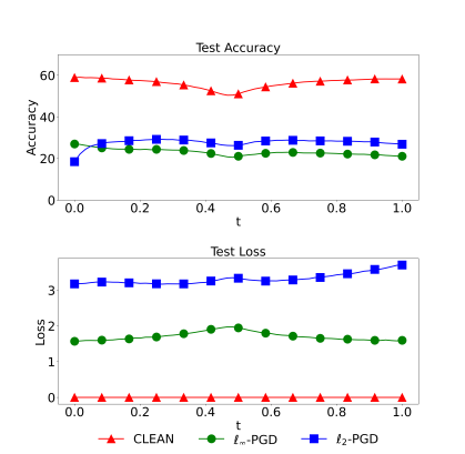
(a) CIFAR100

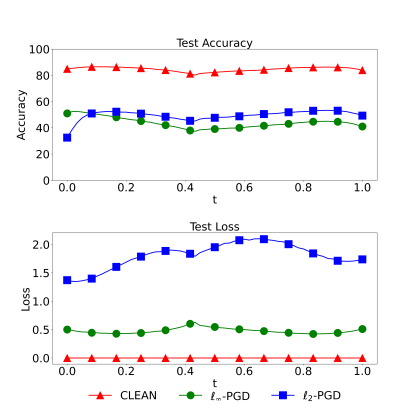
(b) WideResNet-28-10

Figure 8: RMC can find paths containing points with high DLR on different datasets and model architectures. The left (right) figure shows that RMC performs well on CIFAR-100 dataset (WideResNet-28-10 architecture). The paths are obtained by training 50 epochs with two endpoints trained with $\ell_{\infty}$ and $\ell_{2}$-AT.

$\ell_{\infty}$-AT trained model with $\ell_{1}$-AT trained model. We consider an additional $\ell_{1}$-AT trained model and combine it with the $\ell_{\infty}$-AT trained model. The results are shown in Fig. 6. Two endpoints are trained for 150 epochs and the path is obtained by additional 50 epochs. It can be seen that the right endpoint, i.e., the $\ell_{1}$-AT trained model, has a high resilience to $\ell_{1}$ perturbations but suffers from $\ell_{\infty}$ perturbations. The left endpoint, i.e., the $\ell_{\infty}$-AT trained model, has a high resilience to $\ell_{\infty}$ perturbations and also can defend against a certain level of $\ell_{1}$ perturbations. By applying the RMC, we obtain a path with enhanced DLR against both two attacks.

$\ell_{2}$-AT trained model with $\ell_{1}$-AT trained model. We then consider the combination between the $\ell_{1}$-AT trained model and the $\ell_{2}$-AT trained model. The results are shown in Fig. 7. One can see that the model of $\phi(1;\boldsymbol{\theta})$, i.e., the $\ell_{1}$-AT trained model has high robustness against the $\ell_{1}$-PGD attack, but has almost no resilience against the $\ell_{2}$-PGD attack. The model of $\phi(0;\boldsymbol{\theta})$, i.e., the $\ell_{2}$-AT trained model can achieve a slightly higher (almost the same) robustness on $\ell_{2}$-PGD perturbations than $\ell_{2}$-PGD perturbations. From the DLR perspective, $\phi(0;\boldsymbol{\theta})$ is a more robust model. By connecting the $\phi(0;\boldsymbol{\theta})$ with $\phi(1;\boldsymbol{\theta})$, a path with a higher robustness region can be achieved. One can also see that the $\ell_{2}$-AT trained model can also provide a relatively high level of robustness against the $\ell_{1}$-PGD attack.

RMC on CIFAR-100 and WideResNet-28-10. Here we evaluate the effectiveness of RMC on CIFAR-100 and WideResNet-28-10 model architecture. We consider two types of perturbations that are generated from $\ell_{\infty}$ and $\ell_{2}$-PGD attacks. Endpoints are trained for 150 epochs and path search costs an additional 50 epochs. It can be seen from Fig. 8 that paths with high DLR points are obtained when CIFAR-10 is replaced with CIFAR-100 and PreResNet110 is replaced with WideResNet-28-10. The results demonstrate that RMC can be applied on different datasets and architectures.

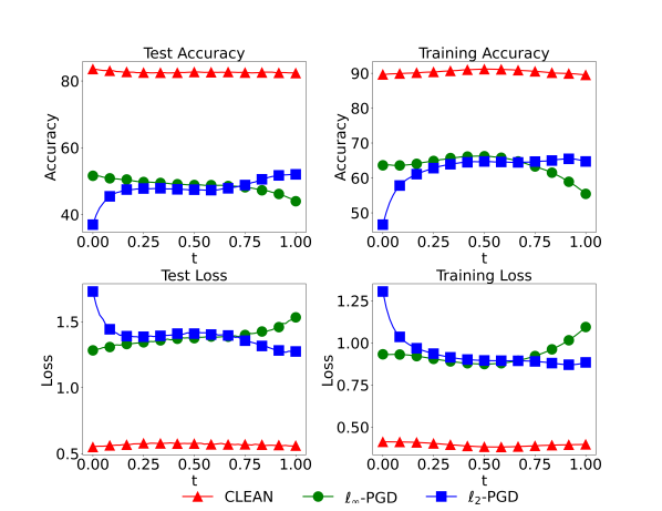
Figure 9: RMC-based optimization considering two types of perturbations (one single mid-optimal point) can result in paths with smoother and higher DLR than the path in Figure 4 left panel. The left (right) endpoint is an $\ell_{\infty}$-AT ($\ell_{2}$-AT) trained model starting from a single optimal point of a path connected between two models, which are trained by $\ell_{\infty}$-AT and $\ell_{2}$-AT for 50 epochs.

6.3 Robust Mode Connectivity-Based Optimization

As introduced in Section 5, Phase II of the Robust Mode Connectivity-Oriented Adversarial Defense is an enhanced optimization process based on units of RMC (Phase I). We show the effectiveness of RMC-based optimization (Phase II) below. Training epochs for all the experiments below are 200 (allow parallel computing).

Optimization on two types of perturbations. We first consider $\ell_{\infty}$ and $\ell_{2}$ norm perturbations. We train two models for 50 epochs under these two types of perturbations, then leverage RMC to find a path between the two models. Initializing from a single optimal point (randomly select from $t\in[0.77,0.83]$) on the curve, we train two models parallelly with $\ell_{\infty}$-AT and $\ell_{2}$-AT for 50 epochs. Finally, we plot the mode connectivity curve based on the two AT-trained models, as shown in Figure 9. We obtain a smoother path with higher DLR than the path in Figure 4 left panel. The optimal point achieved in this optimization process is $48.8\%$ at $t=0.72$.

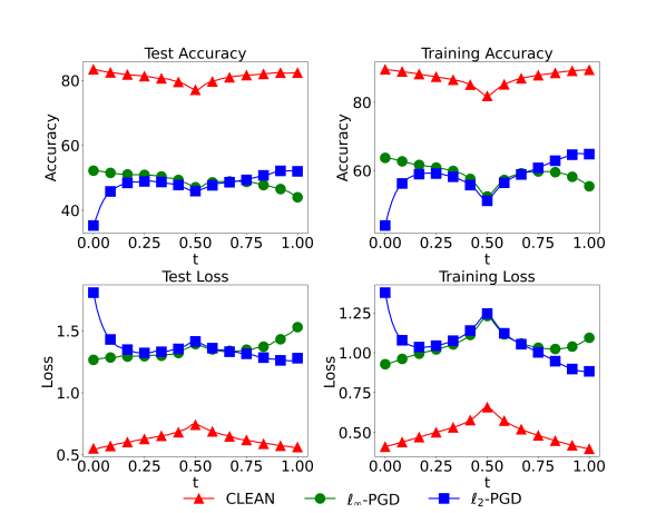
Figure 10: RMC-based optimization considering two types of perturbations with two mid-optimal points is able to achieve higher robustness compared with only selecting a single mid-optimal point. The left (right) endpoint is an $\ell_{\infty}$-AT ($\ell_{2}$-AT) trained model starting from two optimal points of a path connected between two models, which are trained by $\ell_{\infty}$-AT and $\ell_{2}$-AT for 50 epochs.

Now instead of selecting a single optimal point, we randomly pick two optimal points in the ranges of $t\in[0.27,0.33]$ and $t\in[0.77,0.83]$, respectively. We train two models with $\ell_{\infty}$-AT and $\ell_{2}$-AT for 50 epochs starting from each initial point. We then plot the RMC curve based on the two AT-trained models, as shown in Figure 10. The optimal point achieved in this optimization process is 48.89% (DLR) at $t=0.71$, indicating that higher robustness can be improved by using a larger population with higher diversity.

Optimization on three types of perturbations. We take one more step by considering the $\ell_{1}$ norm perturbation. The process is shown in Algorithm 2. $T=50$ and we use 50 additional epochs to learn RMC. The results of the final connection are shown in Fig. 11. The trend of the $\ell_{1}$-PGD curve is increasing from left to right and the trend of the $\ell_{2}$-PGD curve from $t=0.7$ to $t=1$ is decreasing. There exists an optimal point with DLR$=46.21\%$ at $t=0.93$. RMC-based optimization in the case of three types of perturbations can further boost models’ DLR against $\ell_{\infty}$, $\ell_{1}$, $\ell_{2}$ adversarial attacks.

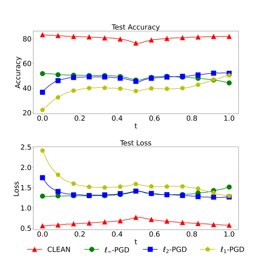
Figure 11: RMC-based optimization considering three types of perturbations can further boost models’ DLR against more types of attacks. The two endpoints are trained by $\ell_{\infty}$-AT and $\ell_{2}$-AT for 50 epochs starting from the optimal points selected from two RMC curves.

6.4 RMC-Based Optimization with SRMC Modules

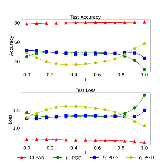
Figure 12: RMC-based optimization with SRMC modules considering three types of perturbations can find points with high DLR. SRMC modules can accelerate the speed of RMC-based optimization and saves computational cost.

We then test the proposed SRMC modules to speed up the process of RMC-based optimization. Starting from a $\ell_{\infty}$-AT model, an additional 5 epochs are used to train a $\ell_{2}$-AT model and a $\ell_{1}$-AT model. Then we connect each of the child models with the original $\ell_{\infty}$-AT model. Results are shown in Fig. 15 and Fig. 16 in Section 6.6. One can see that there exist paths with high-robustness regions under two connections. The results indicate that we do not need to train all the models from scratch to achieve desired paths.

Now we conduct the RMC-based optimization with SRMC modules on three types of perturbations. The pipeline is the same as the RMC-based optimization, except that we use self-generated $\ell_{2}$ and $\ell_{1}$ models as endpoints. As shown in Fig. 12, there exists an optimal point with DLR$=46.10\%$ at $t=0.82$. Compared with Fig. 11, optimization with SRMC achieves a similar level of DLR in a more efficient way.

TABLE I: Our Methods Can Achieve State-Of-Art DLR Level Under Different Perturbations. For methods using two types of perturbations, we only compare them using DLR under $\ell_{\infty}$-PGD and $\ell_{2}$-PGD attacks and mark the DLR (the lowest accuracy) using underline. For methods using three types of perturbations, we compare them on all metrics and mark the DLR (the lowest accuracy) under three basic $\ell_{p}$ attacks using overline. The baselines ($\ell_{\infty}$-AT [6] and MSD [14]) are all trained with 200 epochs. Our RMC with $\ell_{\infty}$ and $\ell_{2}$ norm perturbations is trained with 150 epochs’ endpoints and 50 epochs’ path search. All the RMC-based optimizations are trained with two RMC stages with each stage including 50 epochs’ endpoints and 50 epochs’ path searching. One can also see that our methods achieve the highest accuracy under Union and MSD.

	Standard Accuracy	$\ell_{\infty}$-PGD ($\delta=8/255$)	$\ell_{2}$-PGD ($\delta=1$)	$\ell_{1}$-PGD ($\delta=12$)	DLR	Union	MSD
$\ell_{\infty}$-AT	85.00%	49.03%	29.66%	16.61%	/	21.85%	15.27%
MSD (two types of pert)	81.61%	48.57%	45.92%	35.64%	45.92%	34.37%	45.72%
RMC (ours, two types of pert)	80.90%	48.19%	48.63%	38.05%	48.19%	36.3%	46.52%
RMC-based optimization (ours, two types of pert)	81.36%	48.89%	49.03%	38.83%	48.89%	36.86%	47.18%
MSD (three types of pert)	81.35%	$\overline{40.14\%}$	48.58%	47.50%	40.14%	38.35%	38.20%
RMC-based optimization (ours, three types of pert)	81.76%	$\overline{46.21\%}$	51.86%	46.23%	46.21%	41.47%	44.75%
RMC-based optimization with SRMC modules (ours, three types of pert)	80.39%	$\overline{46.10\%}$	48.92%	46.39%	46.10%	42.03%	45.07%

6.5 A Comprehensive Comparison

A comprehensive comparison is presented in Table I. We compared our proposed RMC (Phase I) and RMC-based optimization (Phase II) frameworks with a $\ell_{\infty}$-AT baseline [6] and the state-of-the-art method MSD [14]. All baselines were trained for 200 epochs. For MSD, RMC, and RMC-based optimization considering only two types of perturbations, we compared them under $\ell_{\infty}$-PGD and $\ell_{2}$-PGD attacks since we did not consider $\ell_{1}$-PGD attack during the training. The DLR (the lowest robust accuracy) under these two attacks is marked using underline. For methods using three types of perturbations, we compared them under $\ell_{\infty}$-PGD, $\ell_{2}$-PGD, $\ell_{\infty}$-PGD, MSD attacks, and the union metric. The DLR (the lowest robust accuracy) under $\ell_{\infty}$-PGD, $\ell_{2}$-PGD, $\ell_{\infty}$-PGD attacks are marked using overline. We also highlighted the highest accuracy in the union and MSD columns.

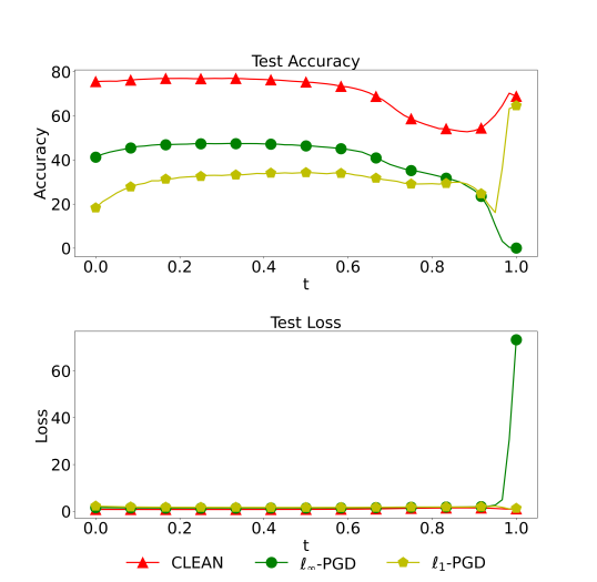
Figure 13: Curves obtained from two models trained by $\ell_{1}$-AT and $\ell_{\infty}$-AT contain points with higher DLR on $\ell_{1}$ and $\ell_{\infty}$-PGD attacks. The two endpoints are trained for 50 epochs.

From the table, it can be observed that: (1) RMC with two types of perturbations outperforms MSD with two types of perturbations by $2.27\%$ ($48.19\%-45.92\%$); (2) RMC-based optimization with two types of perturbations achieves slightly higher DLR than RMC and outperforms RMC on all other metrics; (3) RMC-based optimization with three types of perturbations outperforms MSD with three types of perturbations on DLR by $6.07\%$ and has higher accuracy on all metrics (except for $\ell_{1}$-PGD, where it is slightly lower than MSD); (4) The RMC-based optimization with SRMC modules can achieve similar (slightly lower) DLR performance compared to the RMC-based optimization with three types of perturbations, and even has slightly higher accuracy on the Union metric.

In conclusion, the two phases of the proposed Robust Mode Connectivity-Oriented Adversarial Defense demonstrate superior performance in various metrics, and RMC-based optimization (Phase II) achieves higher DLR than RMC (Phase I) alone. Overall, Robust Mode Connectivity-Oriented Adversarial Defense provides a new defense regime from a population-based optimization perspective and effectively enhances robustness in NNs.

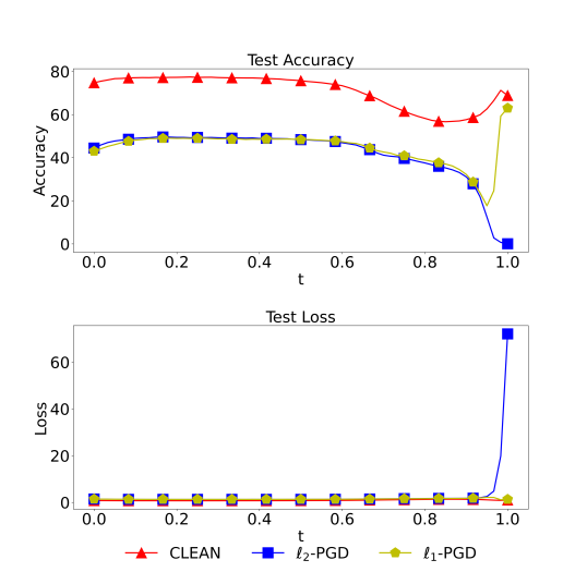
Figure 14: Curves obtained from two models trained by $\ell_{1}$-AT and $\ell_{2}$-AT contain points with higher DLR on $\ell_{1}$ and $\ell_{2}$-PGD attacks. The two endpoints are trained for 50 epochs.

6.6 Additional Results on RMC and SRMC

In Fig. 13 and Fig. 14, we show additional results of using RMC to find paths connecting a $\ell_{1}$-AT trained model and a $\ell_{\infty}$-AT ($\ell_{2}$-AT) trained model. Different from Fig. 6 and Fig. 7, here the two endpoints are trained for 50 epochs. One can find that the DLR is high even the number of training epochs is small. This ensures that under the scenario of using a small number of training epochs, we can still find good candidates to serve as new initial points in RMC-based optimization.

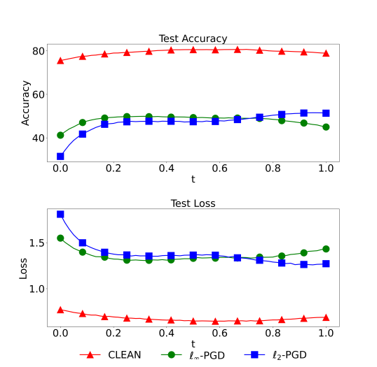
Figure 15: A single SRMC module can also find paths with high DRL by connecting a $\ell_{\infty}$ model and a $\ell_{2}$ model.

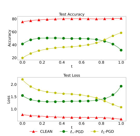
Figure 16: A single SRMC module can also find paths with high DRL by connecting a $\ell_{\infty}$ model and a $\ell_{1}$ model.

Fig. 15 and Fig. 16 show that a single SRMC module can also find paths with high DRL. The base model is trained by $\ell_{\infty}$-AT with 50 epochs. It serves as one endpoint. Starting from the base model, two models are trained by $\ell_{2}$-AT and $\ell_{1}$-AT with additional 5 epochs. They serve as the other endpoint. Fig. 15 shows the path connecting the $\ell_{\infty}$ model and the $\ell_{2}$ model. Fig. 16 shows the path between the $\ell_{\infty}$ model and the $\ell_{1}$ model.

7 Conclusion

In this paper, we propose a novel Robust Mode Connectivity-Oriented Adversarial Defense that can defend against diversified $\ell_{p}$ norm attacks and improve upon existing works using a population-based optimization strategy. We first introduce a new method called Robust Mode Connectivity (RMC), which corresponds to Phase I of the defense. RMC can discover a high-robustness path that connects two adversarially trained models against perturbations constrained on diversified $\ell_{p}$ norms. This approach enhances the Diversified $\ell_{p}$ Robustness (DLR) of neural networks and can be implemented as a defense method alone. We build on this method to develop Phase II of the defense, which is a multi-stage RMC-based population-based optimization regime that further boosts the DLR. To improve computational efficiency, we propose incorporating the Self-Robust Mode Connectivity (SRMC) module into the RMC-based optimization.

In addition, we conduct a comprehensive study of the RMC and RMC-based optimization methods and show that they can achieve significantly higher DLR than the baselines. Our findings demonstrate the effectiveness of the proposed methods in achieving high DLR against diversified $\ell_{p}$ threats, including $\ell_{\infty}$, $\ell_{2}$, $\ell_{1}$, and hybrid attacks. Our results show the potential of these methods for practical applications in real-world scenarios where the safety and security of machine learning systems are critical.

Ren Wang is an assistant professor in the Department of Electrical and Computer Engineering at the Illinois Institute of Technology, where he leads the Trustworthy and Intelligent Machine Learning (TIML) Research Lab. He received his bachelor’s degree and master’s degree in Electrical Engineering from Tsinghua University, Beijing, China, in 2013 and 2016. He received his Ph.D. degree in Electrical Engineering from Rensselaer Polytechnic Institute, Troy, NY, USA, in 2020. He was a postdoctoral research fellow in the Department of Electrical Engineering and Computer Science at the University of Michigan. His research interests include Trustworthy Machine Learning, High-Dimensional Data Analysis, Bio-Inspired Machine Learning, and Smart Grids.

Yuxuan Li is currently a graduate research intern at the Trustworthy and Intelligent Machine Learning Research Lab in the Department of Electrical and Computer Engineering, Illinois Institute of Technology. He is also pursuing his master’s degree at the Harbin Institute of Technology. He received his bachelor’s degree in Computer Science and Technology from Harbin Institute of Technology in 2021.

Sijia Liu received the Ph.D. degree (with the All University Doctoral Prize) in Electrical and Computer Engineering from Syracuse University, Syracuse, NY, USA, in 2016. He was a Postdoctoral Research Fellow at the University of Michigan, Ann Arbor, in 2016-2017, and a Research Staff Member at the MIT-IBM Watson AI Lab in 2018-2020. His research interests include scalable and trustworthy AI, e.g., adversarial deep learning, optimization theory and methods, computer vision, and computational biology. He received the Best Student Paper Award at the 42nd IEEE International Conference on Acoustics, Speech and Signal Processing (ICASSP). His work has been published at top-tier AI conferences such as NeurIPS, ICML, ICLR, CVPR, and AAAI.

References

- [1] D. Sarvamangala and R. V. Kulkarni, “Convolutional neural networks in medical image understanding: a survey,” Evolutionary intelligence, vol. 15, no. 1, pp. 1–22, 2022.
- [2] O. JiWei, L. C. TAY, and W. K. LAI, “Bottom-hat filtering for defect detection with cnn classification on car wiper arm,” in 2019 IEEE 15th International Colloquium on Signal Processing & Its Applications (CSPA), pp. 90–95, IEEE, 2019.
- [3] W. Li, D. Deka, R. Wang, and M. R. A. Paternina, “Physics-constrained adversarial training for neural networks in stochastic power grids,” IEEE Transactions on Artificial Intelligence, 2023.
- [4] I. J. Goodfellow, J. Shlens, and C. Szegedy, “Explaining and harnessing adversarial examples,” arXiv preprint arXiv:1412.6572, 2014.
- [5] R. Wang, T. Chen, P. Yao, S. Liu, I. Rajapakse, and A. O. Hero, “Ask: Adversarial soft k-nearest neighbor attack and defense,” IEEE Access, vol. 10, pp. 103074–103088, 2022.
- [6] A. Madry, A. Makelov, L. Schmidt, D. Tsipras, and A. Vladu, “Towards deep learning models resistant to adversarial attacks,” in International Conference on Learning Representations, 2018.
- [7] N. Carlini and D. Wagner, “Towards evaluating the robustness of neural networks,” in IEEE Symposium on Security and Privacy (SP), pp. 39–57, IEEE, 2017.
- [8] H. Zhang, Y. Yu, J. Jiao, E. P. Xing, L. E. Ghaoui, and M. I. Jordan, “Theoretically principled trade-off between robustness and accuracy,” International Conference on Machine Learning, 2019.
- [9] A. Shafahi, M. Najibi, M. A. Ghiasi, Z. Xu, J. Dickerson, C. Studer, L. S. Davis, G. Taylor, and T. Goldstein, “Adversarial training for free!,” in Advances in Neural Information Processing Systems, pp. 3353–3364, 2019.
- [10] R. Wang, K. Xu, S. Liu, P.-Y. Chen, T.-W. Weng, C. Gan, and M. Wang, “On fast adversarial robustness adaptation in model-agnostic meta-learning,” in International Conference on Learning Representations, 2020.
- [11] F. Tramer and D. Boneh, “Adversarial training and robustness for multiple perturbations,” Advances in Neural Information Processing Systems, vol. 32, 2019.
- [12] F. Croce and M. Hein, “Provable robustness against all adversarial -perturbations for ,” in International Conference on Learning Representations, 2019.
- [13] D. Stutz, M. Hein, and B. Schiele, “Confidence-calibrated adversarial training: Generalizing to unseen attacks,” in International Conference on Machine Learning, pp. 9155–9166, PMLR, 2020.
- [14] P. Maini, E. Wong, and Z. Kolter, “Adversarial robustness against the union of multiple perturbation models,” in International Conference on Machine Learning, pp. 6640–6650, PMLR, 2020.
- [15] F. Croce and M. Hein, “Adversarial robustness against multiple and single -threat models via quick fine-tuning of robust classifiers,” in International Conference on Machine Learning, pp. 4436–4454, PMLR, 2022.
- [16] J. Wang, T. Zhang, S. Liu, P.-Y. Chen, J. Xu, M. Fardad, and B. Li, “Adversarial attack generation empowered by min-max optimization,” Advances in Neural Information Processing Systems, vol. 34, pp. 16020–16033, 2021.
- [17] A. E. Eiben and J. Smith, “From evolutionary computation to the evolution of things,” Nature, vol. 521, no. 7553, pp. 476–482, 2015.
- [18] A. Díaz-Manríquez, G. Toscano, J. H. Barron-Zambrano, and E. Tello-Leal, “A review of surrogate assisted multiobjective evolutionary algorithms,” Computational intelligence and neuroscience, vol. 2016, 2016.
- [19] S. Mirjalili, “Evolutionary algorithms and neural networks,” in Studies in computational intelligence, vol. 780, Springer, 2019.
- [20] C. D. Freeman and J. Bruna, “Topology and geometry of half-rectified network optimization,” 2016.
- [21] T. Garipov, P. Izmailov, D. Podoprikhin, D. P. Vetrov, and A. G. Wilson, “Loss surfaces, mode connectivity, and fast ensembling of dnns,” Advances in neural information processing systems, vol. 31, 2018.
- [22] M. Jaderberg, V. Dalibard, S. Osindero, W. M. Czarnecki, J. Donahue, A. Razavi, O. Vinyals, T. Green, I. Dunning, K. Simonyan, et al., “Population based training of neural networks,” arXiv preprint arXiv:1711.09846, 2017.
- [23] X. Cui, W. Zhang, Z. Tüske, and M. Picheny, “Evolutionary stochastic gradient descent for optimization of deep neural networks,” Advances in neural information processing systems, vol. 31, 2018.
- [24] R. Wang, T. Chen, S. M. Lindsly, C. M. Stansbury, A. Rehemtulla, I. Rajapakse, and A. O. Hero, “Rails: A robust adversarial immune-inspired learning system,” IEEE Access, vol. 10, pp. 22061–22078, 2022.
- [25] P. Zhao, P.-Y. Chen, P. Das, K. N. Ramamurthy, and X. Lin, “Bridging mode connectivity in loss landscapes and adversarial robustness,” in International Conference on Learning Representations.
- [26] R. T. Farouki, “The bernstein polynomial basis: A centennial retrospective,” Computer Aided Geometric Design, vol. 29, no. 6, pp. 379–419, 2012.
- [27] J. Gomes, L. Velho, and M. C. Sousa, Computer graphics: theory and practice. CRC Press, 2012.
- [28] K. He, X. Zhang, S. Ren, and J. Sun, “Identity mappings in deep residual networks,” in European conference on computer vision, pp. 630–645, Springer, 2016.
- [29] R. Wang, T. Chen, S. Lindsly, C. Stansbury, I. Rajapakse, and A. Hero, “Immuno-mimetic deep neural networks (immuno-net),” The 2021 ICML Workshop on Computational Biology, 2021.
- [30] A. Krizhevsky and G. Hinton, “Learning multiple layers of features from tiny images,” Master’s thesis, Department of Computer Science, University of Toronto, 2009.