Statistical inference for association studies in the presence of binary outcome misclassification

Abstract

In biomedical and public health association studies, binary outcome variables may be subject to misclassification, resulting in substantial bias in effect estimates. The feasibility of addressing binary outcome misclassification in regression models is often hindered by model identifiability issues. In this paper, we characterize the identifiability problems in this class of models as a specific case of “label switching” and leverage a pattern in the resulting parameter estimates to solve the permutation invariance of the complete data log-likelihood. Our proposed algorithm in binary outcome misclassification models does not require gold standard labels and relies only on the assumption that outcomes are correctly classified at least 50% of the time. A label switching correction is applied within estimation methods to recover unbiased effect estimates and to estimate misclassification rates. Open source software is provided to implement the proposed methods. We give a detailed simulation study for our proposed methodology and apply these methods to data from the 2020 Medical Expenditure Panel Survey (MEPS).

Keywords: association studies, bias correction, EM algorithm, identification, label switching, MCMC

1 Introduction

We consider regression models where a binary outcome variable is potentially misclassified. Misclassified binary outcomes are common in biomedical and public health association studies. For example, misclassification may occur in when a diagnostic test does not have perfect sensitivity or specificity ^{1, 2, 3}. Misclassification can also be present in survey data, where individuals may falsely recall disease status on a self-report item ⁴. More recently, medical studies may rely on computer algorithms to extract patient disease status from electronic medical records, but such algorithms do not perfectly capture true disease states, even when combined with record review from subject-area experts ⁵. It is common for analysts to ignore potential misclassification in response variables, and instead assume that the outcome is perfectly measured. Such an approach generally produces biased parameter estimates ⁶, particularly in the case of covariate-related misclassification ⁷, ⁸.

Despite the known impact of covariate-related misclassification, previous work on recovering unbiased association parameters is limited. Neuhaus⁹ provides general expressions for bias in the presence of covariate-related misclassification. Lyles et al. ¹⁰ and Lyles and Lin¹¹ extend this work, but require a validation sample or known sensitivity and specificity values, respectively, to identify association parameters. Beesley and Mukherjee ⁷ address the problem through a novel likelihood-based bias correction strategy, but make the strong assumption that the binary outcome is measured with perfect specificity. A perfect specificity assumption also underpins existing sensitivity analysis frameworks for evaluating the predictive bias of classifiers in the presence of outcome misclassification ¹². Zhang and Yi⁸ develop methods to correct bias in association parameters in the context of covariate-related misclassification, but they only address the problem for mixed continuous and binary bivariate outcomes. Our methods consider scenarios where validation data is not available, but the binary outcome is subject to covariate-dependent, bidirectional misclassification.

Numerous researchers instead assume that sensitivity and specificity may be considered constant ¹³, ¹⁴, ³, ¹⁵, ¹⁶, ¹⁷, ¹⁸. In such cases, misclassification rates are often either assumed to be known ¹³, ³ or estimated via validation data ¹⁶, ¹⁵. In the event that an outcome measure has previously studied sensitivity and specificity rates, as is common for commercially available diagnostic tests, EM algorithm methods exist to incorporate that information into the fitting of logistic regression models, resulting in unbiased estimates of odds ratios ¹³. For cases where internal validation data are present, Carroll and colleagues ¹⁵ develop general expressions for likelihood functions that take imperfect outcome measurement into account. These methods rely on the availability of gold standard measures, which are not feasible in numerous biomedical and public health settings ¹⁹, ²⁰. In contrast, fully Bayesian methods may be used to estimate constant misclassification rates in the absence of a gold standard, but such methods rely on strict and difficult prior elicitation strategies ¹⁴, ¹⁸ or an additional assumption of equal sensitivity and specificity ²¹, ²².

The impact of misclassification has also been considered for estimates of outcome prevalence. Econometricians have used partial identifiability to address misclassification and estimate population rates of SARS CoV-2 infection ²³, ¹, but these methods do not readily extend to association studies. Misclassification can also impact variance estimation in prevalence studies. Ge et al. ² derive an estimable variance component that is induced by misclassification in certain testing applications, but their methods also rely on known sensitivity and specificity rates.

In the machine learning literature, the problem of outcome misclassification, or “noisy labels”, is typically handled with noise-robust methods or data cleaning strategies ²⁴. Other methods approach misclassification from a fairness lens, where an optimization approach is proposed to “flip” predicted labels after estimation to alleviate systematic bias without sacrificing the value of “merit” within the classification scheme ²⁵. When imperfect classification algorithms are used to obtain disease states, Sinnott and colleagues ⁵ demonstrate that modeling outcome probabilities, rather than outcomes obtained via thresholding, improves power and estimation accuracy.

In this paper, we develop new strategies to recover unbiased parameter estimates in association studies with outcome misclassification that is related to observed covariates. We propose a bias correction strategy that requires minimal external information, no gold standard labels, and no limitations on the misclassification patterns present in the data.

The feasibility of addressing outcome misclassification in association studies is often limited by model identifiability issues ¹⁰, ²⁶. One aspect of model identifiability that must be addressed for a binary outcome misclassification model is the phenomenon of “label switching”. Label switching describes the invariance of the likelihood under relabeling of the mixture components, resulting in multimodal likelihood functions ²⁷. Several remedies have been suggested to break the permutation invariance of the likelihood in both Bayesian and frequentist mixture models ²⁸, ²⁹. One common method is to impose ordering constraints on component model parameters, such as $\pi_{1}<\pi_{2}$ ³⁰. Such strategies aim to remove the permutation invariance of the likelihood, but are only successful for carefully chosen constraints ³¹. In Bayesian settings, one potential resolution of the labeling degeneracy is to use non-exchangeable prior distributions to strongly separate possible parameter sets ³⁰. It is rare, however, that analysts have enough information to set useful ordering constraints or strongly separated prior distributions in practice ²⁸. Moreover, when prior distributions for sensitivity and specificity are misspecified, bias correction approaches tend to perform poorly ³², ¹⁴. As such, we develop a novel label switching remedy that relies only on the reasonable assumption that correct outcome classification occurs in at least $50\%$ of observations.

We use our label switching correction procedure to develop both frequentist and Bayesian estimation methods for regression parameters in an association study. This strategy also allows us to accurately estimate the average misclassification rates in the response variable and characterize the mechanism by which misclassification occurs.

In addition to label switching, several authors have considered other characteristics of misclassification models that impact identifiability. Xia and Gustafson ¹⁷ outlines cases of unidirectional outcome misclassification where key regression parameters are identifiable. In many practical settings, however, they find that some covariate terms can only be weakly identified. Numerical problems related to weak identifiability are also encountered the joint estimation methods by Beesley and Mukherjee ⁷. These authors address the problem by fixing model parameters at known values. In general, however, models that include a parametric observation mechanism for misclassified outcomes are identifiable if 1) perfect sensitivity or perfect specificity is assumed and 2) at least one continuous covariate is included in the true outcome mechanism but not the observation mechanism, or vice versa ^{7, 33}. For models that do not have covariate-dependent misclassification rates, global identifiability of univariate logistic regression with outcome misclassification is ensured if at least four values of the covariate are observed and the true regression coefficient in the model is non-zero ²⁶. For misclassification models that fall into the larger class of finite mixtures of logistic regressions, as our proposed framework does, identifiability is guaranteed as long as there is a sufficient number of unique observed covariate combinations ³⁴. If the mixture has two components, this sufficient number of covariates is just seven ^{34, 35}. Throughout this paper, we will assume that this criterion for identification is met.

In Section 2, we describe the conceptual framework for our model. Section 3 describes the label switching problem in greater detail and proposes a strategy to break permutation invariance of the likelihood in a binary outcome misclassification model. In Section 4, we propose frequentist and Bayesian estimation strategies to recover the true association of interest in the presence of potentially misclassified observed outcomes. For all strategies proposed, we provide software for implementation using the R package COMBO (COrrecting Misclassified Binary Outcomes). Through simulation, we demonstrate the utility of these methods to reduce bias in parameter estimates when compared to analyses that place restrictions on or ignore outcome misclassification. Finally, we apply our proposed methods to investigate am applied example. In particular, we study risk factors for myocardial infarction, which is known to be misdiagnosed on the basis of gender and age ³⁶, ³⁷, ³⁸.

2 Model, Notation, and Conceptual Framework

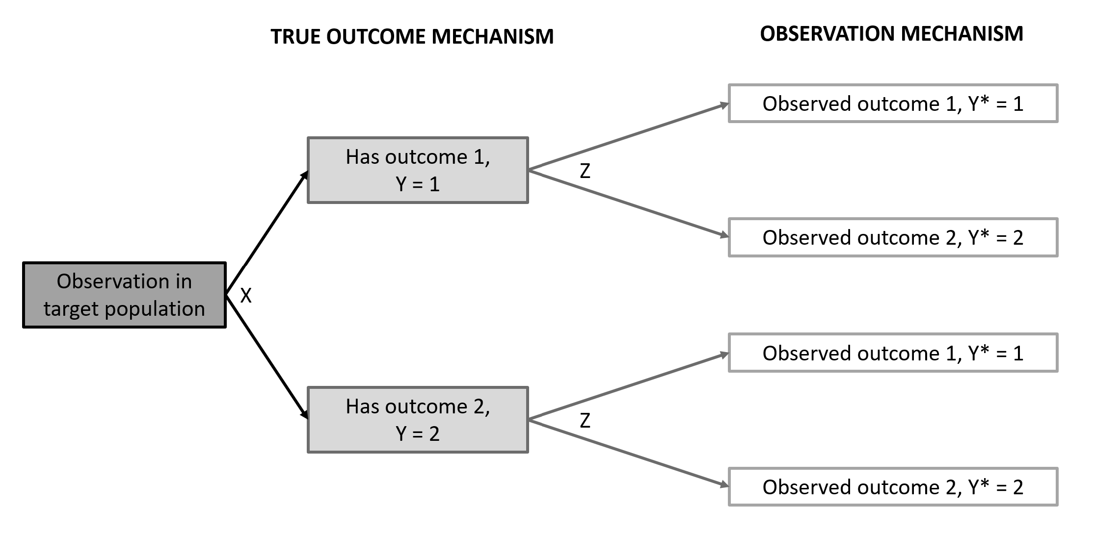
Figure 1: Diagram of the assumed data structure for a binary outcome misclassification model.

Let $Y=j$ denote an observation’s true outcome status, taking values $j\in\{1,2\}$. Suppose we are interested in the relationship between $Y$ and a set of predictors, $X$, that are correctly measured. This relationship constitutes the true outcome mechanism. Let $Y^{*}=k$ be the observed outcome status, taking values $k\in\{1,2\}$. $Y^{*}$ is a potentially misclassified version of $Y$. Let $Z$ denote a set of predictors related to sensitivity and specificity. The mechanism that generates the observed outcome, $Y^{*}$, given the true outcome, $Y$, is called the observation mechanism. Figure 1 displays the conceptual model. The conceptual process is mathemathically expressed as

True outcome mechanism: $$\;\operatorname{logit}\{P(Y=j|X;\beta)\}=\beta_{j0}+\beta_{jX}X$$ (1)

Observation mechanism: $$\;\operatorname{logit}\{P(Y^{*}=k|Y=j,Z;\gamma)\}=\gamma_{kj0}+\gamma_{kjZ}Z.$$

In the true outcome mechanism, we use category $Y=2$ as the reference category, and set all corresponding $\beta$ parameters to 0. Similarly, $Y^{*}=2$ is the reference category in the observation mechanism, and all corresponding $\gamma$ parameters are also set to 0. Using (1), we can express response probabilities for individual $i$’s true outcome category and for individual $i$’s observed category, conditional on the true outcome:

$$\begin{aligned} P(Y_{i}=j|X;\beta)=&\;\;\pi_{ij}=\frac{\text{exp}\{\beta_{j0}+\beta_{jX}X_{i}\}}{1+\text{exp}\{\beta_{j0}+\beta_{jX}X_{i}\}}\\ P(Y^{*}_{i}=k|Y_{i}=j,Z;\gamma)=&\;\pi^{*}_{ikj}=\frac{\text{exp}\{\gamma_{kj0}+\gamma_{kjZ}Z_{i}\}}{1+\text{exp}\{\gamma_{kj0}+\gamma_{kjZ}Z_{i}\}}.\end{aligned}$$ (2)

These quantities can be calculated for all $N$ observations in the sample. For $j$ and $k$ both equal to the reference category, $\sum_{i=1}^{N}\pi^{*}_{i22}=\pi^{*}_{22}$ measures the specificity in the data. When $j$ and $k$ are both $1$, $\sum_{i=1}^{N}\pi^{*}_{i11}=\pi^{*}_{11}$ measures the sensitivity. Thus, (2) allows us to model sensitivity and specificity based on a set of covariates, $Z$. It is common for analysts to ignore potential misclassification in $Y^{*}$, and instead to use a naive analysis model $Y^{*}|X$ and interpret the results under the true outcome model $Y|X$. Previous work has shown that this approach produces bias in $P(Y^{*}=j|X)$ relative to $P(Y=j|X)$, particularly in the case of covariate-related misclassification ⁷.

We define the probability of observing outcome $k$ using the model structure as

$$P(Y^{*}=k|X,Z)=\sum_{j=1}^{2}P(Y^{*}=k|Y=j,Z;\gamma)P(Y=j|X;\beta)=\sum_{j=1}^{2}\pi^{*}_{kj}\pi_{j}.$$ (3)

The contribution to the likelihood by a single subject $i$ is thus $\prod_{k=1}^{2}P(Y^{*}_{i}=k|X_{i},Z_{i})^{y^{*}_{ik}}$ where $y^{*}_{ik}=\mathbbm{I}(Y^{*}_{i}=k)$ and where $\mathbbm{I}(A)$ is the indicator of the set $A$. We can estimate $(\beta,\gamma)$ using the following observed data log-likelihood for subjects $i=1\dots N$ as

$$\ell_{obs}(\beta,\gamma;X,Z)=\sum_{i=1}^{N}\sum_{k=1}^{2}y^{*}_{ik}\text{log}\{P(Y^{*}_{i}=k|X_{i},Z_{i})\}=\sum_{i=1}^{N}\sum_{k=1}^{2}y^{*}_{ik}\text{log}\{\sum_{j=1}^{2}\pi^{*}_{ikj}\pi_{ij}\}.$$ (4)

The observed data log-likelihood is difficult to use directly for estimation because jointly maximizing $\beta$ and $\gamma$ is numerically challenging, especially for large datasets.

Viewing the true outcome value $Y$ as a latent variable, we may also construct the complete data log-likelihood based on the model structure as

$$\ell_{complete}(\beta,\gamma;X,Z) =\sum_{i=1}^{N}\Bigg{[}\sum_{j=1}^{2}y_{ij}\text{log}\{P(Y_{i}=j|X_{i})\}+\sum_{j=1}^{2}\sum_{k=1}^{2}y_{ij}y^{*}_{ik}\text{log}\{P(Y^{*}_{i}=k|Y_{i}=j,Z_{i})\}\Bigg{]}$$ (5)

$$=\sum_{i=1}^{N}\Bigg{[}\sum_{j=1}^{2}y_{ij}\text{log}\{\pi_{ij}\}+\sum_{j=1}^{2}\sum_{k=1}^{2}y_{ij}y^{*}_{ik}\text{log}\{\pi^{*}_{ikj}\}\Bigg{]},$$

where $y_{ij}=\mathbbm{I}(Y_{i}=j)$. Without the true outcome value, $Y$, we cannot use this likelihood form directly for maximization. It is notable, however, that (5) can be viewed as a mixture model with latent mixture components, $y_{ij}$, and covariate-dependent mixing proportions, $\pi_{ij}$.

3 Label Switching

The structure of the models described in Section 2 suffers from the known problem of label switching in mixture likelihoods. Mixture likelihoods are invariant under relabeling of the mixture components, resulting in multimodal likelihood functions ²⁷. Specifically, a $J$-dimensional mixture model will have $J!$ modes in the likelihood ³⁰. Given that our proposed model in (5) is a mixture with $J=2$ components labeled by the true outcome $Y\in\{1,2\}$, there are $J!=2!=2$ peaks in the likelihood resulting in $2$ plausible parameter sets.

3.1 Permutation Invariance of the Complete Data Likelihood

The invariance of the complete data log-likelihood under relabeling of mixture components is displayed in (6) and (7). In (6), we label $Y$ terms in the order of appearance as either $1$ or $2$. In (7), all terms that had $Y=1$ are replaced with that of $Y=2$ and all terms that had $Y=2$ are replaced with $Y=1$. It follows that,

$$\ell_{complete}(\beta,\gamma;X,Z)= \sum_{i=1}^{N}\Bigl{[}y_{i1}\log\{\pi_{i1}\}+y_{i2}\log\{\pi_{i2}\}$$ (6)

$$\phantom{a}+y_{i1}y^{*}_{i1}\log\{\pi^{*}_{i11}\}+y_{i1}y^{*}_{i2}\log\{\pi^{*}_{i21}\}+y_{i2}y^{*}_{i1}\log\{\pi^{*}_{i12}\}+y_{i2}y^{*}_{i2}\log\{\pi^{*}_{i22}\}\Bigr{]},$$

$$\ell_{complete}(\beta,\gamma;X,Z)= \sum_{i=1}^{N}\Bigl{[}y_{i2}\log\{\pi_{i2}\}+y_{i1}\log\{\pi_{i1}\}$$ (7)

$$\phantom{a}+y_{i2}y^{*}_{i1}\log\{\pi^{*}_{i12}\}+y_{i2}y^{*}_{i2}\log\{\pi^{*}_{i22}\}+y_{i1}y^{*}_{i1}\log\{\pi^{*}_{i11}\}+y_{i1}y^{*}_{i2}\log\{\pi^{*}_{i21}\}\Bigr{]}.$$

Due to the additive structure of the complete data log-likelihood, the label change between (6) and (7) does not impact the value of the function. Thus, the complete data log-likelihood in our setting is invariant under relabeling of mixture components.

Suppose for each $y_{ij}$ we have a single predictor $x_{i}$ in the true outcome mechanism and a single predictor $z_{i}$ in the observation mechanism. Substituting the parametric form of the response probabilities from (2) into (6) and (7), we can detect a pattern in the parameters associated with each likelihood mode, that is,

$$\sum_{i=1}^{N}\Bigl{[}y_{i1}\beta_{0}+y_{i1}x_{i}\beta_{X}-(y_{i1}+y_{i2})\log\{1+\exp\{\beta_{0}+x_{i}\beta_{X}\}\}$$ (8)

$$\qquad\phantom{a}+y_{i1}y^{*}_{i1}\gamma_{110}+y_{i1}y^{*}_{i1}z_{i}\gamma_{11Z}-(y^{*}_{i1}+y^{*}_{i2})y_{i1}\log\{1+\exp\{\gamma_{110}+z_{i}\gamma_{11Z}\}\}$$

$$\qquad\phantom{a}+y_{i2}y^{*}_{i1}\gamma_{120}+y_{i2}y^{*}_{i1}z_{i}\gamma_{12Z}-(y^{*}_{i1}+y^{*}_{i2})y_{i2}\log\{1+\exp\{\gamma_{120}+z_{i}\gamma_{12Z}\}\}\Bigr{]}$$

$$= \sum_{i=1}^{N}\Bigl{[}y_{i2}(-\beta_{0})+y_{i2}x_{i}(-\beta_{X})-(y_{i1}+y_{i2})\log\{1+\exp\{-\beta_{0}+x_{i}(-\beta_{X})\}\}$$

$$\qquad\phantom{a}+y_{i2}y^{*}_{i1}\gamma_{120}+y_{i2}y^{*}_{i1}z_{i}\gamma_{12Z}-(y^{*}_{i1}+y^{*}_{i2})y_{i2}\log\{1+\exp\{\gamma_{120}+z_{i}\gamma_{12Z}\}\}$$

$$\qquad\phantom{a}+y_{i1}y^{*}_{i1}\gamma_{110}+y_{i1}y^{*}_{i1}z_{i}\gamma_{11Z}-(y^{*}_{i1}+y^{*}_{i2})y_{i1}\log\{1+\exp\{\gamma_{110}+z_{i}\gamma_{11Z}\}\}\Bigr{]}.$$

Specifically, label switching generates the following two parameter sets: (1) $\beta_{0},\beta_{X},\gamma_{110},\gamma_{11Z},\gamma_{120},\gamma_{12Z}$, and (2) $-\beta_{0},-\beta_{X},\gamma_{120},\gamma_{12Z},\gamma_{110},\gamma_{11Z}$. Suppose the true values of each parameter were equal to real numbers $a,b,c,d,e,f$, respectively, for parameter set 1. The two parameter sets corresponding to these values would be: (1) $a,b,c,d,e,f$, and (2) $-a,-b,e,f,c,d$. That is, the $\beta$ parameters change signs while the $\gamma$ parameters change $j$ subscripts between the two parameter sets. This pattern is stable for any dimension of $x$ and $z$ vector predictors. In practice, if an analyst uses frequentist estimation methods, they will recover only one of the two parameter sets. When this model is fit via Gibbs Sampling, it is typical for different chains to center at different parameter sets. Moreover, each chain is generally unable to transition between modes within a finite running time ³⁰. Thus, it is possible for a final posterior sample to reflect estimates from different “label switched” parameter sets, making the results difficult to meaningfully summarize ³¹.

3.2 A Strategy to Correct Label Switching

Given that the two likelihood modes present in the proposed model are known, we now describe a method to select the correct parameter set. After obtaining parameter estimates $\hat{\beta}$ and $\hat{\gamma}$ from an estimation method described in Section 4, the appropriate parameter set, $\hat{\beta}_{corrected}$ and $\hat{\gamma}_{corrected}$, can be determined using the following algorithm.

Algorithm 1 Correcting label switching in binary outcome misclassification models

Compute average $\pi^{*}_{jj}$ for all $j\in\{1,2\}$ using $\hat{\beta}$ and $\hat{\gamma}$.

if $\pi^{*}_{jj}>0.50$ for all $j\in\{1,2\}$ then

     $\hat{\beta}_{corrected}\leftarrow\hat{\beta}$

     $\hat{\gamma}_{corrected}\leftarrow\hat{\gamma}$

else

     $\hat{\beta}_{corrected}\leftarrow-\hat{\beta}$

     $\hat{\gamma}_{corrected,k1}\leftarrow\hat{\gamma_{k2}}$

     $\hat{\gamma}_{corrected,k2}\leftarrow\hat{\gamma_{k1}}$

end if

Algorithm 1 relies on the following assumption:

Assumption 1

Within identified models, the probability of correct classification is at least 0.50, on average across subjects $i$; that is, $\pi^{*}_{jj}>0.50$.

Assumption 1 is required because it allows for differentiation between the two possible parameter sets for this model. As displayed in (6) and (7), each parameter set assigns a different category of the latent variable, $Y=1$ or $Y=2$, to each component of the mixture likelihood. This means that when we compute $\pi^{*}_{kj}=P(Y^{*}=k|Y=j)$ for a given observed outcome category, $k$, it is possible that $\pi^{*}_{kj}$ could refer to $\pi^{*}_{k1}$ or $\pi^{*}_{k2}$. In order to differentiate between these two latent variable assignments, we make the assumption that $\pi^{*}_{k=j,j}>\pi^{*}_{k\neq j,j}$ which implies $\pi^{*}_{k=j,j}>0.50$. Thus, we are able to determine which latent category labeling is more plausible in our results. Assumption 1 is reasonable because it assumes that the observation mechanism is at least as good as a coin flip, on average.

Such assumptions are not required in other methods like ⁷ and ¹⁷ because unidirectional misclassification is assumed. Thus, only one latent outcome category is present in the complete data log-likelihood and so the resulting functional form is not permutation invariant.

4 Estimation Methods

In this section, we describe two estimation methods for our proposed binary outcome misclassification model that exploit the latent variable structure of this problem. First, we propose jointly estimating $\beta$ and $\gamma$ using the expectation-maximization (EM) algorithm ³⁹. Next, we outline Bayesian methods for analyzing data from association studies in the presence of binary outcome misclassification. Both estimation strategies are available in the R package COMBO.

4.1 Maximization Using an EM Algorithm

We use the complete data log-likelihood as the starting point for the EM algorithm. Since (5) is linear in $y_{ij}$, we can replace $y_{ij}$ in the E-step of the EM algorithm with the quantity

$$w_{ij}=P(Y_{i}=j|Y_{i}^{*},X,Z)=\sum_{k=1}^{2}\frac{y^{*}_{ik}\pi^{*}_{ikj}\pi_{ij}}{\sum_{\ell=1}^{2}\pi^{*}_{ik\ell}\pi_{i\ell}}.$$ (9)

In the M-step, we maximize the expected log-likelihood with respect to $\beta$ and $\gamma$

$$Q=\sum_{i=1}^{N}\Bigl{[}\sum_{j=1}^{2}w_{ij}\text{log}\{\pi_{ij}\}+\sum_{j=1}^{2}\sum_{k=1}^{2}w_{ij}y^{*}_{ik}\text{log}\{\pi^{*}_{ikj}\}\Bigr{]}.$$ (10)

The $Q$ function in (10) can be split into three separate equations for estimating $\beta$ and $\gamma$

$$Q_{\beta}=\sum_{i=1}^{N}\Bigl{[}\sum_{j=1}^{2}w_{ij}\text{log}\{\pi_{ij}\}\Bigr{]},\>Q_{\gamma_{k1}}=\sum_{i=1}^{N}\Bigl{[}\sum_{k=1}^{2}w_{i1}y^{*}_{ik}\text{log}\{\pi^{*}_{ik1}\}\Bigr{]},\>Q_{\gamma_{k2}}=\sum_{i=1}^{N}\Bigl{[}\sum_{k=1}^{2}w_{i2}y^{*}_{ik}\text{log}\{\pi^{*}_{ik2}\}\Bigr{]}.$$ (11)

In practice, $Q_{\beta}$ in (11) can be fit as a logistic regression model where the outcome is replaced by weights, $w_{ij}$. $Q_{\gamma_{k1}}$ and $Q_{\gamma_{k2}}$ in (11) each are fit as weighted logistic regression models where the outcome is $y^{*}_{ik}$ ⁴⁰. After estimates for $\beta$ and $\gamma$ are obtained, Algorithm 1 is required to return final parameter estimates. The covariance matrix for $\beta$ and $\gamma$ is obtained by inverting the expected information matrix.

4.2 Bayesian Modeling

Our proposed binary outcome misclassification model is: $Y^{*}_{ik}|\pi^{*}_{ik}\sim Multinomial(\pi^{*}_{ik},J)$, where $\pi^{*}_{ik}=\sum_{j=1}^{2}\pi^{*}_{ikj}\pi_{ij}$ as in (3) and $J$ denotes the number of outcome categories (in this case, $2$).

Assumptions and prior distributions for the parameters are based on input from subject-matter experts on the data the model is applied to. It is recommended that prior distributions are proper and relatively flat to ensure model identifiability without strongly influencing the posterior mean estimation. For example, in cases where non-informative priors are desired, a Uniform prior with a wide range may be selected. If an analyst has previous data suggesting a plausible estimate for a given parameter, a Normal prior distribution with a wide variance that is centered at the previous estimate may be used. In the R Package, COMBO, analysts may select between Uniform, Normal, Double Exponential, or t prior distributions, with user-specified prior parameters. Before summarizing the results, Algorithm 1 should be applied on each individual MCMC chain, to address potential label switching within a given chain. Standard methods can be used to compute variance metrics.

5 Simulations

We present simulations for evaluating the proposed binary outcome misclassification model in terms of bias and root mean squared error (rMSE). Our methods are compared to the SAMBA R package and an adapted version of SAMBA where the observation mechanism is assumed to have either perfect specificity or perfect sensitivity, respectively. We also compare all methods that account for misclassification to a naive logistic regression that assumes there is no measurement error in the observed outcome.

The model simulation study includes three settings: (1) small sample size and large misclassification rates, (2) large sample size and small misclassification rates, and (3) moderate sample size with perfect specificity. Details on these settings can be found in Appendix A.

Figures 2 and 3 present the parameter estimates for Setting 1 and Setting 2, respectively, across 500 simulated datasets. Figure 4 presents parameter estimates under Setting 3. Table 1 presents mean parameter estimates and rMSE across 500 simulated datasets for each setting and estimation method. Table 2 presents the true outcome probability, sensitivity, and specificity values measured from the generated data and estimated from the EM algorithm and MCMC results for each simulation scenario.

Setting 1: Across all simulated datasets, the average $P(Y=1)$ was 64.7% and the average $P(Y^{*}=1)$ was 59.1% (Table 2). The average correct classification rate was 84.7% for $Y=1$ and 87.7% for $Y=2$. In Table 1, we see that the naive logistic regression analysis results in substantial bias the estimate of $\beta_{X}$. If only one type of misclassification is assumed using SAMBA EM or “Perfect Sensitivity EM”, bias in the estimated parameters is high. Our proposed EM Algorithm performs well for $\beta$ parameter estimates, but has wide variation in some $\gamma$ estimates. Similar results are observed for our propsed MCMC method. The rMSE in the parameter estimates is generally smaller when comparing the EM estimates to the MCMC estimates. The EM estimates also achieve lower rMSE than estimates from SAMBA EM and Perfect Sensitivity EM. Both the EM Algorithm and MCMC methods recover the true outcome probabilities $P(Y=1)$ and $P(Y=2)$, but MCMC tends to consistently overestimate the sensitivity and specificity values compared to the EM Algorithm (Table 2).

Setting 2: In Setting 2, the average $P(Y=1)$ was 64.7% and the average $P(Y^{*}=1)$ was 61.8% across all simulated datasets (Table 2). The average correct classification rate was 92.4% for $Y=1$ and 94.5% for $Y=2$. There is substantial bias in the estimate of $\beta_{X}$ in the naive logistic regression and perfect sensitivity EM results in Table 1. If perfect specificity is assumed in SAMBA EM, the bias in the estimate of $\beta_{X}$ is improved compared to the naive and perfect sensitivity cases, but is much higher than if both types of misclassification are accounted for. Our proposed EM Algorithm method performs well for $\beta$ and $\gamma$ parameter estimates. Similar results are observed for the proposed MCMC method, though bias in some $\gamma$ estimates is higher than that observed using the EM algorithm. The rMSE in the $\beta$ parameter estimates is comparable between the EM and MCMC methods. However, rMSE in the $\gamma$ parameter estimates is generally smaller for EM than MCMC. Both EM and MCMC estimates, however, achieve lower rMSE than estimates from the methods that make perfect sensitivity and/or specificity assumptions. In Table 2, we see that both the EM and MCMC methods recover the true outcome probabilities with virtually no bias. In addition, both methods achieve low bias in the estimation of $P(Y^{*}=1|Y=1)$ and $P(Y^{*}=2|Y=2)$.

Setting 3: In Setting 3, the average $P(Y=1)$ was 64.7% and the average $P(Y^{*}=1)$ was 54.8% (Table 2). Per the simulation design, there was no misclassification for $Y=2$. The average correct classification rate was 84.6% for $P(Y=1)$. In this setting, the naive analysis and perfect sensitivity methods return highly biased $\beta$ estimates (Table 1). There is also substantial bias in the $\gamma$ estimates for the perfect sensitivity EM method. This is unsurprising, since the $\gamma_{120}$ and $\gamma_{12Z}$ terms govern the specificity portion of the observation mechanism, which is error-free in this setting. The framework of Setting 3 matches the SAMBA EM method developed by Beesley and Mukherjee⁷, and it is unsurprising that low bias and rMSE is observed across all SAMBA EM parameter estimates. Despite making no assumptions on misclassification direction in a setting with perfect specificity, the proposed EM and MCMC parameter estimates have low bias for all $\beta$ terms and for $\gamma_{110}$ and $\gamma_{11Z}$. Substantial bias is observed in the EM case for $\gamma_{120}$ and $\gamma_{12Z}$. This bias is largely the result of extreme parameter estimates in some simulated datasets, as observed in Figure 4. Despite the extreme variation in the $\gamma_{120}$ and $\gamma_{12Z}$ estimates across simulations, the remaining parameters are estimated with low bias and with rMSE near that of the SAMBA EM estimates (Table 1). In the MCMC results for $\gamma_{120}$ and $\gamma_{12Z}$, we see much less bias and much smaller rMSE than the EM estimates. This behavior is likely due to the Uniform prior distribution, which limited the posterior samples to the $[-10,10]$ range. In Table 2, both the EM and MCMC methods return accurate estimates of $P(Y=1)$ and $P(Y=2)$. The EM method slightly overestimates sensitivity and slightly underestimates specificity. The MCMC method also slightly overestimates sensitivity, but correctly estimates perfect specificity in the datasets.

6 Applied Example

In this section, we perform a case study using data from the 2020 Medical Expenditure Panel Survey (MEPS), a sequence of surveys on cost and use of health care and health insurance status in the United States ⁴¹. We are primarily interested in risk factors associated with myocardial infarction (MI). This association, however, is potentially impacted by misclassification in self-reported history of MI. In particular, it is possible for the symptoms of other ailments to be attributed to MI and for the chest pain of MI to be attributed to a different diagnosis. These types of misdiagnoses are known to be more common in women than men ³⁶, ³⁷ and among younger patients ³⁸. Thus, we expect misclassification of self-reported history of MI to be associated with patient gender and age. Our overall goal is to assess the severity of this misclassification, and to understand the impact of misclassification on the association between risk factors and MI. The MEPS 2020 survey was used for this analysis because, at the time of writing, this was the most recently collected MEPS data. In addition, the disruption of the COVID-19 pandemic in the 2020 year may have contributed additional measurement error to medical diagnoses in the dataset ⁴¹.

Our response variable of interest is whether or not survey respondents reported any history of MI. We assessed the association of MI status with risk factors including age, smoking status, and exercise habits. The age variable was centered and scaled before use in the model. Smoking status and exercise variables were coded as binary indicators. The use of a continuous age variable ensures that we have at least seven unique covariate values in this setting. Thus, we have satisfied the conditions for identification of a finite mixture model with two mixture components.

For the analysis, we included data only from participants age 18-85. For each family unit recorded in the dataset, we only keep the responses of the reference person. After excluding all of the records with missing values in the response and covariates, we had a total of 12731 observations on our analysis. In this dataset, 640 (5%) reported a history of MI.

We estimate model parameters using the EM algorithm with label switching correction from Section 4.1. Parameter estimates and standard errors are reported in Table 3. The $\beta$ effect estimates in the naive analysis are all attenuated compared to the EM analysis that accounts for MI misclassification. We find that smoking, not exercising regularly, and increased age are all associated with true incidence of MI in the sample. Our results are also robust with respect to imperfect sensitivity and imperfect specificity. In the sensitivity component of the observation mechanism, we find that, given that MI has occurred, individuals who are older and/or female are less likely to report having been diagnosed with MI. Given that MI has not occurred, we find that individuals who are female are still less likely to report an MI diagnosis, but older individuals are more likely to report having been diagnosed with MI.

We use the EM parameter estimates to estimate the sensitivity and specificity of the self-reported MI measure among males and females in the sample. Among males, the sensitivity is estimated at 76.3% and the specificity is estimated at 94.4%. Among females, sensitivity is much lower, at only 59.1%, and specificity is estimated at 97.1%. These findings are in line with previous literature which suggests that many instances of MI go misdiagnosed or undiagnosed ⁴², and this problem is more pronounced for female patients in comparison to male patients ³⁶, ³⁷.

7 Discussion

Association studies that use misclassified outcome variables are susceptible to bias in effect estimates ⁷, ⁶. In this paper, we presented methods to recover unbiased regression parameters when a binary outcome variable is subject to misclassification and provide software in the R package COMBO. These methods are based a novel label switching correction algorithm, which is required to overcome model identifiability problems inherent in the likelihood structure. We show that our methods are able to recover parameter estimates in cases with varying sample sizes and misclassification rates, compared to methods that assume perfect sensitivity, perfect specificity, or no misclassification in the outcome measure. To show the utility of our method in real-world problems, we apply our methods to data from the 2020 Medical Expenditure Panel Survey (MEPS) and estimate that sensitivity and specificity rates for MI diagnosis differ by patient gender and age.

Our methods are attractive because they require little external information, can be implemented without repeated measures or double sampled outcomes, and do not require gold standard labels. Our findings also constitute a generalization of the work of Beesley and Mukherjee ⁷. Specifically, we no longer require the assumption of perfect specificity, but can still handle cases where such an assumption is valid.

Further generalizations of our methods are still possible in future work. In particular, researchers may consider the more difficult case of a potentially misclassified outcome that can take on three category labels. In addition, other label switching correction strategies may be explored. While the assumption in Algorithm 1 requiring at least 50% of cases to be correctly classified may be reasonable, there are scenarios where such a restriction is not appropriate. For example, an investigation of MI prevalence found that as many as 80% of MI cases detected via myocardial scarring went undetected by traditional clinical methods ⁴². Thus, even our applied example in Section 6 may not have fully captured the misclassification present in the MEPS MI data. Further research is needed to fully dismantle the permutation invariance of likelihoods in misclassification models, while relaxing assumptions on sensitivity and specificity rates. Future work can also explore how covariate-related misclassification can impact variables other than outcomes.

Acknowledgements

Funding support for KHW was provided by the LinkedIn and Cornell Ann S. Bowers College of Computing and Information Science strategic partnership PhD Award. MW was supported by NIH awards U19AI111143-07 and 1P01-AI159402.

Data Accessibility

The data used in the applied example are freely available for download from the Medical Expenditures Panel Survey.

8 Tables

Table 1: Bias and root mean squared error (rMSE) for parameter estimates from 500 realizations of simulation Settings 1, 2, and 3. “EM” and “MCMC” estimates were computed using the COMBO R Package. The “SAMBA EM” results assume perfect specificity and were computed using the SAMBA R Package. The “Perfect Sensitivity EM” results were computed using an adapted function from the SAMBA R Package ⁷. The “Naive Analysis” results were obtained by running a simple logistic regression model for $Y^{*}\sim X$. Estimates marked with a “-” are not obtained by the given estimation method.

		EM		MCMC		SAMBA EM		Perfect Sens. EM		Naive Analysis
Scenario		Bias	rMSE	Bias	rMSE	Bias	rMSE	Bias	rMSE	Bias	rMSE
	$\beta_{0}$	0.027	0.256	0.006	0.300	0.073	0.211	-0.634	0.640	-0.555	0.561
(1)	$\beta_{X}$	-0.106	0.397	0.154	0.530	0.415	0.454	0.988	0.992	1.019	1.023
	$\gamma_{110}$	-0.004	0.267	0.051	0.355	0.360	0.455	-	-	-	-
	$\gamma_{11Z}$	0.037	0.360	0.297	0.844	-0.050	0.375	-	-	-	-
	$\gamma_{120}$	0.095	0.810	-0.911	2.001	-	-	-2.754	2.900	-	-
	$\gamma_{12Z}$	-0.319	1.464	-2.215	2.634	-	-	0.894	0.994	-	-
	$\beta_{0}$	0.005	0.053	0.006	0.053	0.038	0.061	-0.373	0.374	-0.350	0.351
(2)	$\beta_{X}$	-0.012	0.091	0.008	0.091	0.183	0.191	0.628	0.629	0.643	0.643
	$\gamma_{110}$	0.007	0.153	0.003	0.157	0.239	0.284	-	-	-	-
	$\gamma_{11Z}$	-0.004	0.118	0.017	0.123	-0.031	0.125	-	-	-	-
	$\gamma_{120}$	0.015	0.429	0.024	0.561	-	-	-3.656	3.699	-	-
	$\gamma_{12Z}$	-0.036	0.306	-0.245	0.540	-	-	0.871	0.888	-	-
	$\beta_{0}$	-0.005	0.097	-0.008	0.095	-0.006	0.093	-0.781	0.781	-0.757	0.758
(3)	$\beta_{X}$	-0.040	0.123	-0.002	0.102	0.006	0.099	0.831	0.832	0.844	0.845
	$\gamma_{110}$	-0.024	0.109	-0.020	0.106	-0.009	0.105	-	-	-	-
	$\gamma_{11Z}$	0.018	0.133	0.041	0.140	0.019	0.131	-	-	-	-
	$\gamma_{120}$	-3.094	28.586	-0.911	1.220	-	-	-1.260	1.389	-	-
	$\gamma_{12Z}$	4.023	9.406	0.334	0.638	-	-	5.787	5.791	-	-

Table 2: Estimated event probabilities from 500 realizations of simulation Settings 1, 2, and 3. “Data” terms refer to empirical values computed from generated datasets. “EM” and “MCMC” estimates were computed using the COMBO R Package.

Scenario			Data	EM	MCMC
(1)		$P(Y=1)$	0.647	0.646	0.652
		$P(Y=2)$	0.353	0.354	0.348
		$P(Y^{*}=1|Y=1)$	0.847	0.856	0.874
		$P(Y^{*}=2|Y=2)$	0.877	0.853	0.940
(2)		$P(Y=1)$	0.648	0.648	0.649
		$P(Y=2)$	0.352	0.352	0.351
		$P(Y^{*}=1|Y=1)$	0.924	0.931	0.933
		$P(Y^{*}=2|Y=2)$	0.945	0.931	0.942
(3)		$P(Y=1)$	0.647	0.645	0.646
		$P(Y=2)$	0.353	0.355	0.354
		$P(Y^{*}=1|Y=1)$	0.846	0.856	0.859
		$P(Y^{*}=2|Y=2)$	1.000	0.991	1.000

Table 3: Parameter estimates and standard errors from the applied example using the MEPS dataset.“EM” estimates were computed using the COMBO R Package. The “SAMBA EM” results assume perfect specificity and were computed using the SAMBA R Package. The “Perfect Sensitivity EM” results were computed using an adapted function from the SAMBA R Package ⁷. The “Naive Analysis” results were obtained by running a simple logistic regression model for $Y^{*}\sim X$. Estimates marked with a “-” are not obtained by the given estimation method. $\beta_{smoke}$ refers to the association between smoking status (reference = non-smoker) and myocardial infarction (MI). $\beta_{exercise}$ refers to the association between exercise habits (reference = regular exercise) and MI. $\beta_{age}$ refers to the association between age (centered and scaled) and MI. $\gamma_{1,j,gender}$ refers to the association between gender and observed MI, given true MI status $j$ (reference = male). $\gamma_{1,j,age}$ refers to the association between age and observed MI, given true MI status $j$. $\beta_{0}$, $\gamma_{110}$, and $\gamma_{120}$ are intercept terms.

		EM		SAMBA EM		Perfect Sens. EM		Naive Analysis
		Est.	SE	Est.	SE	Est.	SE	Est.	SE
$\beta_{0}$		-4.374	0.065	-3.184	0.665	-4.159	101.296	-3.576	0.078
$\beta_{smoke}$		1.544	0.107	0.643	0.128	0.763	3.256	0.635	0.109
$\beta_{exercise}$		0.303	0.126	0.273	0.095	0.428	1.476	0.184	0.084
$\beta_{age}$		0.094	0.010	0.065	0.009	0.058	2.688	0.059	0.003
$\gamma_{110}$		2.969	0.100	2.437	7.913	-	-	-	-
$\gamma_{11,gender}$		-1.766	0.036	-2.661	6.750	-	-	-	-
$\gamma_{11,age}$		-0.198	0.005	-0.005	0.012	-	-	-	-
$\gamma_{120}$		-3.580	0.112	-	-	-3.674	102.790	-	-
$\gamma_{12,gender}$		-0.818	0.108	-	-	-5.542	5.206	-	-
$\gamma_{12,age}$		0.084	0.005	-	-	0.063	2.678	-	-

Appendix A Simulation Study Settings

A.1 Simulation Settings

We present simulations for evaluating the proposed binary outcome misclassification model in terms of bias and root mean squared error (rMSE). For a given simulation scenario, we present parameter estimates for a binary outcome misclassification model obtained from the EM-algorithm and from MCMC, under a Uniform$(-10,10)$ prior distribution setting. We compare these estimates to the naive analysis model that considers only observed outcomes $Y^{*}$ and predictors $X$. In addition, we use the SAMBA R package from Beesley and Mukherjee⁷ to find the relevant parameter estimates in the event that we assumed that our observation mechanism had perfect specificity. We also consider the case where we incorrectly assumed that our observation mechanism had perfect sensitivity.

In all settings, we generate $500$ datasets with $P(Y=1)\approx 65\%$. In the first simulation setting, we studied an example that is expected to be highly problematic for analysts: a relatively small sample size and relatively high misclassification rate. In this setting, we generated datasets with $1000$ members and imposed outcome misclassification rates between $10\%$ and $18\%$. In the Setting 2, we show that the problem of outcome misclassification remains influential even as sample size increases and misclassification rates decrease. In this setting, we generated datasets with $10000$ members and imposed outcome misclassifiation rates between $5\%$ and $10\%$. In the third simulation setting, we consider a case with perfect specificity. The purpose of this scenario is to demonstrate that our methods recover unbiased association parameters, even in cases where we unnecessarily account for bidirectional misclassification. In this setting, we generated datasets with $5000$ members and imposed sensitivity rates around $82\%$ to $90\%$.

For a dataset with $1,000$ members, the analysis using our proposed EM algorithm took about $17$ seconds while our proposed MCMC analysis took approximately $35$ minutes.

These settings are outlined in Table 4. All analyses were conducted in R ⁴³.

Table 4: Number of generated datasets (N. Realizations), Sample size ($N$), $P(Y=1)$, sensitivity ($P(Y^{*}=1|Y=1)$), specificity ($P(Y^{*}=2|Y=2)$), $\beta$ prior distribution, and $\gamma$ prior distribution settings for each of the the simulation Settings 1, 2, and 3.

Scenario				Setting
(1)		N. Realizations		500
		$N$		1000
		$P(Y=1)$		0.65
		$P(Y^{*}=1|Y=1)$		0.82 - 0.90
		$P(Y^{*}=2|Y=2)$		0.82 - 0.90
		$\beta$ prior distribution		Uniform$(-10,10)$
		$\gamma$ prior distribution		Uniform$(-10,10)$
(2)		N. Realizations		500
		$N$		10000
		$P(Y=1)$		0.65
		$P(Y^{*}=1|Y=1)$		0.90 - 0.95
		$P(Y^{*}=2|Y=2)$		0.90 - 0.95
		$\beta$ prior distribution		Uniform$(-10,10)$
		$\gamma$ prior distribution		Uniform$(-10,10)$
(3)		N. Realizations		500
		$N$		5000
		$P(Y=1)$		0.65
		$P(Y^{*}=1|Y=1)$		0.82 - 0.90
		$P(Y^{*}=2|Y=2)$		1
		$\beta$ prior distribution		Uniform$(-10,10)$
		$\gamma$ prior distribution		Uniform$(-10,10)$

A.2 Data Generation

For each of the simulated datasets, we begin by generating the predictors $X$ and $Z$ from a multivariate Normal distribution. In Settings 1 and 3, the means were 0 and 1.5, respectively, for $X$ and $Z$. In Setting 2, the means were 0 and 2.5, respectively, for $X$ and $Z$. Covariate generation in all simulation settings used unit variances and covariance terms equal to 0.30. The absolute value of all $Z$ terms was taken. Next, we generated true outcome status using the following relationship: $P(Y=1|X)=1+(-2)X$. For Settings 1 and 2, we used the following relationships to obtain $Y^{*}$: $P(Y^{*}=1|Y=1,Z)=0.50+(1)Z$ and $P(Y^{*}=1|Y=2,Z)=-0.50+(-1)Z$. The different $Z$ distribution between Settings 1 and 2 resulted in different misclassification rates. In Setting 1, misclassification rates were between $10\%$ and $18\%$. In Setting 2, misclassification rates were between $5\%$ and $10\%$. In Setting 3, we generated $Y^{*}$ using the following relationships: $P(Y^{*}=1|Y=1,Z)=0.50+(1)Z$ and $P(Y^{*}=1|Y=2,Z)=-5+(-5)Z$. The choice of parameter values $(-5,-5)$ for $P(Y^{*}=1|Y=2)$ resulted in near perfect specificity in the generated datasets.

2 Figures

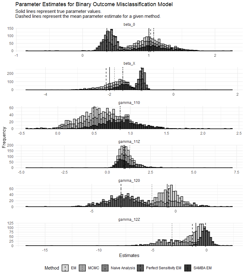
Figure 2: (Caption on next page.)

Figure 2 Caption: Parameter estimates for 500 realizations of simulation Setting 1. “EM” and “MCMC” estimates were computed using the COMBO R Package. The “SAMBA EM” results assume perfect specificity and were computed using the SAMBA R Package. The “Perfect Sensitivity EM” results were computed using an adapted function from the SAMBA R Package ⁷. The “Naive Analysis” results were obtained by running a simple logistic regression model for $Y^{*}\sim X$. Solid lines represent true parameter values. Dashed lines represent mean parameter estimates for a given method.

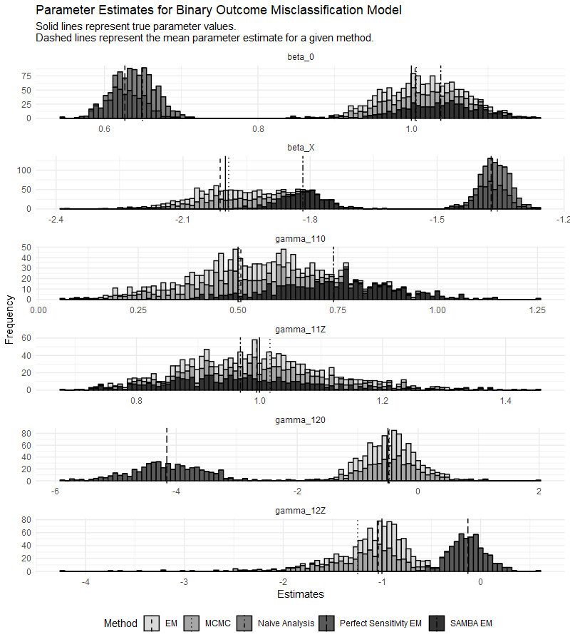
Figure 3: (Caption on next page.)

Figure 3 Caption: Parameter estimates for 500 realizations of simulation Setting 2. “EM” and “MCMC” estimates were computed using the COMBO R Package. The “SAMBA EM” results assume perfect specificity and were computed using the SAMBA R Package. The “Perfect Sensitivity EM” results were computed using an adapted function from the SAMBA R Package ⁷. The “Naive Analysis” results were obtained by running a simple logistic regression model for $Y^{*}\sim X$. Solid lines represent true parameter values. Dashed lines represent mean parameter estimates for a given method.

Simulation Setting 3 Results Figure

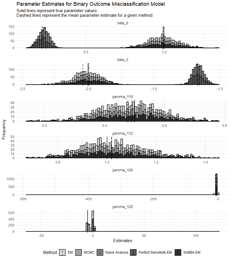
Figure 4: (Caption on next page.)

Figure 4 Caption: Parameter estimates for 500 realizations of simulation Setting 3. “EM” and “MCMC” estimates were computed using the COMBO R Package. The “SAMBA EM” results assume perfect specificity and were computed using the R Package. The “Perfect Sensitivity EM” results were computed using an adapted function from the SAMBA R Package ⁷. The “Naive Analysis” results were obtained by running a simple logistic regression model for $Y^{*}\sim X$. Solid lines represent true parameter values. Dashed lines represent mean parameter estimates for a given method.

References

- 1 Manski Charles F, Molinari Francesca. Estimating the COVID-19 infection rate: Anatomy of an inference problem Journal of Econometrics. 2021;220:181–192.
- 2 Ge Lin, Zhang Yuzi, Waller Lance A, Lyles Robert H. Enhanced Inference for Finite Population Sampling-Based Prevalence Estimation with Misclassification Errors arXiv preprint arXiv:2302.03558. 2023.
- 3 Trangucci Rob, Chen Yang, Zelner Jon. Identified vaccine efficacy for binary post-infection outcomes under misclassification without monotonicity arXiv preprint arXiv:2211.16502. 2022.
- 4 Althubaiti Alaa. Information bias in health research: definition, pitfalls, and adjustment methods Journal of Multidisciplinary Healthcare. 2016;9:211-217.
- 5 Sinnott Jennifer A, Dai Wei, Liao Katherine P, et al. Improving the power of genetic association tests with imperfect phenotype derived from electronic medical records Human Genetics. 2014;133:1369–1382.
- 6 Kahn Shihab. An introduction to classification using mislabeled data. Towards Data Science URL 2020. https://towardsdatascience.com/an-introduction-to\\-classification-using-mislabeled-data-581a6c09f9f5 [accessed 30 September 2022].
- 7 Beesley Lauren J, Mukherjee Bhramar. Statistical inference for association studies using electronic health records: handling both selection bias and outcome misclassification Biometrics. 2022;78:214–226.
- 8 Zhang Qihuang, Yi Grace Y. Genetic association studies with bivariate mixed responses subject to measurement error and misclassification Statistics in Medicine. 2020;39:3700–3719.
- 9 Neuhaus John M. Bias and efficiency loss due to misclassified responses in binary regression Biometrika. 1999;86:843–855.
- 10 Lyles Robert H, Tang Li, Superak Hillary M, et al. Validation data-based adjustments for outcome misclassification in logistic regression: an illustration Epidemiology (Cambridge, MA). 2011;22:589.
- 11 Lyles Robert H, Lin Ji. Sensitivity analysis for misclassification in logistic regression via likelihood methods and predictive value weighting Statistics in medicine. 2010;29:2297–2309.
- 12 Fogliato Riccardo, Chouldechova Alexandra, G’Sell Max. Fairness evaluation in presence of biased noisy labels in International Conference on Artificial Intelligence and Statistics:2325–2336Proceedings of Machine Learning Research 2020.
- 13 Magder Laurence S, Hughes James P. Logistic regression when the outcome is measured with uncertainty American Journal of Epidemiology. 1997;146:195–203.
- 14 Paulino Carlos D, Soares Paulo, Neuhaus John. Binomial regression with misclassification Biometrics. 2003;59:670–675.
- 15 Carroll Raymond J, Ruppert David, Stefanski Leonard A, Crainiceanu Ciprian M. Measurement Error in Nonlinear Models: A Modern Perspective. Chapman and Hall/CRC 2006.
- 16 Stamey James D, Bratcher Tom L, Young Dean M. Parameter subset selection and multiple comparisons of Poisson rate parameters with misclassification Computational Statistics & Data Analysis. 2004;45:467–479.
- 17 Xia Michelle, Gustafson Paul. Bayesian inference for unidirectional misclassification of a binary response trait Statistics in Medicine. 2018;37:933–947.
- 18 Rekaya Romdhane, Smith Shannon, Hay El Hamidi, Farhat Nourhene, Aggrey Samuel E. Analysis of binary responses with outcome-specific misclassification probability in genome-wide association studies The Application of Clinical Genetics. 2016;9:169–177.
- 19 Faraone Stephen V., Tsuang Ming T.. Measuring diagnostic accuracy in the absence of a "gold standard" American Journal of Psychiatry. 1994;151:650-657. PMID: 8166304.
- 20 O’Neill Donal. Measuring obesity in the absence of a gold standard Economics & Human Biology. 2015;17:116–128.
- 21 Smith Shannon, Hay El Hamidi, Farhat Nourhene, Rekaya Romdhane. Genome wide association studies in presence of misclassified binary responses BMC Genetics. 2013;14:1–10.
- 22 Rekaya R, Weigel KA, Gianola D. Threshold model for misclassified binary responses with applications to animal breeding Biometrics. 2001;57:1123–1129.
- 23 Ziegler Gabriel. Binary Classification Tests, Imperfect Standards, and Ambiguous Information arXiv preprint arXiv:2012.11215. 2020.
- 24 Frénay Benoît, Verleysen Michel. Classification in the presence of label noise: a survey IEEE Transactions on Neural Networks and Learning Systems. 2013;25:845–869.
- 25 Bandi Hari, Bertsimas Dimitris. The price of diversity arXiv preprint arXiv:2107.03900. 2021.
- 26 Duan Rui, Ning Yang, Shi Jiasheng, Carroll Raymond J, Cai Tianxi, Chen Yong. On the global identifiability of logistic regression models with misclassified outcomes arXiv preprint arXiv:2103.12846. 2021.
- 27 Redner Richard A, Walker Homer F. Mixture densities, maximum likelihood and the EM algorithm SIAM Review. 1984;26:195–239.
- 28 Rodríguez Carlos E, Walker Stephen G. Label switching in Bayesian mixture models: Deterministic relabeling strategies Journal of Computational and Graphical Statistics. 2014;23:25–45.
- 29 Yao Weixin. Label switching and its solutions for frequentist mixture models Journal of Statistical Computation and Simulation. 2015;85:1000–1012.
- 30 Betancourt Michael. Identifying Bayesian Mixture Models URL 2017. https://betanalpha.github.io/assets/case_studies/identifying_mixture_models.html [accessed 30 September 2022].
- 31 Stephens Matthew. Dealing with label switching in mixture models Journal of the Royal Statistical Society: Series B (Statistical Methodology). 2000;62:795–809.
- 32 Ni Jiayi, Dasgupta Kaberi, Kahn Suzan R, et al. Comparing external and internal validation methods in correcting outcome misclassification bias in logistic regression: a simulation study and application to the case of postsurgical venous thromboembolism following total hip and knee arthroplasty Pharmacoepidemiology and Drug Safety. 2019;28:217–226.
- 33 Diop Aba, Diop Aliou, Dupuy Jean-François. Maximum likelihood estimation in the logistic regression model with a cure fraction 2011.
- 34 Identifiability of finite mixtures of logistic regression models Journal of statistical planning and inference. 1991;27:375–381.
- 35 Kelley Mary E, Anderson Stewart J. Zero inflation in ordinal data: Incorporating susceptibility to response through the use of a mixture model Statistics in medicine. 2008;27:3674–3688.
- 36 Arber Sara, McKinlay John, Adams Ann, Marceau Lisa, Link Carol, O’Donnell Amy. Patient characteristics and inequalities in doctors’ diagnostic and management strategies relating to CHD: a video-simulation experiment Social Science & Medicine. 2006;62:103–115.
- 37 Maserejian Nancy N, Link Carol L, Lutfey Karen L, Marceau Lisa D, McKinlay John B. Disparities in physicians’ interpretations of heart disease symptoms by patient gender: results of a video vignette factorial experiment Journal of Women’s Health. 2009;18:1661–1667.
- 38 McKinlay John B, Potter Deborah A, Feldman Henry A. Non-medical influences on medical decision-making Social Science & Medicine. 1996;42:769–776.
- 39 Dempster Arthur P, Laird Nan M, Rubin Donald B. Maximum likelihood from incomplete data via the EM algorithm Journal of the Royal Statistical Society: Series B (Methodological). 1977;39:1–22.
- 40 Agresti Alan. Categorical Data Analysis. New York: John Wiley & Sons 2003.
- 41 AHRQ . Medical Expenditure Panel Survey. Rockport, MD: U.S. Department of Health and Human Services 2022.
- 42 Turkbey Evrim B, Nacif Marcelo S, Guo Mengye, et al. Prevalence and correlates of myocardial scar in a US cohort JAMA. 2015;314:1945–1954.
- 43 R Core Team . R: A Language and Environment for Statistical Computing. R Foundation for Statistical ComputingVienna, Austria 2021.