Calculus ++ Generalized Differential and Integral Calculus and Heisenberg’s Uncertainty Principle

Abstract

This paper presents a generalization for Differential and Integral Calculus. Just as the derivative is the instantaneous angular coefficient of the tangent line to a function, the generalized derivative is the instantaneous parameter value of a reference function (derivator function) tangent to the function. The generalized integral reverses the generalized derivative, and its calculation is presented without antiderivatives. Generalized derivatives and integrals are presented for polynomial, exponential and trigonometric derivators and integrators functions. As an example of the application of Generalized Calculus, the concept of instantaneous value provided by the derivative is used to precisely determine time and frequency (or position and momentum) in a function (signal or wave function), opposing Heisenberg’s Uncertainty Principle.

1 Introduction

Differential and Integral Calculus has become one of the main mathematical tools that made possible discoveries and advances in several areas such as Physics, Chemistry, Economics, Computer Science, Engineering, and even Biology and Medicine. Moreover, in Mathematics itself, Differential and Integral Calculus is used in other areas, such as Linear Algebra, Analytical Geometry, Probability, and Optimization, among others.

Differential and Integral Calculus was developed by Isaac Newton Newton1736 (1643-1727) and Gottfried Wilhelm Leibniz Leibniz1684 (1646-1716), independently of each other, in the 17th century and basically established three operations that are applicable to any function: calculus of limits, derivatives, and integrals.

The derivative concerns the instantaneous rate of change of a function. On the other hand, the integral concerns the area under the curve described by a function. Both the derivative and the integral are based on the calculus of infinitesimals through the concept of limit, and the Fundamental Theorem of Calculus formalizes the inverse operations relationship between Differential and Integral Calculus.

The derivative is an operation that is performed on any function $f(x)$, resulting in another function $f^{\prime}(x)$ that represents the slope of the tangent line to $f(x)$ for each x. Differential Calculus uses the line as the “reference function” and its slope as the result of the derivative.

Remark.

Why use only the line as the reference function and its slope as the result of the derivative?

This paper presents the derivative performed for other reference functions different from the line and other parameters different from the slope of the line, thus generalizing the Differential Calculus.

Since the derivative and the integral are inverse operations, the same generalization concept employed for Differential Calculus is applied to Integral Calculus.

1.1 The Derivative, its Generalization and the Antiderivative

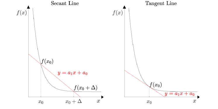
The derivative of a function can be understood as a linear interpolation process. Let $\mathbb{I}$ a non-empty open interval, $f:\mathbb{I}\to\mathbb{R}$ a function, $y=f(x)$, $\mathbb{I}\subseteq\mathbb{R}$, $x_{0}\in\mathbb{I}$ and $\Delta\in\mathbb{R}$, as illustrated in figure 1.

Two points determine a line: from the points $(x_{0},f(x_{0}))$ and $(x_{0}+\Delta,f(x_{0}+\Delta))$ it is possible to calculate the angular ($a_{1}$) and linear ($a_{0}$) coefficient of the linear equation $y=a_{1}x+a_{0}$ secant to the graph of the function $f(x)$. This calculation is obtained by solving the following linear system:

$$S:\left\{\begin{array}[]{ll}f(x_{0})=a_{1}x_{0}+a_{0}\\ f(x_{0}+\Delta)=a_{1}(x_{0}+\Delta)+a_{0}\end{array}\right.$$ (1)

The resolution of 1 is:

$$a_{1}=\frac{f(x_{0}+\Delta)-f(x_{0})}{\Delta}$$ (2)

$$a_{0}=\frac{f(x_{0})(x_{0}+\Delta)-f(x_{0}+\Delta)x_{0}}{\Delta}$$ (3)

Figure 1: Secant line (red) passing through the points $(x_{0},f(x_{0}))$ and $(x_{0}+\Delta,f(x_{0}+\Delta))$ (left figure) and the tangent line at point $(x_{0},f(x_{0}))$ (right figure) to the function (black).

In differential calculus, the angular coefficient ($a_{1}$) in (2) is known as Newton’s Difference Quotient.

For small $\Delta$ values, the linear equation $y=a_{1}x+a_{0}$ will be practically tangential to the graph of the function $f(x)$ near the point $x_{0}$, and in the limit $\Delta\to 0$, this line will be tangential to the graph of $f(x)$ at point $x_{0}$. Applying limit of $\Delta\to 0$ in (1) is:

$$S:\left\{\begin{array}[]{ll}f(x_{0})=a_{1}x_{0}+a_{0}\\ f(x_{0}+\Delta\to 0)=a_{1}(x_{0}+\Delta\to 0)+a_{0}\end{array}\right.$$ (4)

And, its resolution is:

$$a_{1}\mid_{x_{0}}=\displaystyle\lim_{\Delta\to 0}\frac{f(x_{0}+\Delta)-f(x_{0})}{\Delta}$$ (5)

$$a_{0}\mid_{x_{0}}=\displaystyle\lim_{\Delta\to 0}\frac{f(x_{0})(x_{0}+\Delta)-f(x_{0}+\Delta)x_{0}}{\Delta}$$ (6)

In (5), the value of $a_{1}\mid_{x_{0}}$ is the value of the derivative of $f(x)$ at the point $x_{0}$. The value of $a_{0}\mid_{x_{0}}$ in (6) is not used in traditional differential and integral calculus. Generalizing for any point $x$ in the domain, $a^{ins}_{1}:\mathbb{I}\to\mathbb{R}$ the function $a_{1}$ instantaneous, the derivative of $f(x)$ is:

$$\frac{df(x)}{dx}=a^{ins}_{1}(x)=\lim_{\Delta\to 0}\frac{f(x+\Delta)-f(x)}{\Delta}$$ (7)

Remark.

Therefore, the derivative of a function is the application of the limit of $\Delta\to 0$ to Newton’s Difference Quotient.

This process uses a linear procedure to determine the slope (angular coefficient) of the linear equation of the tangent line to any function at a given point. This linear procedure is simply a linear interpolation or a regression to the linear equation for two infinitesimally close points belonging to $f(x)$. However, similarly to (7), from (6), $a^{ins}_{0}:\mathbb{I}\to\mathbb{R}$ the function $a_{0}$ instantaneous, one can write:

$$\begin{array}[]{ll}\displaystyle\mathfrak{D}\{\}=a_{1}x+a_{0}\\ \displaystyle\mathfrak{D}\{a_{0}\}\frac{df(x)}{dx}=a^{ins}_{0}(x)=\lim_{\Delta\to 0}\frac{f(x)(x+\Delta)-f(x+\Delta)x}{\Delta}\end{array}$$ (8)

where,

$\mathfrak{D}\{\}$ is the tangent function to $f(x)$ in which the derivative is defined (the line equation in this case, as in the “classical derivative”, but it could be any other function);

$\mathfrak{D}\{a_{0}\}\frac{df(x)}{dx}$ indicates under which parameter of the $\mathfrak{D}\{\}$ the derivative $\frac{df(x)}{dx}$ is defined.

In this context, as (8), the generalized notation for the “classical derivative” (7) is:

$$\begin{array}[]{ll}\displaystyle\mathfrak{D}\{\}=a_{1}x+a_{0}\\ \displaystyle\mathfrak{D}\{a_{1}\}\frac{df(x)}{dx}=a^{ins}_{1}(x)=\lim_{\Delta\to 0}\frac{f(x+\Delta)-f(x)}{\Delta}\end{array}$$ (9)

The reasoning used in (1) to (9) can be generalized to other functions (and not just the linear equation) and their respective parameters. This concept can also be applied to the integral of a function. For example, the notation for the inverse operation of (9) is:

$$\begin{array}[]{ll}\displaystyle\mathfrak{I}\{\}=a_{1}x+a_{0}\\ \displaystyle F(x)=\mathfrak{I}\{a_{1}\}\int f(x)dx\end{array}$$ (10)

where,

$\mathfrak{I}\{\}$ is the tangent function to $F:\mathbb{I}\to\mathbb{R}$ which the integral is defined;

$\mathfrak{I}\{a_{1}\}\int f(x)dx$ indicates under which parameter of the $\mathfrak{I}\{\}$ the integral of $f(x)$ is defined.

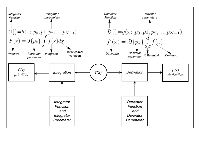
As a result, the following concepts can be defined:

• Derivator Function is the function $\mathfrak{D}\{\}$ that is used in the interpolation process (the classic derivative uses the linear equation as Derivator Function).

• Derivator Parameter is the parameter of interest $p_{k}$ of the $\mathfrak{D}\{\}$, represented by $\mathfrak{D}\{p_{k}\}$, where $p_{k}\in\mathfrak{P}$, $\mathfrak{P}=\{p_{0},p_{1},p_{2},...,p_{N-1}\}$ is the set of $N\in\mathbb{N}$ parameters of the $\mathfrak{D}\{\}$, $k\in\mathbb{N}$ and $k<N$ . (the classic derivative uses the angular coefficient $a_{1}$ as Derivator Parameter).

• Integrator Function is the function $\mathfrak{I}\{\}$ that is used in the process of obtaining the primitive function (the classic integral uses the linear equation as Integrator Function).

• Integrator Parameter is the parameter of interest $p_{k}$ of the $\mathfrak{I}\{\}$, represented by $\mathfrak{I}\{p_{k}\}$, where $p_{k}\in\mathfrak{Q}$, $\mathfrak{Q}=\{p_{0},p_{1},p_{2},...,p_{N-1}\}$ is the set of $N\in\mathbb{N}$ parameters of the $\mathfrak{I}\{\}$, $k\in\mathbb{N}$ and $k<N$ . (the classic integral uses the angular coefficient $a_{1}$ as Integrator Parameter).

Figure 2 illustrates the names of the functions and operations involved in Generalized Differential and Integral Calculus.

Figure 2: Functions and operations involved in Differential and Integral Calculus.

2 Background

Different forms of the derivative have already been established. These forms use concepts different from the foundation employed for generalizing Differential and Integral Calculus presented in this article.

• Symmetric Derivative Aull1967

A simple variant form of the “classical derivative” is the Symmetric Derivative, which uses Newton’s Difference Quotient in a symmetrical form. The Symmetric Derivative $f^{\prime}_{S}$ is defined as:

$$f^{\prime}_{S}=\lim_{\Delta\to 0}\frac{f(x+\Delta)-f(x-\Delta)}{2\Delta}$$ (11)

Although the Symmetric Derivative uses a different form for Newton’s Difference Quotient, the derivative function can still be understood as the slope of the tangent line to the function $f(x),\forall{x}$. In this form, the Symmetric Derivative is a different manner of defining the “classical derivative”.

• Fréchet Derivative Coleman2012

Given $\mathbb{V}$ and $\mathbb{U}$ normed vectorial spaces, $\mathbb{W}\subseteq\mathbb{V}$, $f:\mathbb{W}\to\mathbb{U}$ a function Fréchet differentiable at $x\in\mathbb{V}$. If there is a bounded and linear operator $A:\mathbb{V}\to\mathbb{U}$ such that:

$$\lim_{\Delta\to 0}\frac{\parallel f(x+\Delta)-f(x)-A\Delta\parallel_{\mathbb{U}}}{\parallel\Delta\parallel_{\mathbb{V}}}=0$$ (12)

Then, $A$ is the derivative of $f$ at $x$. The Fréchet Derivative is used on a vector-valued function of multiple real variables and to define the Functional Derivative, generalizing the derivative of a real-valued function of a single real variable.

• Functional Derivative Coleman2012

Another form of a derivative is the Functional Derivative. Given $\mathbb{V}$ a vectorial (function) space, $\mathbb{K}$ a field and $F$ a functional, $F:\mathbb{V}\to\mathbb{K}$, $f\in\mathbb{V}$, $\zeta$ an arbitrary function, the Functional Derivative of $F$ at $f$, $\frac{d(F)}{d(f)}$ is:

$$\int{}{}{\frac{d(F)}{d(f)}}(x)\zeta(x)dx=\lim_{\Delta\to 0}\frac{F(f+\Delta\zeta)-F(f)}{\Delta}$$ (13)

In this case, the concept of the derivative is applied to a functional and not to a function. In this paper, the concept of the derivative is generalized to functions.

• Fractional Derivative Golmankhaneh2022

The derivative can be repeated $n$ times over a function, resulting in the derivative’s order. Thus, the order of the derivative is clearly a natural number ($n\in\mathbb{N})$. The fractional derivative generalizes the concept of derivative order so that the $\alpha$ order of the fractional derivative is $\alpha\in\mathbb{R}$ or even $\alpha\in\mathbb{C}$. It is then possible, under this generalization, to calculate the derivative of $f(x)$ of order $alpha=2.5$ or $alpha=-1$ (integral of $f(x)$), for example. In this paper, the derivative is generalized to functions and not to the order of the derivative.

• q-Derivative Chaundy1962

The q-Derivative of a function $f(x)$ is a q-analog of the “classic derivative”. Let $q\in\mathbb{R}$, it is given by:

$${\left(\frac{d}{dx}\right)_{q}f(x)}=\frac{f(qx)-f(x)}{qx-x}$$ (14)

For $q\to 1$, the q-Derivative is the “classic derivative”.

• Arithmetic Derivative Haukkanen2018

Let $a.b\in\mathbb{N}$ and $p$ a prime number, the arithmetic derivative $D(a.b)$ is such that:

$$\begin{array}[]{ll}D(0)=D(1)=0\\ D(p)=1,\forall\mbox{ prime }p\\ D(a.b)=D(a)b+a.D(b)\end{array}$$ (15)

The Arithmetic Derivative is a ”number derivative”, which is based on prime factorization. The arithmetic derivative can be extended to rational numbers.

Other forms of derivatives include:

• Carlitz derivative Kochubei2007

• Covariant derivative Zuk1986

• Dini derivative Kannan1996

• Exterior derivative Tu2007

• Gateaux derivative Andrews2011

• H derivative Kac2002

• Hasse derivative Hoffmann2015

• Lie derivative Lee2003

• Pincherle derivative Mainardi2011

• Quaternionic derivative Xu2015

• Radon Nikodym derivative Konstantopoulos2011

• Semi differentiability Luc2018

• Subderivative Rockafellar1998

• Weak derivative Lamboni2022

All of these forms use concepts different from the foundation employed for the generalization of Differential and Integral Calculus presented in this article.

3 Polynomials Derivators Functions

Let $n\in\mathbb{N}$, $a_{i}\in\mathbb{R}$, $\forall{i}\in\mathbb{N}$, $P:\mathbb{R}\to\mathbb{R}$ is a Polynomial Function if:

$$P(x)=a_{n}x^{n}+a_{n-1}x^{(n-1)}+....+a_{1}x^{1}+a_{0}x^{0}=\sum_{i=0}^{n}a_{i}x^{i}$$ (16)

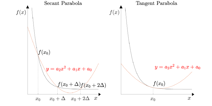
In (16), the value of $n$ defines the degree of the polynomial. For $n=1$, the polynomial is a linear equation, and two points are needed to define its parameters (as in (1)). For $n=2$ and $n=3$, the polynomial is a quadratic (parabola) and cubic function, and 3 and 4 points are needed to define their parameters, respectively. For other degrees of the polynomial, the reasoning is analogous; therefore, $n+1$ points are necessary to define the parameters of a polynomial of degree n. Using a polynomial of degree 2 ($n=2$) as derivator function, the derivative becomes an interpolation process to the quadratic function for three infinitesimally close points belonging to $f(x)$, resulting in the Parabolic Derivative, as shown in figure 3.

Figure 3: Secant parabola (red) passing through the points $x_{0}$, $x_{0}+\Delta$ and $x_{0}+2\Delta.$ (left figure) and tangent parabola at point $x_{0}$ (right figure) to the function (black).

The system is:

$$S:\left\{\begin{array}[]{ll}f(x_{0})=a_{2}x_{0}^{2}+a_{1}x_{0}+a_{0}\\ f(x_{0}+\Delta)=a_{2}(x_{0}+\Delta)^{2}+a_{1}(x_{0}+\Delta)+a_{0}\\ f(x_{0}+2\Delta)=a_{2}(x_{0}+2\Delta)^{2}+a_{1}(x_{0}+2\Delta)+a_{0}\end{array}\right.$$ (17)

Generalizing for any point $x$ in the domain, $a^{ins}_{0}:\mathbb{I}\to\mathbb{R}$ the function $a_{0}$ instantaneous, $a^{ins}_{1}:\mathbb{I}\to\mathbb{R}$ the function $a_{1}$ instantaneous, $a^{ins}_{2}:\mathbb{I}\to\mathbb{R}$ the function $a_{2}$ instantaneous, and applying limit to $\Delta\to 0$, the resolution of (17) is:

$$\mathfrak{D}\{\}=a_{2}x^{2}+a_{1}x+a_{0}$$ (18)

$$\mathfrak{D}\{a_{2}\}\frac{df(x)}{dx}=a^{ins}_{2}(x)=\lim_{\Delta\to 0}\frac{1}{2}\frac{f(x)-2f(x+\Delta)+f(x+2\Delta)}{\Delta^{2}}$$ (19)

$$\mathfrak{D}\{a_{1}\}\frac{df(x)}{dx}=a^{ins}_{1}(x)=\lim_{\Delta\to 0}-\frac{1}{2}\frac{K_{0}f(x)-K_{1}f(x+\Delta)+K_{2}f(x+2\Delta)}{\Delta^{2}}\\$$ (20)

where,

$$K_{0} =2x+3\Delta$$

$$K_{1} =4x+4\Delta$$

$$K_{2} =2x+\Delta$$

$$\mathfrak{D}\{a_{0}\}\frac{df(x)}{dx}=a^{ins}_{0}(x)=\lim_{\Delta\to 0}\frac{1}{2}\frac{K_{0}f(x)+K_{1}f(x+\Delta)+K_{2}f(x+2\Delta)}{\Delta^{2}}\\$$ (21)

where,

$$K_{0} =2\Delta^{2}+x^{2}+3x\Delta$$

$$K_{1} =-2x^{2}-4x\Delta$$

$$K_{2} =x^{2}+x\Delta$$

In this form, (19), (20) and (21) define the Parabolic Derivative to the $a_{2}$, $a_{1}$ and $a_{0}$ parameters, respectively. For polynomials of other degrees, the procedure is similar to that performed in (17). For example, the generalized polynomial derivative (polynomial derivator function) of $f(x)=cx^{m}$, $c,m\in\mathbb{R}$ for the highest degree parameter $n\in\mathbb{N^{*}}$ of the polynomial derivator function is:

$$\mathfrak{D}\{\}={a_{n}}x^{n}+a_{n-1}x^{(n-1)}+...+a_{1}x^{1}+a_{0}x^{0}$$ (22)

$$\mathfrak{D}\{{a_{n}}\}\frac{d(cx^{m})}{dx}=c\left(\prod_{i=0}^{n-1}\frac{m-i}{i+1}\right)x^{(m-n)}=\;$$

$$\frac{c}{n!}\left(\prod_{i=0}^{n-1}{(m-i)}\right)x^{(m-n)}\;\;\;\;\;$$ (23)

The Antiderivative of (3) is:

$$\mathfrak{I}\{\}=\mathfrak{D}\{\}={a_{n}}x^{n}+a_{n-1}x^{(n-1)}+...+a_{1}x^{1}+a_{0}x^{0}$$ (24)

$$\begin{array}[]{ll}\mathfrak{I}\{{a_{n}}\}\int{cx^{m}}{dx}=\left(\frac{cx^{(m+n)}}{(m+n)\prod_{i=1}^{n-1}{\frac{m+i}{i+1}}}\right),\forall{(m+n)\neq{0}\wedge n\geq 2}\\ \mathfrak{I}\{{a_{1}}\}\int{cx^{m}}{dx}=\left(\frac{cx^{(m+1)}}{(m+1)}\right),m\neq{-1}\end{array}$$ (25)

For the other functions $f(x)$ and/or other derivator parameters, the reasoning is analogous to (17), (3) and (25).

3.1 Vanishing Terms and Primitives

The “classic derivative” uses the linear equation as the derivator function and the angular coefficient as the derivator parameter (as in (9)). However the derivative in this form does not model the linear coefficient of the derivator function, and therefore this term, if it exists in the derivand $f(x)$, “vanishes” for the differential operator, not influencing the derivative. Using the linear equation as the derivator function and the linear coefficient as the derivator parameter as in (8), the derivative in this form does not model the first-degree term (angular coefficient) of the derivator function. Therefore, this term ”vanishes” for the differential operator, not influencing the derivative. The following example is suitable for showing this case. Considering:

$$f(x)=x^{2}+2x+3$$ (26)

for $\mathfrak{D}\{\}=a_{1}x+a_{0}$, their derivatives are:

$$\mathfrak{D}\{a_{1}\}\frac{df(x)}{dx}=2x+2$$ (27)

and

$$\mathfrak{D}\{a_{0}\}\frac{df(x)}{dx}=-x^{2}+3$$ (28)

The term $+3$ and $2x$ in (26) vanishes in (27) and (28), respectively. For $\mathfrak{I}\{\}=a_{1}x+a_{0}$, the antiderivatives, respectively, for (27) and (28) are:

$$\mathfrak{I}\{a_{1}\}\int(2x+2)dx=x^{2}+2x$$ (29)

and

$$\mathfrak{I}\{a_{0}\}\int(-x^{2}+3)dx=x^{2}+3$$ (30)

Since (27) and (28) do not model the terms $a_{0}$ and $a_{1}x$, respectively, the antiderivatives (29) and (30) do not return in (26) and must be added by the following terms ($k_{0}$ and $k_{1}x$, with $k_{0}$ and $k_{1}$ constants):

$$\mathfrak{I}\{a_{1}\}\int(2x+2)dx=x^{2}+2x+k_{0}$$ (31)

and

$$\mathfrak{I}\{a_{0}\}\int(-x^{2}+3)dx=x^{2}+k_{1}x+3$$ (32)

The addition of the terms $k_{0}$ and $k_{1}x$ in (31) and (32) is necessary because, independently of $k_{0}$ and $k_{1}x$, their derivatives are the same:

$$\mathfrak{D}\{a_{1}\}\frac{d(x^{2}+2x+k_{0})}{dx}=2x+2$$ (33)

and

$$\mathfrak{D}\{a_{0}\}\frac{d(x^{2}+k_{1}x+3)}{dx}=-x^{2}+3$$ (34)

3.2 Integrals without Antiderivatives

The Fundamental Theorem of Calculus (FTC) Strang1991 establishes the relationship between differential calculus and integral calculus, as inverse operations (with reservations). The FTC is divided into two parts. Part 1 shows that the derivative of the integral of $f(x)$ is equal to $f(x)$: this is perfect! Part 2 reverses the order, that is, the integral of the derivative of $f(x)$ is equal to $f(x)$, however, plus a constant $k$, that is, $f(x)+k$: this is perfect too, but the exact return to function $f(x)$ does not occur when the derivative is performed first and then the integral. Thus, in formal terms, the FTC states that the operations of derivation and integration are inverse, apart from a constant value.

$$\frac{d\int f(x)dx}{dx}=f(x)\neq\int\frac{df(x)}{dx}dx=f(x)+k$$ (35)

This problem occurs simply because the “classic derivative” only gives the instantaneous rate of change of a function for its domain. This rate, as seen in (5), is the angular coefficient for the linear equation when used as derivator function. Obviously, the linear equation cannot be defined by its angular coefficient $a_{1}$ alone. The linear coefficient $a_{0}$ also needs to be defined for the linear equation to be complete.

The derivation process is carried out by applying the concept of limit to Newton’s quotient. On the other hand, the integration process does not have a specific form, and this is obtained, in practice, through the calculation of antiderivatives. Nonetheless, a function can be defined by applying the integrator function $\mathfrak{I}\{\}$ to the generalized derivatives for a given derivator function $\mathfrak{D}\{\}$ for all their respective parameters, with $\mathfrak{I}\{\}=\mathfrak{D}\{\}$.

For the integrator function $\mathfrak{I}\{\}:a_{1}x+a_{0}$ (linear equation) and $\mathfrak{I}\{\}=\mathfrak{D}\{\}$, the primitive $f(x)$ is:

$$f(x)=\mathfrak{D}\{a_{1}\}\frac{df(x)}{dx}x+\mathfrak{D}\{a_{0}\}\frac{df(x)}{dx}$$ (36)

It is important to emphasize that $f(x)$ was obtained from its generalized derivatives without the conventionally used integration process (antiderivative) in “classical integral calculus”.

For example, from the functions (27) and (28) (derivatives of $f(x)=x^{2}+2x+3$), the primitive $f(x)$ is:

$$f(x)=(2x+2)x-x^{2}+3=x^{2}+2x+3$$ (37)

The exact return to $f(x)$ is obtained ((37) equals (26)). The concept involved in obtaining the function $f(x)$ is:

Theorem.

Let $\mathbb{I}$ a non-empty open interval, $\mathbb{I}\subseteq\mathbb{C}$, $h:\mathbb{I}\to\mathbb{C}$ a function, $y=h(x\mathchar 24635\relax\;p_{0},p1,p_{2},...,p_{N-1})$ and $\mathfrak{P}=\{p_{0},p_{1},p_{2},...,p_{N-1}\}$ the set of $N\in\mathbb{N}$ parameters. If S is a system that has a unique solution for $N$ points $(x_{k},y_{k})$, $k\in\mathbb{N}$, $k\leq{N-1}$, such as:

$$S:\left\{\begin{array}[]{ll}y_{0}=h(x_{0}\mathchar 24635\relax\;p_{0},p1,p_{2},...,p_{N-1})\\ y_{1}=h(x_{1}\mathchar 24635\relax\;p_{0},p1,p_{2},...,p_{N-1})\\ y_{2}=h(x_{2}\mathchar 24635\relax\;p_{0},p1,p_{2},...,p_{N-1})\\ ...\\ y_{N-1}=h(x_{N-1}\mathchar 24635\relax\;p_{0},p1,p_{2},...,p_{N-1})\\ \end{array}\right.$$ (38)

$\mathfrak{I}\{\}=\mathfrak{D}\{\}=h(x\mathchar 24635\relax\;p_{0},p1,p_{2},...,p_{N-1})$, $f(x)$ differentiable on $\mathfrak{D}\{\}$, $\forall{x}\in\mathbb{I}$, then f(x) can be described by $\mathfrak{I}\{\}$ whose parameters are given by their generalized derivatives in their respective $N$ parameters, i.e. $f(x)=h(x\mathchar 24635\relax\;\mathfrak{D}\{p_{0}\},\mathfrak{D}\{p_{1}\},\mathfrak{D}\{p_{2}\},...,\mathfrak{D}\{p_{N-1}\})$.

4 Exponential Derivators Functions

Let $A,a,b,x\in\mathbb{R}$, $a^{ins}:\mathbb{R}\to\mathbb{C}$, $b^{ins}:\mathbb{R}\to\mathbb{C}$ and $f:\mathbb{R}\to\mathbb{R}$ an exponential function as:

$$f(x)=Ae^{ax},A\geq 0$$ (39)

Making $A=e^{b}$, (39) is:

$$f(x)=e^{b}e^{ax}=e^{ax+b}$$ (40)

The following system can be written:

$$S:\left\{\begin{array}[]{ll}f(x)=e^{ax+b}\\ f(x+\Delta)=e^{a(x+\Delta)+b}\end{array}\right.$$ (41)

Solving the system and applying the limit of $\Delta\to 0$ in (41), the Exponential Derivative (derivator function is exponential) of a function $f(x)$ becomes:

$$\mathfrak{D}\{\}=e^{ax+b}$$ (42)

$$\mathfrak{D}\{a\}\frac{df(x)}{dx}=a^{ins}(x)=\lim_{\Delta\to 0}\frac{ln(f(x+\Delta))-ln(f(x))}{\Delta}$$ (43)

$$\mathfrak{D}\{b\}\frac{df(x)}{dx}=b^{ins}(x)=\lim_{\Delta\to 0}\frac{ln(f(x))(x+\Delta)-ln(f(x+\Delta))x}{\Delta}$$ (44)

$f(x)$ can be reconstructed from its exponential derivatives as:

$$f(x)=e^{\mathfrak{D}\{a\}\frac{df(x)}{dx}x+\mathfrak{D}\{b\}\frac{df(x)}{dx}}$$ (45)

The function $e^{-i\omega x}$ (kernel of the Fourier Transform) is discussed in the section 6.2.

5 Trigonometric Derivators Functions

Let $\omega$, $\phi$ $\in\mathbb{R}$, the frequency and phase, respectively, and $\omega^{ins}:\mathbb{R}\to\mathbb{C}$, $\phi^{ins}:\mathbb{R}\to\mathbb{C}$ the instantaneous frequency and phase, respectively, the following system can be written:

$$S:\left\{\begin{array}[]{ll}f(x)=\sin(\omega x+\phi)\\ f(x+\Delta)=\sin(\omega(x+\Delta)+\phi)\end{array}\right.$$ (46)

Solving the system and applying the limit of $\Delta\to 0$ in (46), the sinusoidal derivative (derivator function is sinusoidal) of a function $f(x)$ becomes:

$$\mathfrak{D}\{\}=\sin({\omega x+\phi)}$$ (47)

$$\begin{split}\mathfrak{D}\{\omega\}\frac{df(x)}{dx}=\omega^{ins}(x)=\lim_{\Delta\to 0}\frac{\arcsin(f(x+\Delta))-\arcsin(f(x))}{\Delta}=\\ =\lim_{\Delta\to 0}\frac{\arcsin(f(x+\Delta)\sqrt{1-f(x)^{2}}-f(x)\sqrt{1-f(x+\Delta)^{2}})}{\Delta}\end{split}$$ (48)

$$\mathfrak{D}\{\phi\}\frac{df(x)}{dx}=\phi^{ins}(x)=\lim_{\Delta\to 0}\frac{\arcsin(f(x))(x+\Delta)-\arcsin(f(x+\Delta))x}{\Delta}$$ (49)

The same can be written to cosine and tangent functions:

$$\mathfrak{D}\{\}=\cos({\omega x+\phi)}$$ (50)

$$\begin{split}\mathfrak{D}\{\omega\}\frac{df(x)}{dx}=\omega^{ins}(x)=\lim_{\Delta\to 0}\frac{\arccos(f(x+\Delta))-\arccos(f(x))}{\Delta}=\\ =\lim_{\Delta\to 0}\frac{\arccos(f(x+\Delta)f(x)+\sqrt{(1-f(x+\Delta)^{2})(1-f(x)^{2})})}{\Delta}\end{split}$$ (51)

$$\mathfrak{D}\{\phi\}\frac{df(x)}{dx}=\phi^{ins}(x)=\lim_{\Delta\to 0}\frac{\arccos(f(x))(x+\Delta)-\arccos(f(x+\Delta))x}{\Delta}$$ (52)

$$\mathfrak{D}\{\}=\tan({\omega x+\phi)}$$ (53)

$$\begin{split}\mathfrak{D}\{\omega\}\frac{df(x)}{dx}=\omega^{ins}(x)&=\lim_{\Delta\to 0}\frac{\arctan(f(x+\Delta))-\arctan(f(x))}{\Delta}=\\ &=\frac{\arctan(\frac{f(x+\Delta)-f(x)}{1+f(x+\Delta)f(x)})}{\Delta}\end{split}$$ (54)

$$\mathfrak{D}\{\phi\}\frac{df(x)}{dx}=\phi^{ins}(x)=\lim_{\Delta\to 0}\frac{\arctan(f(x))(x+\Delta)-\arctan(f(x+\Delta))x}{\Delta}$$ (55)

If $f(x)\in[-1,1]$, (48) to (52) $\in\mathbb{R}$, otherwise (48) to (52) $\in\mathbb{C}$.

$f(x)$ can be reconstructed from its sinusoidal, cosinusoidal and tangential derivatives, respectively, as:

$$f(x)=\sin{\biggl{(}\mathfrak{D}\{\omega\}\frac{df(x)}{dx}x+\mathfrak{D}\{\phi\}\frac{df(x)}{dx}\biggr{)}}$$ (56)

$$f(x)=\cos{\biggl{(}\mathfrak{D}\{\omega\}\frac{df(x)}{dx}x+\mathfrak{D}\{\phi\}\frac{df(x)}{dx}\biggr{)}}$$ (57)

$$f(x)=\tan{\biggl{(}\mathfrak{D}\{\omega\}\frac{df(x)}{dx}x+\mathfrak{D}\{\phi\}\frac{df(x)}{dx}\biggr{)}}$$ (58)

6 Instantaneous Frequency and Heisenberg’s Uncertainty Principle

Let a phase function Jiang2020 $\Omega(x):\mathbb{R}\to\mathbb{R}$, and a waveform (signal, Wave Function Born1969 ) $\varphi(x,\omega)$ given by:

$$\varphi(x,\omega)=\sin(\Omega(x))$$ (59)

If $\Omega(x)$ is known, the determination of the instantaneous frequency $\omega(x)$ presents no difficulty and is determined by:

$$\omega(x)=\frac{d\Omega(x)}{dx}$$ (60)

However, in many real applications, $\Omega(x)$ is not known, but only the waveform $\varphi(x,\omega)$ and then, determining $\omega(x)$ or $x(\omega)$ precisely, from $\varphi(x,\omega)$ is not a possible task, according to Heisenberg’s Uncertainty Principle Heisenberg1927 , Folland1997 .

Heisenberg’s Uncertainty Principle was first proposed for Quantum Mechanics Ford2005 . However, it is used to demonstrate that there is a limit to the accuracy with which the pair of canonically conjugate variables Hjalmars1962 in phase space, ($x,\omega$) or ($x,p$), where $p$ is the momentum, e.g., can be measured simultaneously.

“…Thus, the more precisely the position is determined, the less precisely the momentum is known, and conversely…”

Heisenberg, 1927

De Broglie’s LouisVictorPierreRaymond1924 relation establishes the undulatory nature of the particle (matter) by:

$$k=\frac{p}{\hslash}$$ (61)

where, $k$ is the wavenumber (spatial frequency), $p$ is the momentum and $\hslash$ is the reduced Planck’s constant.

Thus, one can understand that determining the momentum $p$ as a function of position $x$ is equivalent to determining the wavenumber $k$ as a function of position $x$ or even the (temporal) frequency $\omega$ as a function of time $x$ ($x$, in this case, is the “position” in time) - Instantaneous Frequency.

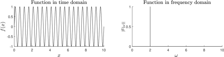
The classical mathematical operation that changes the domain of a function from time to frequency (and vice versa) is the Fourier Transform, but a non-zero function $f(x):\mathbb{R}\to\mathbb{R}$ and its Fourier Transform $F(\omega):\mathbb{R}\to\mathbb{C}$ cannot both be sharply localized Folland1997 .

The figure 4 shows a function $f(x):\mathbb{R}\to\mathbb{R}$ (a sinusoidal wave with frequency equal 2 Hz) and $\lvert F(\omega)\rvert:\mathbb{R}\to\mathbb{R}$ in $x$ (time) and $\omega$ (frequency) domain. $F(\omega)$ has no information about $x$ and $f(x)$ has no information about $\omega$.

Figure 4: Function in time and frequency domain

A Window Function $g(x):\mathbb{R}\to\mathbb{R}$ that is “well localized” in the time is used to localize the frequency in time. Figure 5 shows the wide (above) and narrow (below) window function and its respective Fourier Transform Magnitude $\lvert G(\omega)\rvert:\mathbb{R}\to\mathbb{R}$ (narrow (above) and wide (below)).

Figure 5: Window Functions in time and frequency domain.

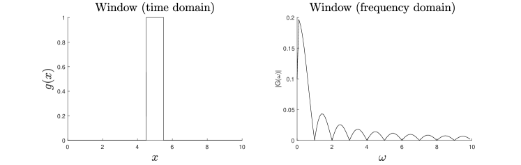
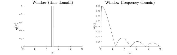
The function $f(x)$ is multiplied by the Window Function $g(x)$. Figure 6 shows the wide (above) and narrow (below) Windowed Function and its respective Fourier Transform Magnitude $\lvert F(\omega)*G(\omega)\rvert$ (narrow (above) and wide (below)).

Figure 6: Windowed Functions in time and frequency domain.

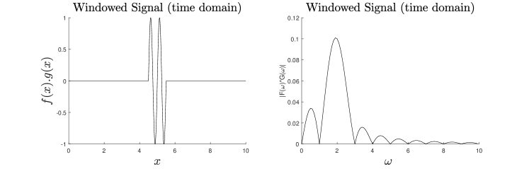
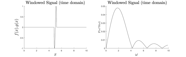
The Windowed Function in the frequency domain should have only one component (at 2 Hz), but it has components at several frequencies with non-zero amplitudes. This fact is due to the Windowed Function in the frequency domain being the result of the convolution of the function by the Window Function in the frequency domain (in an analogous form, one can use the concept of wave packets in order to locate a wave in space Rozenman2019 ). So it is impossible to identify whether a particular frequency component is due to the function or the Window Function.

To measure the frequency as a function of the time, it was necessary to “locate” the wave in time using the Window function. However, this fact goes beyond the classical concept in physics of the observer effect Schlosshauer2005 , Giacosa2014 , in which to make a measurement, it is necessary to interfere with the measurement (which causes uncertainty). As everything that exists is a wave (wave nature of matter), Heisenberg’s Uncertainty Principle states that uncertainty occurs not only due to the measurement of an experiment (observer effect) but due to the impossibility of locating a wave sharply in the time and frequency (wavenumber, momentum, among others) domain simultaneously.

Analytically, Heisenberg’s Uncertainty Principle can be demonstrated considering $\psi(x)$ and $\Psi(p)$ wave functions and Fourier Transform of each other for position $x$ and momentum $p$ , respectively.

Born’s rule Born1926 states that $\lvert\psi(x)\rvert^{2}$ and $\lvert\Psi(p)\rvert^{2}$ are probability density functions and then the variances of position $\sigma_{x}^{2}$ and momentum $\sigma_{p}^{2}$ are:

$$\sigma_{x}^{2}=\int_{-\infty}^{\infty}{x^{2}}\lvert\psi(x)\rvert^{2}\,dx\ =\int_{-\infty}^{\infty}{(x\psi(x))^{*}x\psi(x)}\,dx\$$ (62)

$$\sigma_{p}^{2}=\int_{-\infty}^{\infty}{p^{2}}\lvert\Psi(p)\rvert^{2}\,dp\ =\int_{-\infty}^{\infty}{(p\Psi(p))^{*}p\Psi(p)}\,dp\$$ (63)

Let $f(x)=x\psi(x)$:

$$\sigma_{x}^{2}=\int_{-\infty}^{\infty}{f^{*}(x)f(x)}\,dx\ =\int_{-\infty}^{\infty}{\lvert f(x)\rvert^{2}}\,dx\ =\langle f\lvert f\rangle$$ (64)

Let $\mathcal{F}\left\{.\right\}$ the Fourier transform, $-i{\hslash}\frac{d\psi(x)}{dx}$ the momentum operator in position space, $G(p)=p\Psi(p)$, $g(x)=\mathcal{F}\left\{G(p)\right\}$ and applying the Parseval’s theorem Stone2021 :

$$\sigma_{p}^{2}=\int_{-\infty}^{\infty}{G^{*}(p)G(p)}\,dp\ =\int_{-\infty}^{\infty}{\lvert G(p)\rvert^{2}}\,dp\ =\int_{-\infty}^{\infty}{\lvert g(x)\rvert^{2}}\,dx\ =\langle g\lvert g\rangle$$ (65)

Using the Cauchy–Schwarz inequality Zhou2021 :

$$\langle f\lvert f\rangle\langle g\lvert g\rangle\geq\lvert\langle f\lvert g\rangle\rvert^{2}$$ (66)

$$\lvert\langle f\lvert g\rangle\rvert^{2}\geq\operatorname{Im}(\lvert\langle f\lvert g\rangle\rvert^{2})=\biggl{(}\frac{\langle f\lvert g\rangle-\langle g\lvert f\rangle}{2i}\biggr{)}^{2}$$ (67)

$$\begin{split}\langle f\lvert g\rangle&-\langle g\lvert f\rangle=\\ =\int_{-\infty}^{\infty}{x\psi^{*}(x)\biggl{(}-i{\hslash}\frac{d\psi(x)}{dx}\biggr{)}}\,dx\ &-\int_{-\infty}^{\infty}{\biggl{(}-i{\hslash}\frac{d\psi^{*}(x)}{dx}\biggr{)}x\psi(x)}\,dx\ =i{\hslash}\end{split}$$ (68)

Applying 68 in 67:

$$\lvert\langle f\lvert g\rangle\rvert^{2}=\biggl{(}\frac{i{\hslash}}{2i}\biggr{)}^{2}=\frac{{\hslash^{2}}}{4}$$ (69)

Applying 64, 65 and 69 in 66:

$$\sigma_{x}^{2}\sigma_{p}^{2}\geq\frac{{\hslash^{2}}}{4}=\sigma_{x}\sigma_{p}\geq\frac{{\hslash}}{2}$$ (70)

The demonstration of the uncertainty principle is strictly mathematical. Any pair of variables conjugated will produce the same results as this demonstration.

Following Kennard’s consideration Choe2020 , $\Delta x=\sigma_{x}$ the uncertainty in position $x$ (proportional to the width of the Window Function in time or space domain), $\Delta p=\sigma_{p}$ the uncertainty in momentum, $h$ the Plank’s constant, Heisenberg’s Uncertainty Principle is normally presented as:

$$\Delta x\Delta p\geq\frac{h}{4\pi}$$ (71)

In the frequency domain, let $\Delta k$ be the uncertainty in wavenumber (spatial frequency) or $\Delta\omega$ the uncertainty in (temporal) frequency ($\Delta k$ or $\Delta\omega$ are proportional to the width of the Window Function in frequency domain). Through de Broglie´s relation 61, 71 can be written as:

$$\Delta x\Delta k\geq\frac{1}{2\pi}\>\>\>\>\textrm{or}\>\>\>\>\Delta x\Delta\omega\geq\frac{1}{2\pi}$$ (72)

Another way to understand Heisenberg’s Uncertainty Principle (and perhaps the simplest) is through the Fourier Transform of the Gaussian function. Let $f(x)$ be a Gaussian function in the space (time) domain $x$, $F(\omega)$ is its Fourier transform in the frequency domain $\omega$ and is also a Gaussian function. Then, the standard deviation $\sigma$ can be understood as a measure of precision, and this occurs inversely in $f(x)$ and $F(\omega)$. Thus, if the uncertainty is small in one domain, it is large in the other domain.

$$f(x)=e^{-\sigma x^{2}}\Leftrightarrow F(\omega)=\frac{1}{\sqrt{2\sigma}}e^{-\frac{\omega^{2}}{4\sigma}}$$ (73)

A time-frequency representation is used when it is necessary to “localize” $\omega$ in $x$ (instantaneous frequency) and vice-versa. This representation is also known as a spectrogram, generally obtained through the Short Time Fourier Transform Groechenig2001 (or other transforms, such as Wavelet Transform Strang1996 , Wigner-Ville distribution function Hlawatsch1997 , etc).

A classic example of a signal whose frequency varies with time (non-stationary signal) is the Chirp Signal Gretinger2014 .

6.1 Chirp Derivative

A Chirp Signal can be defined with the following waveform (signal):

$$f(x)=\sin(2\pi\int{\omega(x)}dx+\phi),$$ (74)

where, $\omega(x)$ is the instantaneous frequency function and $\Omega(x)=2\pi\int{\omega(x)}dx+\phi$ is the phase function.

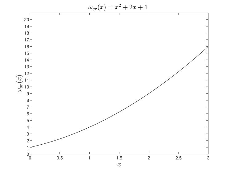
The following example is suitable for showing the determination of the instantaneous frequency. Considering a Chirp Signal with instantaneous frequency function given by:

$$\omega(x)=x^{2}+2x+1$$ (75)

For $\phi=0$, the waveform is;

$$f(x)=\sin\biggl{(}2\pi\biggl{(}\int({x^{2}+2x+1})\,dx\biggr{)}+0\biggr{)}=\sin\biggl{(}2\pi\biggl{(}\frac{x^{3}}{3}+x^{2}+x\biggr{)}\biggr{)}$$ (76)

Figure 7: Quadratic Chirp Signal - $\omega(x)=x^{2}+2x+1$; $f(x)=\sin\biggl{(}2\pi\biggl{(}\frac{x^{3}}{3}+x^{2}+x\biggr{)}\biggr{)}$

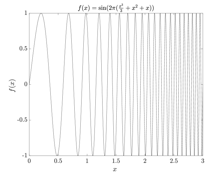
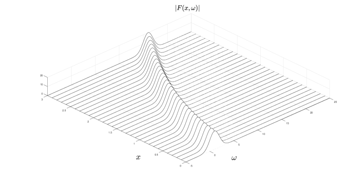
Figure 8 shows the spectrogram for the signal sampled at 100 samples/unit of $x$ (100Hz if $x$ is given in seconds) obtained through Short Time Fourier Transform with Gaussian window function (Gabor Transform Groechenig2001 ) and standard deviation equal to 1. The $\lvert F(x,\omega)\rvert$ values (z-axis) are proportional to the energy in the signal at $(x,\omega)$. For each $x$ (or $\omega$) value there is a range of $\omega$ (or $x$) values whose function $\lvert F(x,\omega)\rvert$ is non-zero. These intervals at $(x,\omega)$ domain represent the uncertainty in determining the instantaneous frequency in this signal representation.

Figure 8: Short Time Fourier Transform - $\lvert F(x,\omega)\rvert$

With:

$$\omega(x)=\omega_{1}x+\omega_{0}$$ (77)

(78) is a Linear Chirp (or Quadratic Phase Signal), with initial frequency $\omega_{0}$ (at $x=0$) and rate chirp $\omega_{1}$:

$$f(x)=\sin\biggl{(}2\pi\biggl{(}\int({\omega_{1}x+\omega_{0}})\,dx\biggr{)}+\phi\biggr{)}=\sin\biggl{(}2\pi\biggl{(}\frac{1}{2}\omega_{1}x^{2}+\omega_{0}x\biggr{)}+\phi\biggr{)}$$ (78)

The resolution of the system,

$$S:\left\{\begin{array}[]{ll}f(x)=\sin\biggl{(}2\pi\biggl{(}\frac{1}{2}\omega_{1}x^{2}+\omega_{0}x\biggr{)}+\phi\biggr{)}\\ f(x+\Delta)=\sin\biggl{(}2\pi\biggl{(}\frac{1}{2}\omega_{1}(x+\Delta)^{2}+\omega_{0}(x+\Delta)\biggr{)}+\phi\biggr{)}\\ f(x+2\Delta)=\sin\biggl{(}2\pi\biggl{(}\frac{1}{2}\omega_{1}(x+2\Delta)^{2}+\omega_{0}(x+2\Delta)\biggr{)}+\phi\biggr{)}\\ \end{array}\right.$$ (79)

applying limit to $\Delta\to 0$, is:

$$\mathfrak{D}\{\omega_{1}\}\frac{df(x)}{dx}=\omega_{1}^{ins}(x)=\lim_{\Delta\to 0}\frac{K_{0}-K_{1}+K_{2}}{2\pi\Delta^{2}}\\$$ (80)

where,

$$K_{0} =\arcsin(f(x))$$

$$K_{1} =\arcsin(2f(x+\Delta))$$

$$K_{2} =\arcsin(f(x+2\Delta))$$

$$\mathfrak{D}\{\omega_{0}\}\frac{df(x)}{dx}=\omega_{0}^{ins}(x)=\lim_{\Delta\to 0}-\frac{1}{2}\frac{K_{0}-K_{1}+K_{2}}{2\pi\Delta^{2}}\\$$ (81)

where,

$$K_{0} =(2x+3\Delta)\arcsin(f(x))$$

$$K_{1} =(4x+4\Delta)\arcsin(f(x+\Delta))$$

$$K_{2} =(2x+\Delta)\arcsin(f(x+2\Delta))$$

$$\mathfrak{D}\{\phi\}\frac{df(x)}{dx}=\phi(x)=\lim_{\Delta\to 0}\frac{1}{2}\frac{K_{0}+K_{1}+K_{2}}{\Delta^{2}}$$ (82)

where,

$$K_{0} =(2\Delta^{2}+x^{2}+3x\Delta)\arcsin(f(x))$$

$$K_{1} =(-2x^{2}-4x\Delta)\arcsin(f(x+\Delta))$$

$$K_{2} =(x^{2}+x\Delta)\arcsin(f(x+2\Delta))$$

According to (77), the instantaneous frequency function is obtained as:

$$\omega(x)=\mathfrak{D}\{\omega 1\}\frac{df(x)}{dx}x+\mathfrak{D}\{\omega_{0}\}\frac{df(x)}{dx}$$ (83)

$\mathfrak{D}\{\omega_{1}\}$, $\mathfrak{D}\{\omega_{0}\}$ ($\mathfrak{D}\{\phi\}$ is not needed in this example) are:

$$\mathfrak{D}\{\omega_{1}\}\frac{df(x)}{dx}=\frac{2\,{\cos\!\left(\frac{2\,\pi\,x\,\left(x^{2}+3\,x+3\right)}{3}\right)}^{3}\,\left(x+1\right)}{{\left({\cos\!\left(\frac{2\,\pi\,x\,\left(x^{2}+3\,x+3\right)}{3}\right)}^{2}\right)}^{\frac{3}{2}}}$$ (84)

$$\mathfrak{D}\{\omega_{0}\}\frac{df(x)}{dx}=-\frac{{\cos\!\left(\frac{2\,\pi\,x\,\left(x^{2}+3\,x+3\right)}{3}\right)}^{3}\,\left(x^{2}-1\right)}{{\left({\cos\!\left(\frac{2\,\pi\,x\,\left(x^{2}+3\,x+3\right)}{3}\right)}^{2}\right)}^{\frac{3}{2}}}$$ (85)

The (84) and (85) have positive and negative values, which are therefore associated with positive and negative frequency values. In absolute values, (84) and (85) are, respectively:

$$\left\lvert{\mathfrak{D}\{\omega_{1}\}\frac{df(x)}{dx}}\right\rvert=\lvert 2x+2\rvert$$ (86)

$$\left\lvert{\mathfrak{D}\{\omega_{0}\}\frac{df(x)}{dx}}\right\rvert=\lvert-x^{2}+1\rvert$$ (87)

However, negative frequency values can be neglected, and therefore the modulus functions at (86) and (87) can be removed without loss of generality. According to (83), the frequency function $\omega_{qr}(x)$ can be reconstructed by:

$$\omega_{qr}(x)=(2x+2)x-x^{2}+1=x^{2}+2x+1$$ (88)

Figure 9: $\omega_{qr}(x)=x^{2}+2x+1$, obtained from $f(x)=\sin\biggl{(}2\pi\biggl{(}\frac{x^{3}}{3}+x^{2}+x\biggr{)}+\phi\biggr{)}$

It is important to note that (88) is obtained from (76) and not from the (60), i.e., the exact instantaneous frequency is obtained from waveform (wave function or signal) ($f(x)$) and not from phase function ($\Omega(x))$ and there is no uncertainty.

Remark.

Heisenberg’s Uncertainty Principle was not respected.

From the instantaneous frequency function $\omega(x)$, the amplitude spectrum $F(\omega)$ can be calculated as:

$$F(\omega)=\frac{1}{\omega}\int_{-\infty}^{\infty}\omega(x)h(x)dx,$$ (89)

with,

$$h(x)=\begin{cases}1\mathchar 24635\relax\;\;\textrm{ if }\omega(x)=\omega\mathchar 24635\relax\;\\ 0\mathchar 24635\relax\;\;\textrm{ otherwise }\\ \end{cases}$$ (90)

6.2 Fourier Derivative

An important exponential function is $e^{-i\omega x}$, with $i=\sqrt{-1}$ and $x,\omega,\in\mathbb{R}$, which is the kernel of the Fourier Transforms Stone2021 . Adding a scaling factor (as in (39)) to this kernel, and proceeding analogously to (41), the Fourier Derivative of function $f(x)$ is:

$$\mathfrak{D}\{\}=e^{-i\omega x+b}$$ (91)

$$\mathfrak{D}\{\omega\}\frac{df(x)}{dx}=\omega(x)=\lim_{\Delta\to 0}\frac{ln(f(x+\Delta))-ln(f(x))}{-i\Delta}$$ (92)

$$\mathfrak{D}\{b\}\frac{df(x)}{dx}=b(x)=\lim_{\Delta\to 0}\frac{ln(f(x))(x+\Delta)-ln(f(x+\Delta))x}{\Delta}$$ (93)

$f(x)$ can be reconstructed from its Fourier derivatives as:

$$f(x)=e^{-i\mathfrak{D}\{\omega\}\frac{df(x)}{dx}x+\mathfrak{D}\{b\}\frac{df(x)}{dx}}$$ (94)

The parameter $\omega$ is the frequency in the kernel of the Fourier Transform, and therefore (92) is the instantaneous frequency ($w(x)\in\mathbb{C}$).

Let $A\in\mathbb{R}$, a wave function of the type $\psi(x,\omega)=Ae^{-i\omega x}$. Considering, as example, $A=2$, $\omega(x)=x^{3}+2x$ (the frequency $\omega$ varies with $x$, i.e. $\omega(x)$) and $\Omega(x)$ the phase function (as in Chirp Signal (74)), the wave function $\psi(x,\omega)$ becomes:

$$\psi(x)=2e^{-i\Omega(x)}=2e^{-i\left(\frac{x^{4}}{4}+x^{2}\right)}$$ (95)

where,

$$\Omega(x)=\int(x^{3}+2x)dx=\left(\frac{x^{4}}{4}+x^{2}\right)$$ (96)

Applying 92 and 93 in 95:

$$\mathfrak{D}\{\omega\}\frac{d\psi(x)}{dx}=\omega(x)=x^{3}+2x$$ (97)

$$\mathfrak{D}\{b\}\frac{d\psi(x)}{dx}=b(x)=i\left(\frac{3x^{4}}{4}+x^{2}\right)+\ln{2}$$ (98)

Applying 94 in 97 and 98, the wave function $\psi(x)$ (95), can be reconstructed as:

$$\psi(x)=e^{-i(x^{3}+2x)x+i\left(\frac{3x^{4}}{4}+x^{2}\right)+\ln{2}}=2e^{-i\left(\frac{x^{4}}{4}+x^{2}\right)}$$ (99)

There is no uncertainty.

Remark.

Heisenberg’s Uncertainty Principle was not respected.

7 Conclusion

In a simplified and summarized manner, Differential Calculus is based on applying a limit tending to zero for Newton’s Difference Quotient applied under any function $f(x)$.

This operation determines another function (the derivative) whose values represent the instantaneous angular coefficients of the tangent lines to the function $f(x)$.

This paper showed that the Differential and Integral Calculus could be applied to other parameters of other functions called derivator and integrator functions.

All the theories presented can be applied to two or more dimensions (partial derivatives and multiple integrals), in addition to well-established operations in classical differential and integral calculus such as the chain rule, product and division derivatives and integrals, differential and integral equations, and others, and this is suggested as future work.

Some examples were presented, with emphasis on the determination of the instantaneous frequency. Although Heisenberg’s Uncertainty Principle is formalized as a property of waves, this paper has shown that uncertainty occurs due to the methodology employed for determining the instantaneous frequency in a function (wave function or signal).

Heisenberg’s Uncertainty Principle is based on the use of integral transforms (such as Fourier Transform and similar wave packets), for a function in the time (or space) domain to obtain its representation in the frequency domain and vice versa.

An integral transform is obviously based on the calculation of integrals. Hence, the integral is suitable for measuring general quantities associated with the whole function domain, such as an area, expected value, norm, autocorrelation, and even frequency distribution (spectral density), but not instantaneous quantities.

Integral transforms (or wave packets) will produce uncertainty in the phase space of canonically conjugate variables.

Nevertheless, why use a mathematical operation based on integral to try to determine instantaneous quantities?

In turn, the derivative is suitable for measuring instantaneous quantities in a function. This paper presented a form to obtain the instantaneous frequency of a function given in the time (or space) domain using derivatives (and not integrals).

The Fourier, Trigonometric, and Chirp Derivatives are examples of different forms to obtain the instantaneous frequency sharply.

References

- \bibcommenthead
- (1) Newton, I.: The Method of Fluxions and Infinite Series - With Its Application to the Geometry of Curve-lines. Henry Woodfall, London (1736)
- (2) Leibniz, G.W.: Nova methodus pro maximis et minimis, itemque tangentibus, quae nec fractas nec irrationales quantitates moratur, et singulare pro illis calculi genus. Acta Eruditorum (XIII), 467–473 (1684)
- (3) Aull, C.E., Chu, S.C., Duncan, R.L., Crow, E.L., Buschman, R.G.: Classroom notes - the first symmetric derivative. The American Mathematical Monthly 74(6), 708–718 (1967). https://doi.org/10.1080/00029890.1967.12000020
- (4) Coleman, R.: Calculus on Normed Vector Spaces. Springer, New York (2012). https://doi.org/10.1007/978-1-4614-3894-6
- (5) Golmankhaneh, A.K.: Fractal Calculus and Its Applications. WORLD SCIENTIFIC, Islamic Azad University (2022). https://doi.org/10.1142/12988
- (6) Chaundy, T.W.: Frank hilton jackson. Journal of the London Mathematical Society s1-37(1), 126–128 (1962). https://doi.org/10.1112/jlms/s1-37.1.126
- (7) Haukkanen, P., , Merikoski, J.K., Tossavainen, T., and: The arithmetic derivative and leibniz-additive functions. Notes on Number Theory and Discrete Mathematics 24(3), 68–76 (2018). https://doi.org/10.7546/nntdm.2018.24.3.68-76
- (8) Kochubei, A.N.: Hypergeometric functions and carlitz differential equations over function fields. In: Arithmetic and Geometry Around Hypergeometric Functions, pp. 163–187. Birkhäuser Basel, Basel (2007). https://doi.org/10.1007/978-3-7643-8284-1_6
- (9) Zuk, J.A.: Covariant-derivative expansion of the effective action and the schwinger-fock gauge condition. Physical Review D 34(6), 1791–1797 (1986). https://doi.org/10.1103/physrevd.34.1791
- (10) Kannan, R., Krueger, C.K.: Dini derivatives. In: Universitext, pp. 55–80. Springer, New York (1996). https://doi.org/10.1007/978-1-4613-8474-8_4
- (11) Tu, L.W.: An Introduction to Manifolds (Universitext), p. 368. Springer, New York (2007)
- (12) Andrews, B., Hopper, C.: The Ricci Flow in Riemannian Geometry. Springer, Berlin (2011). https://doi.org/10.1007/978-3-642-16286-2
- (13) Kac, V., Cheung, P.: q-derivative and h-derivative. In: Quantum Calculus, pp. 1–4. Springer, New York (2002). https://doi.org/10.1007/978-1-4613-0071-7_1
- (14) Hoffmann, D., Kowalski, P.: Integrating hasse–schmidt derivations. Journal of Pure and Applied Algebra 219(4), 875–896 (2015). https://doi.org/10.1016/j.jpaa.2014.05.024
- (15) Lee, J.M.: Lie derivatives. In: Introduction to Smooth Manifolds, pp. 464–493. Springer, New York (2003). https://doi.org/10.1007/978-0-387-21752-9_18
- (16) Mainardi, F., Pagnini, G.: The role of salvatore pincherle in the development of fractional calculus. In: Mathematicians in Bologna 1861–1960, pp. 373–381. Springer, Basel (2011). https://doi.org/10.1007/978-3-0348-0227-7_15
- (17) Xu, D., Jahanchahi, C., Took, C.C., Mandic, D.P.: Enabling quaternion derivatives: the generalized HR calculus. Royal Society Open Science 2(8), 150255 (2015). https://doi.org/10.1098/rsos.150255
- (18) Konstantopoulos, T., Zerakidze, Z., Sokhadze, G.: Radon–nikodým theorem. In: International Encyclopedia of Statistical Science, pp. 1161–1164. Springer, Berlin (2011). https://doi.org/10.1007/978-3-642-04898-2_468
- (19) Luc, D.T., Soleimani-damaneh, M., Zamani, M.: Semi-differentiability of the marginal mapping in vector optimization. SIAM Journal on Optimization 28(2), 1255–1281 (2018). https://doi.org/%****␣annalMathematics.tex␣Line␣1525␣****10.1137/16m1092192
- (20) Rockafellar, R.T., Wets, R.J.B.: Variational Analysis. Springer, Berlin (1998). https://doi.org/10.1007/978-3-642-02431-3
- (21) Lamboni, M.: Weak derivative-based expansion of functions: ANOVA and some inequalities. Mathematics and Computers in Simulation 194, 691–718 (2022). https://doi.org/10.1016/j.matcom.2021.12.019
- (22) Strang, G.: Calculus, p. 615. Wellesley College, Wellesley, MA (1991)
- (23) Jiang, X., Wu, S.: Parameter estimation for chirp signals using the spectrum phase. IET Radar, Sonar & Navigation 14(12), 2039–2044 (2020). https://doi.org/10.1049/iet-rsn.2020.0347
- (24) Born, M.: Physics in My Generation (Heidelberg Science Library), p. 172. Springer, New York (1969)
- (25) Heisenberg, W.: �ber den anschaulichen inhalt der quantentheoretischen kinematik und mechanik. Zeitschrift f�r Physik 43(3-4), 172–198 (1927). https://doi.org/10.1007/bf01397280
- (26) Folland, G.B., Sitaram, A.: The uncertainty principle: A mathematical survey. The Journal of Fourier Analysis and Applications 3(3), 207–238 (1997). https://doi.org/10.1007/bf02649110
- (27) Ford, K.W., Goldstein, D.: The Quantum World, p. 286. Harvard University Press, Boston, MA (2005)
- (28) Hjalmars, S.: Some remarks on time and energy as conjugate variables. Il Nuovo Cimento 25(2), 355–364 (1962). https://doi.org/10.1007/bf02731451
- (29) Louis-Victor-Pierre-Raymond, .Â.d.d.B.: Recherches sur la théorie des quanta. PhD thesis, Sorbonne (1924)
- (30) Rozenman, G.G., Zimmermann, M., Efremov, M.A., Schleich, W.P., Shemer, L., Arie, A.: Amplitude and phase of wave packets in a linear potential. Physical Review Letters 122(12), 124302 (2019). https://doi.org/10.1103/physrevlett.122.124302
- (31) Schlosshauer, M.: Decoherence, the measurement problem, and interpretations of quantum mechanics. Reviews of Modern Physics 76(4), 1267–1305 (2005). https://doi.org/10.1103/revmodphys.76.1267
- (32) Giacosa, F.: On unitary evolution and collapse in quantum mechanics. Quanta 3(1), 156 (2014). https://doi.org/10.12743/quanta.v3i1.26
- (33) Born, M.: Zur quantenmechanik der sto�vorg�nge. Zeitschrift f�r Physik 37(12), 863–867 (1926). https://doi.org/10.1007/bf01397477
- (34) Stone, J.V.: The Fourier Transform. Tutorial Introductions, Sebtel (2021). https://www.ebook.de/de/product/40714450/james_v_stone_the_fourier_transform.html
- (35) Zhou, L.: Cauchy–schwarz inequality for differences revisited. The American Mathematical Monthly 129(1), 65–65 (2021). https://doi.org/10.1080/00029890.2022.1994256
- (36) Choe, H.: On the justification and validity of the kennard inequality. American Journal of Modern Physics 9(5), 73 (2020). https://doi.org/10.11648/j.ajmp.20200905.12
- (37) Gröchenig, K.: The short-time fourier transform. In: Foundations of Time-Frequency Analysis, pp. 37–58. Birkhäuser Boston, Boston (2001). https://doi.org/10.1007/978-1-4612-0003-1_4
- (38) Strang, G.: Wavelets and Filter Banks. Wellesley-Cambridge Press, Wellesley, MA (1996)
- (39) Hlawatsch, F.: The Wigner Distribution, p. 459. Elsevier, Amsterdan (1997)
- (40) Gretinger, M., Secara, M., Festila, C., Dulf, E.H.: Signal generators for frequency response experiments. In: 2014 IEEE International Conference on Automation, Quality and Testing, Robotics. IEEE, Cluj-Napoca, Romania (2014). https://doi.org/10.1109/aqtr.2014.6857860