Three components of stochastic entropy production associated with the quantum Zeno and anti-Zeno effects

Abstract

We investigate stochastic entropy production in a two-level quantum system that performs Rabi oscillations while undergoing quantum measurement brought about by continuous random disturbance by an external measuring device or environment. The dynamics produce quantum Zeno and anti-Zeno effects for certain measurement regimes, and the stochastic entropy production is a measure of the irreversibility of the behaviour. When the strength of the measurement disturbance is time-dependent, the stochastic entropy production separates into three components. Two represent relaxational behaviour, one being specific to systems represented by coordinates that are odd under time reversal symmetry, and a third characterises the nonequilibrium stationary state arising from breakage of detailed balance in the dynamics. The study illustrates how the ideas of stochastic thermodynamics may be applied in similar ways to both quantum and classical systems.

I Introduction

Entropy quantifies subjective uncertainty in the configuration of a system and it can be argued that similar applications of this concept should apply in both classical and quantum mechanics, where configurations are described by phase space coordinates and by elements of a density matrix, respectively. The effective stochastic dynamics of such variables brought about by coupling the system to a coarse grained environment will increase the configurational uncertainty of the world (the system together with its environment) as time passes. Such a loss of information is often manifested in the dispersal of energy and matter or the loss of correlations: consequences of the chaotic nature of the underlying deterministic dynamics but nevertheless captured by stochastic modelling. This is the content of the second law of thermodynamics [1].

The aim of this paper is to compute the stochastic entropy production and hence loss of information when a simple quantum system undergoing Rabi oscillations is subjected to continuous measurement of two non-commuting observables [2]. The system exhibits Zeno and anti-Zeno effects [3] depending on the relative strengths of the two measurement processes. It is of particular interest to consider the division of the stochastic entropy production into three components when the strength of measurement is time-dependent [4, 5]. Each component describes an aspect of the nonequilibrium, irreversible behaviour of the system.

In Section II we derive Markovian stochastic differential equations, or Itô processes, that describe the evolution of the system. We examine Zeno and anti-Zeno effects where the mean rate of change of a system coordinate is reduced or increased, respectively, when measurement is made more intense. The nature of the three components of stochastic entropy production for time-dependent measurement of one of the observables is discussed in Section III. We give our conclusions in Section IV.

II Stochastic dynamics

The reduced density matrix $\rho$ is a specification of the state of an open quantum system and under certain conditions of coupling to the environment its evolution can be modelled using a stochastic Lindblad equation:

$$d\rho =-i[H,\rho]dt+\sum_{i}\left(c_{i}\rho c_{i}^{\dagger}-\frac{1}{2}\rho c_{i}^{\dagger}c_{i}-\frac{1}{2}c_{i}^{\dagger}c_{i}\rho\right)dt$$

$$\qquad+\left(\rho c_{i}^{\dagger}+c_{i}\rho-C_{i}\rho\right)dW_{i},$$ (1)

with $C_{i}={\rm Tr}\left((c_{i}+c_{i}^{\dagger})\rho\right)$, where $H$ is the system Hamiltonian. The Lindblad operators $c_{i}$ represent the modes of interaction between the system and the environment, and the $dW_{i}$ are a set of independent Wiener increments [6, 7, 8]. This framework is a form of quantum state diffusion, where evolution of $\rho$ is continuous, without jumps [9].

We consider a two-level bosonic system represented by $\rho=\frac{1}{2}\left(\mathbb{I}+\boldsymbol{r}\cdot\boldsymbol{\sigma}\right)$, where $\boldsymbol{r}$ is the coherence or Bloch vector and $\sigma_{k}$ are the Pauli matrices, with $H=\epsilon\sigma_{z}$, $c_{1}=\alpha_{x}\sigma_{x}$ and $c_{2}=\alpha_{y}\sigma_{y}$. The dynamics describe a system that performs Rabi oscillations in the expectation values $r_{x}={\rm Tr}(\sigma_{x}\rho)$ and $r_{y}={\rm Tr}(\sigma_{y}\rho)$ when isolated, but which departs stochastically from such regular behaviour when the coupling coefficients $\alpha_{x}$ and $\alpha_{y}$ are non-zero. The situation is similar to a two-level system undergoing the measurement of one observable, studied previously [10].

The Lindblads $c_{1}$ and $c_{2}$ tend to drive the system towards eigenstates of $\sigma_{x}$ and $\sigma_{y}$, respectively, and their use in Eq. (1) can be regarded as an implementation of the continuous, simultaneous measurement of these two system observables [7]. The coefficients $\alpha_{x}$ and $\alpha_{y}$ are measurement strengths, since increasing $\alpha_{x}$ while $\alpha_{y}$ is held constant brings about a greater concentration of the pdf in the vicinity of the eigenstates of $\sigma_{x}$, and vice versa.

The dynamics of the components of $\boldsymbol{r}$ can be expressed as Itô processes:

$$dr_{x} \!=\!-2\left(\epsilon r_{y}+\alpha_{y}^{2}r_{x}\right)\!dt+2\alpha_{x}\left(1-r_{x}^{2}\right)\!dW_{x}\!-\!2\alpha_{y}r_{x}r_{y}dW_{y}$$

$$dr_{y} \!=\!2\left(\epsilon r_{x}-\alpha_{x}^{2}r_{y}\right)\!dt-2\alpha_{x}r_{x}r_{y}dW_{x}+2\alpha_{y}\left(1-r_{y}^{2}\right)\!dW_{y}$$

$$dr_{z} \!=\!-2r_{z}\left(\alpha_{x}^{2}+\alpha_{y}^{2}\right)\!dt-2r_{z}\left(\alpha_{x}r_{x}dW_{x}+\alpha_{y}r_{y}dW_{y}\right),$$ (2)

where $dW_{x}$ and $dW_{y}$ are Wiener increments.

We consider a (pure) state denoted by $r_{z}=0$, $r_{x}=\sin\phi$ and $r_{y}=\cos\phi$. The coherence vector lies in the equatorial plane of the Bloch sphere and its rotation about the $r_{z}$ axis is specified by an azimuthal angle $\phi=\tan^{-1}(r_{x}/r_{y})$. The stochastic evolution of $\phi$ can be derived from Eq. (2) using Itô’s lemma:

$$d\phi =\left(2\epsilon-\left(\alpha_{x}^{2}-\alpha_{y}^{2}\right)\sin 2\phi\right)dt$$

$$-2\alpha_{x}\sin\phi\,dW_{x}+2\alpha_{y}\cos\phi\,dW_{y}$$

$$= \left(2\epsilon-\left(\alpha_{x}^{2}-\alpha_{y}^{2}\right)\sin 2\phi\right)dt$$

$$-2\left(\alpha_{x}^{2}\sin^{2}\phi+\alpha_{y}^{2}\cos^{2}\phi\right)^{1/2}dW,$$ (3)

where $dW$ is also a Wiener increment. The dynamics produce a linear increase in $\phi$ with time when the system is isolated ($\alpha_{x}=\alpha_{y}=0$). This drift is distorted by random disturbances when the system is coupled to the environment, here regarded as a measuring device. The associated Fokker-Planck equation for the probability density function (pdf) $p(\phi,t)$ is

$$\frac{\partial p(\phi,t)}{\partial t} =-\frac{\partial J}{\partial\phi},$$ (4)

where the probability current is

$$J =\left(2\epsilon-\left(\alpha_{x}^{2}-\alpha_{y}^{2}\right)\sin 2\phi\right)p(\phi,t)$$

$$-2\frac{\partial}{\partial\phi}\left(\alpha_{x}^{2}\sin^{2}\phi+\alpha_{y}^{2}\cos^{2}\phi\right)p(\phi,t).$$ (5)

The situation with equal non-zero measurement strengths $\alpha_{x}=\alpha_{y}=\alpha\neq 0$ is described by $d\phi=2\epsilon dt-2\alpha dW$. The system then evolves towards a stationary state with $p_{{\rm st}}(\phi)=(2\pi)^{-1}$ and $J=\epsilon/\pi$. When $\alpha_{x}\neq\alpha_{y}$, there is also a stationary state with constant $J$ but characterised by a nonuniform pdf. These are nonequilibrium situations with consequent stochastic entropy production, which we investigate in the next section.

We consider the dependence of the mean rate of change of $\phi$ on the measurement strengths $\alpha_{x}$ and $\alpha_{y}$. The mean of $\phi$ evolves according to

$$\frac{d\langle\phi\rangle}{dt}=2\epsilon-\left(\alpha_{x}^{2}-\alpha_{y}^{2}\right)\langle\sin 2\phi\rangle,$$ (6)

where the angled brackets represent an average over the stochasticity. Results from numerical simulations of Eq. (3) are given in Figure 1 for $\epsilon=1/2$, $\alpha_{x}=1$ and a range of values of $\alpha_{y}$. The Zeno effect operates for $\alpha_{y}>\alpha_{x}$; a slowing of the average evolution of the system as the strength of measurement $\alpha_{y}$ is increased at a constant $\alpha_{x}$ [10]. There is also an anti-Zeno effect for $\alpha_{y}<\alpha_{x}$, where the mean evolution is speeded up when $\alpha_{y}$ is increased. For $\alpha_{x}=\alpha_{y}$ and $p_{{\rm st}}(\phi)=(2\pi)^{-1}$ the average of $\sin 2\phi$ vanishes, and $d\langle\phi\rangle/dt=2\epsilon$: the effects of the two measurement processes on the mean rate of Rabi oscillation then cancel each other out, somewhat counter-intuitively.

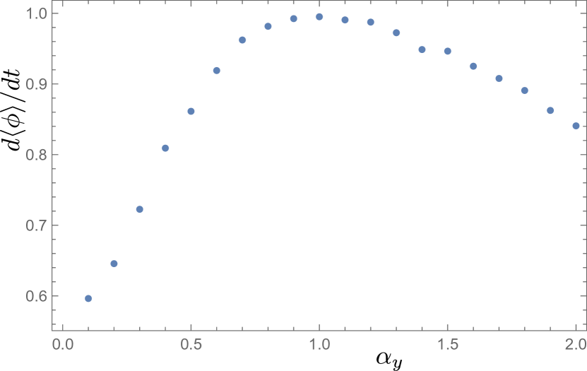
Figure 1: Zeno and anti-Zeno effects are apparent in the mean rate of Rabi oscillations, arising from changing the measurement strength $\alpha_{y}$ for $\alpha_{x}=1$ and $\epsilon=1/2$. The average is obtained over a time interval $\Delta t=10^{5}$ for each value of $\alpha_{y}$ and the error in the mean is estimated to be less than 0.01.

III Stochastic entropy production

We now consider the stochastic thermodynamics associated with the dynamics

$$d\phi=\left(A^{{\rm rev}}(\phi)+A^{{\rm irr}}(\phi)\right)dt+B(\phi,t)dW,$$ (7)

where the terms involving $A^{{\rm rev}}$ and $A^{{\rm irr}}$ represent deterministic rates of change of $\phi$ that satisfy and violate time reversal symmetry, respectively. The stochastic entropy production is given by [5]

$$d\Delta s_{{\rm tot}} = -d\ln p(\phi,t)+\frac{A^{{\rm irr}}}{D}d\phi-\frac{A^{{\rm rev}}A^{{\rm irr}}}{D}dt+\frac{dA^{{\rm irr}}}{d\phi}dt$$ (8)

$$-\frac{dA^{{\rm rev}}}{d\phi}dt-\frac{1}{D}\frac{\partial D}{\partial\phi}d\phi+\frac{(A^{{\rm rev}}-A^{{\rm irr}})}{D}\frac{\partial D}{\partial\phi}dt$$

$$-\frac{\partial^{2}D}{\partial\phi^{2}}dt+\frac{1}{D}\left(\frac{\partial D}{\partial\phi}\right)^{2}dt,$$

where $D(\phi,t)=\frac{1}{2}B(\phi,t)^{2}$. For dynamics that possess an equilibrium state (a stationary state with vanishing probability current $J$) characterised by a pdf $p_{{\rm st}}(\phi)$, Eq. (8) reduces to the simpler expression $d\Delta s_{{\rm tot}}=-d\ln\left(p(\phi,t)/p_{{\rm st}}(\phi)\right)$, showing explicitly how stochastic entropy production can arise from a statistical deviation from equilibrium. The system under consideration here, however, does not possess an equilibrium state in general, but instead a nonequilibrium stationary state with non-zero $J$.

For bosonic systems, the time reversal operation corresponds to taking a complex conjugate of the density matrix. Thus the components $r_{x}$ and $r_{z}$ of the coherence vector are even and the component $r_{y}$ is odd under time reversal symmetry. This means that $\phi$ is also odd and we deduce that $A^{{\rm rev}}=2\epsilon$ and $A^{{\rm irr}}=-\left(\alpha_{x}^{2}-\alpha_{y}^{2}\right)\sin 2\phi$. The diffusion coefficient is $D=2\left(\alpha_{x}^{2}\sin^{2}\phi+\alpha_{y}^{2}\cos^{2}\phi\right)$. We take the coefficients $\alpha_{x}$ and $\alpha_{y}$ to be time-independent (for now) and write $dA^{{\rm irr}}/d\phi=-2\left(\alpha_{x}^{2}-\alpha_{y}^{2}\right)\cos 2\phi$, $dD/d\phi=2\left(\alpha_{x}^{2}-\alpha_{y}^{2}\right)\sin 2\phi$, $d^{2}D/d\phi^{2}=4\left(\alpha_{x}^{2}-\alpha_{y}^{2}\right)\cos 2\phi$, and obtain

$$d\Delta s_{{\rm tot}}=-d\ln p+\frac{9\left(\alpha_{x}^{2}-\alpha_{y}^{2}\right)^{2}\sin^{2}2\phi}{2\left(\alpha_{x}^{2}\sin^{2}\phi+\alpha_{y}^{2}\cos^{2}\phi\right)}dt$$

$$- 6\left(\alpha_{x}^{2}-\alpha_{y}^{2}\right)\cos 2\phi dt+\frac{3\left(\alpha_{x}^{2}-\alpha_{y}^{2}\right)\sin 2\phi}{\left(\alpha_{x}^{2}\sin^{2}\phi+\alpha_{y}^{2}\cos^{2}\phi\right)^{1/2}}dW.$$ (9)

For $\alpha_{y}=0$, and hence measurement of $\sigma_{x}$ alone, this reduces to

$$d\Delta s_{{\rm tot}}=-d\ln p+6\alpha_{x}^{2}\left(1+\cos^{2}\phi\right)dt+6\alpha_{x}\cos\phi\,dW,$$ (10)

and we conclude that in a stationary state, for a given value of $\alpha_{x}$, the stochastic entropy production increases on average at a constant rate given by

$$\frac{d\langle\Delta s_{{\rm tot}}\rangle}{dt}=6\alpha_{x}^{2}\left(1+\langle\cos^{2}\phi\rangle\right),$$ (11)

since $\langle-d\ln p\rangle=dS_{G}=0$ in these circumstances, where $S_{G}=-\int p\ln p\,d\phi$ is the Gibbs entropy. For larger $\alpha_{x}^{2}$, the pdf becomes more concentrated in the region of $\phi=0$ and $\pi$, corresponding to the eigenstates of $\sigma_{x}$ [10], such that $\langle\cos^{2}\phi\rangle$ increases with $\alpha_{x}^{2}$ towards an upper limit of unity. Thus a increase in measurement strength brings about a higher mean rate of production of stochastic entropy, which can be associated intuitively with the increased Zeno slowing down, on average, of the Rabi oscillations.

We now consider a situation where the measurement strength $\alpha_{x}$ is time-dependent. In such circumstances the stochastic entropy production separates into three identifiable components [5], written

$$d\Delta s_{{\rm tot}}=d\Delta s_{1}+d\Delta s_{2}+d\Delta s_{3}.$$ (12)

The rate of change of the mean value of the first component may be written in the form

$$\frac{d\langle\Delta s_{1}\rangle}{dt}=-\int\frac{\partial p}{\partial t}\ln\frac{p(\phi,t)}{p_{{\rm st}}^{\alpha_{x}}(\phi)}d\phi.$$ (13)

Evidently, this is a relaxational entropy production that vanishes when the system is in a stationary state characterised by the pdf $p_{{\rm st}}^{\alpha_{x}}(\phi)$ associated with a specified value of $\alpha_{x}$. Esposito and Van den Broeck denoted this component the nonadiabatic entropy production [11]. Its mean rate of change can never be negative.

We solve the Fokker-Planck equation for $\epsilon=10$ and a range of values of $\alpha_{x}$ (with $\alpha_{y}=0$) to obtain stationary pdfs $p_{{\rm st}}^{\alpha_{x}}(\phi)$. We then introduce a time-dependent measurement strength $\alpha_{x}=2+\sin 20\pi t$ to obtain a time-dependent pdf $p(\phi,t)$ that settles into a periodic stationary state, as shown in Figure 2. The principal feature to notice is that the system is periodically attracted, statistically speaking, towards the eigenstates of the $\sigma_{x}$ observable at $\phi=0$ and $\pi$, though displaced to higher values by the Rabi rotation.

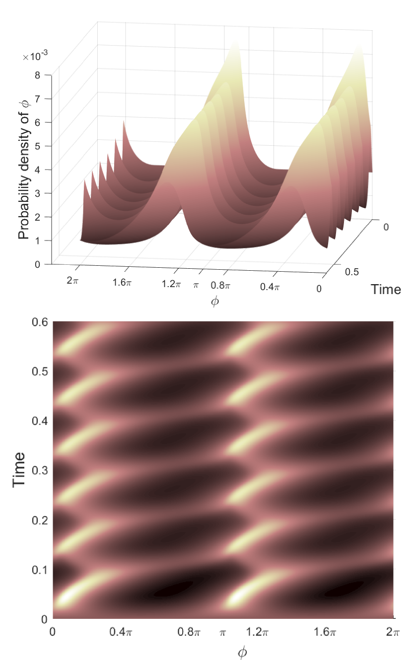
Figure 2: Probability density function for $\phi$ against time (side and top views) brought about by competition between a time-dependent measurement strength $\alpha_{x}=2+\sin 20\pi t$ that draws the system towards eigenstates of $\sigma_{x}$ at $\phi=0$ and $\pi$, and Rabi oscillations characterised by $\epsilon=10$ that favour a positive drift for $\phi$.

We have calculated the average of $\Delta s_{1}$ as a function of time for $\epsilon=10$ and $\alpha_{x}=2+\sin 20\pi t$ using methods described in [5] and the results are given in Figure 3. Since the system is prevented from reaching a stationary state through the time-dependence of the measurement strength, the mean rate of change of this component of stochastic entropy production never falls to zero, but instead continues to evolve periodically.

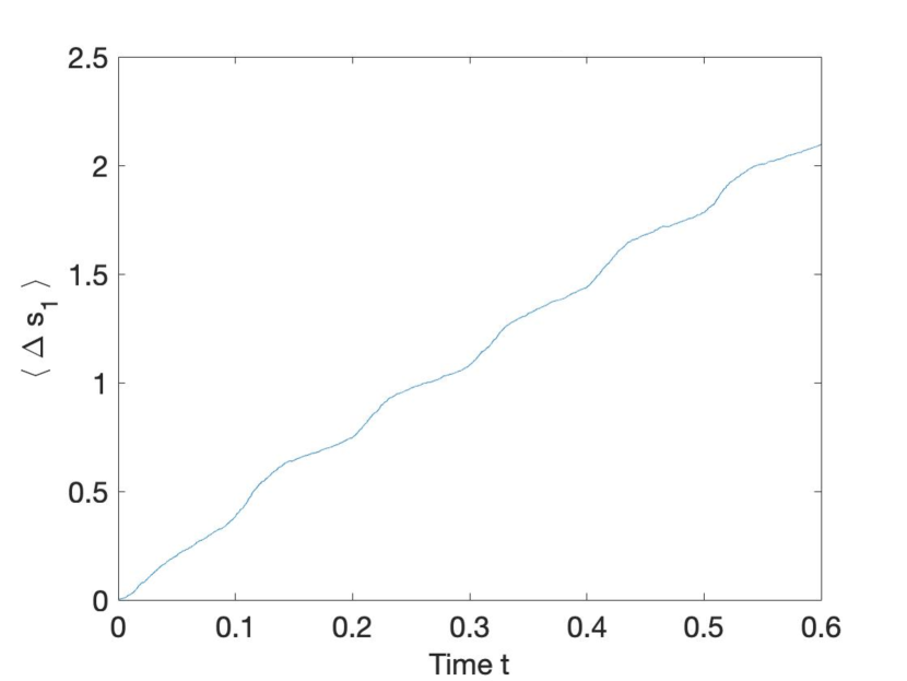
Figure 3: The average of $\Delta s_{1}$, the nonadiabatic component of stochastic entropy production, evolving with time, for $\alpha_{x}=2+\sin 20\pi t$, $\alpha_{y}=0$ and $\epsilon=10$, adopting a periodic stationary state to accompany the Zeno slowing down of the Rabi oscillations and reflecting the time-dependence of the measurement strength $\alpha_{x}$.

The average of the second component of stochastic entropy production evolves according to [4]

$$\frac{d\langle\Delta s_{2}\rangle}{dt}=\int\frac{p}{D}\left(\frac{J_{{\rm st}}^{{\rm irr}}(\phi^{{\rm T}})}{p_{{\rm st}}^{\alpha_{x}}(\phi^{{\rm T}})}\right)^{2}d\phi,$$ (14)

where $\phi^{{\rm T}}$ is the transform of $\phi$ under time reversal: since $\phi$ is odd, $\phi^{{\rm T}}=-\phi$. $\Delta s_{2}$ is a contribution to stochastic entropy production arising from the breakage of detailed balance, which permits the emergence of a non-zero irreversible probability current in a stationary state, given by

$$J_{{\rm st}}^{{\rm irr}}(\phi)=A^{{\rm irr}}p_{{\rm st}}^{\alpha_{x}}(\phi)-\frac{\partial}{\partial\phi}D(\phi,\alpha_{x})p_{{\rm st}}^{\alpha_{x}}(\phi),$$ (15)

where the diffusion coefficient is specified by the current value of $\alpha_{x}$. Esposito and Van den Broeck referred to $\Delta s_{2}$ as the adiabatic entropy production [11] and Spinney and Ford, who included a consideration of dynamical variables that are odd as well as even under time reversal symmetry, denoted it the generalised housekeeping entropy production [4]. Like the nonadiabatic entropy production, its mean rate of change is never negative. The evolution of $\langle\Delta s_{2}\rangle$ for $\epsilon=10$ and $\alpha_{x}=2+\sin 20\pi t$ is illustrated in Figure 4.

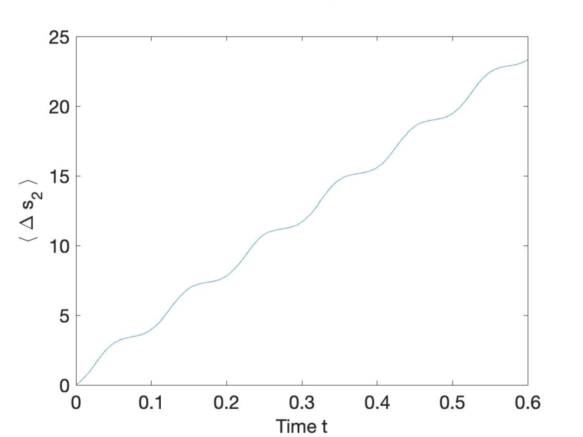
Figure 4: Average of $\Delta s_{2}$, the adiabatic component of stochastic entropy production, against time, for $\alpha_{x}=2+\sin 20\pi t$, $\alpha_{y}=0$ and $\epsilon=10$.

The average rate of change of the third contribution to the stochastic entropy production may be written

$$\frac{d\langle\Delta s_{3}\rangle}{dt}=-\int\frac{\partial p}{\partial t}\ln\frac{p_{{\rm st}}^{\alpha_{x}}(\phi)}{p_{{\rm st}}^{\alpha_{x}}(\phi^{{\rm T}})}d\phi.$$ (16)

$\Delta s_{3}$ is a contribution associated with relaxation towards a stationary state and in this respect is similar to $\Delta s_{1}$. It explicitly vanishes when there are no odd variables in the dynamics, but here it does not vanish. It was designated the transient housekeeping entropy production by Spinney and Ford [4]. The evolution of $\langle\Delta s_{3}\rangle$ for $\epsilon=10$ and $\alpha_{x}=2+\sin 20\pi t$ is illustrated in Figure 5. Notice that a negative mean rate of production is permitted, in contrast to the other two contributions. The mean rate of change of $\Delta s_{{\rm tot}}$ is, of course, positive for all times, in accordance with the second law [12].

If we were to re-introduce the measurement of $\sigma_{y}$, and hence create conditions for an anti-Zeno effect in the dynamics, the stochastic entropy production would similarly divide into three components and quantify the relative contributions of different sources of irreversibility.

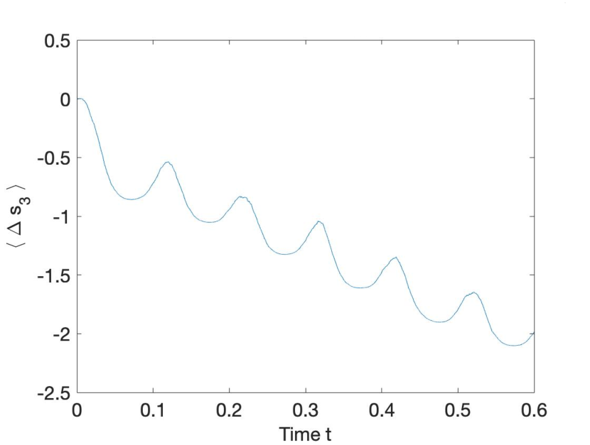
Figure 5: Average of $\Delta s_{3}$, the transient housekeeping stochastic entropy production, against time, for $\alpha_{x}=2+\sin 20\pi t$, $\alpha_{y}=0$ and $\epsilon=10$.

IV Conclusions

Employing the framework of quantum state diffusion as a model of the evolution of an open quantum system allows us to investigate the effect of measurement on the intrinsic dynamics of a quantum system. We have previously investigated a Zeno effect in a multi-level bosonic system: a slowing down of Rabi oscillations, on average, when measurements are performed to determine the level currently occupied [10]. Here we extend that study to demonstrate that simultaneous measurement of a second, non-commuting observable can produce a counter-intuitive anti-Zeno effect, specifically that the slowed down evolution can be speeded up when measurement of the second observable is introduced.

The principal aim of the study, however, has been to compute the stochastic entropy production associated with the evolution of a two-level system when a Zeno effect is operating as a result of the continuous measurement of one observable. Our investigation of the division of the stochastic entropy production into its three components is motivated by a wish to demonstrate that the ideas underpinning stochastic thermodynamics can apply with equal validity to classical and quantum mechanics. Stochastic entropy production measures the irreversibility of the evolution of a system when subjected to unpredictable external disturbance. This is the extent to which two sequences of events, one the reverse of the other, occur with different probabilities in such circumstances. We take the trajectory followed by the reduced density matrix of an open quantum system, when it is subjected to continuous measurement, to be analogous to the Brownian path of a classical particle under the influence of an unpredictable environment. Irreversibility occurs in both situations and can be quantified.

The division of stochastic entropy production into components demonstrates how irreversibility can be associated with the relaxation of a system towards stationarity (components $\Delta s_{1}$ and $\Delta s_{3}$) and with the breakage of detailed balance and the consequent existence of a nonequilibrium stationary state (component $\Delta s_{2}$). These three contributions emerge in the two-level quantum system when we make the strength of measurement a periodic function of time, such that the reduced density matrix and the mean stochastic entropy production also evolve periodically. We conclude that stochastic entropy production associated with nonequilibrium behaviour, reflecting a continuing loss of information concerning the configuration of the world, can be demonstrated in open quantum systems as well as in classical situations.