Covariant derivatives of Berry-type quantities: Application to nonlinear transport

Abstract

The derivatives of the Berry curvature $\Omega$ and intrinsic orbital magnetic moment ${\bf m}$ in momentum space are relevant to various problems, including the nonlinear anomalous Hall effect and magneto-transport within the Boltzmann-equation formalism. To investigate these properties using first-principles methods, we have developed a Wannier interpolation scheme that evaluates the “covariant derivatives” of the non-Abelian $\Omega$ and ${\bf m}$ matrices for a group of bands within a specific energy range of interest. Unlike the simple derivative, the covariant derivative does not involve couplings within the groups and preserves the gauge covariance of the $\Omega$ and ${\bf m}$ matrices. In the simulation of nonlinear anomalous Hall conductivity, the resulting “Fermi-sea” formula for the Berry curvature dipole are more robust and converges faster with the density of the integration k-grid than the “Fermi-surface” formula implemented earlier. The developed methodology is made available via the open-source code WannierBerri and we demonstrate the efficiency of this method through first-principles calculations on trigonal Tellurium.

I Introduction

The absence of spatial inversion and/or time-reversal symmetry gives rise to various nonlinear transport phenomena in solids Tokura and Nagaosa (2018), including unidirectional magnetoresistance Rikken et al. (2001); Avci et al. (2015) and nonlinear Hall effects Deyo et al. (2009); Sodemann and Fu (2015); Ma et al. (2019); Kang et al. (2019); Huang et al. (2020); Zhang et al. (2020). Such effects are encoded in the expansion of the current density in powers of the applied electric and magnetic fields,

$$j_{a} =\sigma^{10}_{ab}E_{b}+\sigma^{11}_{ab\alpha}E_{b}B_{\alpha}+\sigma^{12}_{ab\alpha\beta}E_{b}B_{\alpha}B_{\beta}$$

$$+\sigma^{20}_{abc}E_{b}E_{c}+\sigma^{21}_{abc\alpha}E_{b}E_{c}B_{\alpha}$$

$$+\sigma^{30}_{abcd}E_{b}E_{c}E_{d}$$

$$+\ldots\,.$$ (1)

At low frequencies, the expansion coefficients can be evaluated using semiclassical Xiao et al. (2010); Gao (2019) as well as fully quantum-mechanical methods Morimoto et al. (2016); Watanabe and Yanase (2020). The resulting expressions contain two types of terms: (i) intraband terms that only involve intrinsic geometric properties of the unperturbed Bloch states (Berry curvature, effective mass, magnetic moment, and quantum metric); (ii) interband terms that take into account how the Bloch states change, via vertical band mixing, under the applied fields Gao (2019).

This paper deals with the evaluation of intraband nonlinear conductivities, which typically contain derivatives of geometric quantities with respect to crystal momentum ${\bf k}$. While the focus will be on ab initio implementations based on Wannier functions, the formalism presented here can also be combined with effective-Hamiltonian methods such as ${\bf k}\cdot{\bf p}$ and tight-binding.

Consider the current response at zero magnetic field,

$$j_{a}=\sigma^{10}_{ab}E_{b}+\sigma^{20}_{abc}E_{b}E_{c}+\sigma^{30}_{abcd}E_{b}E_{c}E_{d}+\ldots$$ (2)

Working in the constant relaxation time approximation and neglecting interband contributions, one obtains Zhang et al. (2020)

$$\sigma^{10}_{ab} =\frac{e^{2}}{\hbar}\int[d{\bf k}]\sum_{n}\,f_{0}(\varepsilon_{{\bf k}n})\left[(\tau/\hbar)\partial^{2}_{ab}\varepsilon_{{\bf k}n}-\Omega^{ab}_{{\bf k}n}\right]\,,$$ (3)

$$\sigma^{20}_{abc} =\frac{e^{3}\tau}{\hbar^{2}}\int[d{\bf k}]\sum_{n}\,f_{0}(\varepsilon_{{\bf k}n})\left[-(\tau/\hbar)\partial^{3}_{abc}\varepsilon_{{\bf k}n}+\partial_{c}\Omega^{ab}_{{\bf k}n}\right]\,,$$ (4)

$$\sigma^{30}_{abcd} =\frac{e^{4}\tau^{2}}{\hbar^{3}}\int[d{\bf k}]\sum_{n}\,f_{0}(\varepsilon_{{\bf k}n})\bigg{(}(\tau/\hbar)\partial^{4}_{abcd}\varepsilon_{{\bf k}n}$$

$$\,\,\,\,\,\,\,\,\,\,\,\,\,\,\,\,\,\,\,\,\,\,\,\,\,\,\,\,\,\,\,\,\,\,\,\,\,\,\,\,\,\,\,\,\,\,\,\,-\frac{3}{4}\partial^{2}_{cd}\Omega^{ab}_{{\bf k}n}-\frac{1}{4}\partial^{2}_{bc}\Omega^{ad}_{{\bf k}n}\bigg{)}\,.$$ (5)

where $\tau$ is the relaxation time, $[d{\bf k}]\equiv d^{3}k/(2\pi)^{3}$, $\partial_{a}\equiv\partial/\partial k_{a}$, and the integrals are over the first Brillouin zone (BZ). The band energy is denoted $\varepsilon_{{\bf k}n}$, $f_{0}(\varepsilon_{{\bf k}n})$ is the Fermi-Dirac distribution function, and

$$\Omega^{ab}_{{\bf k}n}=-2\mathrm{Im}\langle\partial_{a}u_{{\bf k}n}|\partial_{b}u_{{\bf k}n}\rangle$$ (6)

is the Berry curvature, where $|u_{{\bf k}n}\rangle$ is the periodic part of a Bloch state $|\psi_{{\bf k}n}\rangle$. Equations (3-5) are written in the so-called ”Fermi-sea” form, meaning that all states below the Fermi level contribute to the integral.

Equation (3) gives the linear conductivity: the first term is the Ohmic Drude conductivity expressed in terms of the inverse effective mass of the occupied states; the second term, given by the net Berry curvature of the occupied states, describes an intrinsic anomalous Hall effect in magnetic conductors Nagaosa et al. (2010). Equation (4) gives the quadratic conductivity: the first term is Ohmic and it describes unidirectional magnetoresistance in magnetic acentric conductors Železný et al. (2021), while the second term describes an anomalous Hall effect in nonmagnetic acentric conductors Deyo et al. (2009); Sodemann and Fu (2015); Ma et al. (2019); Kang et al. (2019). Equation (5) describes cubic Ohmic and anomalous Hall responses, which so far have only been studied theoretically Parker et al. (2019); Zhang et al. (2020). Note that higher-order conductivities contain higher-order derivatives of the band dispersion and of the Berry curvature. For magnetoconductivities such as $\sigma^{11}_{ab\alpha}$, $\sigma^{12}_{ab\alpha\beta}$ and $\sigma^{21}_{abc\alpha}$ in Eq. (1), the intrinsic magnetic moment and its derivatives are needed as well Xiao et al. (2010); Gao (2019); Morimoto et al. (2016); Lahiri et al. (2022).

The first-principles evaluation of both terms in the linear conductivity (3) is by now a fairly routine task. A popular approach is Wannier interpolation Wang et al. (2006); Yates et al. (2007), where a Slater-Koster type of interpolation is carried out for the quantities of interest after mapping the low-energy ab initio electronic structure onto a basis of localized Wannier functions.

When it comes to nonlinear conductivities, ab initio calculations are still quite recent. In the case of intraband responses such as Eqs. (4) and (5), a possible strategy is as follows. First compute the inverse effective mass and Berry curvature on a dense ${\bf k}$ mesh by Wannier interpolation, and then evaluate their ${\bf k}$ derivatives by finite differences. This strategy was used in several recent studies of nonlinear anomalous Hall effects Zhang et al. (2018a, b, 2020); He and Weng (2021).

Another common strategy is to employ integration by parts in Eqs. (4-5) and thus transfer the derivative from the Berry curvature $\Omega^{ab}_{{\bf k}n}$ to the Fermi-Dirac distribution $f_{0}(\varepsilon_{{\bf k}n})$. For instance, the second term of Eq. (4) is governed by the so-called ”Berry curvature dipole” Sodemann and Fu (2015) which in the Fermi-sea formulation is given by

$$\mathcal{D}_{cd}^{\rm sea}=\epsilon_{abd}\int[d{\bf k}]\sum_{n}\partial_{c}\Omega_{{\bf k}n}^{ab}f_{0}(\varepsilon_{{\bf k}n})~{},$$ (7)

Using integration by parts it may be rewritten in as

$$\mathcal{D}_{cd}^{\rm surf}=\epsilon_{abd}\int[d{\bf k}]\sum_{n}\Omega_{{\bf k}n}^{ab}\partial_{c}\varepsilon_{{\bf k}n}\left(-\frac{\partial f_{0}}{\partial\varepsilon}\right)_{\varepsilon=\varepsilon_{{\bf k}n}}~{},$$ (8)

At low temperature the derivative of the distribution function $f_{0}^{\prime}$ is a narrow peak, which ensures that only electronic states that are close to the Fermi level contribute to the integral. Therefore, such formulations are called “Fermi-surface” integrals. As we will show, in numerical simulations, such integrals require denser sampling of the Brillouin zone, compared to the “Fermi-sea” integrals. Moreover, for magnetoconductivities magnetoconductivities such as $\sigma^{11}_{ab\alpha}$, $\sigma^{12}_{ab\alpha\beta}$ and $\sigma^{21}_{abc\alpha}$ it is not always possible to get rid of derivatives of Berry curvature and orbital magnetic moment simultaneously.

In this work, we develop an alternative approach where derivatives of geometric quantities are evaluated perturbatively, without resorting to finite differences. Importantly, the expressions we obtain are oblivious to band crossings and avoided crossings away from the Fermi level, as expected on physical grounds. We emphasize that this is not the case if one differentiates the Berry curvature in a naive way: the resulting expression contains spurious terms that react strongly to remote level crossings (see for example Ref. Morimoto et al. (2016)). To obtain well-behaved gradient formulas we start from gauge-covariant matrix objects such as the non-Abelian Berry curvature, and differentiate them using a “covariant derivative” that preserves gauge covariance. The nonlinear conductivities are then expressed as gauge-invariant traces.

The manuscript is structured as follows: In Sec. II, we discuss the calculation of the derivative of the Berry curvature for an effective model in order to demonstrate the essence of the problem. In Sec. III we introduce the covariant derivative and discuss its properties. In Sec. IV we demonstrate, how multiple geometrical quantities of interest may be formulated in a gauge-covariant way and reduced to two objects $\widetilde{F}^{ab}_{mn}$ and $\widetilde{H}^{ab}_{mn}$. Sec. V explains how to evaluate those objects using Wannier interpolation, or for a tight-binding model. Finally, in Sec. VI, we present the first-principle simulation of the Berry curvature dipole in Te, where we show that the ”Fermi-sea” formula with the covariant gradient of the Berry curvature has better convergence and is more robust than the ”Fermi-surface” formula.

II Statement of the problem

Figure 1: Partition of the energy levels of an effective Hamiltonian ${\cal H}_{\bf k}$ into an “active” group A containing the levels of interest, and its complement B. The two groups are separated in energy, but degeneracies may be present within each group.

Before detailed derivations, let us present our scheme in the simplest possible setting. We consider a system described by a an effective Hamiltonian ${\cal H}_{\bf k}$ (e.g., a tight-binding or ${\bf k}\cdot\mathbf{p}$ Hamiltonian) with a finite number of eigenvectors $|m{\bf k}\rangle$ and eigenvalues $\varepsilon_{{\bf k}m}$ at each ${\bf k}$,

$${\cal H}_{\bf k}|m{\bf k}\rangle=\varepsilon_{{\bf k}m}|m{\bf k}\rangle\,.$$ (9)

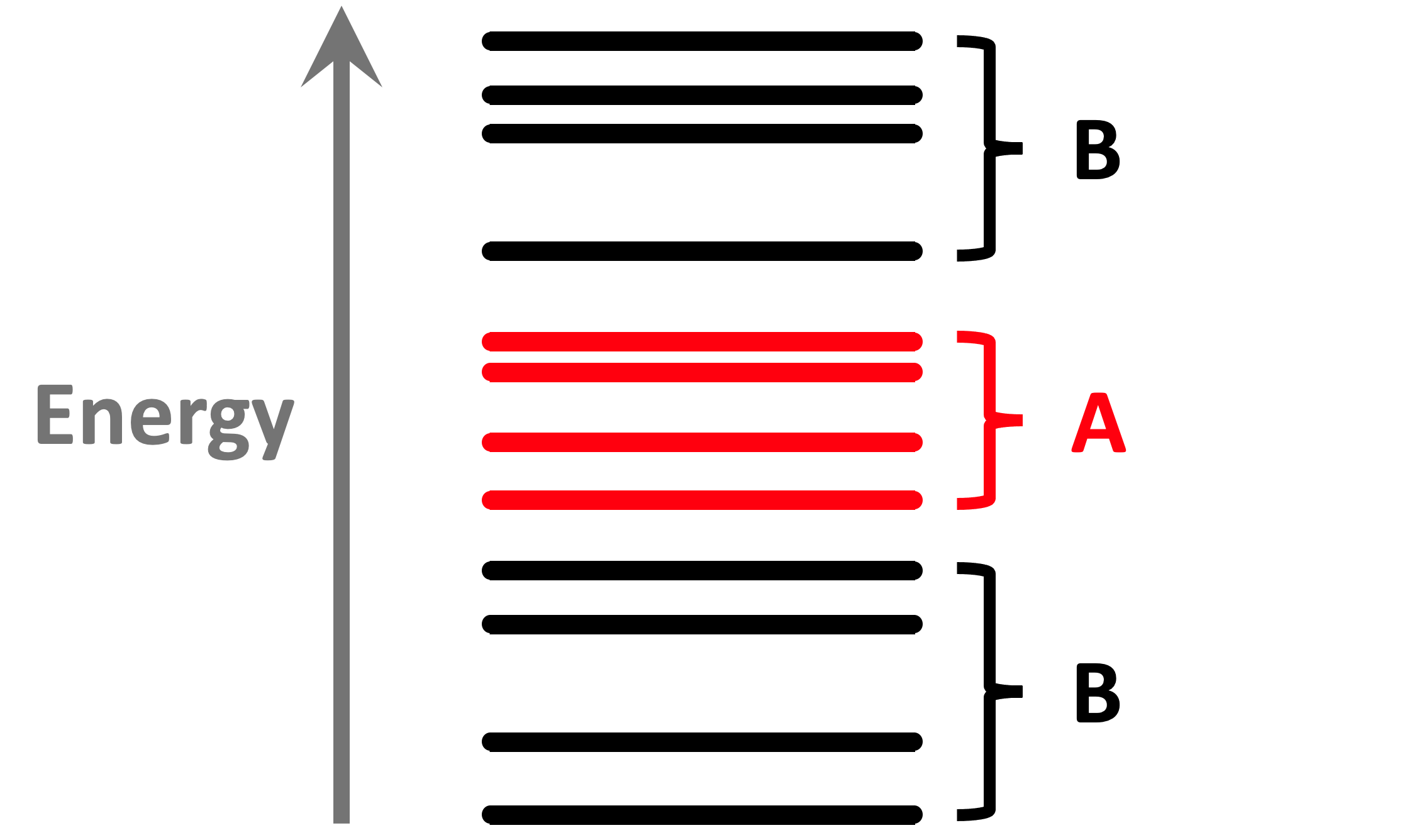
In practice, one is typically interested in groups of eigenstates, not in individual states. Let us denote the “active” group of interest by A and its complement by B, as depicted in Fig. 1. It is assumed that the A and B groups are well separated in energy, but degeneracies may be present within each of them. The completeness relation is

$${\mathbbm{1}}=\sum_{m}^{\rm A}\,|m\rangle\langle m|+\sum_{l}^{\rm B}\,|l\rangle\langle l|\equiv\sum_{j}^{\rm all}\,|j\rangle\langle j|\,.$$ (10)

In this paper we will consistently use indices $i,j,j^{\prime},\ldots$ to denote the whole set of Wannier states, while $m,n,n^{\prime},n^{\prime\prime},\ldots$ will denote states of subspace A, and $p,l,l^{\prime},l^{\prime\prime},\ldots$ for states in subspace B. We will assume that the repeated primed indices are summed (with the values running over the corresponding subspace), while the non-primed indices are not summed unless written explicitly (for the Trace quantities). Thus, from Sec. IV, we shorten the equation by omiting the $\sum$ symbols.

Let us start with the linear anomalous Hall conductivity given by second term in Eq. (3). To evaluate it we need the net Berry curvature $\Omega^{ab}_{\rm A}\equiv\sum_{n}^{\rm A}\,\Omega^{ab}$ of the occupied (A) states at each ${\bf k}$, where the Berry curvature of an individual state is $\Omega^{ab}_{n}=-2\mathrm{Im}\langle\kern-2.5pt\langle\partial_{a}n|\kern-1.5pt|\partial_{b}n\rangle\kern-2.5pt\rangle$ according to Eq. (6) (the index ${\bf k}$ has been omitted for brevity). Using the standard result from first-order non-degenerate perturbation theory, one obtains Xiao et al. (2010); Vanderbilt (2018)

$$|\partial_{a}n\rangle=-i\alpha_{n}|n\rangle+\sum_{j\not=n}\,|j\rangle\frac{\langle j|\partial_{a}{\cal H}|n\rangle}{\varepsilon_{n}-\varepsilon_{j}}$$ (11)

where $\alpha_{n}$ can be any real number. Inserting the completeness relation ${\mathbbm{1}}=\sum_{l}\,|j\rangle\langle j|$ The Berry curvature of a single band is

$$\Omega_{n}^{ab}=-2\mathrm{Im}\sum_{j\not=n}\,\frac{\langle n|\partial_{a}{\cal H}|j\rangle\langle j|\partial_{b}{\cal H}|n\rangle}{\left(\varepsilon_{n}-\varepsilon_{j}\right)^{2}}\,.$$ (12)

In typical applications one is more interested in the overall properties of groups of energy eigenstates than in the properties of individual eigenstates. For Eqs. (3-5), groups A and B comprise all states below and above the Fermi level at a given ${\bf k}$, respectively. For the linear anomalous Hall conductivity the net Berry curvature of the occupied states reads

$$\Omega_{\rm A}^{ab}=-2\mathrm{Im}\sum_{n}^{\rm A}\sum_{l}^{\rm B}\,\frac{\langle n|\partial_{a}{\cal H}|l\rangle\langle l|\partial_{b}{\cal H}|n\rangle}{\left(\varepsilon_{n}-\varepsilon_{l}\right)^{2}}\,.$$ (13)

where the double summation over states belonging to set A cancels out. Naturally, Eq. (13) reduces to Eq. (12) when group A contains a single state.

By virtue of having $(\varepsilon_{n}-\varepsilon_{l})^{2}$ in the denominator, Eq. (13) becomes resonantly enhanced in regions of the BZ where the gap between strongly-coupled A and B states is small. Conversely, the lack of energy denominators involving pairs of A states or pairs of B states means that $\Omega_{\rm A}^{ab}=-\Omega_{\rm B}^{ab}$ does not react strongly to band crossings and avoided crossings within each sector.

All of the above are familiar results. Consider now the gradient of the Berry curvature, which governs the quadratic anomalous Hall conductivity given by the second term in Eq. (4). Like $\Omega_{\rm A}^{ab}$ itself, $\partial_{c}\Omega_{\rm A}^{ab}$ should only react strongly to small energy gaps between the two groups A and B, not within each group. However, direct differentiation of Eq. (13) leads to an expression containing energy denominators between pairs of states within the same group. The problematic terms appear when differentiating the eigenstates using Eq. (11). If $n\in{\rm A}$, the summation over $j$ includes not only the B states but also the other A states, which can be arbitrarily close in energy to state $n$. Such unwanted terms cancel each other out in the final result for $\partial_{c}\Omega_{\rm A}^{ab}$, but making that cancelation explicit is not as straightforward as in the case of Eq. (13). For $\partial^{2}_{cd}\Omega_{\rm A}^{ab}$ and higher derivatives, achieving that cancellation becomes increasingly more difficult.

To circumvent the above problem, we will develop a systematic procedure for differentiating geometric quantities in such a way that the spurious terms are absent by construction. That procedure yields

$$\partial_{c}\Omega_{\rm A}^{ab}=-2\mathrm{Im}\sum_{n}^{\rm A}\sum_{l}^{\rm B}\,\frac{1}{\left(\varepsilon_{n}-\varepsilon_{l}\right)^{2}}\Bigg{\{}{\cal H}_{nl}^{,a}{\cal H}_{ln}^{,bc}+{\cal H}_{nl}^{,a}\Bigg{[}\sum_{n^{\prime}}^{\rm A}\,\frac{{\cal H}_{ln^{\prime}}^{,b}{\cal H}_{n^{\prime}n}^{,c}}{\varepsilon_{l}-\varepsilon_{n^{\prime}}}-\sum_{l^{\prime}}^{\rm B}\,\frac{{\cal H}_{ll^{\prime}}^{,b}{\cal H}_{l^{\prime}n}^{,c}}{\varepsilon_{l^{\prime}}-\varepsilon_{n}}+(b\leftrightarrow c)\Bigg{]}-(a\leftrightarrow b)\Bigg{\}}\,.$$ (14)

for the gradient of the Berry curvature of an effective-Hamiltonian model, where we have used a shortened notation ${\cal H}_{nl}^{,a}\equiv\langle n|\partial_{a}{\cal H}|l\rangle$ Like Eq. (13), Eq. (14) contains energy denominators between A and B states only, making it well-suited for numerical work. Interestingly, Equation (14) is symmetric under $b\leftrightarrow c$, which is connected to the known property of the berry curvature dipole Eqs. (7) and (77) to have zero trace. (see Appendix A for details)

In the following sections we will demonstrate how to systematically derive the derivatives of any order of Berry curvature, orbital magnetic moment, quantum metric and similar quantities, and at the end of Sec. V.3 the derivation of Eq. (14) will emerge.

III Non-Abelian covariant derivative

Table 1: Covariant derivative and its useful properties. $m,n,n^{\prime},n^{\prime\prime},\ldots\in A$, $p,l,l^{\prime},l^{\prime\prime},\ldots\in B$, summation over repeated primed indices is implied. See Sec. III for details.

Definition
$$X^{:d}_{nl}\equiv\partial_{d}X_{nl}+\,D^{d}_{nn^{\prime}}X_{n^{\prime}l}-\,X_{nl^{\prime}}D^{d}_{l^{\prime}l}$$ (15)
Matrix element of an operator $\hat{X}$
$\displaystyle X_{nl}^{:d}$ $\displaystyle=$ $\displaystyle X^{,d}_{nl}-D^{d}_{nl^{\prime}}X_{l^{\prime}l}+X_{nn^{\prime}}D^{d}_{n^{\prime}l}\,;$ (16a) $\displaystyle X_{ln}^{:d}$ $\displaystyle=$ $\displaystyle X^{,d}_{ln}-D^{d}_{ln^{\prime}}X_{n^{\prime}n}+X_{ll^{\prime}}D^{d}_{l^{\prime}n}\,;$ (16b) $\displaystyle X_{nm}^{:d}$ $\displaystyle=$ $\displaystyle X^{,d}_{nm}-D^{d}_{nl^{\prime}}X_{l^{\prime}m}+X_{nl^{\prime}}D^{d}_{l^{\prime}m}\,,$ (16c) $\displaystyle X^{,d}_{nl}$ $\displaystyle\equiv$ $\displaystyle\langle n|\partial_{d}\hat{X}|l\rangle$ (16d)
Hamiltonian ${\cal H}$
$${\cal H}_{nm}^{:d}={\cal H}_{nm}^{,d}\,,\quad{\cal H}_{nl}^{:d}=0$$ (17)
Trace Rule
$$\partial_{d}\left(X_{n^{\prime}n^{\prime}}\right)=X_{n^{\prime}n^{\prime}}^{:d}$$ (18)
Product Rule
$$\left(X_{rs^{\prime}}Y_{s^{\prime}t}\right)^{:d}=X_{rs^{\prime}}^{:d}Y_{s^{\prime}t}+X_{rs^{\prime}}Y_{s^{\prime}t}^{:d}$$ (19)
Chain Rule
$$\widetilde{f}_{ij}^{:d}={\cal H}^{:d}_{ij}\times\Biggl{\{}\begin{array}[]{lll}\left.\frac{df(\epsilon)}{d\epsilon}\right|_{\epsilon=\epsilon_{i}}&\mathrm{if}&\epsilon_{i}=\epsilon_{j}\\ \frac{f(\epsilon_{i})-f(\epsilon_{j})}{\epsilon_{i}-\epsilon_{j}}&\mathrm{if}&\epsilon_{i}\neq\epsilon_{j}\end{array}$$ (20)

Consider two isolated groups of bands $A$ and $B$, and a matrix $X_{nl}$ The only assumption is that $X_{nl}$ changes covariantly under gauge transformations $U_{A}$ and $U_{B}$ that act separately on the $A$ and $B$ band groups,

$$|n\rangle\overset{U^{A}}{\longrightarrow}\sum_{m}^{A}\,|m\rangle U^{A}_{mn}\,,\qquad|l\rangle\overset{U^{B}}{\longrightarrow}\sum_{p}^{B}\,|p\rangle U^{B}_{pl}\,.$$ (21)

That is, we assume that

$$X_{nl}\overset{U^{A}}{\longrightarrow}\sum_{m}^{A}\,\left(U^{A}\right)^{\dagger}_{nm}X_{ml}\,,\qquad X_{nl}\overset{U^{B}}{\longrightarrow}\sum_{p}^{B}\,X_{mp}U^{B}_{pl}\,.$$ (22)

The problem is that the simple derivative $X^{,d}_{nl}$ is not covariant in the above sense. This can be fixed by defining a “covariant derivative” as in Eq. (15) (see Tab. 1) Note that if $X$ is Hermitian or anti-Hermitian, then $X^{:d}$ has the same property. It can also be checked that if $X$ is covariant then $X^{:d}$ is also covariant.

If group $A$ contains a single band $n$ and group $B$ a single band $l$, we recover the Abelian definition of the covarant derivative given in Eq (9) of Ref. Aversa and Sipe (1995),

$$X^{;d}_{nl}=\partial_{d}X_{nl}-i\left(A^{d}_{nn}-A^{d}_{ll}\right)X_{nl}\,,$$ (23)

where we have written $D^{a}$ as $-iA^{a}$ for comparison purposes. To avoid confusion, we denote the non-Abelian covarant derivative by $X^{:d}$ and the Abelian one by $X^{;d}$.

Now let $\hat{X}$ be some operator. Then

$$X_{nl}^{:d} \equiv \langle n|\hat{X}|l\rangle^{:d}$$ (24)

$$= \langle n|\partial_{d}\hat{X}|l\rangle+\langle\partial_{d}n|\hat{X}|l\rangle+\langle n|\hat{X}|\partial_{d}l\rangle$$

$$+\sum_{n^{\prime\prime}}^{A}D^{d}_{nn^{\prime\prime}}X_{n^{\prime\prime}l}-\sum_{l^{\prime\prime}}^{B}X_{nl^{\prime\prime}}D^{d}_{l^{\prime\prime}l},$$

and inserting the a completeness relation (10) we get Eq. (16a) Hereinafter we will use a shortened notation (16d) If $n,l\in{\rm all}$ then only the first term survives, and our definition of the generalized derivative reduces to Eq. (34) of Ref. Ventura et al. (2017). Eq. (16a) shows off-diagonal “AB” blocks of the matrix. The diagonal block (“AA”) can be derived in a similar way to get Eq. (16c) and the “BA” and “BB” parts may be obtained by interchanging A and B in equations above. One special case is the Hamiltonian operator $\hat{\cal H}$, which is represented by a diagonal matrix. Using ${\cal H}_{nl}=0$ and ${\cal H}^{,d}_{nl}=D^{d}_{nl}(\varepsilon_{l}-\varepsilon_{n})$ we find the simple results given by Eq. (17). Thus we see, that although Hamiltonian is a diagonal matrix, its covariant derivative is only block-diagonal.

It is important to show some useful properties of the covariant derivative, summarized in Tab. 1.

Trace rule. First of all, in applications we will be interested in taking derivatives of a trace of matrix over subspace A. Using Eq. (15), that can be written as

$$\partial_{d}\sum_{n}X_{nn}=\sum_{n}\partial_{d}X_{nn}=\\ \sum_{n}X^{:d}_{nn}+\sum_{nn^{\prime}}^{A}\,D^{d}_{nn^{\prime}}X_{n^{\prime}n}-\sum_{nn^{\prime}}^{A}\,X_{nn^{\prime}}D^{d}_{n^{\prime}n}$$ (25)

and noting that the last to term are the same, upto the sign and interchange of indices $n\leftrightarrow n^{\prime}$, we arrive at Eq. (18)

Product rule. Consider two covariant matrices $X_{rs}$ and $Y_{st}$ matrices with $r\in C_{1}$, $s\in C_{2}$ and $t\in C_{3}$ (where each subspace $C_{i}$ may independently be equal to A or B). Taking the covariant derivative of their product explicitly we get

$$\left(\sum_{s}^{C_{2}}X_{rs}Y_{st}\right)^{:d}=\sum_{s}^{C_{2}}\Bigl{(}\left(\partial_{d}X_{rs}\right)Y_{st}+X_{rs}\partial_{d}\left(Y_{st}\right)\\ +\sum_{r^{\prime}}^{C_{1}}D^{d}_{rr^{\prime}}X_{r^{\prime}s}Y_{st}-\sum_{t^{\prime}}^{C_{3}}X_{rs}Y_{st^{\prime}}D_{t^{\prime}t}^{d}\Bigr{)}$$ (26)

Now, adding and subtracting $\sum_{ss^{\prime}}^{C_{2}}X_{rs}D_{ss^{\prime}}^{d}Y_{s^{\prime}t}$ we arrive at Eq. (19), which is similar to the product rule for the simple derivatives.

Chain rule. In some cases equations may contain a scalar-valued smooth function of the electron energies $f(\epsilon_{i})$. Taking the covariant derivatives of such functions is less intuitive than the product and trace rule. To do it correctly, we represent $f$ as a gauge-covariant matrix,

$$\widetilde{f}_{ij}=\delta_{ij}f(\epsilon_{i})$$ (27)

This matrix is diagonal, however, its covariant derivative does not have to be diagonal (as we saw for the Hamiltonian in Eq. (17). Employing a Taylor expansion and a product rule we arrive at Eq. (20), as shown in in Appendix Appendix B.

IV Catalogue of geometric quantities

Before proceeding with derivation of explicit equations for Wannier interpolation of multiple geometrical quantities of interest, we first define them in a gauge-covariant way and show that they all may be reduced to two objects $\widetilde{F}^{ab}_{mn}$ and $\widetilde{H}^{ab}_{mn}$ defined below.

IV.1 Gauge-covariant matrices

Let $P=\sum_{n}^{\rm A}\,|u_{n}\rangle\langle u_{n}|$ and $Q=1-P$. The states $|u_{n}\rangle$ within the active space A are not assumed to be energy eigenstates, so that in general the Hamiltonian matrix

$${\cal H}_{mn}\equiv\langle u_{m}|\hat{\cal H}|u_{n}\rangle$$ (28)

is not diagonal. Following Eqs. (6-8) of Ref. Lopez et al. (2012) We write the three gage-covariant quantities

$$\widetilde{F}^{ab}_{mn} \equiv\langle u_{m}|(\partial_{a}P)Q(\partial_{b}P)|u_{n}\rangle=\langle\partial_{a}u_{m}|Q|\partial_{b}u_{n}\rangle\,,$$ (29)

$$\widetilde{G}^{ab}_{mn} \equiv\frac{1}{2}\langle u_{m}|{\cal H}(\partial_{a}P)Q(\partial_{b}P)+(\partial_{a}P)Q(\partial_{b}P){\cal H}|u_{n}\rangle=$$

$$=\frac{1}{2}\left({\cal H}_{mn^{\prime}}\widetilde{F}^{ab}_{n^{\prime}m}+\widetilde{F}^{ab}_{mn^{\prime}}{\cal H}_{n^{\prime}n}\right)\,,$$ (30)

$$\widetilde{H}^{ab}_{mn} \equiv\langle u_{m}|(\partial_{a}P)Q{\cal H}Q(\partial_{b}P)|u_{n}\rangle=\langle\partial_{a}u_{m}|Q{\cal H}Q|\partial_{b}u_{n}\rangle\,,$$ (31)

and also

$$\widetilde{S}^{ab}_{mn}\equiv\frac{\hbar^{2}}{m_{e}}\delta_{ab}\delta_{mn}+2\left(\widetilde{G}^{ab}_{mn}-\widetilde{H}^{ab}_{mn}\right)\,.$$ (32)

The four matrices $\widetilde{O}^{ab}_{mn}$ with $O=F,G,H,S$ are Hermitian in the sence that $\widetilde{O}^{ab}_{mn}=\left(\widetilde{O}^{ba}_{nm}\right)^{*}$, and they (as well as ${\cal H}_{mn}$) transform covariantly under unitary gauge transformations of the form $|u_{n}\rangle\rightarrow|u^{\prime}_{n}\rangle=\sum_{m}^{\rm A}|u_{m}\rangle U_{mn}$, that is, $\widetilde{O}^{ab}\rightarrow U^{\dagger}\widetilde{O}^{ab}U$.

$\widetilde{F}^{ab}_{mn}$ is the metric-curvature tensor, from which the covariant quantum metric and Berry curvature tensors can be obtained as

$$\widetilde{\mathfrak{F}}^{ab}_{mn}\equiv\frac{1}{2}\widetilde{F}^{ab}_{mn}+\frac{1}{2}\widetilde{F}^{ba}_{mn}$$ (33)

and

$$\widetilde{\Omega}^{c}_{mn}\equiv i\epsilon_{abc}\widetilde{F}^{ab}_{mn}\,,$$ (34)

respectively. In the same way, we can extract from $\widetilde{S}^{ab}_{mn}$ two new covariant tensors

$$\widetilde{\mathfrak{S}}^{ab}_{mn}\equiv\frac{1}{2}\widetilde{S}^{ab}_{mn}+\frac{1}{2}\widetilde{S}^{ba}_{mn}$$ (35)

and

$$\widetilde{\cal S}^{c}_{mn}\equiv i\epsilon_{abc}\widetilde{S}^{ab}_{mn}\,.$$ (36)

$\widetilde{\mathfrak{S}}^{ab}_{mn}$ is a generalized inverse effective mass tensor in a sense to be clarified shortly, and $\widetilde{\cal S}^{c}_{mn}$ is a generalized orbital magnetic moment tensor in the following sense: if the A states are all degenerate with energy $\varepsilon_{\rm A}$, so that ${\cal H}_{mn}=\varepsilon_{\rm A}\delta_{mn}$ in any gauge, the matrices $\widetilde{m}^{c}_{mn}=(e/4\hbar)\widetilde{\cal S}^{c}_{mn}$ and $\widetilde{L}^{c}_{mn}=-(m_{e}/2\hbar)\widetilde{\cal S}^{c}_{mn}$ reduce to the orbital moment and orbital angular momentum matrices as defined in Eq. (51) of Ref. Chang and Niu (2008),

$$\frac{2\hbar}{e}\widetilde{m}^{c}_{mn}=-\frac{\hbar}{m_{e}}\widetilde{L}^{c}_{mn}=i\epsilon_{abc}\left(\varepsilon_{\rm A}\widetilde{F}^{ab}_{mn}-\widetilde{H}^{ab}_{mn}\right)=\\ =i\epsilon_{abc}\langle\partial_{a}u_{m}|Q(\varepsilon_{\rm A}-{\cal H})Q|\partial_{b}u_{n}\rangle\,.$$ (37)

Finally, we also introduce a ${\bf k}$-resolved orbital magnetization matrix

$$\frac{2\hbar}{e}\widetilde{M}^{c}_{mn}\equiv-i\epsilon_{abc}\left(\widetilde{H}^{ab}_{mn}+\widetilde{G}^{ab}_{mn}-2\epsilon_{\rm F}\widetilde{F}^{ab}_{mn}\right)=$$ (38)

$$=\frac{2\hbar}{e}\widetilde{m}^{c}_{mn}+2i\epsilon_{abc}\left(\epsilon_{\rm F}\widetilde{F}^{ab}_{mn}-\widetilde{G}^{ab}_{mn}\right)\,.$$ (39)

IV.2 Gauge-invariant traces

Given a covariant matrix $\widetilde{O}_{mn}$ with $m,n\in{\rm A}$, we write its (gauge-invariant) trace as

$$O_{\rm A}\equiv\mathrm{Tr}_{\rm A}\,\widetilde{O}=\sum_{n}^{\rm A}\,\widetilde{O}_{nn}\,.$$ (40)

Thus ${\mathfrak{F}}^{ab}_{\rm A}={\mathfrak{F}}^{ba}_{\rm A}$ and ${\Omega}^{c}_{\rm A}$ are the net quantum metric and Berry curvature of the A states respectively, $M^{c}_{\rm A}$ is their net ${\bf k}$-resolved orbital magnetization, and ${\mathfrak{S}}^{ab}_{\rm A}={\mathfrak{S}}^{ba}_{\rm A}$ is the sum of the inverse effective masses (times $\hbar^{2}$) of the A band states,

$${\mathfrak{S}}^{ab}_{\rm A}:=\sum_{n}^{\rm A}\,\partial^{2}_{ab}\varepsilon_{n}\,.$$ (41)

Here the symbol $:=$ denotes an equality whose right-hand-side only holds in a gauge where the Hamiltonian matrix is diagonal: ${\cal H}_{mn}=\varepsilon_{m}\delta_{mn}$.

If space A contains a single band $n$, we simplify the notation as $\widetilde{O}^{ab}_{mn}\rightarrow O^{ab}_{n}$. In that limit Eqs. (29-31) reduce to

$$F^{ab}_{n} =\langle\partial_{a}u_{n}|\partial_{b}u_{n}\rangle-\langle\partial_{a}u_{n}|u_{n}\rangle\langle u_{n}|\partial_{b}u_{n}\rangle\,,$$ (42)

$$G^{ab}_{n} =\varepsilon_{n}F^{ab}_{n}\,,$$ (43)

$$H^{ab}_{n} =\langle\partial_{a}u_{n}|{\cal H}|\partial_{b}u_{n}\rangle-\varepsilon_{n}\langle\partial_{a}u_{n}|u_{n}\rangle\langle u_{n}|\partial_{b}u_{n}\rangle\,,$$ (44)

and Eq. (32) becomes

$$S^{ab}_{n}=\frac{\hbar^{2}}{m_{e}}\delta_{ab}+2\langle\partial_{a}u_{n}|(\varepsilon_{n}-{\cal H})|\partial_{b}u_{n}\rangle\,,$$ (45)

which agrees with the expression given in Ref. Gao et al. (2015) (see the 2nd column of p. 3 therein).

In the same limit Eqs. (33) and (34) reduce to the single-band quantum metric and Berry curvature, respectively,

$${\mathfrak{F}}^{ab}_{n} =\mathrm{Re}\,F^{ab}_{n}=\mathrm{Re}\langle\partial_{a}u_{n}|\partial_{b}u_{n}\rangle-\langle\partial_{a}u_{n}|u_{n}\rangle\langle\partial_{b}u_{n}|u_{n}\rangle\,,$$ (46)

$${\Omega}^{c}_{n} =-\epsilon_{abc}\mathrm{Im}\,F^{ab}_{n}=-\mathrm{Im}\,\langle\nabla_{\bf k}u_{n}|\times|\nabla_{\bf k}u_{n}\rangle_{c}\,,$$ (47)

Eqs. (35) and (36) become proportional to the single-band inverse effective mass and orbital moment, respectively,

$${\mathfrak{S}}^{ab}_{n}=\mathrm{Re}\,S^{ab}_{n}=\\ =\frac{\hbar^{2}}{m_{e}}\delta_{ab}+2\mathrm{Re}\langle\partial_{a}u_{n}|(\varepsilon_{n}-{\cal H})|\partial_{b}u_{n}\rangle=\partial^{2}_{ab}\varepsilon_{n}\,,$$ (48)

$${\cal S}^{c}_{n}=-\epsilon_{abc}\mathrm{Im}\,S^{ab}_{n}=\\ =-2\mathrm{Im}\langle\nabla_{\bf k}u_{n}|\times(\varepsilon_{n}-{\cal H})|\nabla_{\bf k}u_{n}\rangle_{c}=\frac{4\hbar}{e}m^{c}_{n}\,,$$ (49)

and Eq. (39) becomes the single-band ${\bf k}$-resolved orbital magnetization,

$$\frac{2\hbar}{e}M^{c}_{n}=\mathrm{Im}\langle\nabla_{\bf k}|\times\left({\cal H}+\varepsilon_{n}-2\varepsilon_{\rm F}\right)|\nabla_{\bf k}u_{n}\rangle_{c}\,,$$ (50)

or equivalently,

$$M^{c}_{n}=m^{c}_{n}+\frac{e}{\hbar}(\varepsilon_{\rm F}-\varepsilon_{n}){\Omega}^{c}_{n}\,.$$ (51)

Suppose that space A is entirely made up of bands that never touch one another. Then its net Berry curvature, inverse effective mass, and orbital magnetization are equal to the sums over bands of the corresponding single-band quantities,

$${\Omega}^{c}_{\rm A}=\sum_{n}^{\rm A}\,\Omega^{c}_{n}\,,\quad{\mathfrak{S}}^{ab}_{\rm A}=\sum_{n}^{\rm A}\,{\mathfrak{S}}^{ab}_{n}\,,\quad M^{c}_{\rm A}=\sum_{n}^{\rm A}\,M^{c}_{n}\,,$$ (52)

and such quantities are said to be “band additive.” Note that the quantum metric and the orbital moment are not band additive, since in general

$${\mathfrak{F}}^{ab}_{\rm A}\not=\sum_{n}^{\rm A}\,{\mathfrak{F}}^{ab}_{n}\,,\quad{\cal S}^{c}_{\rm A}\not=\sum_{n}^{\rm A}\,{\cal S}^{c}_{n}\,.$$ (53)

V Wannier interpolation

V.1 Wannier functions and effective models

In this section we introduce the necessary notation, and briefly recall the spirint of Wannier interpolation of Berry curvature, closely following Ref. Wang et al. (2006).

Wannier functions $|{\bf R}j\rangle$ form a localized orthonormal basis for the description of electron bandstructure.Marzari et al. (2012) The eigenvalues of the Wannier Hamiltonian

$${\cal H}^{\text{W}}_{ij}({\bf k})=\sum_{\bf R}\,e^{i{\bf k}\cdot({\bf R}+{\bf t}_{j}-{\bf t}_{i})}{\cal H}^{\text{W}}_{ij}({\bf R})\,.$$ (54)

accurately reproduce the eigenvalues of the Bloch bands computed from first principles. Here ${\bf R}$ are lattice vectors, and the matrix elements ${\cal H}^{\text{W}}_{ij}({\bf R})$ are computed as

$${\cal H}^{\text{W}}_{ij}({\bf R})=\langle{\bf R}^{\prime}i|\hat{{\cal H}}|{\bf R}^{\prime}+{\bf R},j\rangle=\langle{\bf 0}i|\hat{\cal H}|{\bf R}j\rangle\,,$$ (55)

and the orthonormality condition reads

$$\langle{\bf R}^{\prime}i|{\bf R}j\rangle=\delta_{{\bf R}{\bf R}^{\prime}}\delta_{ij}$$ (56)

The electron energies and wavefunctions at any arbitrary wavevector ${\bf k}$ are obtained from the secular equation

$${\cal H}^{\text{W}}({\bf k})U_{{\bf k}n}=\varepsilon_{{\bf k}n}U_{{\bf k}n}\,,$$ (57)

to find the eigenenergies $\varepsilon_{{\bf k}n}$ and column vectors $|n\rangle$ of coefficients $U_{jn}({\bf k})$ of the expansion of the wavefunctions

$$|u_{j{\bf k}}\rangle=|u^{\text{W}}_{j^{\prime}{\bf k}}\rangle U_{j^{\prime}j}({\bf k})$$ (58)

in the Bloch basis $|u^{\text{W}}_{j{\bf k}}\rangle$ constructed from Wannier functions as

$$|u^{\text{W}}_{j{\bf k}}\rangle=\sum_{\bf R}e^{i{\bf k}\cdot({\bf R}+{\bf t}_{j}-{\bf r})}|{\bf R}j\rangle\,.$$ (59)

We have included Wannier centers ${\bf t}_{i}$ in the phase factors the phase factor, as this is the most convenient convention for handling Berry-phase quantities Vanderbilt (2018).(See Appendix E for details )

The derivative of states $|n\rangle$ of the Wannier Hamiltonian is given by Eq. (11) the and taking inner product with $\langle l|$ yields the anti-Hermitian matrix

$$D^{a}_{ln}=\langle l|\partial_{a}n\rangle=\begin{cases}\displaystyle\frac{\langle\kern-2.5pt\langle l|\kern-1.5pt|\partial_{a}{\cal H}^{\text{W}}|\kern-1.5pt|n\rangle\kern-2.5pt\rangle}{\varepsilon_{n}-\varepsilon_{l}},&\text{if $l\not=n$}\\ -i\alpha_{n},&\text{if $l=n$}\end{cases}\,.$$ (60)

which is convenient for the evaluation of the derivative of Bloch states as

$$|\partial_{b}u_{n}\rangle=|\partial_{b}u_{j^{\prime}}^{\text{W}}\rangle U_{j^{\prime}n}+|u_{j^{\prime}}\rangle D_{{j^{\prime}}n}^{b}$$ (61)

Inserting Eq. (61) into Eq. (6) and summing over states in set A one gets the net Berry curvature

$$\Omega^{ab}_{\mathrm{A}} = \Omega^{ab}_{\mathrm{A,int}}+\Omega^{ab}_{\mathrm{A,ext}}~{};$$ (62a)

$$\Omega^{ab}_{\mathrm{A,int}} = 2\mathrm{Im}\sum^{A}_{n}\sum^{B}_{l}D^{a}_{nl}D^{b}_{ln}~{};$$ (62b)

$$\Omega^{ab}_{\mathrm{A,ext}} = -2\mathrm{Im}\sum^{A}_{n}\overline{F}^{ab}_{nn}-4\mathrm{Re}\sum^{A}_{n}\sum^{B}_{l}D^{a}_{nl}\overline{A}^{b}_{ln}~{},$$ (62c)

which we have separated into “internal” and “external” terms for a reason that will be explained shortly. Hereinafter, with an overline we denote a transform of any matrix object in the Wannier gauge ${\cal O}^{\text{W}}_{\bf k}$ into to the Hamiltonian gauge:

$$\overline{\cal O}_{mn}=\langle m|{\cal O}^{\text{W}}_{\bf k}|n\rangle=\left(U^{\dagger}\cdot{\cal O}\cdot U\right)_{mn}$$ (63)

and the corresponding Wannier gauge matrices $A^{\text{W}}$ and $F^{\text{W}}$ are defined in Eqs. (92a) and (92d) based on the real-space matrix elements (93).

In the derivations above, one could replace the Wannier functions to any other set of orthonormal localized basis states $|{\bf R}j\rangle$. In fact, the derivation would be the same for an empirical tight-binding model, with the only difference that the matrix elements ${\cal H}_{ij}({\bf R})$, $\mathbb{A}^{a}_{ij}({\bf R})$ and $\mathbb{F}^{a}_{ij}({\bf R})$ would not be computed via Eqs. (55) and (93), but rather fitted to bandstructure or chosen empirically. It is a common practice in tight-binding models to neglect matrix elements (93), and work only with the “hoppings” ${\cal H}({\bf R})$. Also, when working with an effective ${\bf k}\cdot\mathbf{p}$ model, there are no localized functions, but instead the Hamiltonian matrix is assumed to be written in a basis that does not depend on ${\bf k}$, and therefore the first term in Eq. (61) vanishes. In these cases the Berry curvature is given only by $\Omega^{ab}_{\mathrm{A,int}}$ which is identical to Eq. (13). The terms that survive in the case of an effective model are called internal because they are the property of a Hamiltonian. In turn, the terms that depend on additional matrix elements are called external, and they are important for an accurate ab initio description of electronic properties. In the rest of the present article we will keep this separation.

V.2 Wannier interpolation of $\widetilde{F}^{ab}_{mn}$ and $\widetilde{H}^{ab}_{mn}$

In this section we derive the Wannier interpolation of quantities given by Eqs. (29) and (31). Recalling that $Q=1-|u_{n^{\prime}}\rangle\langle u_{n^{\prime}}|$ from Eq. (61) we obtain

$$Q|\partial_{b}u_{n}\rangle=Q|\partial_{b}u_{j^{\prime}}^{\text{W}}\rangle U_{{j^{\prime}}n}+|u_{l^{\prime}}\rangle D_{l^{\prime}n}^{b}=\\ |\partial_{b}u_{j^{\prime}}^{\text{W}}\rangle U_{j^{\prime}n}-|u_{n^{\prime}}\rangle\langle u_{n^{\prime}}|\partial_{b}u_{j^{\prime}}^{\text{W}}\rangle U_{j^{\prime}n}+|u_{l^{\prime}}\rangle D_{l^{\prime}n}^{b}=\\ |\partial_{b}u_{j^{\prime}}^{\text{W}}\rangle U_{j^{\prime}n}+i\sum_{n^{\prime}}^{A}|u_{n^{\prime}}\rangle\overline{A}^{b}_{n^{\prime}n}+|u_{l^{\prime}}\rangle D_{l^{\prime}n}^{b}$$ (64)

and using and $Q^{2}=Q$ we obtain the following expressions:

$$\widetilde{F}^{ab}_{mn} = \widetilde{F}^{ab}_{mn,\textrm{int}}+\widetilde{F}^{ab}_{mn,\textrm{ext}}$$ (65a)

$$\widetilde{F}^{ab}_{mn,\textrm{int}} = -D_{nl^{\prime}}^{a}D_{l^{\prime}m}^{b}$$ (65b)

$$\widetilde{F}^{ab}_{mn,\textrm{ext}} = \left[\left(iD^{a}_{nl^{\prime}}\overline{A}^{b}_{l^{\prime}m}\right)+\left({}_{m\leftrightarrow n}^{a\leftrightarrow b}\right)^{*}\right]$$ (65c)

$$+\overline{F}^{ab}_{mn}-\overline{A}^{a}_{mn^{\prime}}\overline{A}^{b}_{n^{\prime}n}$$

and

$$\widetilde{H}^{ab}_{mn} = \widetilde{H}^{ab}_{mn,\textrm{int}}+\widetilde{H}^{ab}_{mn,\textrm{ext}}$$ (66a)

$$\widetilde{H}^{ab}_{mn,\textrm{int}} = -D_{nl^{\prime}}^{a}{\cal H}_{l^{\prime}l^{\prime\prime}}D_{l^{\prime\prime}m}^{b}$$ (66b)

$$\widetilde{H}^{ab}_{mn,\textrm{ext}} = \left[\left(iD^{a}_{nl^{\prime}}\overline{B}^{b}_{l^{\prime}m}\right)+\left({}_{m\leftrightarrow n}^{a\leftrightarrow b}\right)^{*}\right]+$$ (66c)

$$+\overline{H}^{ab}_{mn}-\overline{A}^{a}_{mm^{\prime}}{\cal H}_{m^{\prime}n^{\prime}}\overline{A}^{b}_{n^{\prime}n}$$

Similar to Eq. (62) we have separated the result into internal and external terms. Here the bar above a matrix follows Eq. (63). To describe the external terms, And following Wang et al. (2006) and Lopez et al. (2012) we have defined a series of quantities defined in the Wannier gauge:

$$\left(A^{\text{W}}\right)^{a}_{ij} \equiv i\langle u_{i}^{\text{W}}|\partial_{a}u_{j}^{\text{W}}\rangle$$ (67a)

$$\left(B^{\text{W}}\right)^{a}_{ij} \equiv i\langle u_{i}^{\text{W}}|{\cal H}|\partial_{a}u_{j}^{\text{W}}\rangle$$ (67b)

$$\left(H^{\text{W}}\right)^{ab}_{ij} \equiv \langle\partial_{a}u_{i}^{\text{W}}|{\cal H}|\partial_{b}u_{j}^{\text{W}}\rangle$$ (67c)

$$\left(F^{\text{W}}\right)^{ab}_{ij} \equiv \langle\partial_{a}u_{i}^{\text{W}}|\partial_{b}u_{j}^{\text{W}}\rangle$$ (67d)

Evaluation of these quantities is given in Appendix D

Inserting Equations (65) and (66) into corresponding equations from Sec. IV one can obtain Wannier interpolation of the needed geometrical quantity. For instance, combining (65), (34) and (40) one obtains the known result for Berry curvature (62).

V.3 Covariant derivatives of $\widetilde{F}^{ab}_{mn}$ and $\widetilde{H}^{ab}_{mn}$

Now we are ready to take the covariant derivatives of Eqs. (65a) and (66c), using the product rule defined in Eq. (19).

$$\widetilde{F}^{ab:d}_{mn} = \widetilde{F}^{ab:d}_{mn,\textrm{int}}+\widetilde{F}^{ab:d}_{mn,\textrm{ext}}$$ (68a)

$$\widetilde{F}^{ab:d}_{mn,\textrm{int}} = D_{ml^{\prime}}^{a}D_{l^{\prime}n}^{b:d}+\left({}_{m\leftrightarrow n}^{a\leftrightarrow b}\right)^{*}$$ (68b)

$$\widetilde{F}^{ab:d}_{mn,\textrm{ext}} = -\Bigl{[}\Bigl{(}i\overline{A}^{a}_{ml^{\prime}}D^{b:d}_{l^{\prime}n}+iD^{a}_{ml^{\prime}}\overline{A}^{b:d}_{l^{\prime}n}$$ (68c)

$$+\overline{A}_{mn^{\prime}}^{a}\overline{A}_{n^{\prime}n}^{b:d}\Bigr{)}+\left({}_{m\leftrightarrow n}^{a\leftrightarrow b}\right)^{*}\Bigr{]}+\overline{F}^{ab:d}_{mn}$$

$$\widetilde{H}^{ab:d}_{mn} = \widetilde{H}^{ab:d}_{mn,\textrm{int}}+\widetilde{H}^{ab:d}_{mn,\textrm{ext}}$$ (69a)

$$\widetilde{H}^{ab:d}_{mn,\textrm{int}} = -\Bigl{[}D_{ml^{\prime}}^{a}{{\cal H}_{l^{\prime}l^{\prime\prime}}}D_{l^{\prime\prime}n}^{b:d}+\left({}_{m\leftrightarrow n}^{a\leftrightarrow b}\right)^{*}\Bigr{]}$$ (69b)

$$-D_{ml^{\prime}}^{a}{\cal H}_{l^{\prime}l^{\prime\prime}}^{,d}D_{l^{\prime\prime}n}^{b}$$

$$\widetilde{H}^{ab:d}_{mn,\textrm{ext}} = \Bigl{[}i(\overline{B}^{\dagger})^{a}_{ml^{\prime}}D^{b:d}_{l^{\prime}n}+iD^{a}_{ml^{\prime}}\overline{B}^{b:d}_{l^{\prime}n}$$ (69c)

$$-\overline{A}_{mm^{\prime}}^{a}{\cal H}_{m^{\prime}n^{\prime}}\overline{A}_{n^{\prime}n}^{b:d}+\left({}_{m\leftrightarrow n}^{a\leftrightarrow b}\right)^{*}\Bigr{]}-$$

$$-\overline{A}_{mm^{\prime}}^{a}{\cal H}_{m^{\prime}n^{\prime}}^{,d}\overline{A}_{n^{\prime}n}^{b}+\overline{H}^{ab:d}_{mn}$$

Now we need to find the generalized derivatives of the ingredients of this equation.

The derivatives $\overline{A}^{b:d}_{ln}$, $\overline{B}^{b:d}_{ln}$, $\overline{C}^{b:d}_{ln}$ and $\overline{F}^{b:d}_{ln}$ are evaluated in a general way. Consider a quantity of the form of Eq. (63), Eq. (16c) for instance reads

$$\overline{\cal O}^{:d}_{nn^{\prime}}=\overline{\cal O}^{,d}_{nn^{\prime}}-\sum_{l}^{B}D^{d}_{nl}{\cal O}_{ln^{\prime}}+\sum_{l}^{B}{\cal O}_{nl}D^{d}_{ln^{\prime}}$$ (70)

where in accordance with Eq. (16d) we defined

$$\overline{\cal O}^{,d}\equiv\overline{\partial_{d}{\cal O}}=U^{\dagger}\left(\partial_{d}{\cal O}^{\text{W}}\right)U\,.$$ (71)

Some technical notes on the evaluation on the evaluation of $\overline{B}^{b:d}_{ln}$ are left for Appendix LABEL:sec:B-frozen. In order to derive $D_{ln}^{b:d}$ let’s rewrite Eq. (60) for $D^{b}_{ln}$ as

$$D_{ln^{\prime}}^{b}{\cal H}_{n^{\prime}n}-{\cal H}_{ll^{\prime}}D_{l^{\prime}n}^{b}={\cal H}_{ln}^{,b}~{}.$$ (72)

Now we take the covariant derivative of both sides of this equation and employing the product rule Eq. (19) we get

$$D_{ln^{\prime}}^{b}{\cal H}_{n^{\prime}n}^{:d}+D_{ln^{\prime}}^{b:d}{\cal H}_{n^{\prime}n}-{\cal H}_{ll^{\prime}}D_{l^{\prime}n}^{b:d}-{\cal H}_{ll^{\prime}}^{:d}D_{l^{\prime}n}^{b}=\\ {\cal H}_{ln}^{,bd}-D_{ln^{\prime}}^{d}{\cal H}_{n^{\prime}n}^{,b}+{\cal H}_{ll^{\prime}}^{,b}D_{l^{\prime}n}^{d}$$ (73)

where we also used Eq. (16b) for ${\cal H}_{ln}^{,b:d}$ and Eq. (17)

Now, consider this equation in the Hamiltonian gauge, collect all terms except $D_{nl^{\prime}}^{b:d}$ in the RHS and divide by $(\varepsilon_{n}-\varepsilon_{l})\equiv\varepsilon_{nl}$ to get the following expression

$$D^{b:d}_{ln}=\frac{1}{\varepsilon_{nl}}\left[{\cal H}^{,bd}_{ln}+\left({\cal H}^{,b}_{ll^{\prime}}D^{d}_{l^{\prime}n}-D^{d}_{ln^{\prime}}{\cal H}^{,b}_{n^{\prime}n}+(b\leftrightarrow d)\right)\right]$$ (74)

It can be seen that the derived equations do not contain the $D$ matrix states A, as well as between states B. As far as spaces A and B are By construction, this behaviour will be preserved in evaluation of higher derivatives (see Appendix F).

Inserting Equations (68a) and (69a) into corresponding equations from Sec. IV one can obtain Wannier interpolation of thederivatives of the needed geometrical quantities. For instance, combining (68b), (18), (34) and (74) one obtains the known result for derivative of the Berry curvature of occupied states (14), that we gave in Sec. II without proof.

VI First principles results: trigonal Tellurium

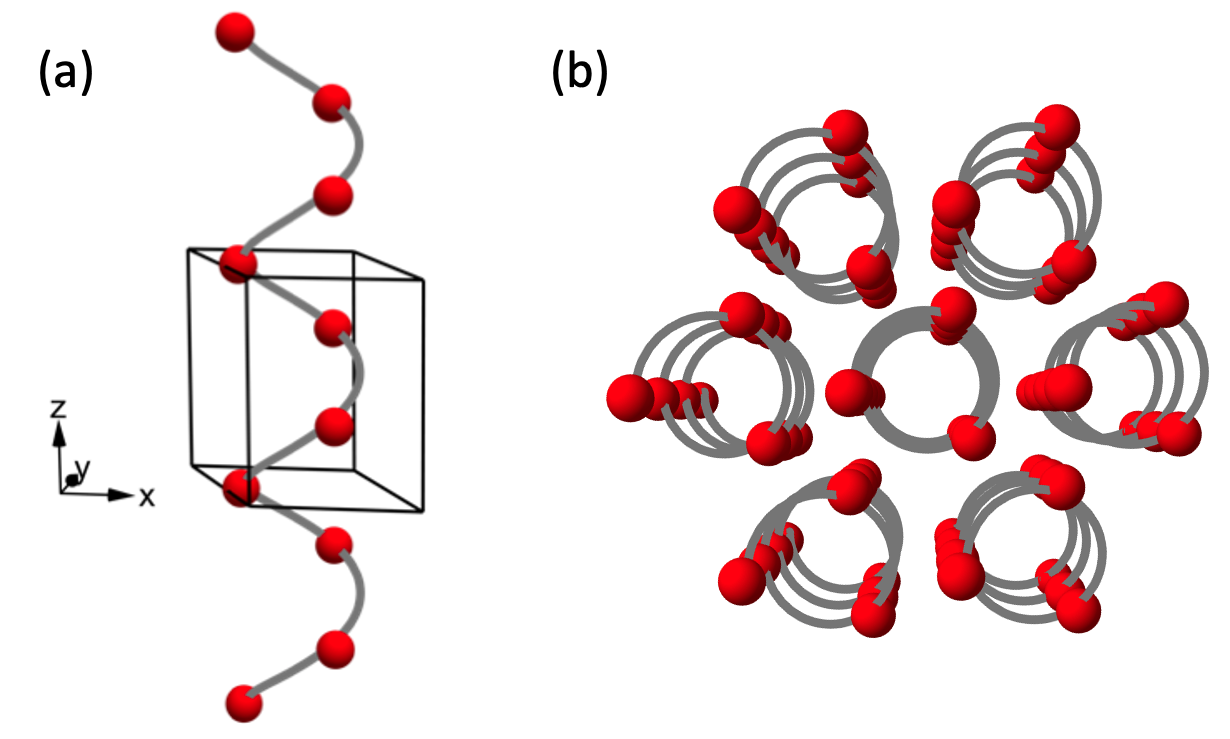
Trigonal Tellurium has a crystal structure composed of homotropic triple helix Te-chains with space group $P3_{1}21$ (right handed) or $P3_{2}21$ (left handed), the right handed structure of Te is shown in Fig. 2. The three Te atoms in each unit cell are evenly distributed along the helix. The screw structure breaks inversion symmetry and creates a Berry curvature dipole.

Figure 2: Crystal structure of tellurium with space group $P3_{1}21$.(a) The tellurium chains spiral along z-axes of the crystal lattice. (b) Top view of Te spiral chains.

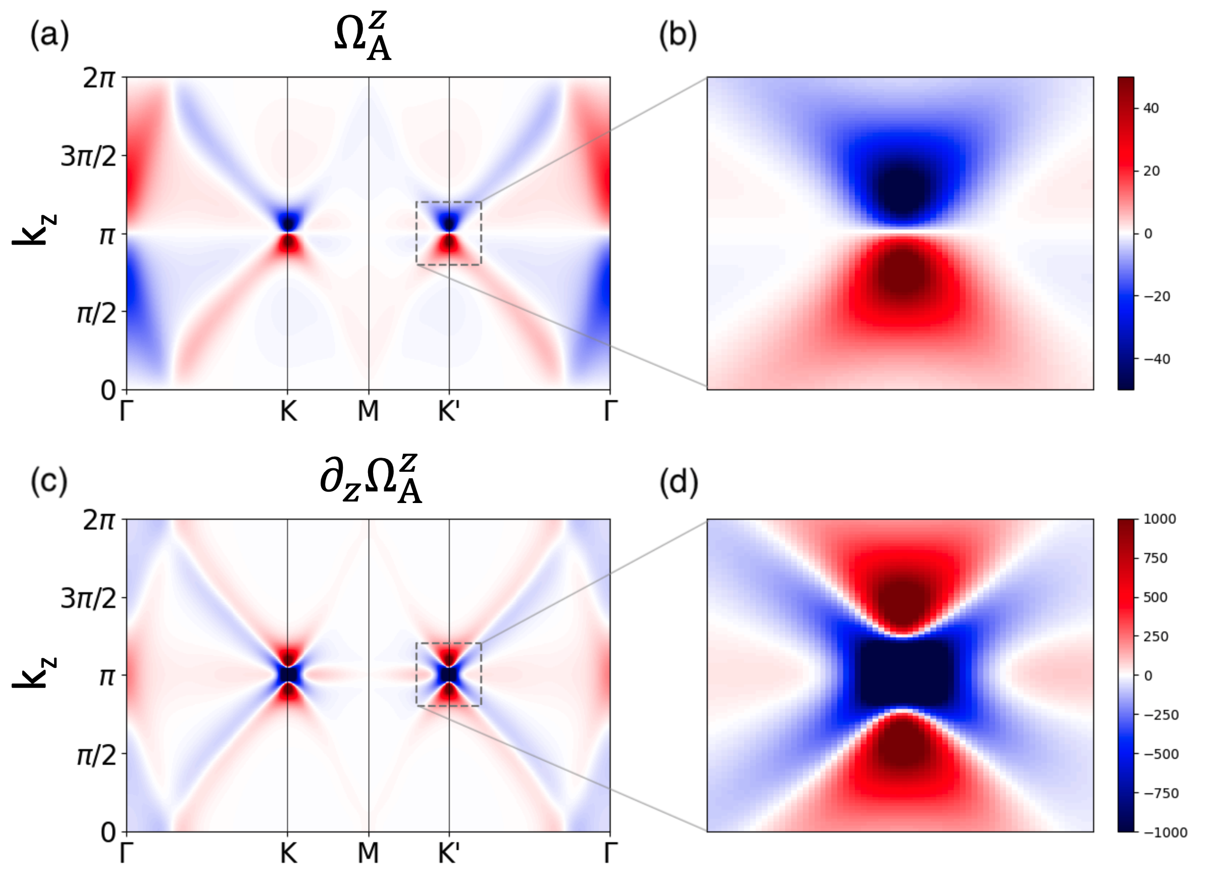
The electronic structure is calculated by employing the HSE06 hybrid functional Paier et al. (2006) implemented in the VASP code Kresse and Furthmüller (1996a, b); Kresse and Joubert (1999) . The maximaly localized Wannier functions are generated using Wannier90 Pizzi et al. (2020), and disentanglement is performed using a frozen window below $\varepsilon_{\rm F}+3{\rm eV}$ with $s,p$ orbitals of Te as projections. Tellurium has a band gap of about 0.3eV with conduction band (CB) minimum and valence band (VB) maximum around the H and H^′ points of the brillouin zone (BZ). The material is usually p-doped, and the VB presents more interest. However, for our demonstration the CB is more interesting because there is a Weyl point (WP) at the H point, which presents a computational challenge for the evaluation of Berry dipole via Eq. (77). Moreover, this WP is predicted to give a significant contribution to switch the sign of circular photogalvanic effect at high temperatures and low doping Tsirkin et al. (2018). The methodology derived in this manuscript has been implemented within the open-source code WanierBerriTsirkin (2021).

Figure 3: (c) Energy band of Tellurium, the k-path of which is a small range around H point of K-H-K line. There is a Weyl point (WP) at the H point located at 0.312eV above Fermi energy. (b)(d) Berry curvature z-component of the conduction band (CB) 1 and 2. (a)(e) Derivative of Berry curvature z-component of CB1 and CB2. Solid black lines are calculated with Eqs. (68b) and (68c). And the dashed color lines are calculated by the finite difference of Berry curvature.

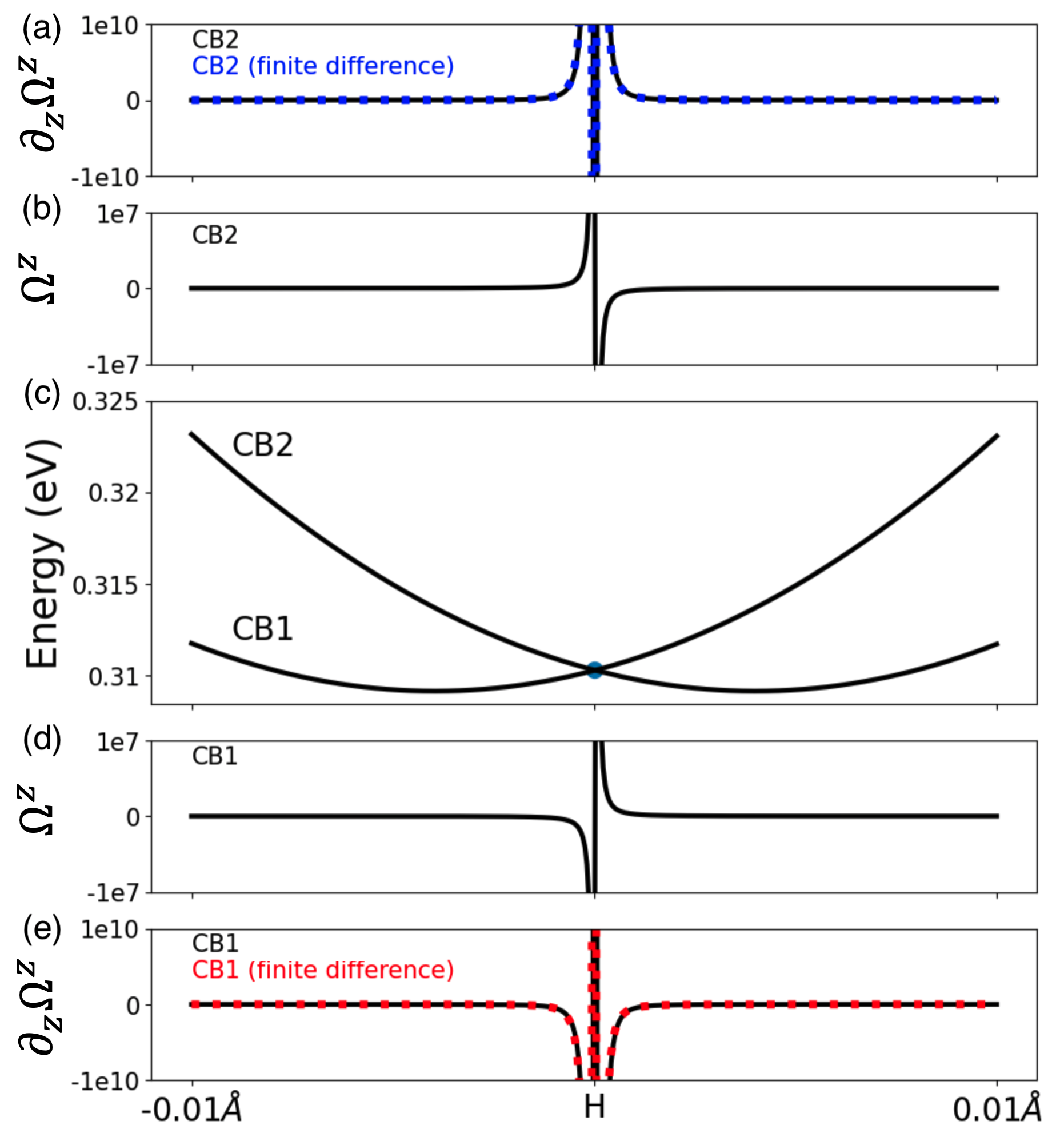
By using Wannier interpolation, the interpolated Berry curvature $\widetilde{\Omega}$ of conduction bands CB1 and CB2 can be calculated with

$$\widetilde{\Omega}^{c}_{n}=-\epsilon_{abc}{\rm Im}\widetilde{F}^{ab}_{nn}~{},$$ (75)

where $\widetilde{F}^{ab}_{nn}$ is introduced in Eq. (65a). According to Eq. (12), the Berry curvature of a single band follows an inverse-square law with respect to the energy difference with other bands, and therefore it changes rapidly in the vicinity of the WP, as shown in Fig. 3(b,d). Following Eq. (68a), the interpolated derivatives of Berry curvature are calculated with

$$\widetilde{\Omega}^{c:d}_{n}=-\epsilon_{abc}{\rm Im}\widetilde{F}^{ab:d}_{nn},$$ (76)

which are shown in Fig. 3(a,e) as solid lines. The dashed colored lines are plotted using finite differences based on the interpolated Berry curvature data in Fig. 3(b,d), using denser k sampling. The solid curves in Fig. 3(b,d) show good agreement with dashed colored lines, indicating that our Wannier interpolation method with covariant gradient works well around WPs in real materials.

Figure 4: (a)(c) Berry curvature z-component $\Omega^{z}_{\rm A}$ and derivative of Berry curvature zz-component $\partial_{z}\Omega^{z}_{\rm A}$ of all occupied bands below Weyl point (WP) energy on a plane submanifold of Brillouin zone. (b)(d) The zoom-in of the dashed square range in (a)(c).

In the previous research, evaluating ${\cal H}_{{\bf k}n}^{:a}\widetilde{\Omega}_{{\bf k}n}^{b}$ on the Fermi surface is a widely used method to calculate dimensionless Berry curvature dipole tensor via Eq. (77). Typically, one evaluates it as a direct summation

$$\mathcal{D}_{ab}^{\rm surf}=\frac{1}{N_{\bf k}V_{\rm u.c.}}\sum_{{\bf k}n}\partial_{a}\varepsilon_{{\bf k}n}\Omega_{{\bf k}n}^{b}\left(-\frac{\partial f_{0}}{\partial\varepsilon}\right)_{\varepsilon=\varepsilon_{{\bf k}n}}~{}.$$ (77)

However, at low temperature, the derivative of the distribution function with energy $f_{0}^{\prime}$ is a narrow peak function. This means only the k points that lie closely on the Fermi surface contribute to the integral. However, a big number of points needs to be evaluated before the narrow peaks from individual ${\bf k}$-points merge into a smooth curve. In Singh et al. (2020) $\mathcal{D}_{ab}$ was by first computing the Fermi surface by employing the tetrahedron method at a given k grid, and then the Berry curvature was sampled only at the reduced grid points near the Fermi surface. However, they also noted a slow convergence of the integral.

Instead, in (7) all k-points (which have bands below Fermi level) contribute, and therefore we are integrating a smoother function.

Another reason for the slow convergence of Eq. (77) is the sharp peak of the Berry curvature near a WP. Close to theWP the divergent part of the BC is equal in magnitude and opposite in sign for the two subbands. Therefore, if the Fermi level is above (below) both subbands, in the Fermi-sea integral the divergent parts cancel out (do not appear). In turn, in the Fermi-surface integral both subbands contribute with their divergent Berry curvature multiplied by different velocities and distribution functions, and therefore no cancellation occurs.

Figure 5: (a) Integral of Berry curvature dipole using Fermi surface Eq. (77) and Fermi sea Eq. (7) integral function. The colors show different k-points sampling numbers (unit M is million) in all Brillouin zone. WP is the energy where the Weyl point is located. (b) The standard deviation compared with the converged result.

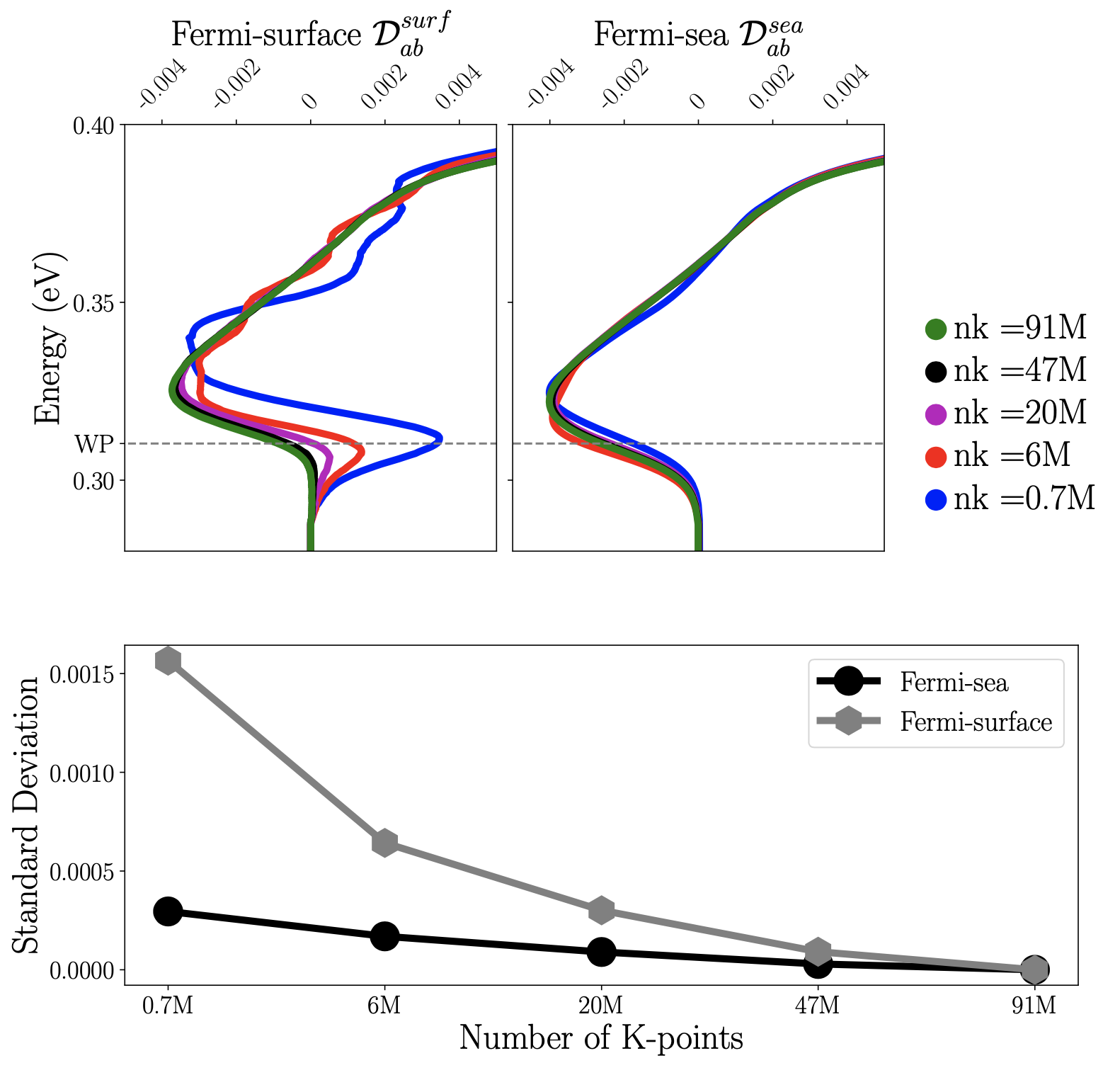
Thus, the Fermi-sea integral should have a better convergence with respect to the density of the ${\bf k}$-grid. To demonstrate this, we calculated the Berry dipole using both Eq. (77) and Eq. (7) at temperature 50K, as shown in Fig. 5(a), with varying numbers of k-points. When using Eq. (77) and a smaller number of k-points, there is a clear divergence in the Fermi-surface curve at the Weyl point energy. And the curve does not converge until 47 million k-points are used. In contrast, the Fermi-sea curve exhibits good convergence and is almost converged with only 0.7 million k-points, without any divergence at the Weyl point energy. The standard deviation of the results also supports these findings, as shown in Fig. 5(b).

VII Conclusions

In this paper, we present a Wannier interpolation scheme of the non-Abelian Berry curvature and orbital magnetic moment matrices for a group of bands. This method involves grouping the bands of interest together in specific energy range, which not only reduces computational complexity but also avoids convergence difficulties caused by intersections of bands within the group. By computing the trace of interpolated quantities, the sum of the quantities of the band in the group are obtained.

When studying higher-order transport phenomena using “Berry-Boltzmann equation”, we can use integration by parts to transfer the derivative from the distribution function to other quantities, thus converting the conversion from “Fermi surface” integration to “Fermi sea” integration. The advantage of “Fermi sea” integration is that all electron states below the Fermi level contribute to the integral, and there is no need to evaluate the Fermi surface with dense k-sampling, which results in fewer k-points needed to obtain accurate results. In our ab initio simulation of the Berry curvature dipole in Te, the “Fermi sea” integration demonstrates good stability and convergence compared to the “Fermi surface” integration.

However, the application of the developed method is not limited to improving convergence of a Berry curvature dipole. In the study of magnetotransport within Berry-Boltzmann formalism one gets terms where the derivatives of Berry curvature and orbital moment cannot be avoided. In particular, that allowed us to evaluate the recently measured Rikken and Avarvari (2019); Calavalle et al. (2022) electrical magnetochiral anisotropy (eMChA) in tellurium. These calculations are described in Liu et al.

Appendix A Tracelessness of Berry dipole

As noted before, Eq. (14) is symmetric under permutation of indices $b\leftrightarrow c$,

$$\Omega_{\rm A}^{ab,c}=\Omega_{\rm A}^{ac,b}\,.$$ (78)

To make sense of this symmetry, let us recast the Berry curvature an a pseudovector, $\Omega^{c}_{\rm A}=\epsilon_{abc}\Omega^{ab}_{\rm A}/2$. Applying $\partial_{c}$ to both sides of this relation and then using Eq. (78) gives

$${\boldsymbol{\nabla}}_{\bf k}\cdot{\boldsymbol{\Omega}}_{\rm A}=0\,.$$ (79)

Thus, the net Berry curvature of a group of states is divergence-free everywhere in the BZ. This is a known result for a single band, because Berry curvature is a curl of Berry connection ${\boldsymbol{\Omega}}_{n}=i{\boldsymbol{\nabla}}_{\bf k}\times\langle n|{\boldsymbol{\nabla}}_{\bf k}n\rangle$, and a divergence of a curl is always zero. This is true even at chiral touching points, where the Berry curvature of an individual band has nonzero divergence. The reason is that each chiral node acts as a monopole source of Berry curvature for one of the touching bands and as a sink for the other; but since degenerate states must belong to the same group A or B (recall that the two groups were assumed to be separated in energy), the monopoles cancel each other out. It follows from Eq. (79) that the “Berry curvature dipole’ tensor” (7) is always traceless. Moreover the integrand of Eq. (7) is traceless at every k-point, therefore the resulting tensor has a zero trace even if integration is done on a coarse ${\bf k}$-grid. In turn, the integrand of Eq. (77) is not traceless, therefore the tensor $\mathcal{D}_{cd}^{\rm surf}$ becomes traceless only after integration is performed with high precision. Naturally, in an accurate calculation $\mathcal{D}_{cd}^{\rm surf}=\mathcal{D}_{cd}^{\rm sea}$, however that level of precision is not always easy to achieve.

Appendix B Proof of chain rule

We assume that the function $f$ is smooth, and a Taylor expansion is valid:

$$f(x)=f_{0}+f_{1}x+f_{2}x^{2}+f_{3}x^{3}+f_{4}x^{4}+\ldots$$ (80)

Therefore $F_{ij}$ can be rewritten as

$$\widetilde{f}_{ij}=f_{0}+f_{1}{\cal H}_{ij}+f_{2}{\cal H}_{ii^{\prime}}{\cal H}_{i^{\prime}j}+f_{3}{\cal H}_{ii^{\prime}}{\cal H}_{i^{\prime}i^{\prime\prime}}{\cal H}_{i^{\prime\prime}j}+\ldots$$ (81)

Here we assume that $i,i^{\prime},i^{\prime\prime},\ldots,j$ all belong to the same subspace (A or B) Which will be valid in any gauge that does not mix the subspaces. Therefore, using the product rule we can easily take the generalized derivative

$$\widetilde{f}_{ij}^{:a}=f_{1}{\cal H}^{:a}_{ij}+f_{2}\left({\cal H}_{ii^{\prime}}^{:a}{\cal H}_{i^{\prime}j}+{\cal H}_{ii^{\prime}}{\cal H}_{i^{\prime}j}^{:a}\right)\\ +f_{3}\left({\cal H}_{ii^{\prime}}^{:a}{\cal H}_{i^{\prime}i^{\prime\prime}}{\cal H}_{i^{\prime\prime}j}+{\cal H}_{ii^{\prime}}{\cal H}_{i^{\prime}i^{\prime\prime}}^{:a}{\cal H}_{i^{\prime\prime}j}+{\cal H}_{ii^{\prime}}{\cal H}_{i^{\prime}i^{\prime\prime}}{\cal H}_{i^{\prime\prime}j}^{:a}\right)\\ +\ldots$$ (82)

Which in the Hamiltonian gauge is simplified to

$$\widetilde{f}_{ij}^{:a}={\cal H}^{:a}_{ij}\bigl{[}f_{1}+f_{2}(\varepsilon_{i}+\varepsilon_{j})+f_{3}(\varepsilon_{i}^{2}+\varepsilon_{i}\varepsilon_{j}+\varepsilon_{j}^{2})+\ldots\bigr{]}$$ (83)

In case $\varepsilon_{j}=\varepsilon_{j}=\varepsilon$ it reduces to

$$\widetilde{f}_{ij}^{:a}={\cal H}^{:a}_{ij}\bigl{[}f_{1}+2f_{2}\varepsilon+3f_{3}\varepsilon^{2}+\ldots\bigr{]}={\cal H}^{:a}_{ij}\frac{df(\varepsilon)}{d\varepsilon}$$ (84)

Now, if $\varepsilon_{i}\neq\varepsilon_{j}$, we can multiply and divide by $\varepsilon_{i}-\varepsilon_{j}$ and get

$$\widetilde{f}_{ij}^{:a}={\cal H}^{:a}_{ij}\cdot\tfrac{f_{1}(\varepsilon_{i}-\varepsilon_{j})+f_{2}(\varepsilon_{i}^{2}+\varepsilon_{j}^{2})+f_{3}(\varepsilon_{i}^{3}-\varepsilon_{j}^{3})+\ldots}{\varepsilon_{i}-\varepsilon_{j}}=\\ ={\cal H}^{:a}_{ij}\cdot\tfrac{f(\varepsilon_{i})-f(\varepsilon_{j})}{\varepsilon_{i}-\varepsilon_{j}}$$ (85)

Note, that in the limit $\varepsilon_{i}\to\varepsilon_{j}$ (85) reduces to (84)

Appendix C $\overline{B}$ inside the frozen window

From Eqs. (63) and (67b) it follows that

$$\overline{B}^{b}_{ln}=i\langle u_{l}|{\cal H}|\partial_{b}u_{j}^{\text{W}}\rangle U_{jn}$$ (86)

And, if

$${\cal H}|u_{l}\rangle=\varepsilon_{l}|u_{l}\rangle$$ (87)

then we may write

$$\overline{B}^{b}_{ln}=\varepsilon_{l}\overline{A}_{ln}^{b}$$ (88)

However, in Wannier interpolation Eq. (87) is true only if the energy $\varepsilon_{l}$ is inside the frozen window. Otherwise, the wavefunctions $|u_{l}\rangle$ are not guaranteed to be eigenstates of the Hamiltonianm although the columns of $U$ are eigenvectors of ${\cal H}^{\text{W}}$. Therefore, it is convenient, and computationally effective to evaluate $B^{b}_{ln}$ using Eq. (88) when $\varepsilon_{l}$ lies in the frozen window, and use Eqs. (63) and (67b) otherwise. However, such substitution becomes discontinuous at the points when a band crosses the borders of frozen window, which disables differentiation. So, we can intoroduce a smoothed version:

$$\widetilde{\overline{B}}{}^{b}_{ln}=f(\varepsilon_{l})\varepsilon_{l}\overline{A}^{b}_{ln}+(1-f(\varepsilon_{l}))\overline{B}^{b}_{ln}$$ (89)

Where $f(\varepsilon)$ is a smooth function, such that $f(\varepsilon)=1$ deep inside the frozen window, and $f(\varepsilon)=0$ far outside it. The width of the transition region should be chosen rather narrow, but finite. Now, in order to be to use the rules of covariant derivative, let us write it in covariant form as

$$\widetilde{\overline{B}}{}^{b}_{ln}=f_{ll^{\prime}}{\cal H}_{l^{\prime}l^{\prime\prime}}\overline{A}^{b}_{l^{\prime\prime}n}+(1-f_{ll^{\prime}})\overline{B}^{b}_{l^{\prime}n}$$ (90)

where $f_{ll^{\prime}}=\delta_{ll^{\prime}}f(\varepsilon_{l})$ To this equation we can directly apply the product rule (19) and get

$$\widetilde{\overline{B}}{}^{b;d}_{ln}=f_{ll^{\prime}}{\cal H}_{l^{\prime}l^{\prime\prime}}^{;d}\overline{A}^{b}_{l^{\prime\prime}n}+f^{;d}_{ll^{\prime}}{\cal H}_{l^{\prime}l^{\prime\prime}}\overline{A}^{b}_{l^{\prime\prime}n}-f^{;d}_{ll^{\prime}}\overline{B}^{b}_{l^{\prime}n}+\\ +f_{ll^{\prime}}{\cal H}_{l^{\prime}l^{\prime\prime}}\overline{A}^{b;d}_{l^{\prime\prime}n}+\bigl{(}1-f_{ll^{\prime}})\overline{B}^{b;d}_{l^{\prime}n}$$ (91)

where $f_{ll^{\prime}}$ is evaluated according to chainrule (20).

Appendix D Evaluation of matrices in Wanier gauge

$$\left(A^{\text{W}}\right)^{a}_{ij} \equiv i\langle u_{i}^{\text{W}}|\partial_{a}u_{j}^{\text{W}}\rangle$$ (92a)

$$= e^{i{\bf k}({\bf t}_{j}-{\bf t}_{i})}\sum_{\mathbf{R}}e^{i{\bf k}{\bf R}}\mathbb{A}^{a}_{ij}({\bf R})$$

$$\left(B^{\text{W}}\right)^{a}_{ij} \equiv i\langle u_{i}^{\text{W}}|{\cal H}|\partial_{a}u_{j}^{\text{W}}\rangle$$ (92b)

$$= e^{i{\bf k}({\bf t}_{j}-{\bf t}_{i})}\sum_{\mathbf{R}}e^{i{\bf k}\mathbf{R}}\mathbb{B}^{a}_{ij}({\bf R})$$

$$\left(H^{\text{W}}\right)^{ab}_{ij} \equiv \langle\partial_{a}u_{i}^{\text{W}}|{\cal H}|\partial_{b}u_{j}^{\text{W}}\rangle$$ (92c)

$$= e^{i{\bf k}({\bf t}_{j}-{\bf t}_{i})}\sum_{\mathbf{R}}e^{i{\bf k}\mathbf{R}}\mathbb{C}^{a}_{ij}({\bf R})$$

$$\left(F^{\text{W}}\right)^{ab}_{ij} \equiv \langle\partial_{a}u_{i}^{\text{W}}|\partial_{b}u_{j}^{\text{W}}\rangle$$ (92d)

$$= e^{i{\bf k}({\bf t}_{j}-{\bf t}_{i})}\sum_{\mathbf{R}}e^{i{\bf k}\mathbf{R}}\mathbb{F}^{ab}_{ij}({\bf R})$$

Where

$$\mathbb{A}^{a}_{ij}({\bf R}) = \langle\mathbf{0}i|\hat{r}_{a}-t_{j}^{a}|{\bf R}j\rangle$$ (93a)

$$\mathbb{B}^{a}_{ij}({\bf R}) = \langle\mathbf{0}i|{\cal H}\cdot(\hat{r}_{a}-\hat{R}_{a}-t_{j}^{a})|{\bf R}j\rangle$$ (93b)

$$\mathbb{C}^{ab}_{ij}({\bf R}) = \langle\mathbf{0}i|(\hat{r}_{a}-t_{i}^{a})\cdot{\cal H}\cdot(\hat{r}_{b}-t_{j}^{a}-\hat{R}_{b})|{\bf R}j\rangle$$ (93c)

$$\mathbb{F}^{ab}_{ij}({\bf R}) = \langle\mathbf{0}i|(\hat{r}_{a}-t_{i}^{a})\cdot(\hat{r}_{b}-t_{j}^{b}-\hat{R}_{b})|{\bf R}j\rangle$$ (93d)

These matrix elements can be computed using finite-difference schemes based on the ab initio bandstructures computed on regular ${\bf k}$-grids — a procedure that is widely described in the literature Marzari and Vanderbilt (1997); Wang et al. (2006); Lopez et al. (2012); Ryoo et al. (2019)

And the derivatives will be evaluated as

$$\partial_{d}\left(\cal{O}^{\text{W}}\right)_{ij}=ie^{i{\bf k}({\bf t}_{j}-{\bf t}_{i})}\sum_{\mathbf{R}}e^{i{\bf k}\mathbf{R}}\mathbb{O}_{ij}({\bf R})(R_{d}+t_{j}^{d}-t_{i}^{d})\\ =i(t_{j}^{d}-t_{i}^{d})\left(\cal{O}^{\text{W}}\right)_{ij}+ie^{i{\bf k}({\bf t}_{j}-{\bf t}_{i})}\sum_{\mathbf{R}}e^{i{\bf k}\mathbf{R}}\mathbb{O}_{ij}({\bf R})R_{d}\\$$ (94)

Appendix E Role of Wannier Centers

Interesting to note that quantities (93) were defined in Wang et al. (2006) and Lopez et al. (2012) (and in Wannier90 code) with ${\bf t}_{i}=0$. As far as inclusion of ${\bf t}$ in the phase factors correspond to a phase choice of the basis set, the computed physical observables should not depend on the value of $t$. Below we will show that the total value of $\widetilde{F}^{ab}_{mn}$ and $\widetilde{H}^{ab}_{mn}$ defined by Eqs. (65) and (66) does not depend on ${\bf t}_{i}$. However, the particular value of ”internal” and ”external” terms will depend on ${\bf t}$.

In particular, setting ${\bf t}_{i}$ equal to the the Wannier charge center $\langle 0j|\hat{{\bf r}}|0j\rangle$ will make $\widetilde{F}^{ab,\rm(ext)}_{mn}$ vanish in the ”tight-binding” limit, where $\langle{\bf R}i|\hat{{\bf r}}|{\bf R}^{\prime}j\rangle=\delta_{{\bf R}{\bf R}^{\prime}}\delta_{ij}$. Also, in the ab initio calculations, the computationally heavy ”external” terms become smaller with this choice,thus allowing to evaluate them on a coarser grid, to achieve the same absolute accuracy of the total Berry curvature.

Denoting qqunatities defined by Eqs. 92 at ${\bf t}_{i}=0$ as $\breve{\mathbb{A}}$, $\breve{\mathbb{B}}$, $\breve{\mathbb{C}}$, $\breve{\mathbb{F}}$ we find the following relations:

$$\mathbb{A}^{a}_{ij}({\bf R}) = \breve{\mathbb{A}}^{a}_{ij}({\bf R})-\delta_{ij}\delta_{R,0}t_{j}^{a}$$ (95a)

$$\mathbb{B}^{a}_{ij}({\bf R}) = \breve{\mathbb{B}}^{a}_{ij}({\bf R})-\breve{\cal H}_{ij}({\bf R})t_{j}^{a}$$ (95b)

$$\mathbb{C}^{ab}_{ij}({\bf R}) = \breve{\mathbb{C}}^{ab}_{ij}({\bf R})-t_{i}^{a}\breve{\mathbb{B}}_{ij}^{b}({\bf R})-\breve{\mathbb{B}}_{ji}^{a*}(-{\bf R})t_{j}^{b}$$ (95c)

$$+t_{i}^{a}\breve{\cal H}_{ij}({\bf R})t_{j}^{b}$$

$$\mathbb{F}^{ab}_{ij}({\bf R}) = \breve{\mathbb{F}}^{ab}_{ij}({\bf R})-t_{i}^{a}\breve{\mathbb{A}}_{ij}^{b}({\bf R})-t_{j}^{b}\breve{\mathbb{A}}_{ij}^{a}({\bf R})$$ (95d)

$$+\delta_{ij}\delta_{{\bf R},0}t_{i}^{a}t_{i}^{b}$$

Defining $\overline{t}^{a}_{ij}=U^{*}_{j^{\prime}i}t_{j^{\prime}}^{a}U_{j^{\prime}i}$ in accordance with Eq. (63), we arrive at the following relationsfpr the bar quantities:

$$\overline{A}^{a}_{ij} = \breve{\overline{A}}^{a}_{ij}-\overline{t}^{a}_{ij}$$ (96a)

$$\overline{D}^{a}_{ij} = \breve{\overline{D}}^{a}_{ij}-i\overline{t}^{a}_{ij}$$ (96b)

$$\overline{B}^{a}_{ij} = \breve{\overline{B}}^{a}_{ij}-\breve{\overline{H}}_{ij^{\prime}}\overline{t}^{a}_{j^{\prime}j}$$ (96c)

$$\overline{C}^{ab}_{ij} = \breve{\overline{C}}^{ab}_{ij}-(\breve{\overline{B}}^{a\dagger})_{ij^{\prime}}\overline{t}^{b}_{j^{\prime}j}-\overline{t}^{a}_{ij^{\prime}}\breve{\overline{B}}^{b}_{j^{\prime}j}-\overline{t}^{a}_{ii^{\prime}}\breve{\overline{H}}_{i^{\prime}j^{\prime}}\overline{t}^{b}_{j^{\prime}j^{\prime}}$$ (96d)

$$\overline{F}^{ab}_{ij} = \breve{\overline{F}}^{ab}_{ij}-\breve{\overline{A}}^{a}_{ij^{\prime}}\overline{t}^{b}_{j^{\prime}j}-\overline{t}^{a}_{ij^{\prime}}\breve{\overline{A}}^{b}_{j^{\prime}j}-\overline{t}^{a}_{ij^{\prime}}\overline{t}^{b}_{j^{\prime}j}$$ (96e)

Note, that summation here is performed over all wannierised states $i^{\prime},j^{\prime}$, no matter to which set ($A$ or $B$) belong the states $i,j$. Substituting these relations into Eq. (65) it is straightforward to show that $\widetilde{F}^{ab}_{mn}=\breve{\widetilde{F}}^{ab}_{mn}$. However, for $\widetilde{F}^{ab}_{mn}$ we get

$$\widetilde{H}^{ab}_{mn}-\breve{\widetilde{H}}^{ab}_{mn}=t^{a}_{mm^{\prime}}\left(H_{m^{\prime}n^{\prime}}A_{n^{\prime}n}^{b}-B_{m^{\prime}n}^{b}\right)+\left({}_{m\leftrightarrow n}^{a\leftrightarrow b}\right)^{*}$$ (97)

However this differnece vanishes if we apply Eq. (88). We should note that the relation (88) is not automatically sattisfied upon Wanier interpolation, and therefore it is important to enforce it by hand, and follow the procedure prescribed by Appendix C

Due to independence of the final result on the values of ${\bf t}_{i}$, the definition of ”Wannier center” may be understood broadly — not only as the Wanier charge center $\langle 0j|\hat{{\bf r}}|0j\rangle$, but also, e.g., as the position of an atom, on which the Wannier function is located.

Appendix F Second derivative

Using product rule again with the quantities in Sec. V.3, the second covariant derivative of $\widetilde{F}^{ab}_{mn}$ and $\widetilde{H}^{ab}_{mn}$ are shown as following.

$$\widetilde{F}^{ab:de}_{mn} = \widetilde{F}^{ab:de}_{mn,\textrm{int}}+\widetilde{F}^{ab:de}_{mn,\textrm{ext}}$$ (98a)

$$\widetilde{F}^{ab:de}_{mn,\textrm{int}} = \left(D_{ml^{\prime}}^{a:e}D_{l^{\prime}n}^{b:d}+D_{ml^{\prime}}^{a}D_{l^{\prime}n}^{b:de}\right)+\left({}_{m\leftrightarrow n}^{a\leftrightarrow b}\right)^{*}$$ (98b)

$$\widetilde{F}^{ab:de}_{mn,\textrm{ext}} = -\Bigl{[}\Bigl{(}i\overline{A}^{a:e}_{ml^{\prime}}D^{b:d}_{l^{\prime}n}+i\overline{A}^{a}_{ml^{\prime}}D^{b:de}_{l^{\prime}n}$$ (98c)

$$+iD^{a:e}_{ml^{\prime}}\overline{A}^{b:d}_{l^{\prime}n}+iD^{a}_{ml^{\prime}}\overline{A}^{b:de}_{l^{\prime}n}$$

$$+\overline{A}_{mn^{\prime}}^{a:e}\overline{A}_{n^{\prime}n}^{b:d}+\overline{A}_{mn^{\prime}}^{a}\overline{A}_{n^{\prime}n}^{b:de}\Bigr{)}$$

$$+\left({}_{m\leftrightarrow n}^{a\leftrightarrow b}\right)^{*}\Bigr{]}+\overline{F}^{ab:de}_{mn}$$

$$\widetilde{H}^{ab:de}_{mn} = \widetilde{H}^{ab:de}_{mn,\textrm{int}}+\widetilde{H}^{ab:de}_{mn,\textrm{ext}}$$ (99a)

$$\widetilde{H}^{ab:de}_{mn,\textrm{int}} = -\Bigl{[}\Bigl{(}D_{ml^{\prime}}^{a:e}{{\cal H}_{l^{\prime}l^{\prime\prime}}}D_{l^{\prime\prime}n}^{b:d}+D_{ml^{\prime}}^{a}{\cal H}^{,e}_{l^{\prime}l^{\prime\prime}}D_{l^{\prime\prime}n}^{b:d}$$ (99b)

$$+D_{ml^{\prime}}^{a}{{\cal H}_{l^{\prime}l^{\prime\prime}}}D_{l^{\prime\prime}n}^{b:de}+D_{ml^{\prime}}^{a:e}{\cal H}_{l^{\prime}l^{\prime\prime}}^{,d}D_{l^{\prime\prime}n}^{b}\Bigl{)}$$

$$+\left({}_{m\leftrightarrow n}^{a\leftrightarrow b}\right)^{*}\Bigr{]}-D_{ml^{\prime}}^{a}{\cal H}_{l^{\prime}l^{\prime\prime}}^{,d:e}D_{l^{\prime\prime}n}^{b}$$

$$\widetilde{H}^{ab:de}_{mn,\textrm{ext}} = \Bigl{[}\Bigl{(}i(\overline{B}^{\dagger})^{a:e}_{ml^{\prime}}D^{b:d}_{l^{\prime}n}+i(\overline{B}^{\dagger})^{a}_{ml^{\prime}}D^{b:de}_{l^{\prime}n}$$ (99c)

$$+iD^{a:e}_{ml^{\prime}}\overline{B}^{b:d}_{l^{\prime}n}+iD^{a}_{ml^{\prime}}\overline{B}^{b:de}_{l^{\prime}n}$$

$$-\overline{A}_{mm^{\prime}}^{a:e}{\cal H}_{m^{\prime}n^{\prime}}\overline{A}_{n^{\prime}n}^{b:d}-\overline{A}_{mm^{\prime}}^{a}{\cal H}^{,e}_{m^{\prime}n^{\prime}}\overline{A}_{n^{\prime}n}^{b:d}$$

$$-\overline{A}_{mm^{\prime}}^{a}{\cal H}_{m^{\prime}n^{\prime}}\overline{A}_{n^{\prime}n}^{b:de}-\overline{A}_{mm^{\prime}}^{a:e}{\cal H}_{m^{\prime}n^{\prime}}^{,d}\overline{A}_{n^{\prime}n}^{b}\Bigl{)}$$

$$+\left({}_{m\leftrightarrow n}^{a\leftrightarrow b}\right)^{*}\Bigr{]}-\overline{A}_{mm^{\prime}}^{a}{\cal H}_{m^{\prime}n^{\prime}}^{,d:e}\overline{A}_{n^{\prime}n}^{b}+\overline{H}^{ab:de}_{mn}$$

The derivatives $\overline{A}^{b:de}_{ln}$, $\overline{B}^{b:de}_{ln}$, $\overline{H}^{b:de}_{ln}$ and $\overline{F}^{b:de}_{ln}$ are evaluated in a general way. Take the covariant derivative agian of Eq. (70) following the pruduct rule, for instance reads

$$\overline{\cal O}^{:de}_{nn^{\prime}} = \overline{\cal O}^{,d:e}_{nn^{\prime}}-\sum_{l}^{B}D^{d:e}_{nl}{\cal O}_{ln^{\prime}}-\sum_{l}^{B}D^{d}_{nl}{\cal O}^{:e}_{ln^{\prime}}$$ (101)

$$+\sum_{l}^{B}{\cal O}^{:e}_{nl}D^{d}_{ln^{\prime}}+\sum_{l}^{B}{\cal O}_{nl}D^{d:e}_{ln^{\prime}}$$

And covariant matrix $D^{b:de}_{ln}$ reads

$$D^{b:de}_{ln} = \frac{1}{\varepsilon_{nl}}\Bigl{\{}{\cal H}^{,bd:e}_{ln}+\Bigl{[}\Bigl{(}{\cal H}^{,b:e}_{ll^{\prime}}D^{d}_{l^{\prime}n}+{\cal H}^{,b}_{ll^{\prime}}D^{d:e}_{l^{\prime}n}$$ (104)

$$-D^{d:e}_{ln^{\prime}}{\cal H}^{,b}_{n^{\prime}n}-D^{d}_{ln^{\prime}}{\cal H}^{,b:e}_{n^{\prime}n}\Bigl{)}+\Bigl{(}b\leftrightarrow d\Bigl{)}\Bigl{]}$$

$$+{\cal H}^{,e}_{ll^{\prime}}D^{b:d}_{ln^{\prime}}-D^{b:d}_{ln^{\prime}}{\cal H}^{,e}_{n^{\prime}n}\Bigl{\}}$$

References

• Tokura and Nagaosa (2018) Y. Tokura and N. Nagaosa, “Nonreciprocal responses from non-centrosymmetric quantum materials,” Nat. Commun. 9, 3740 (2018).
• Rikken et al. (2001) G. L. J. A. Rikken, J. Fölling,  and P. Wyder, “Electrical magnetochiral anisotropy,” Phys. Rev. Lett. 87, 236602 (2001).
• Avci et al. (2015) C. O. Avci, K. Garello, A. Ghosh, M. Gabureac, F. A. Santos,  and P. Gambardella, “Unidirectional spin Hall magnetoresistance in ferromagnet/normal metal bilayers,” Nat. Phys. 11, 570 (2015).
• Deyo et al. (2009) E Deyo, LE Golub, EL Ivchenko,  and B Spivak, “Semiclassical theory of the photogalvanic effect in non-centrosymmetric systems,” arXiv preprint arXiv:0904.1917  (2009), 10.48550/arXiv.0904.1917.
• Sodemann and Fu (2015) I. Sodemann and L. Fu, “Quantum nonlinear hall effect induced by berry curvature dipole in time-reversal invariant materials,” Phys. Rev. Lett. 115, 216806 (2015).
• Ma et al. (2019) Q. Ma, S.-Y. Xu, H. Shen, D. MacNeill, V. Fatemi, T.-R. Chang, A. M. Mier Valdivia, S. Wu, Z. Du, C.-H. Hsu, S. Fang, Q. D. Gibson, K. Watanabe, T. Taniguchi, R. J. Cava, E. Kaxiras, H.-Z. Lu, H. Lin, L. Fu, N. Gedik, ,  and P. Jarillo-Herrero, “Observation of the nonlinear Hall effect under time-reversal-symmetric conditions,” Nature 565, 337 (2019).
• Kang et al. (2019) K. Kang, T. Li, E. Sohn, J. Shan,  and K. F. Mak, “Nonlinear anomalous Hall effect in few-layer WTe2,” Nat. Mater. 18, 324 (2019).
• Huang et al. (2020) Meizhen Huang, Zefei Wu, Jinxin Hu, Xiangbin Cai, En Li, Liheng An, Xuemeng Feng, Ziqing Ye, Nian Lin, Kam Tuen Law,  and Ning Wang, “Giant nonlinear Hall effect in twisted WSe2,” arXiv e-prints , arXiv:2006.05615 (2020)arXiv:2006.05615 [cond-mat.mes-hall] .
• Zhang et al. (2020) C.-P. Zhang, X.-J. Gao, Y.-M. Xie, H. C. Po,  and K. T. Law, “Higher-Order Nonlinear Anomalous Hall Effects Induced by Berry Curvature Multipoles,” arXiv e-prints , arXiv:2012.15628 (2020).
• Xiao et al. (2010) D. Xiao, M.-.C. Chang,  and Q. Niu, “Berry phase effects on electronic properties,” Rev. Mod. Phys. 82, 1959 (2010).
• Gao (2019) Y. Gao, “Semiclassical dynamics and nonlinear charge current,” Front. Phys. 14, 33404 (2019).
• Morimoto et al. (2016) T. Morimoto, S. Zhong, J. Orenstein,  and J. E. Moore, “Semiclassical theory of nonlinear magneto-optical responses with applications to topological dirac/weyl semimetals,” Phys. Rev. B 94, 245121 (2016).
• Watanabe and Yanase (2020) H. Watanabe and Y. Yanase, “Nonlinear electric transport in odd-parity magnetic multipole systems: Application to Mn-based compounds,” Phys. Rev. Research 2, 043081 (2020).
• Nagaosa et al. (2010) N. Nagaosa, J. Sinova, S. Onoda, A. H. MacDonald,  and N. P. Ong, “Anomalous Hall effect,” Rev. Mod. Phys. 82, 1539 (2010).
• Železný et al. (2021) J. Železný, Z. Fang, K. Olejník, J. Patchett, F. Gerhard, C. Gould, L. W. Molenkamp, C. Gomez-Olivella, J. Zemen, T. Tichý, T. Jungwirth,  and C. Ciccarelli, “Unidirectional magnetoresistance and spin-orbit torque in nimnsb,” Phys. Rev. B 104, 054429 (2021).
• Parker et al. (2019) D. E. Parker, T. Morimoto, J. Orenstein,  and J. E. Moore, “Diagrammatic approach to nonlinear optical response with application to Weyl semimetals,” Phys. Rev. B 99, 045121 (2019).
• Lahiri et al. (2022) Shibalik Lahiri, Tanmay Bhore, Kamal Das,  and Amit Agarwal, “Nonlinear magnetoresistivity in two-dimensional systems induced by berry curvature,” Phys. Rev. B 105, 045421 (2022).
• Wang et al. (2006) X. Wang, J. R. Yates, I. Souza,  and D. Vanderbilt, “Ab initio calculation of the anomalous Hall conductivity by Wannier interpolation,” Phys. Rev. B 74, 195118 (2006).
• Yates et al. (2007) J. R. Yates, X. Wang, D. Vanderbilt,  and I. Souza, “Spectral and Fermi surface properties from Wannier interpolation,” Phys. Rev. B 75, 195121 (2007).
• Zhang et al. (2018a) Y. Zhang, Y. Sun,  and B. Yan, “Berry curvature dipole in Weyl semimetal materials: An ab initio study,” Phys. Rev. B 97, 041101 (2018a).
• Zhang et al. (2018b) Y. Zhang, J. van den Brink, C. Felser,  and B. Yan, “Electrically tuneable nonlinear anomalous Hall effect in two-dimensional transition-metal dichalcogenides WTe2 and MoTe2,” 2D Mater. 5, 044001 (2018b).
• He and Weng (2021) Zhihai He and Hongming Weng, “Giant Nonlinear Hall Effect in Twisted Bilayer WTe2,” npj Quantum Materials 6, 101 (2021).
• Vanderbilt (2018) D. Vanderbilt,  Berry Phases in Electronic Structure Theory: Electric Polarization, Orbital Magnetization and Topological Insulators (Cambridge University Press, Cambridge (United Kingdom), 2018).
• Aversa and Sipe (1995) Claudio Aversa and J. E. Sipe, “Nonlinear optical susceptibilities of semiconductors: Results with a length-gauge analysis,” Phys. Rev. B 52, 14636 (1995).
• Ventura et al. (2017) G. B. Ventura, D. J. Passos, J. M. B. Lopes dos Santos, J. M. Viana Parente Lopes,  and N. M. R. Peres, “Gauge covariances and nonlinear optical responses,” Phys. Rev. B 96, 035431 (2017).
• Lopez et al. (2012) M. G. Lopez, D. Vanderbilt, T. Thonhauser,  and I. Souza, “Wannier-based calculation of the orbital magnetization in crystals,” Phys. Rev. B 85, 014435 (2012).
• Chang and Niu (2008) Ming-Che Chang and Qian Niu, “Berry curvature, orbital moment, and effective quantum theory of electrons in electromagnetic fields,” Journal of Physics: Condensed Matter 20, 193202 (2008).
• Gao et al. (2015) Yang Gao, Shengyuan A. Yang,  and Qian Niu, “Geometrical effects in orbital magnetic susceptibility,” Phys. Rev. B 91, 214405 (2015).
• Marzari et al. (2012) Nicola Marzari, Arash A. Mostofi, Jonathan R. Yates, Ivo Souza,  and David Vanderbilt, “Maximally localized wannier functions: Theory and applications,” Rev. Mod. Phys. 84, 1419–1475 (2012).
• Wang et al. (2019) Chong Wang, Sibo Zhao, Xiaomi Guo, Xinguo Ren, Bing-Lin Gu, Yong Xu,  and Wenhui Duan, “First-principles calculation of optical responses based on nonorthogonal localized orbitals,” New Journal of Physics 21, 093001 (2019).
• Jin et al. (2021) Gan Jin, Daye Zheng,  and Lixin He, “Calculation of berry curvature using non-orthogonal atomic orbitals,” Journal of Physics: Condensed Matter 33, 325503 (2021).
• Paier et al. (2006) Joachim Paier, Martijn Marsman, K Hummer, Georg Kresse, Iann C Gerber,  and János G Ángyán, “Screened hybrid density functionals applied to solids,” The Journal of chemical physics 124, 154709 (2006).
• Kresse and Furthmüller (1996a) Georg Kresse and Jürgen Furthmüller, “Efficient iterative schemes for ab initio total-energy calculations using a plane-wave basis set,” Phys. Rev. B 54, 11169 (1996a).
• Kresse and Furthmüller (1996b) Georg Kresse and Jürgen Furthmüller, “Efficiency of ab-initio total energy calculations for metals and semiconductors using a plane-wave basis set,” Computational materials science 6, 15–50 (1996b).
• Kresse and Joubert (1999) Georg Kresse and Daniel Joubert, “From ultrasoft pseudopotentials to the projector augmented-wave method,” Phys. Rev. B 59, 1758 (1999).
• Pizzi et al. (2020) Giovanni Pizzi, Valerio Vitale, Ryotaro Arita, Stefan Blügel, Frank Freimuth, Guillaume Géranton, Marco Gibertini, Dominik Gresch, Charles Johnson, Takashi Koretsune, et al., “Wannier90 as a community code: new features and applications,” J. Phys. Condens. Matter 32, 165902 (2020).
• Tsirkin et al. (2018) Stepan S. Tsirkin, Pablo Aguado Puente,  and Ivo Souza, “Gyrotropic effects in trigonal tellurium studied from first principles,” Phys. Rev. B 97, 035158 (2018).
• Tsirkin (2021) Stepan S Tsirkin, “High performance wannier interpolation of berry curvature and related quantities with wannierberri code,” npj Computational Materials 7, 1–9 (2021).
• Singh et al. (2020) Sobhit Singh, Jinwoong Kim, Karin M. Rabe,  and David Vanderbilt, “Engineering weyl phases and nonlinear hall effects in ${\mathrm{t}}_{d}$-${\mathrm{mote}}_{2}$,” Phys. Rev. Lett. 125, 046402 (2020).
• Rikken and Avarvari (2019) G. L. J. A. Rikken and N. Avarvari, “Strong electrical magnetochiral anisotropy in tellurium,” Phys. Rev. B 99, 245153 (2019).
• Calavalle et al. (2022) Francesco Calavalle, Manuel Suárez-Rodríguez, Beatriz Martín-García, Annika Johansson, Diogo C Vaz, Haozhe Yang, Igor V Maznichenko, Sergey Ostanin, Aurelio Mateo-Alonso, Andrey Chuvilin, et al., “Gate-tuneable and chirality-dependent charge-to-spin conversion in tellurium nanowires,” Nature Materials 21, 526–532 (2022).
• (42) Xiaoxiong Liu, Ivo Souza,  and Stepan S. Tsirkin, “Electrical magnetochiral anisotropy with in trigonal tellurium from first principles,” in preparation .
• Marzari and Vanderbilt (1997) N. Marzari and D. Vanderbilt, “Maximally localized generalized wannier functions for composite energy bands,” Phys. Rev. B 56, 12847 (1997).
• Ryoo et al. (2019) Ji Hoon Ryoo, Cheol-Hwan Park,  and Ivo Souza, “Computation of intrinsic spin hall conductivities from first principles using maximally localized wannier functions,” Phys. Rev. B 99, 235113 (2019).