Semicontraction and Synchronization of Kuramoto-Sakaguchi Oscillator Networks

Abstract

This paper studies the celebrated Kuramoto-Sakaguchi model of coupled oscillators adopting two recent concepts. First, we consider appropriately-defined subsets of the $n$-torus called winding cells. Second, we analyze the semicontractivity of the model, i.e., the property that the distance between trajectories decreases when measured according to a seminorm. This paper establishes the local semicontractivity of the Kuramoto-Sakaguchi model, which is equivalent to the local contractivity for the reduced model. The reduced model is defined modulo the rotational symmetry. The domains where the system is semicontracting are convex phase-cohesive subsets of winding cells. Our sufficient conditions and estimates of the semicontracting domains are less conservative and more explicit than in previous works. Based on semicontraction on phase-cohesive subsets, we establish the at most uniqueness of synchronous states within these domains, thereby characterizing the multistability of this model.

I Introduction

When a group of dynamical agents interact and adapt their behavior to their neighbors’ state, collective dynamics can emerge. Synchronization is one such phenomenon, where all agents start following identical trajectories. Collective dynamics in general, and synchronization in particular, have been a major topic of research for centuries [1, 2, 3, 4] and still are an active field of research.

Among the effort in the scientific analysis of synchronization, a breakthrough occurred through the work of Kuramoto [4], building on the formalism of Winfree [3]. Shortly after, Sakaguchi, Shinomoto, and Kuramoto introduced the Kuramoto-Sakaguchi model [5], covering a larger class of dynamical systems. The impact of these models on the research in dynamical system is still vivid nowadays [6] and the multistability phenomenon is widely studied [7, 8, 9]. Over the last decades, various analyses of phase oscillator networks have been performed, leveraging a diversity of mathematical tools. Among these tools, contraction theory remains under-exploited, mostly due to the technical burdens to its applicability to oscillator networks [10] and a lack of knowledge about refined notions of contraction.

As discussed originally in [11], strongly contracting dynamical systems have numerous properties (e.g., global exponential stability of a unique equilibrium point and the existence of Lyapunov functions [12]), are finding increasingly widespread applications (e.g., in controls [13] and learning [14]), and their study is receiving increasing attention [13, 15, 16]. However, numerous example systems fail to satisfy this strong property and exhibit richer dynamics; examples include systems with symmetries or conserved quantities. In an attempt to tackle wider classes of systems, variations of contraction were developed over the years, such as transverse contraction [17], horizontal contraction [18], or $k$-contraction [19]. Starting with the work on partial [10] and horizontal [18] contraction, a theory of semicontractivity, i.e., contractivity with respect to seminorms, is now available [20, 21].

In this manuscript, we apply semicontraction theory to the Kuramoto-Sakaguchi model on complex networks, and we show that semicontraction naturally allows us to deal with the symmetries of such systems. Our first contribution (Thm 3) is to provide an accurate estimate (Fig. 2) of the regions of the state space where networks of Kuramoto-Sakaguchi oscillators are semicontracting. Theorem 3 improves similar approximations presented in Refs. [22, 23], in that it is more general, less conservative, and the estimate we obtain clearly emphasizes the role of network structures and parameters on the system’s behavior (Fig. 3). Furthermore, our proof is significantly more streamlined than the ones in [22, 23] and generalizable to a wider class of systems.

As an application of the semicontractivity results in Theorem 3, we then identify regions of the state spaces containing at most a unique synchronous state (Theorem 4), recovering the main results of Refs. [22, 23]. While previous analyses of existence and uniqueness of synchronous states were very ad hoc [22, 23], our proofs are generalizable and shed some light on the fundamental reasons leading to at most uniqueness, i.e., the local semicontractivity of the dynamics.

The key analytical and computational advantage of semicontraction theory is that it allows one to perform computations on the original vector field, without the need to obtain and then manipulate an explicit expression for the reduced dynamics. This advantage leads to our very concise proof of semicontractivity (see the proofs of Lemma 1, Lemma 2 and Theorem 3).

In the following, we first review the Kuramoto-Sakaguchi model (Sec. II) as well as semicontraction theory (Sec. III). Our main semicontractivity and at most uniqueness results are presented in Secs. IV and V respectively.

II The Kuramoto-Sakaguchi model on complex graphs

Let ${\cal G}$ denote a weighted, undirected, connected graph with $n$ vertices and $m$ edges. The matrices $B\in\mathbb{R}^{n\times m}$, ${\cal A}\in\mathbb{R}^{m\times m}$, and $L_{{\cal G}}=B{\cal A}B^{\top}$ are the incidence, weight, and Laplacian matrices of ${\cal G}$ respectively. The Laplacian’s eigenvalues are $0=\lambda_{1}(L_{{\cal G}})<\lambda_{2}(L_{{\cal G}})\leq\ldots\leq\lambda_{n}(L_{{\cal G}})$, and $\lambda_{2}(L)$ is known as the algebraic connectivity of ${\cal G}$ [24]. $\bm{1}_{n}\in\mathbb{R}^{n}$ is the vector with all components equal to one and $I_{n}\in\mathbb{R}^{n\times n}$ is the identity matrix.

A simple path in ${\cal G}$ is a sequence of vertices $p=(i_{1},...,i_{\ell})$, such that each consecutive pair is connected in ${\cal G}$ and each vertex appears at most once in $\sigma$. A cycle of ${\cal G}$ is a simple path whose ends ($i_{1}$ and $i_{\ell}$) are connected, and we denote it as $\sigma=(i_{0},i_{1},...,i_{\ell}=i_{0})$.

II-A The Kuramoto-Sakaguchi model

We consider the Kuramoto-Sakaguchi model [5] over a weighted undirected graph ${\cal G}$ with frustration parameter $\varphi\in[0,\pi/2]$,

$$\dot{x}_{i} =f_{i}(\bm{x})\coloneqq\omega_{i}-\sum_{j=1}^{n}a_{ij}\left[\sin(x_{i}-x_{j}-\varphi)+\sin\varphi\right],$$ (1)

where $\omega_{i}\in\mathbb{R}$ is the natural frequency of agent $i$ and $a_{ij}$ is the weight of the edge between $i$ and $j$.

Due to the rotational invariance of Eq. (1), the Kuramoto-Sakaguchi model is often considered as evolving on the $n$-torus. In our case, however, it will be more convenient to look at it as evolving in the Euclidean space $\mathbb{R}^{n}$. The diffusive nature of the couplings in Eq. (1) implies that adding a constant value to each degree of freedom leaves the dynamics invariant. The Kuramoto-Sakaguchi model is then invariant along the subspace ${\rm span}(\bm{1}_{n})$ and can be analyzed on $\bm{1}_{n}^{\perp}$ only.

We will need to distinguish the even and odd parts of the couplings between agents,

$$\dot{x}_{i} =\omega_{i}-\sum_{j=1}^{n}c_{ij}\sin(x_{i}-x_{j})-\sum_{j=1}^{n}s_{ij}\left[1-\cos(x_{i}-x_{j})\right]$$

$$=\omega_{i}+f^{\rm o}_{i}(\bm{x})+f^{\rm e}_{i}(\bm{x})\,,$$ (2)

where we defined $c_{ij}=a_{ij}\cos(\varphi)$ and $s_{ij}=a_{ij}\sin\varphi$.

A (frequency) synchronous state is an $\bm{x}^{\rm s}\in\mathbb{R}^{n}$ such that

$$f_{i}(\bm{x}^{\rm s}) =\omega_{i}+f^{\rm o}_{i}({\bm{x}}^{\rm s})+f^{\rm e}_{i}({\bm{x}}^{\rm s})=\omega^{\rm s}\,,$$ (3)

for some synchronous frequency $\omega^{\rm s}\in\mathbb{R}$. Whereas a synchronous state is not necessarily an equilibrium of Eq. (1), it evolves along the invariant direction of the system, $\bm{x}^{\rm s}+{\rm span}(\bm{1}_{n})$. Therefore, if for some time $t_{0}$, the system reaches a synchronous state $\bm{x}(t_{0})=\bm{x}^{\rm s}$, then it remains synchronous for all time, i.e., for all $t>t_{0}$,

$$\bm{x}(t) =\bm{x}^{\rm s}+(t-t_{0})\omega^{\rm s}\bm{1}_{n}\,.$$ (4)

II-B Winding cells and cohesive sets

Over the last decades, a variety of tools have been introduced to refine the analysis of Kuramoto oscillators networks. We present here some of these tools, that will be useful later. We refer to Ref. [22] for a comprehensive introduction to the following concepts.

Counterclockwise difference. To account for the toroidal topology of the state space of Eq. (1), we defined the counterclockwise difference [22] between two numbers $x_{1},x_{2}\in\mathbb{R}$,

$$d_{\rm cc}(x_{1},x_{2}) =x_{1}-x_{2}+2\pi k\,,$$ (5)

where $k\in\mathbb{Z}$ is such that $d_{\rm cc}(x_{1},x_{2})\in[-\pi,\pi)$. One notices that Eq. (1) is invariant under substitution of $d_{\rm cc}(x_{1},x_{2})$ for $x_{1}-x_{2}$.

Winding numbers and vectors. Given a cycle $\sigma=(i_{0},i_{1},...,i_{\ell}=i_{0})$ of the interaction graph, we define the winding number associated to $\bm{x}\in\mathbb{R}^{n}$,

$$q_{\sigma}(\bm{x}) =\frac{1}{2\pi}\sum\nolimits_{j=1}^{\ell}d_{\rm cc}(x_{i_{j-1}},x_{i_{j}})\in\mathbb{Z}\,.$$ (6)

A collection of cycles $\Sigma=(\sigma_{1},...,\sigma_{c})$ of ${\cal G}$ induces the associated winding vector,

$$q_{\Sigma}(\bm{x}) =[q_{\sigma_{1}}(\bm{x}),...,q_{\sigma_{c}}(\bm{x})]^{\top}\in\mathbb{Z}^{c}\,.$$ (7)

Winding cells. Equation (7) associates an element of the discrete space $\mathbb{Z}^{c}$ to any point $\bm{x}\in\mathbb{R}^{n}$. Reversing the map naturally defines a partition of $\mathbb{R}^{n}$ into winding cells,

$$\Omega_{\Sigma}(\bm{u}) =\left\{\bm{x}\in\mathbb{R}^{n}\colon q_{\Sigma}(\bm{x})=\bm{u}\right\}\,, \bm{u}\in\mathbb{Z}^{c}\,.$$ (8)

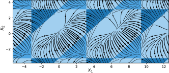
It is shown in Ref. [22] that, considered as a partition of the $n$-torus, winding cells are connected subsets of $\mathbb{T}^{n}$. As we are working in $\mathbb{R}^{n}$, winding cells are periodic copies of (dynamically) equivalent connected sets (see Fig. 1).

Figure 1: The Kuramoto-Sakaguchi vector field on the complete graph over 3 nodes. Only the first two components $(\dot{x}_{1},\dot{x}_{2})$ of the vector field are shown in the $(x_{1},x_{2},0)$ slice of $\mathbb{R}^{3}$. The background color illustrates the winding number [see Eq. (6)] at the corresponding point of the state space (light blue: $q=0$, medium blue: $q=+1$, dark blue: $q=-1$). The set of points sharing the same color then belong to the same winding cell. One readily sees that both the vector field and the winding numbers are $2\pi$-periodic in all dimensions. We refer to [22, 23] for 3-dimensional visualizations of winding cells.

Cohesive sets. For $\gamma\in[0,\pi]$, a state $\bm{x}\in\mathbb{R}^{n}$ is $\gamma$-cohesive if for each edge $(i,j)$ of ${\cal G}$, $|d_{\rm cc}(x_{i},x_{j})|\leq\gamma$. The $\gamma$-cohesive set, $\Delta_{{\cal G}}(\gamma)$, gathers all cohesive states, and the $\gamma$-cohesive $\bm{u}$-winding cell is

$$\Gamma({\bm{u},\gamma}) =\Omega_{\Sigma}(\bm{u})\cap\Delta_{{\cal G}}(\gamma)\,.$$ (9)

The set $\Gamma({\bm{u},\gamma})$ will be our semicontractive domain for the Kuramoto-Sakaguchi model.

III Semicontraction theory

We now review semicontraction theory, focusing on the notions needed to prove semicontractivity of the Kuramoto-Sakaguchi model. We refer to [16, Chap. 5] for a comprehensive presentation and to [21] for recent advances.

A seminorm is a function $\|\cdot\|\colon\mathbb{R}^{n}\to\mathbb{R}$ satisfying

$$\|\alpha x\| =|\alpha|\cdot\|x\| \alpha \in\mathbb{R}\,,$$ (10)

$$\|x+y\| \leq\|x\|+\|y\|\,.$$ (11)

Each seminorm has a kernel, i.e., a vector subspace where the seminorm vanishes. Each seminorm is a norm when restricted to the subspace perpendicular to the kernel.

The Kuramoto-Sakaguchi model being invariant under homogeneous angle shifts, we consider seminorms whose kernel is the consensus space $\operatorname{span}(\bm{1}_{n})$. Let $R\in\mathbb{R}^{(n-1)\times n}$ be a full rank matrix whose rows form an orthonormal basis of the subspace $\bm{1}_{n}^{\perp}$, and define the orthogonal projection

$$\Pi_{n} =R^{\top}R=I_{n}-n^{-1}\bm{1}_{n}\bm{1}_{n}^{\top}\,.$$ (12)

In what follows we consider the $(\ell_{2},\Pi_{n})$ consensus seminorm defined by $\|\bm{x}\|_{2,\Pi_{n}}=\|\Pi_{n}\bm{x}\|_{2}=\|R\bm{x}\|_{2}$. This choice of seminorm is somewhat arbitrary, but will be justified a posteriori by the results it will allow.

Each (semi)norm $\|\cdot\|$ naturally induces a matrix (semi)norm, itself inducing the matrix logarithmic (semi)norm [20, Def. 4] [16, Secs. 2.4 & 5.3]

$$\mu(A) \coloneqq\lim_{h\to 0^{+}}\frac{\|I_{n}+hA\|-1}{h}\,.$$ (13)

We denote the logarithmic seminorm induced by the consensus seminorm as $\mu_{2,\Pi_{n}}$. Logarithmic (semi)norms enjoy the following basic and well known properties:

$$\mu(\alpha A) =\alpha\mu(A) \alpha \geq 0\,,$$ (14)

$$\mu(A+B) \leq\mu(A)+\mu(B)\,,$$ (15)

$$\mu(A) \leq\|A\|\,.$$ (16)

When a seminorm is induced by a full-rank matrix $R$, the corresponding logarithmic seminorm satisfies [20, Theorem 6]

$$\mu_{R}(A) =\mu(RAR^{\dagger})\,,$$ (17)

with $\dagger$ denoting the Moore-Penrose pseudoinverse [25, Ex. 7.3.P7]. In addition to Eq. (17), here are two other ways of computing the consensus logarithmic seminorm of a matrix:

$$\mu_{2,\Pi_{n}}(A) =\lambda_{\max}\left(R\frac{A+A^{\top}}{2}R^{\dagger}\right)\,,$$ (18)

$$\mu_{2,\Pi_{n}}(A) =\min\left\{b\colon\Pi_{n}A+A^{\top}\Pi_{n}\preceq 2b\Pi_{n}\right\}\,,$$ (19)

where $\lambda_{\max}$ denotes the largest eigenvalue of a matrix. Equation (18) follows from inserting Eq. (17) and the property $R^{\dagger}=R^{\top}$ into the second line of [16, Tab. 2.1]. Equation (19) follows from [16, Lem. 5.8]. A remarkable consequence of Eq. (19) is that, when $L_{{\cal G}}$ is a weighted Laplacian matrix,

$$\mu_{2,\Pi_{n}}(-L_{{\cal G}}) =-\lambda_{2}(L_{{\cal G}})\,.$$ (20)

We are now ready to define (semi)contraction. A dynamical system $\dot{x}=g(x)$ over a convex domain $C\in\mathbb{R}^{n}$ is said to be strongly infinitesimally (semi)contracting [20, Def. 12] [16, Defs. 3.8 & 5.9] if the logarithmic (semi)norm of its Jacobian is upper bounded by a negative constant everywhere in $C$,

$$\mu(D{g}(x)) \leq-c\,,~{}\forall x\in C\,,$$ (21)

and $c>0$ is the (semi)contraction rate. For an illustration of a semicontractive system, we refer to [16, Figs. 5.3 and 5.4].

IV Infinitesimal semicontraction in the phase-cohesive winding cells

The rotational invariance of the Kuramoto-Sakaguchi model implies that the system cannot be semicontracting everywhere in $\mathbb{R}^{n}$. Our only hope is then to find subsets of $\mathbb{R}^{n}$ where the system is semicontracting.

Let us define the odd and even Jacobian matrices

$$\left[D\!{f^{\rm o}}(\bm{x})\right]_{ij} =\left\{\begin{array}[]{ll}c_{ij}\cos(x_{i}-x_{j})\,,&i\neq j\,,\\ -\sum_{k=1}^{n}c_{ik}\cos(x_{i}-x_{k})\,,&i=j\,,\end{array}\right.$$ (24)

$$\left[D\!{f^{\rm e}}(\bm{x})\right]_{ij} =\left\{\begin{array}[]{ll}-s_{ij}\sin(x_{i}-x_{j})\,,&i\neq j\,,\\ \sum_{k=1}^{n}s_{ik}\sin(x_{i}-x_{k})\,,&i=j\,,\end{array}\right.$$ (27)

and the Jacobian matrix of Eq. (1)

$$D\!{f} =D\!{f^{\rm o}}+D\!{f^{\rm e}}\,.$$ (28)

Note that all three Jacobians above have zero row sum, the same sparsity pattern as $L_{{\cal G}}$, and that $D\!{f^{\rm o}}$ is symmetric.

By subadditivity of the logarithmic seminorms [Eq. (15)], we can analyze the odd and even parts of $f$ independently. The two following lemmas provide bounds on the logarithmic seminorm of the odd and even Jacobians respectively.

Lemma 1 (Log-seminorm of the odd Jacobian)

For any $\gamma$-cohesive state $\bm{x}\in\Delta_{{\cal G}}(\gamma)$, the logarithmic seminorm of the odd Jacobian (24) is bounded as

$$\mu_{2,\Pi_{n}}(D\!{f^{\rm o}}(\bm{x})) \leq-\cos(\varphi)\cos(\gamma)\lambda_{2}(L_{{\cal G}})\,,$$ (29)

where $\lambda_{2}(L_{{\cal G}})$ is the algebraic connectivity of the graph ${\cal G}$.

Proof:

We notice that, under our assumptions, $-D\!{f^{\rm o}}$ is a symmetric Laplacian matrix with positive edge weights. Eq. (20) then implies

$$\mu_{2,\Pi_{n}}(D\!{f^{\rm o}}(\bm{x})) =\lambda_{2}(D\!{f^{\rm o}})\,.$$ (30)

Now, let us take $\bm{x}\in\Delta_{{\cal G}}(\gamma)$, for $\gamma\in[0,\pi/2]$. Then, each off-diagonal term ($i\neq j$) of the Jacobian $D\!{f^{\rm o}}(\bm{x})$ satisfies

$$0 \leq a_{ij}\cos(\varphi)\cos(\gamma)\leq\left(D\!{f^{\rm o}}(\bm{x})\right)_{ij}\leq a_{ij}\cos(\varphi)\,,$$ (31)

with the $a_{ij}$’s being the elements of the adjacency matrix of ${\cal G}$. Let us define the symmetric matrix

$$L(\bm{x}) =D\!{f^{\rm o}}(\bm{x})+\cos(\varphi)\cos(\gamma)L_{{\cal G}}\,.$$ (32)

By Eq. (31), $L(\bm{x})$ has nonnegative off-diagonal elements, zero row sum, and therefore nonpositive diagonal elements (it is a Laplacian matrix). Hence, by Gershgorin Circles Theorem [25, Theorem 6.1.1], $L(\bm{x})$ is negative semidefinite. Using a corollary of Weyl’s inequality [25, Cor. 4.3.12],

$$-\lambda_{2}(D\!{f^{\rm o}}(\bm{x})) =\lambda_{2}\left(\cos(\varphi)\cos(\gamma)L_{{\cal G}}-L(\bm{x})\right)$$

$$\geq\cos(\varphi)\cos(\gamma)\lambda_{2}(L_{{\cal G}})$$ (33)

which concludes the proof. ∎

Lemma 2 (Log-seminorm of the even Jacobian)

For any $\gamma$-cohesive point $\bm{x}\in\Delta_{{\cal G}}(\gamma)$, the logarithmic seminorm of the even Jacobian (27) is bounded as

$$\mu_{2,\Pi_{n}}(D\!{f^{\rm e}}(\bm{x})) \leq\sin(\varphi)\sin(\gamma)d_{\max}\,.$$ (34)

where $d_{\max}$ denotes the maximal weighted degree of ${\cal G}$.

Proof:

We compute the logarithmic seminorm of $D\!{f^{\rm e}}$ using Eq. (18), the fact that $R^{\dagger}=R^{\top}$, and the skew-symmetry of $D\!{f^{\rm e}}$,

$$\mu_{2,\Pi_{n}}(D\!{f^{\rm e}}(\bm{x})) =\lambda_{\max}\left(R\frac{D\!{f^{\rm e}}+(D\!{f^{\rm e}})^{\top}}{2}R^{\top}\right)$$

$$=\lambda_{\max}\left(R[{\rm diag}(D\!{f^{\rm e}})]R^{\top}\right)\,,$$ (35)

where ${\rm diag}(A)\in\mathbb{R}^{n}$ is the diagonal of $A$, and $[\bm{v}]\in\mathbb{R}^{n\times n}$ is the diagonal matrix constructed with $\bm{v}\in\mathbb{R}^{n}$. Properties of interlacing eigenvalues [25, Cor. 4.3.37] imply

$$\mu_{2,\Pi_{n}}(D\!{f^{\rm e}}) \leq\max({\rm diag}(D\!{f^{\rm e}}))\,.$$ (36)

Under the assumption that $\bm{x}\in\Delta_{{\cal G}}(\gamma)$ with $\gamma\in[0,\pi/2]$, we have

$$|\sin(x_{i}-x_{j})| \leq\sin(\gamma)\,,$$ (37)

for each connected pair $(i,j)$. Therefore,

$$[D\!{f^{\rm e}}(\bm{x})]_{ii} =\sum_{j=1}^{n}a_{ij}\sin(\varphi)\sin(x_{i}-x_{j})$$

$$\leq\sin(\varphi)\sin(\gamma){\rm deg}_{i}\,,$$ (38)

concluding the proof. ∎

Combining Lemmas 1 and 2 yields the first main theorem of this manuscript, showing local infinitesimal semicontractivity of the Kuramoto-Sakaguchi model.

Theorem 3 (Local strong semicontraction)

Consider the Kuramoto-Sakaguchi model on a weighted, connected, undirected graph ${\cal G}$, with frustration parameter $\varphi\in[0,\pi/2]$. Let $\lambda_{2}$ and $d_{\max}$ denote the algebraic connectivity and maximal degree of ${\cal G}$ respectively, and define the angle $\bar{\gamma}\in(0,\pi/2)$ by

$$\bar{\gamma} =\arctan\left[\frac{\lambda_{2}}{d_{\max}\tan(\varphi)}\right]\,.$$ (39)

Then for any $0<\gamma<\bar{\gamma}$, the Kuramoto-Sakaguchi model is strongly infinitesimally semicontracting in the $\gamma$-cohesive set $\Delta_{{\cal G}}(\gamma)$ with respect to the $(\ell_{2},\Pi_{n})$ consensus seminorm.

Proof:

By assumption, there exists $0<c^{\prime\prime}<\bar{\gamma}-\gamma$. Therefore, by definition of $\bar{\gamma}$,

$$\frac{\sin(\gamma)}{\cos(\gamma)} <\frac{\lambda_{2}}{d_{\max}\tan(\varphi)}-c^{\prime}\,,$$ (40)

for some $c^{\prime}>0$. Reorganizing the terms yields

$$-\cos(\varphi)\cos(\gamma)\lambda_{2} <-\sin(\varphi)\sin(\gamma)d_{\max}-c\,,$$ (41)

for an appropriate $c>0$. We then conclude using Eqs. (29) and (34), and subadditivity of logarithmic seminorms

$$\mu_{2,\Pi_{n}}(D\!{f}) \leq\mu_{2,\Pi_{n}}(D\!{f^{\rm o}})+\mu_{2,\Pi_{n}}(D\!{f^{\rm e}})<-c<0\,.$$ (42)

where we used that $\bm{x}\in\Delta_{{\cal G}}(\gamma)$. ∎

Note that the contraction rate $c$ can be computed from the proof and from a continuity argument to satisfy:

$$c =\cos(\varphi)\cos(\gamma)\tan(\bar{\gamma}-\gamma)\frac{d_{\max}^{2}\tan^{2}(\varphi)-\lambda_{2}}{d_{\max}\tan(\varphi)-\lambda_{2}\tan(\bar{\gamma}-\gamma)}\,.$$

Theorem 3 relates the local semicontractivity of the Kuramoto-Sakaguchi model, to the phase cohesiveness. Furthermore, the cohesiveness bound Eq. (39) depends on system parameters only, namely, on the graph structure through $\lambda_{2}$ and $d_{\max}$, and on the frustration $\varphi$. Eq. (39) clearly emphasizes how the ratio between algebraic connectivity and degree works in favor of synchrony, whereas frustration jeopardizes synchronization.

Figure 2: Two-dimensional slice of $\mathbb{R}^{13}$, showing the Jacobian’s logarithmic seminorm for the Kuramoto-Sakaguchi model on ${\cal G}$ (see inset) and frustration $\varphi=0.01$. The plain black lines show the boundaries of the winding cells. The dashed black lines are the boundaries of the $\bar{\gamma}$-cohesive $\bm{u}$-winding cells $\Gamma_{\bm{u},\bar{\gamma}}$, for $\bm{u}\in\{-1,0,1\}^{2}$. Theorem 3 guarantees that the system is semicontracting within these cohesive winding cells as can be confirmed by the value of the logarithmic seminorm therein. Notice the change in color scale between the positive and negative values of the logarithmic seminorm.

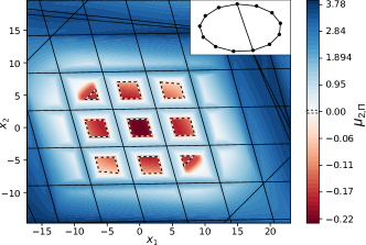
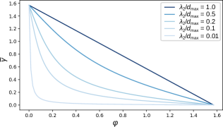
In Fig. 2, we illustrate to what extent the bound in Eq. (39) is conservative. The proximity of the boundary of the cohesive winding cell (dashed black line) and the area where the logarithmic seminorm turns positive (blue) confirms that our bound Eq. (39) is rather sharp. In other numerical experiments, we discovered that the condition in Theorem 3 is more conservative for denser network structures. We also illustrate this observation in Fig. 3, where we show the dependence of $\bar{\gamma}$ on both the frustration and the ratio between algebraic connectivity and maximal degree.

V At most uniqueness of synchronous states

Contracting systems over convex sets are known to have at most a unique equilibrium [16, Ex. 3.16]. Here we extend this property to the Kuramoto-Sakaguchi model by showing that the set over which it is semicontracting is actually convex.

Figure 3: Illustration of the upper bound $\bar{\gamma}$ of Theorem 3 as a function of the frustration $\varphi$, for various values of the ratio $\lambda_{2}/d_{\max}$. High values of $\lambda_{2}/d_{\max}$ typically correspond to densely connected graphs, confirming the intuition that such graphs tolerate less cohesive stable synchronous states, and vice-versa for low ratio $\lambda_{2}/d_{\max}$.

Theorem 4

Let $0<\gamma<\bar{\gamma}$, with $\bar{\gamma}$ defined in Eq. (39), and let $\bm{u}\in\mathbb{Z}^{c}$. Up to a constant phase shift and up to the addition of integer multiples of $2\pi$, there is at most one synchronous state of the Kuramoto-Sakaguchi model in the $\gamma$-cohesive $\bm{u}$-winding cell $\Gamma({\bm{u},\gamma})$.

Proof:

The proof of Theorem 4 leverages a natural polytopic representation (see Appendix -A) of each connected component of the $\gamma$-cohesive winding cell, presented in Ref. [22]. The polytopic representation of the winding cells conveniently allows the application of standard results of semicontraction theory, guaranteeing exponential convergence of the system. In summary, infinitesimal semicontractivity implies strong infinitesimal contractivity of a reduced system and the polytopic representation of the state space guarantees convexity of the contractive subdomain, implying at most uniqueness of the equilibrium therein. ∎

Theorem 4 improves previous at most uniqueness conditions [22, Theorem 4.1] and [23, Corollary 6] in that it applies to a wider class of models, has a less conservative condition on cohesiveness [Eq. (39)], and the condition for semicontractivity [Eq. (39)] is much more explicit than its counterpart in [23, Eq. (45)]. Furthermore, the proof is much more streamlined and elegant, which provides a clear insight on the underlying mechanisms leading to at most uniqueness, namely the local semicontractivity of the Kuramoto-Sakaguchi model. In Refs. [22, 23], the proof methods are ad hoc and tailored to the specific problem at hand.

VI Conclusion

Networks of Kuramoto-Sakaguchi oscillators gather all subtleties that need to be considered when applying semicontraction theory to a dynamical system. Due to rotational invariance, the Kuramoto-Sakaguchi model is not contracting, but at best semicontracting. Therefore, we first formulated the system in an appropriate framework, where semicontraction theory applies, and we defined the appropriate semicontraction metric, namely, the consensus seminorm. Furthermore, systems of Kuramoto-Sakaguchi oscillators are not semicontracting on the whole state space. Hence, we had to identify convex subdomains where semicontraction holds, which are the phase cohesive winding cells.

Tackling the question of synchronization in networks of Kuramoto-Sakaguchi oscillators through the prism of (semi)contraction shed light on the mechanisms leading to multistability. Moreover, contracting and semicontracting systems come with various convenient properties. In particular, resorting to semicontraction theory in our proof implies that it is robust against disturbances, noise, or unmodeled dynamics.

Also, contracting systems naturally come with associated Lyapunov functions [16, Eq. (3.28)]. Knowing these Lyapunov functions for the Kuramoto-Sakaguchi model opens new paths of investigation for open questions about networks of phase oscillators, such as the computation of attraction regions of synchronous states or the design of algorithms for the computation of fixed points.

-A Polytopic representation of the state space

It is shown in Ref. [22, Theorem 3.6] that for any $\bm{x}\in\Omega_{\Sigma}(\bm{u})$, there is a unique $\bm{y}\in\bm{1}_{n}^{\perp}$ such that

$$d_{\rm cc}(B^{\top}\bm{x}) =B^{\top}\bm{y}+2\pi C^{\dagger}_{\Sigma}\bm{u}\,,$$ (43)

where $B$ is the incidence matrix of the graph ${\cal G}$ and $C_{\Sigma}$ is the cycle-edge incidence matrix, defined, e.g., in [22, Eq. (2.1)]. Notice that even though the proof of [22, Theorem 3.6] is provided for points on the $n$-torus, the same proof directly extends to $\mathbb{R}^{n}$ through the natural construction of the $n$-torus as a quotient space of the Euclidean space.

The point $\bm{y}\in\bm{1}_{n}^{\perp}$ is easily reparametrized as $\bm{z}=R\bm{y}\in\mathbb{R}^{n-1}$, and one notices that $\bm{y}=R^{\dagger}\bm{z}$. By construction, $\bm{z}$ belongs to the polytope

$$P_{\bm{u}} =\left\{\bm{z}\in\mathbb{R}^{n-1}\colon\|B^{\top}R^{\dagger}\bm{z}+2\pi C_{\Sigma}^{\dagger}\bm{u}\|_{\infty}\leq\pi\right\}\,,$$ (44)

and we therefore have a natural projection

$$\begin{split}{\rm proj}_{\bm{u}}\colon\Omega_{\Sigma}(\bm{u})&\to P_{\bm{u}}\,.\end{split}$$ (45)

Furthermore, Ref. [22, Theorem 3.6] shows in particular that the projection is injective. Restricting the projection ${\rm proj}_{\bm{u}}$ to phase cohesive sets, one verifies that the $\gamma$-cohesive $\bm{u}$-winding cell, $\Gamma({\bm{u},\gamma})$, is injectively mapped to the $\gamma$-cohesive $\bm{u}$-polytope

$$P_{\bm{u},\gamma} =\left\{\bm{z}\in\mathbb{R}^{n-1}\colon\|B^{\top}R^{\dagger}\bm{z}+2\pi C_{\Sigma}^{\dagger}\bm{u}\|_{\infty}<\gamma\right\}\,,$$ (46)

which is convex by construction.

Let us see how the dynamics induced by the Kuramoto-Sakaguchi model [Eq. (1)] on $\bm{x}$ translates to the evolution of its image ${\rm proj}_{\bm{u}}(\bm{x})=\bm{z}\in P_{\bm{u}}$,

$$\dot{\bm{z}} =R(B^{\top})^{\dagger}B^{\top}R^{\dagger}\dot{\bm{z}}=R(B^{\top})^{\dagger}\frac{d}{dt}(B^{\top}R^{\dagger}\bm{z})$$

$$=R(B^{\top})^{\dagger}\frac{d}{dt}\left(d_{\rm cc}(B^{\top}\bm{x})-2\pi C_{\Sigma}^{\dagger}\bm{u}\right)\,.$$ (47)

Now, by definition of the counterclockwise difference, there exists $\bm{k}\in\mathbb{Z}^{m}$ such that $d_{\rm cc}(B^{\top}\bm{x})=B^{\top}\bm{x}+2\pi\bm{k}$. Furthermore, for almost all $\bm{x}$, the value of $\bm{k}$ is constant in a neighborhood of $B^{\top}\bm{x}$. Therefore, almost everywhere,

$$\dot{\bm{z}} =R(B^{\top})^{\dagger}\frac{d}{dt}\left(B^{\top}\bm{x}+2\pi\bm{k}-2\pi C_{\Sigma}^{\dagger}\bm{u}\right)$$

$$=R(B^{\top})^{\dagger}B^{\top}\dot{\bm{x}}=R\dot{\bm{x}}=Rf(\bm{x})\,,$$ (48)

where we used that $\bm{u}$ is constant. A posteriori, we verify that the above derivation does not depend on the choice of preimage $\bm{x}$ of $\bm{z}$. Indeed, two points $\bm{x}_{1},\bm{x}_{2}\in\Omega_{\Sigma}(\bm{u})$ that have the same image $\bm{z}\in P_{\bm{u}}$ satisfy $f(\bm{x}_{1})=f(\bm{x}_{2})$, and Eq. (-A) is valid everywhere.

The diffusive nature of the coupling functions $f_{i}$ implies that one can re-write them as functions of the pairwise component differences along the edges of the interaction graph. Namely, one can define $F_{i}\colon\mathbb{R}^{m}\to\mathbb{R}$ such that $f_{i}(\bm{x})=F_{i}(B^{\top}\bm{x})$. We then get

$$\dot{\bm{z}} =Rf(\bm{x})=RF(B^{\top}\bm{x})=RF(d_{\rm cc}(B^{\top}\bm{x}))$$

$$=RF(B^{\top}R^{\dagger}\bm{z}+2\pi C_{\Sigma}^{\dagger}\bm{u})=\tilde{f}(\bm{z})\,.$$ (49)

-B Proof the at most uniqueness (Theorem 4)

We first need to prove that the system Eq. (-A) is strongly infinitesimally contracting.

Lemma 5

Let $\bar{\gamma}$ as in Eq. (39), $0<\gamma<\bar{\gamma}$, and $\bm{u}\in\mathbb{Z}^{c}$. Then Eq. (-A) has at most a unique fixed point in $P_{\bm{u},\gamma}$.

Proof:

Using the chain rule and the property of pseudoinverses that $AA^{\dagger}A=A$, we compute the Jacobian of the system,

$$D\!{\tilde{f}}(\bm{z}) =R~{}D\!{F}(B^{\top}R^{\dagger}\bm{z}+2\pi C_{\Sigma}^{\dagger}\bm{u})B^{\top}R^{\dagger}$$

$$=R~{}D\!{F}(d_{\rm cc}(B^{\top}\bm{x}))B^{\top}(B^{\top})^{\dagger}B^{\top}R^{\dagger}$$

$$=R~{}D\!{F}(B^{\top}\bm{x})B^{\top}R^{\dagger}=RD\!{f}(\bm{x})R^{\dagger}\,,$$ (50)

independently of the choice for $\bm{x}$ the preimage of $\bm{z}$. Equation (-B) allows us to compute the logarithmic norm of the system $\dot{\bm{z}}=\tilde{f}(\bm{z})$,

$$\mu_{2}(D\!{\tilde{f}}(\bm{z})) =\mu_{2}(RD\!{f}(\bm{x})R^{\dagger})=\mu_{2,\Pi_{n}}(D\!{f}(\bm{x}))\,,$$ (51)

where we used Eq. (17), independently of the preimage $\bm{x}$.

For any point $\bm{z}\in P_{\bm{u},\gamma}$, any of its preimage $\bm{x}$ is $\gamma$-cohesive by definition. Therefore, by Eq. (51) and Theorem 3, the logarithmic norm of the system Eq. (-A) is strictly negative and the system is strongly infinitesimally contracting on $P_{\bm{u},\gamma}$.

Furthermore, by definition, the phase cohesive polytope $P_{\bm{u},\gamma}$ is convex. In summary, the system $\dot{\bm{z}}=\tilde{f}(\bm{z})$ is strongly infinitesimally contracting on a convex set. Note that $P_{\bm{u},\gamma}$ is not necessarily forward invariant. Therefore, by [16, Ex. 3.16], there is at most a unique fixed point in $P_{\bm{u},\gamma}$. ∎

We are now ready to prove Theorem 4. Let ${\bm{x}}^{\rm s}\in\Gamma({\bm{u},\gamma})$ be a synchronous state of Eq. (1), i.e., $f({\bm{x}}^{\rm s})=\omega^{\rm s}\bm{1}_{n}$. One can verify that $\bm{z}^{\rm s}={\rm proj}_{\bm{u}}(\bm{x}^{\rm s})\in P_{\bm{u},\gamma}$ is a fixed point of Eq. (-A), i.e., $\tilde{f}(\bm{z}^{\rm s})=0$. Therefore, if $\bm{x}^{\rm t}\in\Gamma({\bm{u},\gamma})$ is also a synchronous state of Eq. (1), then ${\rm proj}_{\bm{u}}({\bm{x}}^{\rm t})\in P_{\bm{u},\gamma}$ is also a fixed point of Eq. (-A) and Lemma 5 directly implies that ${\rm proj}_{\bm{u}}({\bm{x}}^{\rm t})=\bm{z}^{\rm s}$.

The projection ${\rm proj}_{\bm{u}}$ is such that $d_{\rm cc}(B^{\top}{\bm{x}}^{\rm s})=d_{\rm cc}(B^{\top}{\bm{x}}^{\rm t})$, i.e., $B^{\top}({\bm{x}}^{\rm s}-{\bm{x}}^{\rm t})=2\pi\bm{k}$, for some $\bm{k}\in\mathbb{Z}^{m}$. The graph ${\cal G}$ being connected, we can recursively reconstruct the vector of differences ${\bm{x}}^{\rm s}-{\bm{x}}^{\rm t}$ up to a constant shift. We conclude that for each node $i$, the difference $({\bm{x}}^{\rm s}-{\bm{x}}^{\rm t})_{i}$ is of the form $({\bm{x}}^{\rm s}-{\bm{x}}^{\rm t})_{i}=\rho+2\pi\ell_{i}$, with $\ell_{i}\in\mathbb{Z}$, where we do not know $\rho\in\mathbb{R}$, but it does not matter. Up to a constant shift $\rho$ of all components and up to an integer multiple of $2\pi$, ${\bm{x}}^{\rm s}$ and ${\bm{x}}^{\rm t}$ are then the same synchronous state, which concludes the proof.

References

- [1] S. H. Strogatz, Sync: The Emerging Science of Spontaneous Order, ser. Penguin Press Science Series. Penguin Adult, 2004.
- [2] C. Huygens, Oeuvres complètes de Christiaan Huygens, M. Nijhoff, Ed. Société hollandaise des sciences, 1993.
- [3] A. T. Winfree, “Biological rhythms and the behavior of populations of coupled oscillators,” J. of Theoretical Biology, vol. 16, no. 1, pp. 15–42, 1967.
- [4] Y. Kuramoto, “Cooperative dynamics of oscillator community a study based on lattice of rings,” Progress of Theoretical Physics Suppl., vol. 79, pp. 223–240, 1984.
- [5] H. Sakaguchi, S. Shinomoto, and Y. Kuramoto, “Mutual entrainment in oscillator lattices with nonvariational type interaction,” Progress of Theoretical Physics, vol. 79, no. 5, pp. 1069–1079, 1988.
- [6] A. Arenas, A. Díaz-Guilera, J. Kurths, Y. Moreno, and C. Zhou, “Synchronization in complex networks,” Physics Reports, vol. 469, no. 3, pp. 93–153, 2008.
- [7] S. Ling, R. Xu, and A. S. Bandeira, “On the Landscape of Synchronization Networks: A Perspective from Nonconvex Optimization,” SIAM J. on Optimization, vol. 29, no. 3, pp. 1879–1907, 2019.
- [8] J. C. Bronski, T. Carty, and L. DeVille, “Configurational stability for the Kuramoto-Sakaguchi model,” Chaos, vol. 28, p. 103109, 2018.
- [9] C. Balestra, F. Kaiser, D. Manik, and D. Witthaut, “Multistability in lossy power grids and oscillator networks,” Chaos, vol. 29, p. 123119, 2019.
- [10] W. Wang and J.-J. E. Slotine, “On partial contraction analysis for coupled nonlinear oscillators,” Biological Cybernetics, vol. 92, no. 1, pp. 38–53, 2005.
- [11] W. Lohmiller and J.-J. E. Slotine, “On contraction analysis for non-linear systems,” Automatica, vol. 34, no. 6, pp. 683–696, 1998.
- [12] S. Coogan, “A contractive approach to separable Lyapunov functions for monotone systems,” Automatica, vol. 106, pp. 349–357, 2019.
- [13] H. Tsukamoto, S.-J. Chung, and J.-J. E. Slotine, “Contraction theory for nonlinear stability analysis and learning-based control: A tutorial overview,” Annual Reviews in Control, vol. 52, pp. 135–169, 2021.
- [14] N. Boffi, S. Tu, N. Matni, J.-J. E. Slotine, and V. Sindhwani, “Learning stability certificates from data,” in Conf. on Robot Learning, ser. Proceedings of Machine Learning Research, J. Kober, F. Ramos, and C. Tomlin, Eds., vol. 155. PMLR, 16–18 Nov 2021, pp. 1341–1350. [Online]. Available: https://proceedings.mlr.press/v155/boffi21a.html
- [15] Z. Aminzare and E. D. Sontag, “Contraction methods for nonlinear systems: A brief introduction and some open problems,” in IEEE Conf. on Decision and Control, Dec. 2014, pp. 3835–3847.
- [16] F. Bullo, Contraction Theory for Dynamical Systems, 1.1 ed. Kindle Direct Publishing, 2023. [Online]. Available: https://fbullo.github.io/ctds
- [17] I. R. Manchester and J.-J. E. Slotine, “Transverse contraction criteria for existence, stability, and robustness of a limit cycle,” Systems & Control Letters, vol. 63, pp. 32–38, 2014.
- [18] F. Forni and R. Sepulchre, “A differential Lyapunov framework for contraction analysis,” IEEE Transactions on Automatic Control, vol. 59, no. 3, pp. 614–628, 2014.
- [19] C. Wu, I. Kanevskiy, and M. Margaliot, “-contraction: Theory and applications,” Automatica, vol. 136, p. 110048, 2022.
- [20] S. Jafarpour, P. Cisneros-Velarde, and F. Bullo, “Weak and Semi-Contraction for Network Systems and Diffusively Coupled Oscillators,” IEEE Transactions on Automatic Control, vol. 67, no. 3, pp. 1285–1300, 2022.
- [21] G. De Pasquale, K. D. Smith, F. Bullo, and M. E. Valcher, “Dual seminorms, ergodic coefficients and semicontraction theory,” submitted to IEEE TAC (arXiv preprint: 2201.03103), 2023.
- [22] S. Jafarpour, E. Y. Huang, K. D. Smith, and F. Bullo, “Flow and elastic networks on the -torus: Geometry, analysis, and computation,” SIAM Review, vol. 64, no. 1, pp. 59–104, 2022.
- [23] R. Delabays, S. Jafarpour, and F. Bullo, “Multistability and anomalies in oscillator models of lossy power grids,” Nature Communications, vol. 13, no. 1, p. 5238, 2022.
- [24] M. Fiedler, “Algebraic connectivity of graphs,” Czechoslovak Mathematical J., vol. 23, no. 2, pp. 298–305, 1973.
- [25] R. A. Horn and C. R. Johnson, Matrix Analysis. New York: Cambridge University Press, 1994.