On the momentum diffusion over multiphase surfaces with meshless methods

Abstract

This work investigates the effects of the choice of momentum diffusion operator on the evolution of multiphase fluid systems resolved with Meshless Lagrangian Methods (MLM). Specifically, the effects of a non-zero viscosity gradient at multiphase interfaces are explored. This work shows that both the typical Smoothed Particle Hydrodynamics (SPH) and Generalized Finite Difference (GFD) diffusion operators under-predict the shear divergence at multiphase interfaces. Furthermore, it was shown that larger viscosity ratios increase the significance of this behavior. A multiphase GFD scheme is proposed that makes use of a computationally efficient diffusion operator that accounts for the effects arising from the jump discontinuity in viscosity. This scheme is used to simulate a 3D bubble submerged in a heavier fluid with a density ratio of $2:1$ and a dynamic viscosity ratio of $100:1$. When comparing the effects of momentum diffusion operators, a discrepancy of 57.2% was observed in the bubble’s ascent velocity.

wcshort=WC, long=weakly compressible icshort=IC, long=incompressible ftshort=FT, long=front tracking fdshort=FD, long=finite difference mlmshort=MLM, long=meshless Lagrangian method gfdshort=GFD, long=generalized finite difference sphshort=SPH, long=smoothed particle hydrodynamics mpsshort=MPS, long=moving particle semi-implicit nseshort=NSE, long=Navier-Stokes equations pdeshort=PDE, long=partial differential equation demshort=DEM, long=discrete element method ppeshort=PPE, long=pressure Poisson equation gpushort=GPU, long=graphics processing unit lesshort=LES, long=large eddy simulation evmshort=EVM, long=eddy viscosity model csfshort=CSF, long=continuous surface force fvmshort=FVM, long=finite volume method rmseshort=RMSE, long=root mean squared error bicgshort=BiCGSTAB, long=bi-conjugate gradient stabilized

1 Introduction

The prediction of multiphase flow phenomena is a widespread problem in various physical and engineering environments with applications in fields such as oil and gas production, power generation, and chemical processing. Recently, mlm have become a popular alternative to mesh-based approaches for simulating multiphase flow due to them avoiding many of the challenges introduced when considering the fluids from an Eulerian perspective, especially when considering interface tracking. mlm discretize the domain with a point cloud that is free to evolve. These points, often referred to as fluid “particles” carry fluid information with them. This allows the fluid to be evaluated from a Lagrangian perspective, and thus allows advection to be handled implicitly by updating fluid particle positions appropriately. In a multiphase flow context, this provides a natural framework for treating interface advection in a manner that solely depends on tracking the initial phase assigned to a particle.

It is common for multiphase mlm schemes to adapt multiphase models originally proposed for mesh-based schemes. One of the most popular multiphase models for mlm remains the color function-based approach first introduced by Brackbill et al. [1]. This work proposed a scalar field that can be used to distinguish between phases and resolve interfaces, surface normals, and surface tension forces. The surface normal and surface tension are resolved using the gradient of the color function. In an Eulerian context, this field evolves via fluid advection, however, from a Lagrangian perspective, the color function is a constant particle-level property. This makes introducing the color function trivial for Lagrangian frameworks and, as a result, has seen extensive use in various mlm schemes including wc sph [2, 3], ic sph [4, 5, 6] and both wc [7] and ic [8] mps method. With mlm primarily categorized by their discretization of differential operators, the choice of scheme influences the resolution of the color gradient. To improve the accuracy of the interface resolution, higher-order gradient schemes are often used to resolve the gradients [3, 9, 10, 11], despite these differential operators being more computationally expensive to evaluate.

When resolving momentum diffusion operators, sph schemes typically utilize operators based on a hybrid sph-fd Laplacian operators of Morris et al. [12] or the artificial viscosity-based diffusion operator originally proposed by Monaghan and Gingold [13] as a stabilizing method. Hu et al. [2] proposed a modified Morris-style diffusion operator in the context of multiphase flow by basing the hybrid sph-fd approximation on the form of the sph pressure gradient form rather than the velocity gradient. Although both Monaghan and Morris-style diffusion operators have become popular choices for multiphase flow applications, as highlighted in [14], Morris-style diffusion operators are preferred since they can better handle the deformation and splitting of the multiphase interfaces.

While both models allow for variations in viscosity, neither resolve viscosity sensitivities nor account for the associated momentum diffusion [15]. Although the sensitivities are zero for fluids with constant fluid properties, a discontinuity in viscosity arises across interfaces with different material properties. As a result, although momentum far from the interface is diffused appropriately, the surface shear at the interface is only partially recovered by these momentum diffusion models. Despite this, these momentum diffusion operators remain the most common choice for multiphase sph schemes, even in modern work [9, 15, 16, 17, 11].

As an alternative to sph, the gfd method [18, 19, 20] offers an alternative way of constructing an mlm scheme by building the required differential operators from weighted Taylor-series expansions directly. The differential operator approximations are of a higher order than classical sph and are more computationally efficient to compute than the equivalent gradient-correct sph operators [21], but, as with gradient-corrected sph, this comes at a relaxation of the physical symmetries strongly enforced by classical sph. Regardless, gfd has been used to simulate both ic [22] and wc [21] fluids and have also shown to be well-suited for multi-physics applications [23].

This work systematically explores and compares different mlm diffusion models to quantify the effect of the viscosity sensitivity on the recovered solutions. First, the responses of the diffusion operators applied to static fields are compared. Next, to investigate the effect of sharp viscosity transitions on the mlm operators, the diffusion operators are applied to a steady-state multiphase flow solution. Finally, a direct comparison between full 3D simulations of a bubble rising in a fluid is performed. Comparisons between gfd and sph momentum diffusion operators are performed on static fields, but in the interest of limiting the computational requirements of this study, the full 3D simulation only considers the gfd diffusion operators. As part of this paper’s output, a computationally inexpensive viscosity gradient is proposed.

2 Numerical methods

This work is considered in the context of incompressible multiphase flow and as such the governing equations of motion are given by the incompressible nse:

$$\nabla\cdot\mathbf{u} =0,$$ (1)

$$\rho\frac{d\mathbf{u}}{dt} =-\nabla p+\nabla\cdot\mathbf{\tau}+\rho\mathbf{g}+\mathbf{S},$$ (2)

with $\mathbf{u}$ the velocity, $\rho$ the density, $p$ the pressure, $\rho\mathbf{g}$ the external body force, $\mathbf{S}$ the interface surface tension force as discussed in Section 2.2 and $\mathbf{\tau}=2\mu\mathbf{T}$ a Newtonian shear stress tensor with $\mu$ the dynamic viscosity and:

$$\mathbf{T}=\frac{1}{2}\left[\nabla\otimes\mathbf{u}+(\nabla\otimes\mathbf{u})^{T}\right],$$ (3)

the symmetric strain rate tensor for incompressible flow.

It should be noted that (2) makes use of the total time derivative due to the Lagrangian nature of mlm automatically treating advection by updating particle positions. Furthermore, no additional work is needed to track surface interfaces as the interface update is directly obtained from the updated fluid particle positions.

Although all material properties are kept constant in this work, both density and especially dynamic viscosity are allowed to vary between fluids, leading to discontinuities in the density and viscosity fields at fluid interfaces. As such, a major focus of this work is set on the diffusion operator at the fluid interfaces where the viscosity gradient is non-zero.

2.1 Meshless operators

Although mlm differential operator approximations stem from various different contexts, the connectivity between points in these meshless schemes generally follows a kernel weighting approach allowing point-wise information to locally diffuse in its neighboring area. This work uses a quintic kernel [12]:

$$W(\mathbf{r},h)=w_{0}\begin{cases}(3-q)^{5}-6(2-q)^{5}+15(1-q)^{5}&\text{for $0\leq q\leq 1$}\\ (3-q)^{5}-6(2-q)^{5}&\text{for $1<q\leq 2$}\\ (3-q)^{5}&\text{for $2<q\leq 3$}\\ 0&\text{otherwise}\end{cases}\qquad\text{with}\qquad q={\lVert}\mathbf{r}{\rVert}/h,$$ (4)

with $\mathbf{r}$ a position vector, $3h$ the support radius, $w_{0}$ a normalization constant and $\lVert\cdot\rVert$ indicating the Euclidean norm. For sph operators in 2D, $w_{0}=7/478\pi$. As a renormalized scheme, gfd operators do not require a normalized kernel and so set $w_{0}=1$. A finite support radius is used to limit particle interaction to only its local neighborhood. The notation $W_{ij}=W(\mathbf{r}_{i}-\mathbf{r}_{j},h)$ is used to indicate the kernel weighting between particles $i$ and $j$. Furthermore, this notion is extended to general fields as well using $f_{i}=f(\mathbf{r}_{i})$ to indicate the function value of the field $f$ at the $i^{th}$ particle’s position. Finally, $\mathbf{r}_{ij}=\mathbf{r}_{i}-\mathbf{r}_{j}$ is used to indicates the position of the $i^{th}$ particle relative to the $j^{th}$ particle.

As proposed by Zainali et al. [6], jump discontinuities in material properties are smoothed by applying a Shepard filter [24]:

$$\widetilde{f}_{i}=\frac{\sum_{j\in I}f_{j}W_{ij}}{\sum_{j\in I}W_{ij}},$$ (5)

with $f$ either density or viscosity, $I=\left\{j\in\mathbb{Z}/N\mathbb{Z}:W_{ij}>0\right\}$ the indexing set of the $i^{th}$ particle’s neighbors and $\widetilde{\left(\cdot\right)}$ indicating a filtered property.

As required by the multiphase model, the so-called color function $C^{n}$ is introduced as:

$$C^{n}_{i}=\frac{\sum_{j\in I^{n}}W_{ij}}{\sum_{j\in I}W_{ij}},$$ (6)

with $I^{n}$ the indexing set of all nodes in the support radius of $i^{th}$ particle and in the $n^{th}$ phase. Since each phase’s material properties are constant and with only two phases considered in this work, all filtered fields can be resolved based on one of the color functions:

$$\widetilde{f}_{i}=f^{0}C_{i}^{0}+f^{1}C_{i}^{1}=f^{1}+(f^{0}-f^{1})C_{i}^{0},$$ (7)

with $f^{0}$ and $f^{1}$ the relevant material properties of the first and second phases, respectively.

The remainder of this section is dedicated to the gfd and sph differential operators. It should be mentioned that a full sph scheme is not considered in this work, and so only the momentum diffusion operator is discussed. Although both gfd gradients and Laplacians are discussed in detail, this section also mainly focuses on the construction of the momentum diffusion operator.

2.1.1 GFD differential operators

At a high level, the gfd method constructs meshless differential operators by kernel weighting finite-difference terms constructed from Taylor-series approximations. The gfd differential operators used in this work are based on the gradient approximation of Lanson and Vila [18, 19] and the Laplacian approximation of Basic et al. [20]. For a general field $f$ over a $d$-dimensional Euclidean space at the $i^{th}$ particle, these approximations are given by:

$$\left<\nabla f\right>_{i} =\mathbf{B}_{i}\cdot\sum_{j\in I}(f_{i}-f_{j})W_{ij}\mathbf{r}_{ij},$$ (8)

$$\left<\nabla^{2}f\right>_{i} =2d\frac{\sum_{j\in I}(f_{j}-f_{i})W_{ij}\left(1-\mathbf{r}_{ij}\cdot\mathbf{o}_{i}\right)}{\sum_{j\in I}\lVert\mathbf{r}_{ij}\rVert^{2}W_{ij}\left(1-\mathbf{r}_{ij}\cdot\mathbf{o}_{i}\right)},$$ (9)

With:

$$\mathbf{B}_{i} =\left(\sum_{j\in I}W_{ij}\mathbf{r}_{ij}\otimes\mathbf{r}_{ij}\right)^{-1},$$ (10)

$$\mathbf{o}_{i} =\mathbf{B}_{i}\cdot\sum_{j\in I}W_{ij}\mathbf{r}_{ij},$$ (11)

the truncation tensor and offset vector, respectively. While this does not account for all differential operators of the nse, the forcing condition (2) can be constructed using these differential operators. Specifically, the momentum diffusion operator $\nabla\cdot\mathbf{\tau}$ can be decomposed as $\nabla\mu\cdot(2\mathbf{T})+\mu\nabla^{2}\mathbf{u}$. Clearly, this form only requires gradient and Laplacian approximations.

sph diffusion operators typically build viscosity smoothing into their differential operators. To allow for a more direct comparison, a gfd diffusion operator following a similar approach is introduced:

$$\left<\mu\nabla^{2}\mathbf{u}\right>_{i}=2d\frac{\sum_{j\in I}\left(\frac{2\widetilde{\mu}_{i}\widetilde{\mu}_{j}}{\widetilde{\mu}_{i}+\widetilde{\mu}_{j}}\right)(\mathbf{u}_{i}-\mathbf{u}_{j})W_{ij}\left(1-\mathbf{r}_{ij}\cdot\mathbf{o}_{i}\right)}{\sum_{j\in I}\lVert\mathbf{r}_{ij}\rVert^{2}W_{ij}\left(1-\mathbf{r}_{ij}\cdot\mathbf{o}_{i}\right)}.$$ (12)

There is no appreciable difference in computational cost between the gfd approximation $\left<\mu\nabla^{2}\mathbf{u}\right>$ and $\mu\left<\nabla^{2}\mathbf{u}\right>$. As such, the increased computational cost of utilizing the full shear stress divergence $\left<\frac{\nabla\cdot\mathbf{\tau}}{\rho}\right>$ is primarily due to its dependency on $\left<\frac{\nabla\mu}{\rho}\right>$ and $\left<\nabla\otimes\mathbf{u}\right>$.

2.1.2 SPH diffusion operator

Unlike gfd operators, the sph differential operators are based on the analytical derivative of the continuous fields constructed from a kernel-weighting process. As such, rather than building differential operators from weighted finite difference terms, sph differential operators are based on the kernel gradient $\nabla_{i}W_{ij}=\frac{\partial W_{ij}}{\partial\mathbf{r}_{i}}$.

Although this is typically suitable for gradient approximations, second-order differential approximations built from analytical second-order kernel derivatives are generally poor due to a strong sensitivity to particle disorder with certain particle configurations even leading to non-physical diffusion. For this reason, sph diffusion operators typically make use of a hybrid sph-fd approach.

In the context of multiphase flow, the momentum diffusion operator plays an important role in the evolution of the multiphase interface. As shown in [14], the Morris-style diffusion operator of [2] is more suitable compared to Monaghan-style operators since it allows for more accurate interface deformation with sharper interfaces. For this reason, the diffusion operator of [2] as presented in [14] will be used in this work:

$$\left<\mu\nabla^{2}\mathbf{u}\right>_{i}=\frac{1}{V_{i}}\sum_{j\in I}\left(\frac{2\widetilde{\mu}_{i}\widetilde{\mu}_{j}}{\widetilde{\mu}_{i}+\widetilde{\mu}_{j}}\right)\left(V_{i}^{2}+V_{j}^{2}\right)\left(\mathbf{u}_{i}-\mathbf{u}_{j}\right)\frac{\mathbf{r}_{ij}\cdot\nabla_{i}W_{ij}}{\lVert\mathbf{r}_{ij}\rVert^{2}},$$ (13)

with $V_{i}$ and $V_{j}$ the volume of the $i^{th}$ and $j^{th}$ fluid particle. It should be noted that the traditional correction for singular values in the denominator is omitted since the definition of $I$ ignores cases with particle distances equal to 0.

It should be noted that, unlike the gfd operators, the sph operators do not apply any kernel corrections. As such, not only is the order of the approximations lower, but it also significantly suffers from reduced kernel support at surfaces. For this reason, additional boundary particles are generated outside the computational domain for all comparisons between gfd and sph.

2.2 Multiphase flow

As highlighted in (2), multiphase physics requires the resolution of a surface tension forcing $\mathbf{S}$ at fluid interfaces. The surface tension model first proposed by Brackbill et al. [1] in a fvm context has been adapted for mlm. More specifically, the gradient of $C^{0}$ is used to identify surface interfaces and resolve the surface normal.

The normal direction $\mathbf{N}_{i}$ is determined as:

$$\mathbf{N}_{i}=\left<\frac{\nabla C^{0}}{\rho}\right>_{i}=\mathbf{B}_{i}\cdot\sum_{j\in I}\frac{C_{i}^{0}-C_{j}^{0}}{\bar{\rho}_{ij}}W_{ij}\mathbf{r}_{ij}$$ (14)

with $\bar{\rho}_{ij}=\frac{1}{2}(\widetilde{\rho}_{i}+\widetilde{\rho}_{j})$ the average density.

Following a modified implementation of the scheme proposed by Yang et al. [25], interface particles are identified by filtering the color gradient magnitude. As such, the normal is resolved as:

$$\hat{\mathbf{n}}_{i}=\begin{cases}\frac{\mathbf{N}_{i}}{\lVert\mathbf{N}_{i}\rVert}&\text{if}\quad\widetilde{\rho}_{i}\lVert\mathbf{N}_{i}\rVert>\epsilon/h\\ 0&\text{otherwise}\end{cases}$$ (15)

with $\epsilon$ a user-specified parameter to control the aggressiveness of the filter. It was found that $\epsilon=0.01$ was suitable for all simulations in this work.

The surface curvature $\kappa$ is obtained from the divergence of the surface normal:

$$\kappa_{i}=-\left<\nabla\cdot\hat{\mathbf{n}}\right>_{i}=\sum_{j\in I\cap I^{m}}W_{ij}\left(\hat{\mathbf{n}}_{j}-\hat{\mathbf{n}}_{i}\right)\cdot\mathbf{B}_{i}\cdot\mathbf{r}_{ij}$$ (16)

with $I^{m}=\left\{j\in\mathbb{Z}/N\mathbb{Z}:\lVert\mathbf{n}_{j}\rVert>0\right\}$ the indexing set of all particles bypassing the filter. This ensures that only particles on the interface contribute to this approximation.

The acceleration due to surface tension force $\mathbf{s}=\mathbf{S}/\rho$ is then resolved as:

$$\left<\mathbf{s}\right>_{i}=-\sigma\left<\nabla\cdot\hat{\mathbf{n}}\right>_{i}\left<\frac{\nabla C^{0}}{\rho}\right>_{i},$$ (17)

with $\sigma$ the surface tension coefficient. It should be noted that only particles indexed by $I^{m}$ have a non-zero $\left<\mathbf{s}\right>_{i}$.

Furthermore, the color gradient is reused when determining the viscosity gradient with effectively no additional computational cost required. By taking the gradient of (5) applied to the viscosity, then the viscosity gradient can be determined as:

$$\left<\frac{\nabla\mu}{\rho}\right>_{i}=(\mu^{0}-\mu^{1})\left<\frac{\nabla C^{0}}{\rho}\right>_{i}$$ (18)

with $\mu^{0}$ and $\mu^{1}$ indicating the dynamic viscosity of the first and second phases, respectively. It should be noted that since velocity is updated directly, the form of (18) is constructed for velocity diffusion rather than momentum diffusion. As such, the velocity diffusion operator is resolved as:

$$\left<\frac{\nabla\cdot\mathbf{\tau}}{\rho}\right>_{i}=\left<\frac{\nabla\mu}{\rho}\right>_{i}\cdot\left<2\mathbf{T}\right>_{i}+\widetilde{\nu}_{i}\left<\nabla^{2}\mathbf{u}\right>_{i},$$ (19)

with $\widetilde{\nu}_{i}=\widetilde{\mu}_{i}/\widetilde{\rho}_{i}$ the filtered kinematic viscosity.

2.3 Integration scheme

A projection method similar to incompressible sph and mps is used to enforce the incompressibility condition (1). An initial update step is used to introduce the viscous momentum diffusion, surface tension forces, and other body forces. This results in an unconstrained intermediate velocity field $\mathbf{u}^{*}$. A divergence-free velocity field is obtained by resolving the pressure such that the pressure gradient suppresses $\nabla\cdot\mathbf{u}^{*}$.

For the $k^{th}$ update step, the intermediate particle velocity is resolved as:

$$\mathbf{u}_{i}^{*}=\mathbf{u}_{i}^{k}+\Delta t\left(\left<\mathbf{L}\right>_{i}+\mathbf{g}_{i}+\left<\mathbf{s}\right>_{i}\right),$$ (20)

with $\Delta t$ the time-step size and $\left<\mathbf{L}\right>_{i}$ the appropriate velocity diffusion operator. The velocity field is then resolved via the projection step:

$$\mathbf{u}_{i}^{k+1}=\mathbf{u}_{i}^{*}-\Delta t\left<\frac{\nabla p^{k+1}}{\rho}\right>_{i}.$$ (21)

where $p^{k+1}$ is the pressure field that results in the divergence-free velocity and:

$$\left<\frac{\nabla p}{\rho}\right>_{i}=\mathbf{B}_{i}\cdot\sum_{j\in I}\frac{p_{i}-p_{j}}{\bar{\rho}_{ij}}W_{ij}\mathbf{r}_{ij}.$$ (22)

The system is closed by taking the divergence of (21), and setting $\nabla\cdot\mathbf{u}_{i}^{k+1}=0$ to obtain the ppe:

$$\left<\frac{\nabla^{2}p^{k+1}}{\rho}\right>_{i}=\frac{1}{\Delta t}\left<\nabla\cdot\mathbf{u}^{*}\right>_{i}.$$ (23)

Discretizing the ppe results in a sparse large linear system that is solved iteratively with a bicg method with a Jacobi pre-conditioner. The density field may become noisy when violent mixing takes place resulting in particles from one phase becoming surrounded by another. To introduce smoothing, the average density is used to scale each finite-difference term. As such, the pressure Laplacian of is resolved as:

$$\left<\frac{\nabla^{2}p^{k+1}}{\rho}\right>_{i}=2d\frac{\sum_{j\in I}\left(\frac{p_{j}-p_{i}}{\bar{\rho}_{ij}}\right)W_{ij}\left(1-\mathbf{r}_{ij}\cdot\mathbf{o}_{i}\right)}{\sum_{j\in I}\lVert\mathbf{r}_{ij}\rVert^{2}W_{ij}\left(1-\mathbf{r}_{ij}\cdot\mathbf{o}_{i}\right)}.$$ (24)

Again, since the material property is constant for individual phases, this approximation reduces to $\left<\nabla^{2}p\right>_{i}/\rho_{i}$ for any fluid particle far from the multiphase interface resulting in the typical single-phase incompressible gfd model.

The particle position is updated according to:

$$\mathbf{r}_{i}^{k+1}=\mathbf{r}_{i}^{k}+\frac{\Delta t}{2}\left(\mathbf{u}_{i}^{k}+\mathbf{u}_{i}^{k+1}\right)$$ (25)

Finally, to address clustering, the anti-clustering algorithm of Xu et al. [26] is used to shift the particles and create a more uniformly distributed particle collection.

3 Results

3.1 Verification study

In this section, the momentum diffusion operators of Section 2.1 are validated. The schemes are applied to Franke’s bivariate function [27]:

$$\begin{split}f(x,y)&=0.75\exp\left(-\frac{1}{4}(9x-2)^{2}-\frac{1}{4}(9y-2)^{2}\right)\\ &+0.75\exp\left(-\frac{1}{49}(9x+1)^{2}-\frac{1}{10}(9y+1)\right)\\ &+0.5\exp\left(-\frac{1}{4}(9x-7)^{2}-\frac{1}{4}(9y-3)^{2}\right)\\ &-0.2\exp\left(-(9x-4)^{2}-(9y-7)^{2}\right)\end{split}$$ (26)

Since the momentum diffusion operators will be applied to this field, a scalar field $\eta$ representing the dynamic viscosity is also required. As such, the approximations are compared against $\eta\nabla^{2}f$. First, a constant field $\eta=1$ is chosen to directly compare the analytical Laplacian and its meshless approximations.

The schemes are tested over both regularly and irregularly spaced points distributed over $\left\{\left.x,y\in\mathbb{R}^{2}\right|0\leq x\leq 1,0\leq y\leq 1\right\}$. The irregular configuration is generated by perturbing each point randomly in both $x$ and $y$ with distances sampled from a uniformly random distribution with a range of $[-c\delta_{0},c\delta_{0}]$ with $c$ a scale factor and $\delta_{0}$ the initial particle spacing. The support radius is given as $3h=(2.5+2c)\delta_{0}$. This accounts for the increase in particle distances due to shifting. All irregular grids in this work use $c=0.1$. Boundary effects are avoided by generating particles up to $3h$ outside the computational domain. The internal and boundary nodes for both the regular and irregular grids with $\delta_{0}=0.025$ can be seen in Figure 1(a) and Figure 1(b), respectively.

(a)

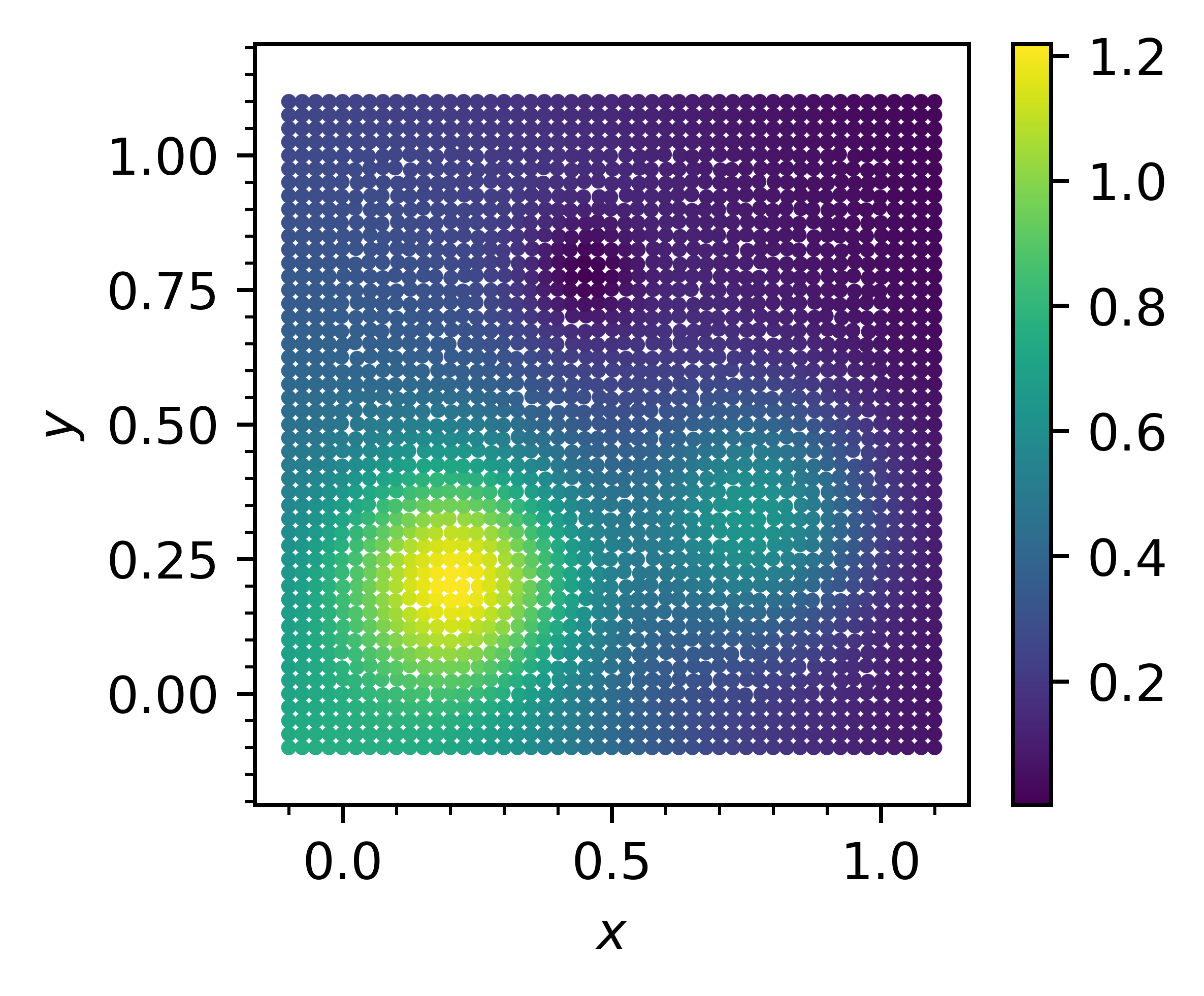
(b)

Figure 1: Particle configuration for the $41\times 41$ (a) regular grid and (b) irregular grid cases.

Figure 2 shows the absolute error of the gfd and sph Laplacian approximations applied to the regular configuration seen in Figure 1(a). Both the sph and gfd operators show similar qualitative behavior, with the largest errors present around the function peaks. Although the gfd operator has a lower error compared to the sph operator, the errors are in the same order of magnitude. Similarly, Figure 3 shows the results for the irregular configuration. Here it can be seen that the gfd errors still align well with the function peaks. Conversely, the sph errors are less dependent on function shape and primarily driven by the irregularity of the particle distribution. Compared to the regular grid results, although the gfd results are less accurate on the irregular grid, the operator still produces errors in the same order of magnitude. The sph operator suffers from a significant error increase when applied to an irregular grid.

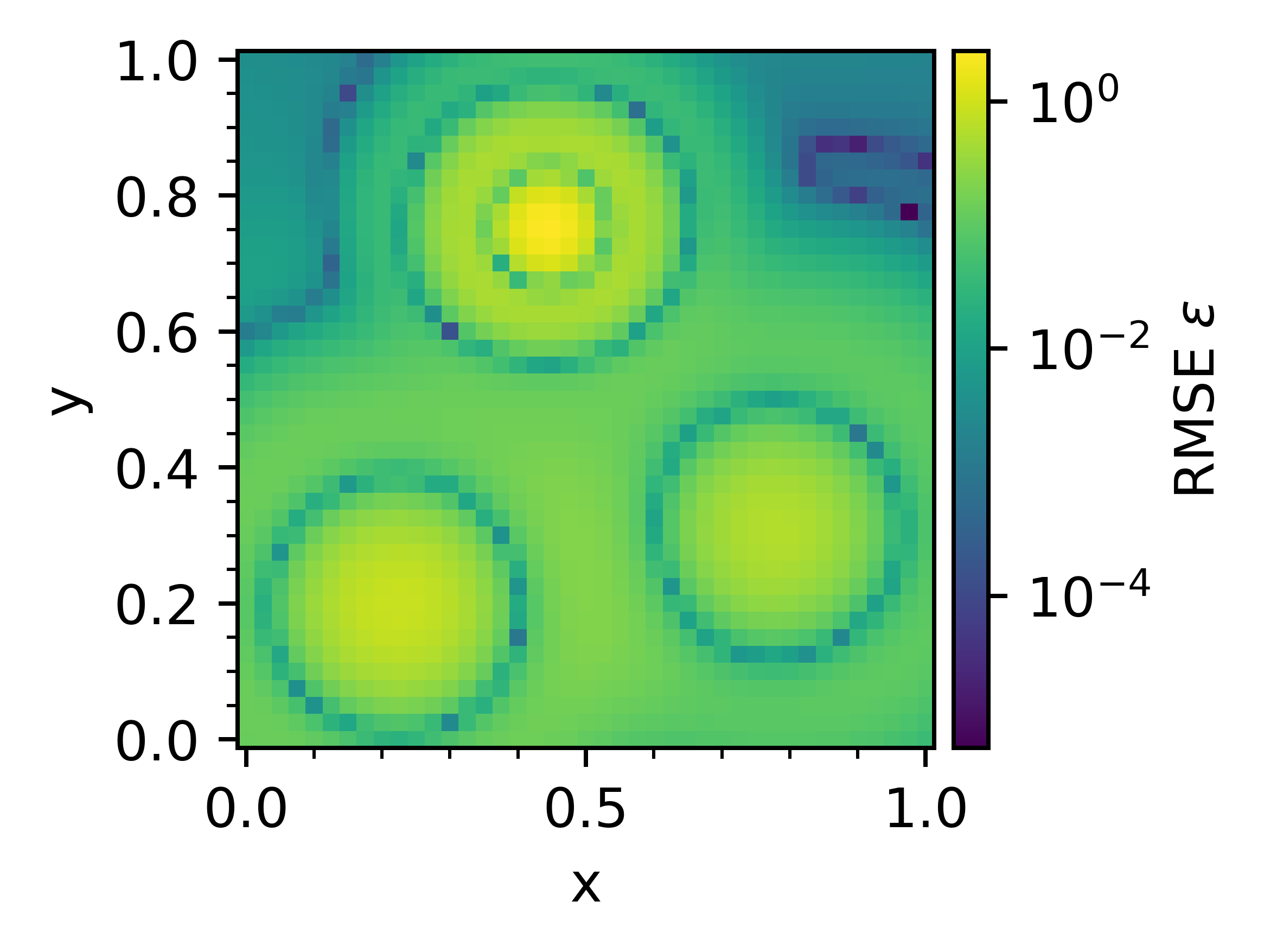
(a)

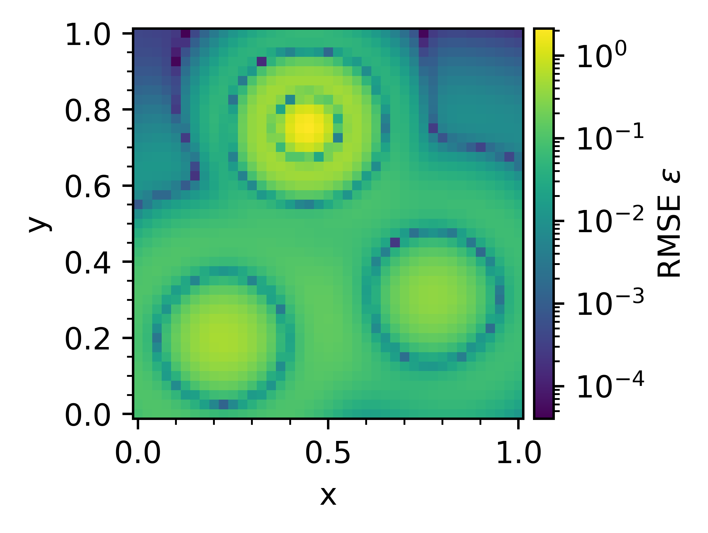
(b)

Figure 2: Particle level absolute error for the $41\times 41$ regular grid case for the (a) sph and (b) gfd diffusion operators.

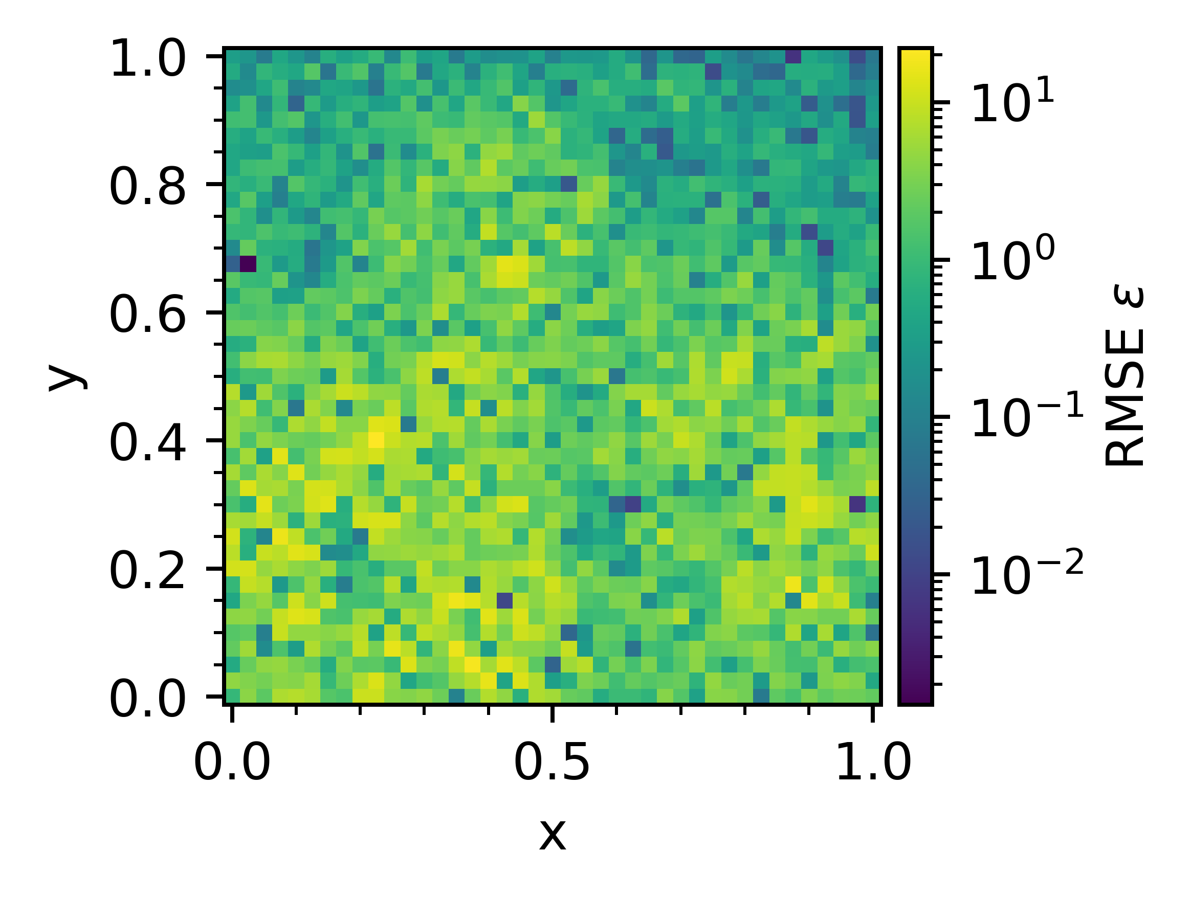
(a)

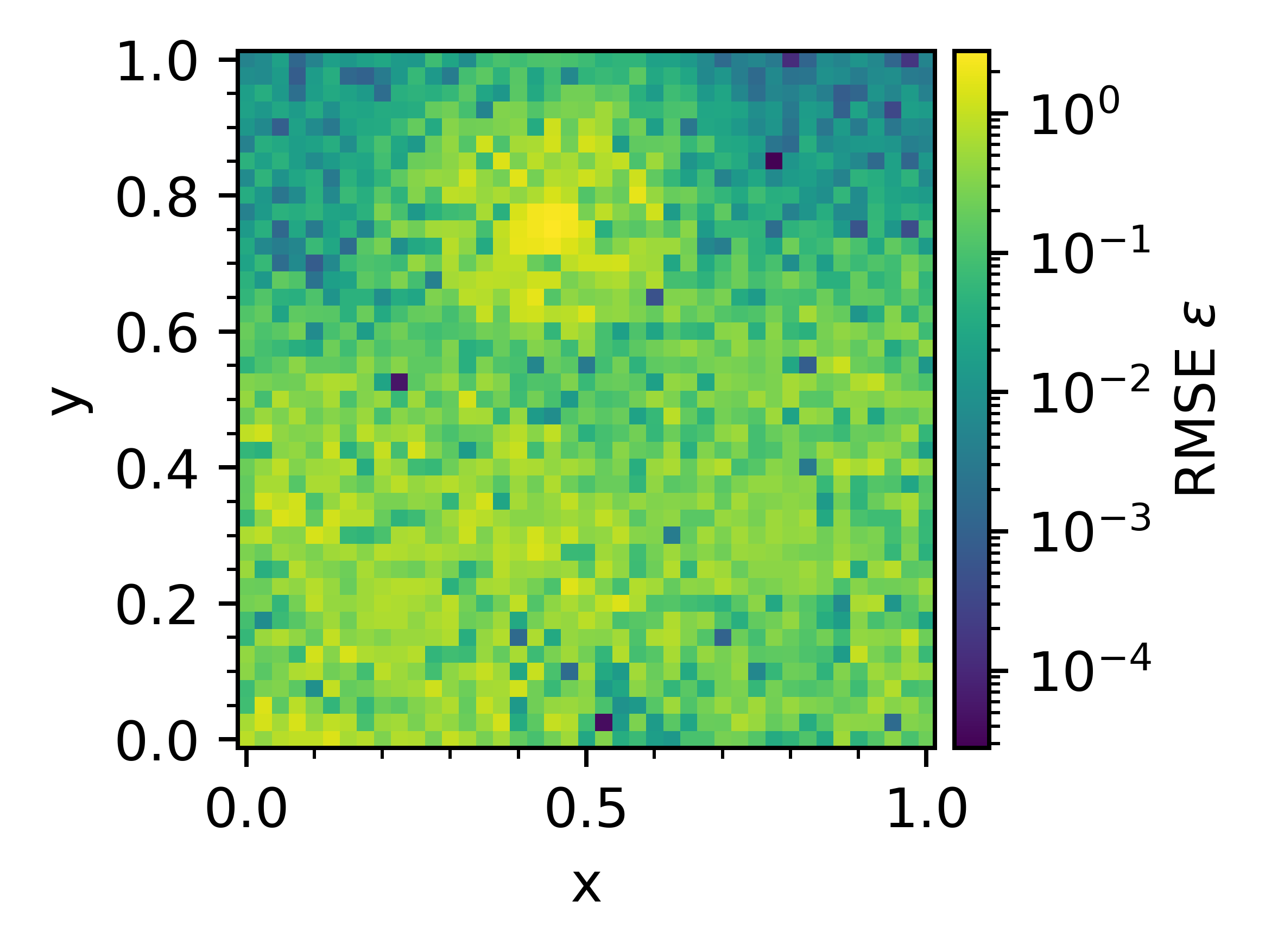
(b)

Figure 3: Particle level absolute error for the $41\times 41$ irregular grid case for the (a) sph and (b) gfd diffusion operators.

A convergence study for both the sph and gfd operators on a regular and irregular grid can be seen in Figure 4. The normalized rmse is defined as:

$$\epsilon=\frac{\sqrt{\sum_{i}\left[\left<L(f,\eta)\right>_{i}-\eta\nabla^{2}f(\mathbf{r}_{i})\right]^{2}}}{\sqrt{\sum_{i}\left[\eta\nabla^{2}f(\mathbf{r}_{i})\right]^{2}}}$$ (27)

with $\left<L(f,\eta)\right>_{i}$ a momentum diffusion operator. The rmse is plotted against particle size. For the regular spacing, both operators show similar accuracy initially, but the sph operator’s rate of convergence reduces as the number of particles increases while the gfd operator shows a consistent rate of convergence throughout the tested range. Irregularity can be seen to have a detrimental effect on both the sph and gfd error and rate of convergence. It can be seen that particle irregularity introduces a limit on the rmse of the gfd operator. Obtaining the same behavior observed in [20], the sph operator behaves especially poorly as it sees an increase in the rmse with an increase in the number of particles. This is due to sph resolving the Laplacian in an averaged sense. Regions with high irregularity resolve the Laplacian with large over- and under-predictions, leading to a large error at the particle level.

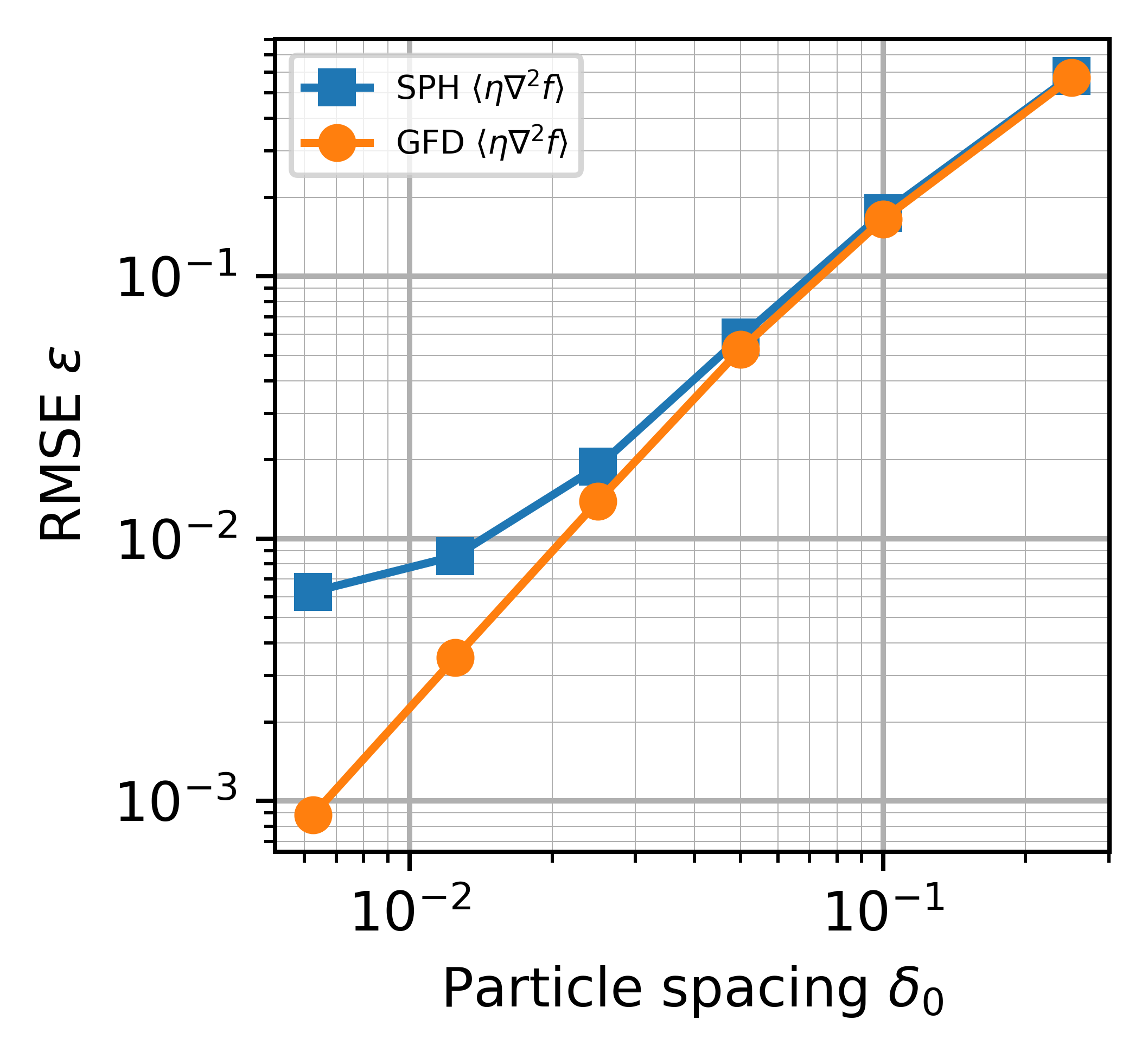
(a)

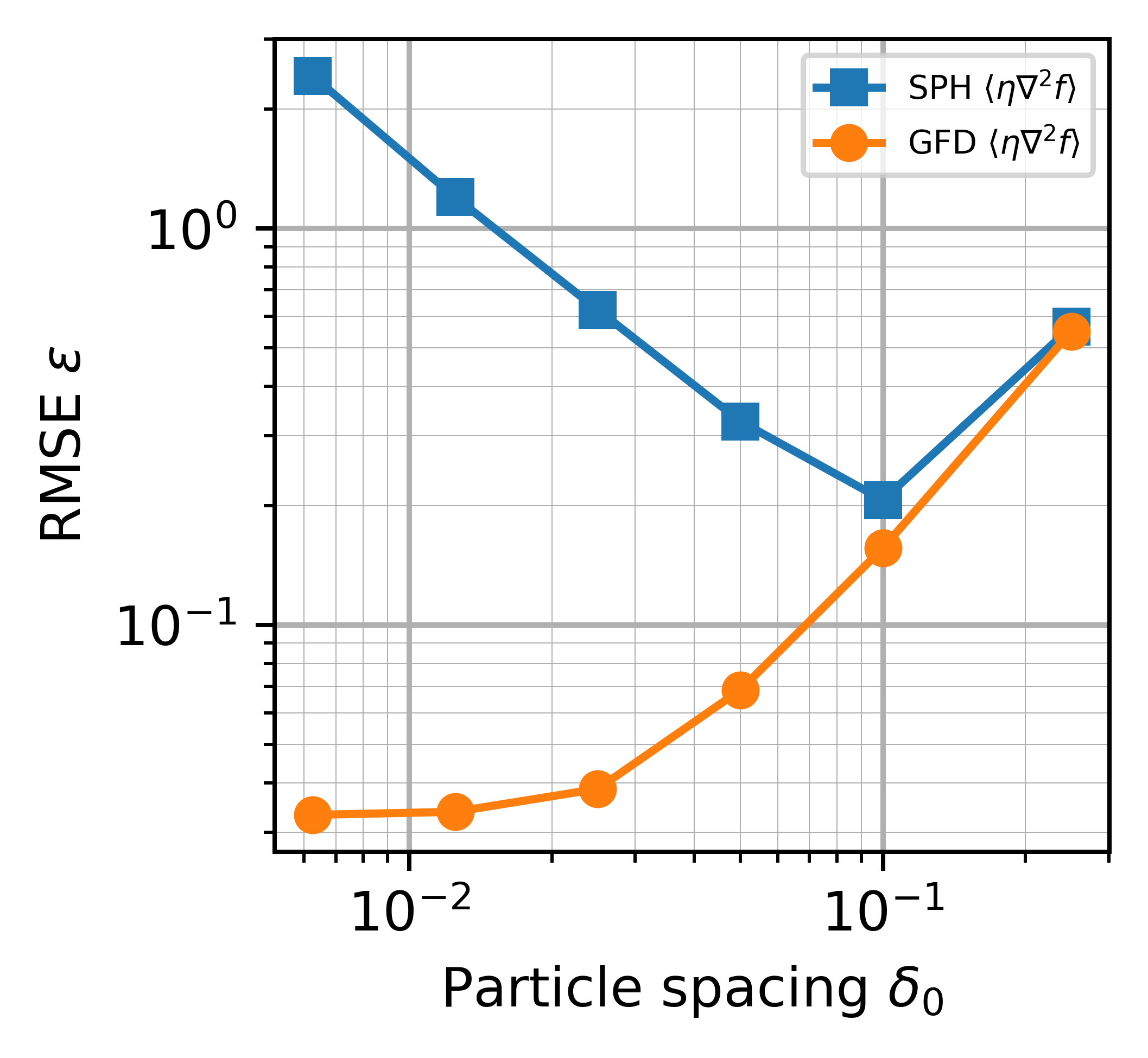
(b)

Figure 4: sph and gfd diffusion operators rmse on a (a) regular and (b) irregular grid.

Next, a convergence study is performed with a linearly-varying scale field given by $\eta(x,y)=1+x/2+y/2$. The results can be seen in Figure 5. Here, along with the sph operator, both $\left<\eta\nabla^{2}f\right>$ and $\eta\left<\nabla^{2}f\right>$ are resolved using the gfd operator.

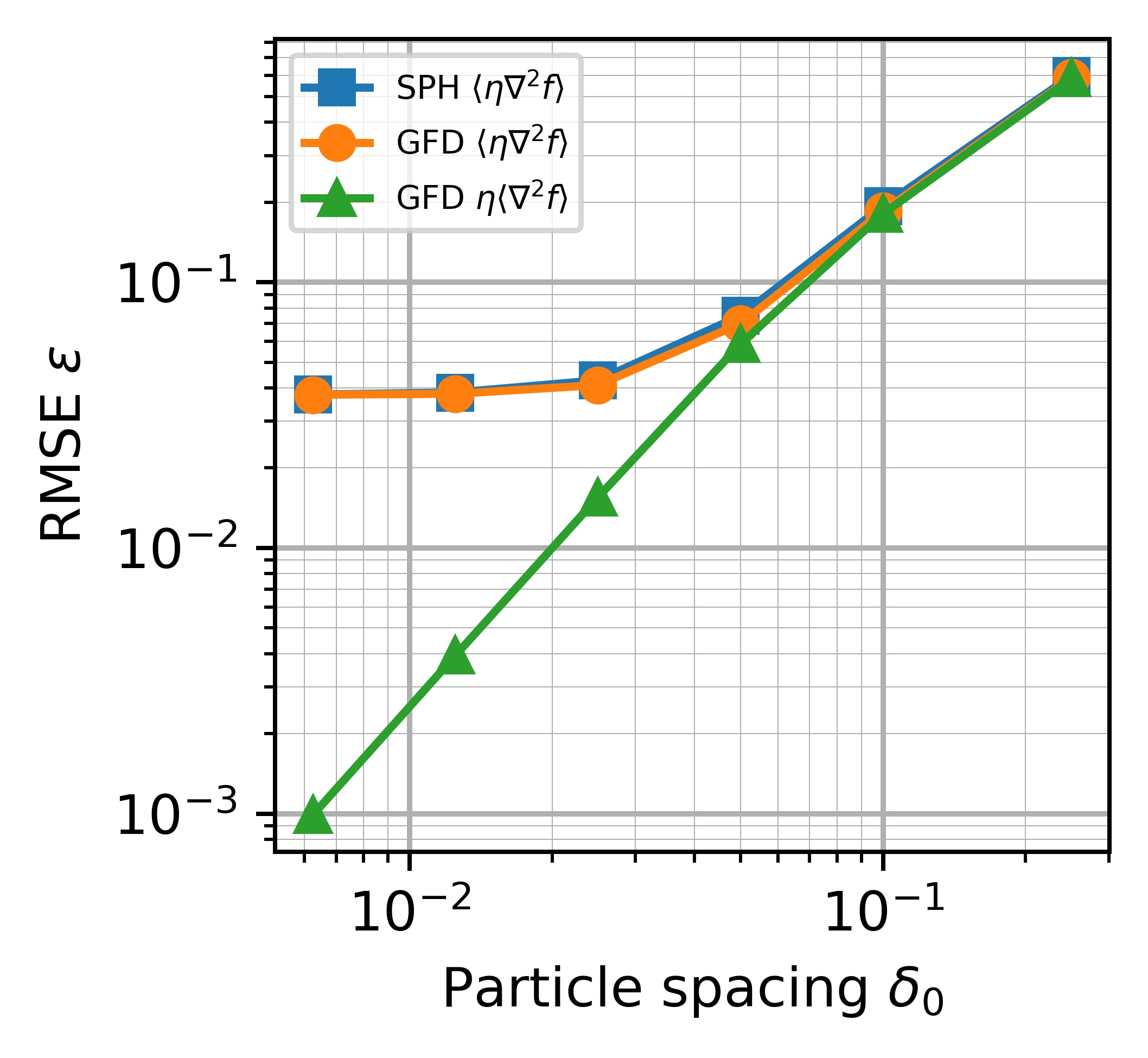
(a)

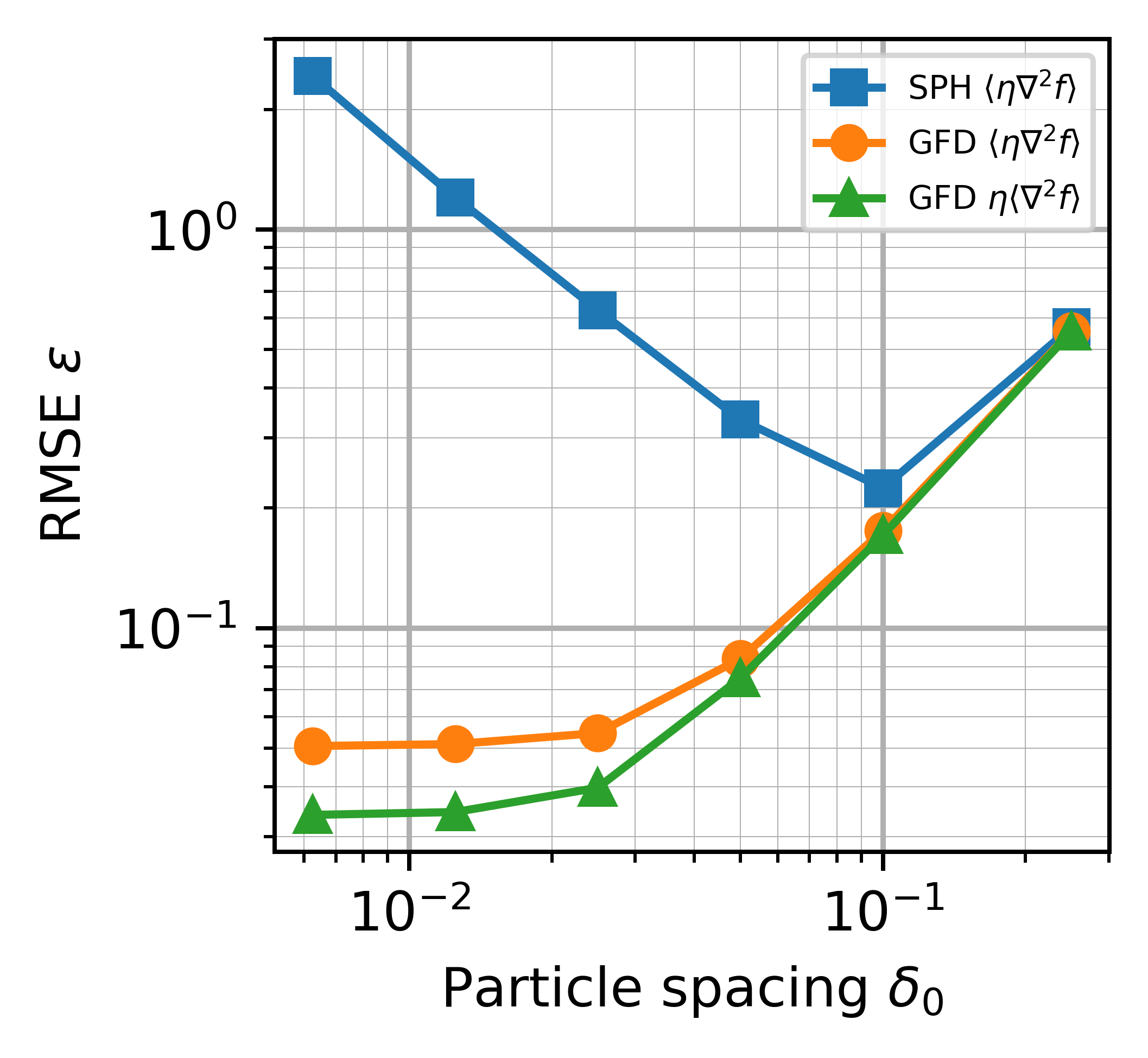
(b)

Figure 5: sph and gfd diffusion operators with varying viscosity rmse on a (a) regular and (b) irregular grid.

Of course, the rmse of $\eta\left<\nabla^{2}f\right>$ remains unchanged from the previous case. Both gfd and sph $\left<\eta\nabla^{2}f\right>$ show similar behavior on a regularly spaced grid. When comparing results on the irregular grid, it can be noticed that sph performs similarly to the previous case, showing no significant response to the introduction of a linearly-varying scalar field. Both gfd schemes have similar trends to the previous case, however, it is found that resolving $\eta\nabla^{2}f$ as $\eta\left<\nabla^{2}f\right>$ is more accurate than $\left<\eta\nabla^{2}f\right>$.

3.2 Multiphase Poiseuille flow

The next set of results considers the momentum diffusion operators applied to velocity fields in a multiphase flow environment. Specifically, the contributions towards momentum diffusion over the interface of the various schemes are quantified and compared against each other.

The numerical experiments are performed on velocity field solutions for multiphase Poiseuille flow between parallel plates. The velocity field is assigned according to the analytical results of [28]. Viscosity ratios $\mathcal{X}$ between 1:1 and 100:1 are considered in this study with the lower viscosity set to $\mu_{L}=1\text{Pa}\cdot\text{s}$ for all cases. All results in this section are considered on an irregular $20\times 40$ grid with $c=0.10$ over the domain $\left\{\left.x,y\in\mathbb{R}^{2}\right|0\leq x\leq 1,-1\leq y\leq 1\right\}$. As with the previous section, boundary particles are used to extend the computational domain and avoid kernel truncation. The same grid is used for all cases. A pressure gradient of $\frac{dp}{dx}=-1\text{N}/\text{m}^{3}$ is used to uniquely determine the velocity field. Figure 6 shows the velocity profile and particle distribution colored by dynamic viscosity for the $\mathcal{X}=5:1$ case. It should be emphasized that the particle viscosity is obtained from the color-weighted averaging scheme described in (7).

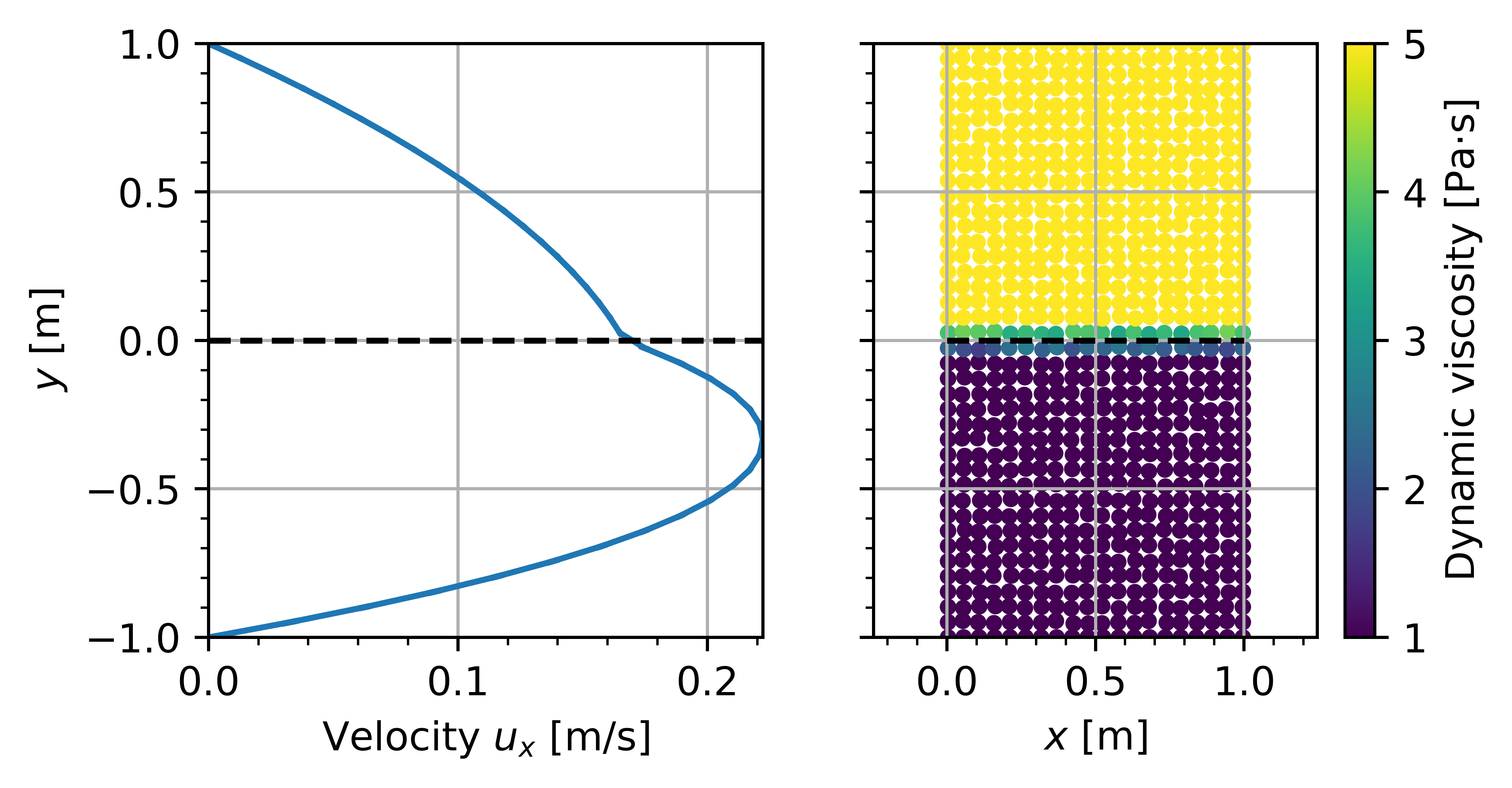
Figure 6: System configuration showing (a) the velocity profile and (b) the particle distribution colored by dynamic viscosity for the $\mathcal{X}=5:1$ case. The dashed line indicates the multiphase interface.

Figure 7 shows the diffusion operators’ responses averaged over the x-direction for different viscosity ratios. Figure 7(a) serves as a baseline with the gfd and sph operators applied to a single-phase case. Similar to the results of the previous section, it can be seen that the sph results are noisier than the gfd results due to grid irregularity. Figure 7(b) and Figure 7(c) shows results for $\mathcal{X}=5:1$ and $\mathcal{X}=100:1$, respectively. The behaviour of the gfd approximation $\mu\left<\nabla^{2}u_{x}\right>$ as well as the gfd and sph approximations $\left<\mu\nabla^{2}u_{x}\right>$ are provided. These results show that both the sph and gfd $\left<\mu\nabla^{2}u_{x}\right>$ diffusion operators have similar behavior in the multiphase region. It can be seen that $\left<\mu\nabla^{2}u_{x}\right>$ significantly under-predicts the value obtained from the post-multiplied diffusion operator $\mu\left<\nabla^{2}u_{x}\right>$.

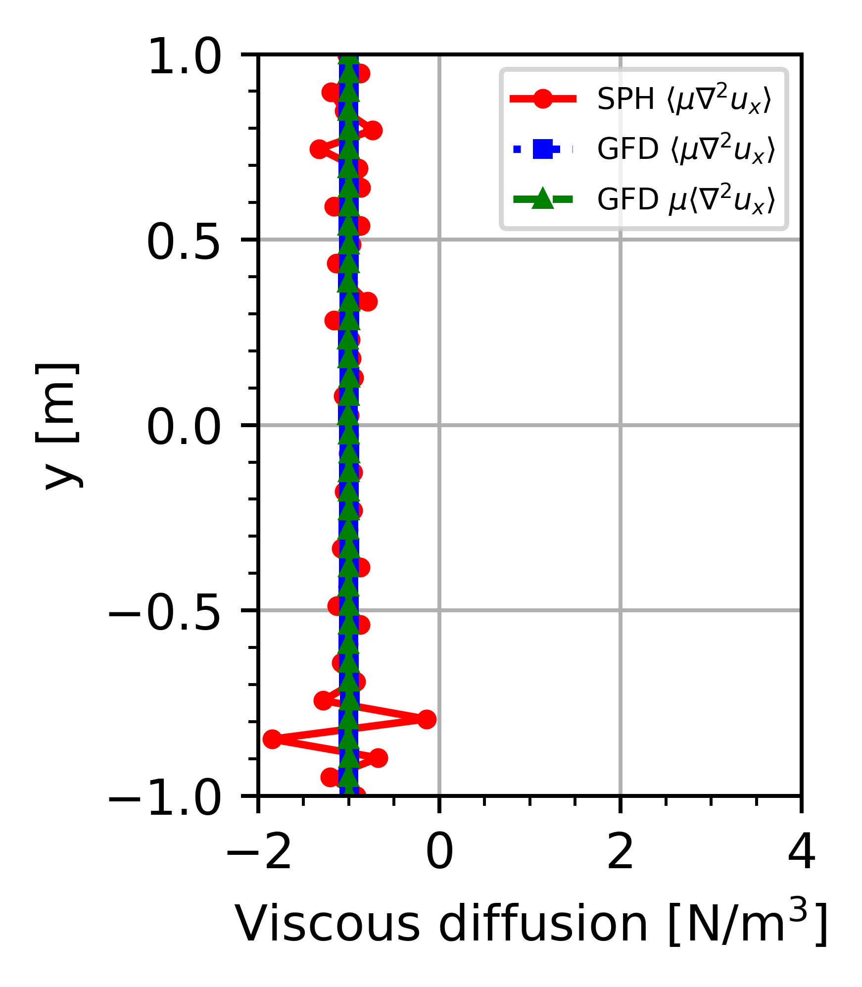
(a)

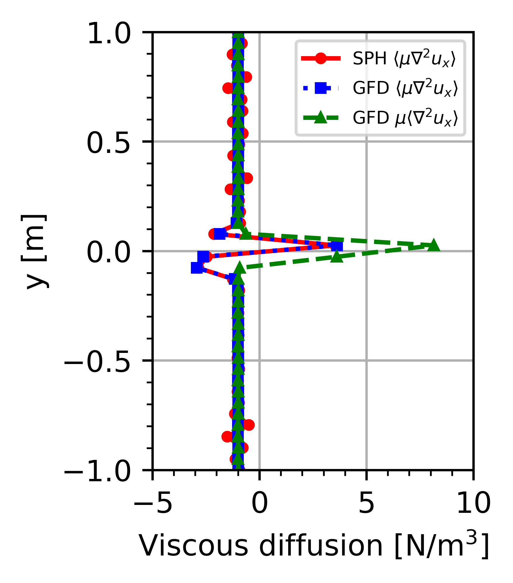
(b)

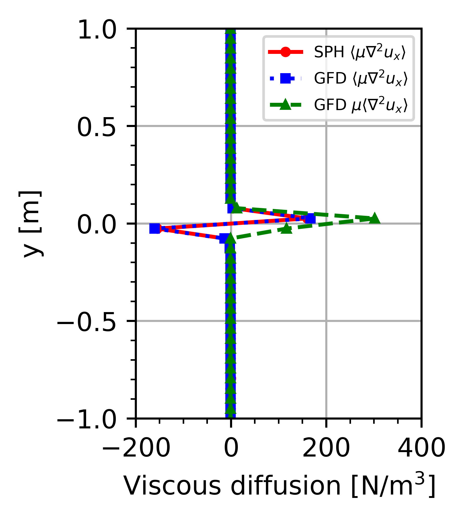
(c)

Figure 7: Averaged diffusion operator response for (a) $\mathcal{X}=1:1$, (a) $\mathcal{X}=5:1$ and (c) $\mathcal{X}=100:1$.

The shear divergence $\left<\nabla\cdot\mathbf{\tau}\right>$ is resolved with the gfd operators by resolving both $\mu\left<\nabla^{2}\mathbf{u}\right>$ and $\left<\nabla\mu\right>\cdot\left<2\mathbf{T}\right>$. To keep the accuracy and order of operators consistent in this comparison, the operator is only compared against the gfd $\left<\mu\nabla^{2}\mathbf{u}\right>$ operator. Furthermore, since the sph operator is shown to behave similarly in the interface region in a qualitative sense, the findings provide insight for the sph operators as well. It should be noted that $\left(\cdot\right)_{x}$ is used to indicate the x-component of a diffusion operator.

A comparison for $\mathcal{X}=1.3:1$, $\mathcal{X}=2:1$ and $\mathcal{X}=5:1$ is presented in Figure 8. It can be seen that $\left<\nabla\mu\right>\cdot\left<2\mathbf{T}\right>$ opposes the velocity Laplacian. As such, at lower viscosity ratios, this balances out the over-prediction of $\mu\left<\nabla^{2}\mathbf{u}\right>$ leading to $\left<\nabla\cdot\mathbf{\tau}\right>$ having a more similar response to $\left<\mu\nabla^{2}\mathbf{u}\right>$. However, as the viscosity ratio increases, $\left<\nabla\cdot\mathbf{\tau}\right>$ grows faster than $\left<\mu\nabla^{2}\mathbf{u}\right>$ leading to $\left<\nabla\cdot\mathbf{\tau}\right>$ predicting larger surface shear forces at the interface.

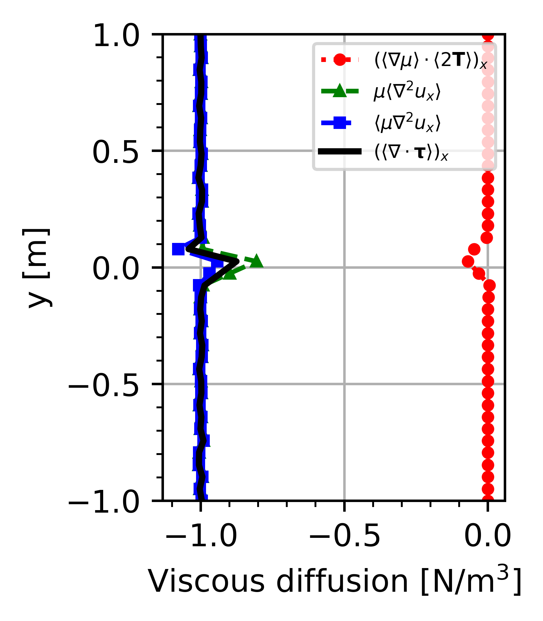
(a)

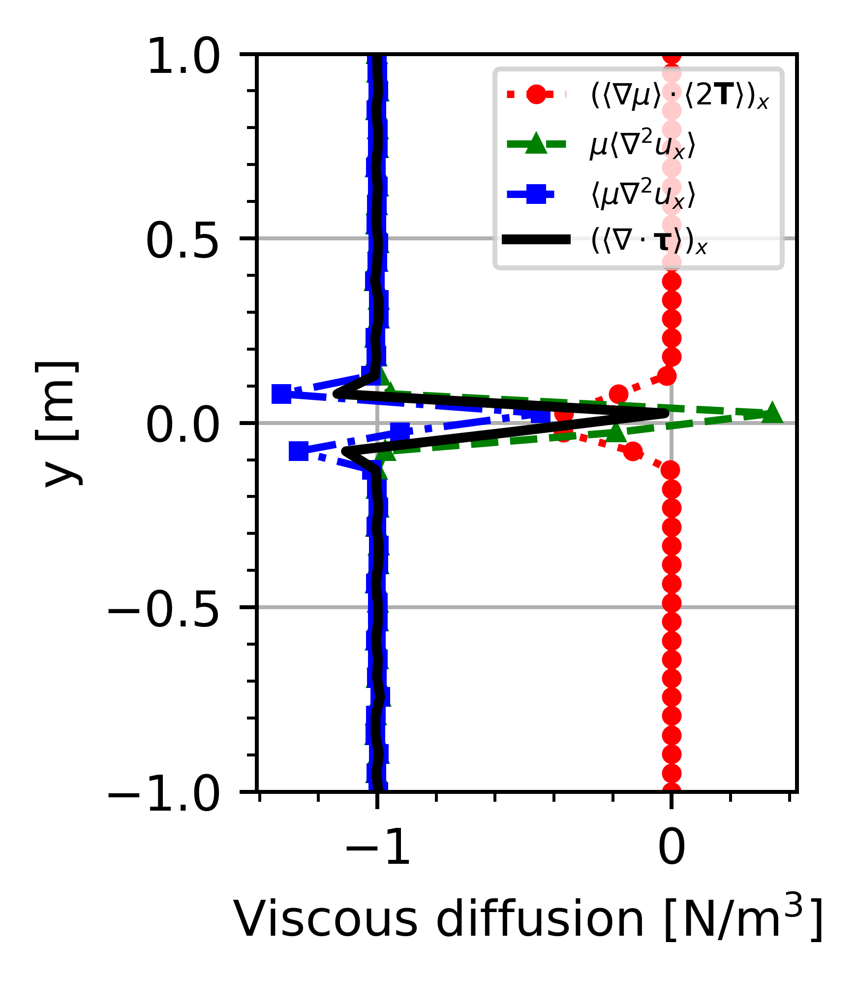
(b)

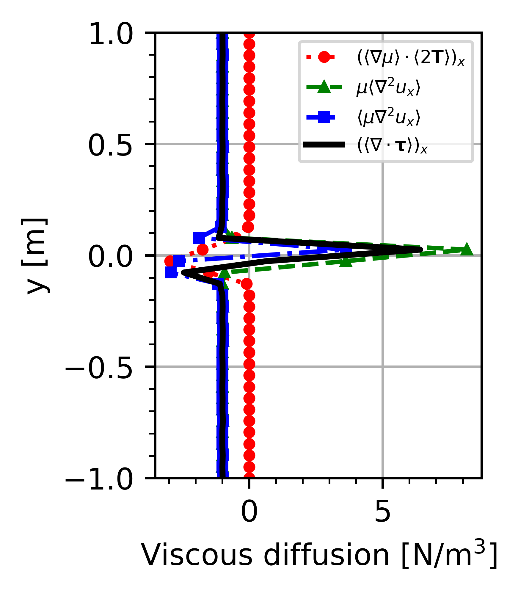
(c)

Figure 8: Comparison between gfd momentum diffusion operators for (a) $\mathcal{X}=1.3:1$, (a) $\mathcal{X}=2:1$ and (c) $\mathcal{X}=5:1$.

To quantify the difference between the operators, Figure 9 shows the rmse of the gfd and sph $\left<\mu\nabla^{2}\mathbf{u}\right>$ operators relative to the gfd $\left<\nabla\cdot\mathbf{\tau}\right>$ operator. Due to the high noise in the sph operator, the rmse is only considered over the domain $-3h\leq y\leq 3h$. As shown in the previous results, both sph and gfd obtain similar results. Here it is shown that at lower viscosity ratios, all operators predict similar behavior. However, as $\mathcal{X}$ increases, it can be seen that the viscosity discontinuity starts to dominate the surface shear prediction. The maximum disparity is found at that largest tested viscosity ratio of $\mathcal{X}=100:1$ where the rmse for the gfd and sph operators are 12.35 and 12.28, respectively.

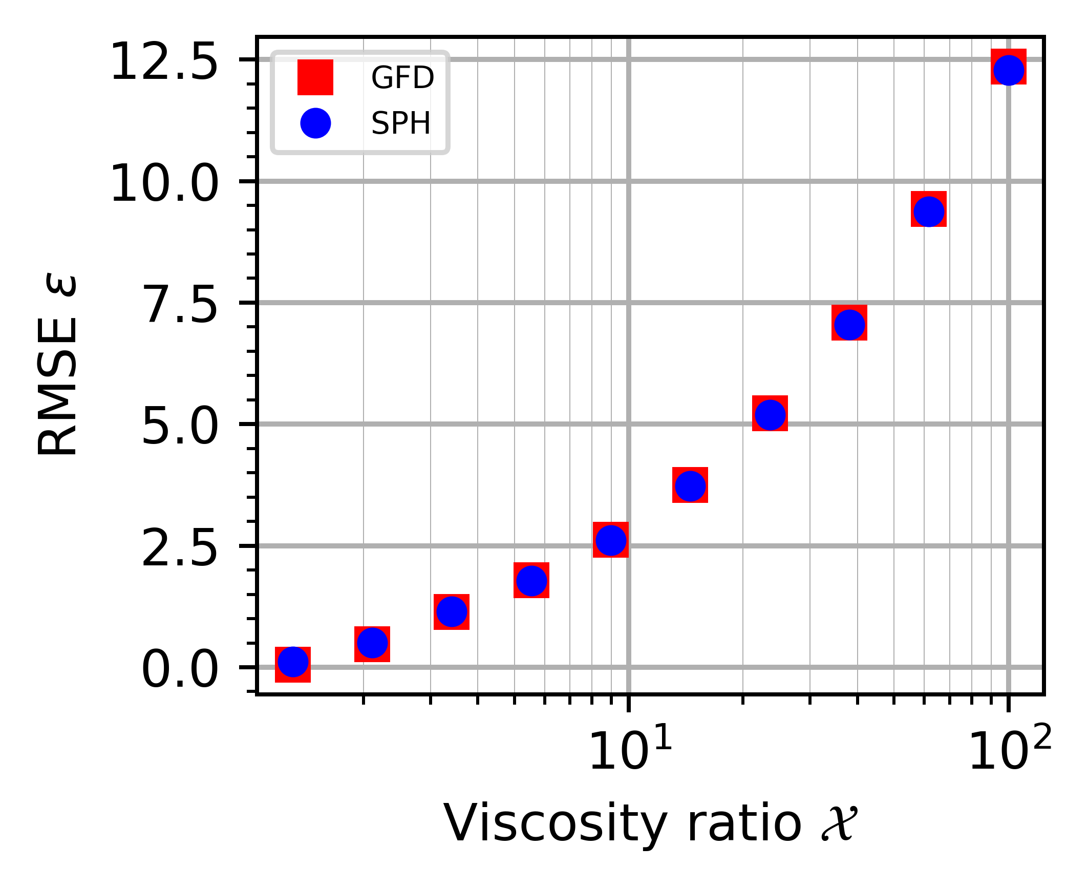
Figure 9: rmse of the gfd and sph $\left<\mu\nabla^{2}\mathbf{u}\right>$ diffusion operators over a viscosity ratio range of $\mathcal{X}=1.3:1$ and $\mathcal{X}=100:1$.

3.3 Rising bubble

The final section shows the effects that the choice of diffusion model has on the macroscopic system behavior. In this simulation, an initially spherical fluid is submerged in a heavier fluid. Buoyancy effects drive the evolution of the system and are balanced against the drag forces on the bubble surface. This system is particularly responsive to surface shear since it also partly drives the bubble’s deformation, which further influences the drag characteristics. Only the $\left<\mu\nabla^{2}\mathbf{u}\right>$ and $\left<\nabla\cdot\mathbf{\tau}\right>$ diffusion models resolved with gfd operators are compared in this section.

Full 3D simulations are performed with a schematic description of the initial condition shown in Figure 10. A bubble is initialized along the centerline of a cylindrical domain. The remaining volume of the cylinder is filled with a heavier fluid. Full-slip conditions are applied to the cylinder walls, while no-slip conditions are applied to the cylinder caps. A point-wise zero-pressure condition is enforced on the top cap at $(0,H-h_{0},0)$ to allow the pressure field to be uniquely resolved. The density and dynamic viscosity ratio between the fluids are set to $2:1$ and $100:1$, respectively. A lower density ratio is chosen to ensure that buoyancy doesn’t dominate viscous effects. The geometry is defined by $H=20D$, $W=2D$, $h_{0}=2D$ and $D=1$m. The bubble’s density and viscosity are given as $1\text{kg}/\text{m}^{3}$ and $2/875\text{Pa}\cdot s$. The system configuration is determined by the Reynolds number $Re=\rho_{2}DU_{g}/\mu_{2}$ and Weber number $We=\rho_{2}DU_{g}^{2}/\sigma$ with $U_{g}=\sqrt{gD}$ the characteristic velocity. The gravitational acceleration and surface tension coefficient are chosen such that $Re=8.75$ and $We=116$. This results in $g=1\text{m}/\text{s}^{2}$ and $\sigma=1/58$N/m. It should be noted that gravity is incorporated as a buoyancy force and as such, $\mathbf{g}_{i}=(1-\rho_{i}/\rho_{2})\mathbf{g}_{0}$. The initial particle spacing is set to $\delta_{0}=31.25$mm leading to a simulation with 4M particles.

Figure 10: Schematic description of the rising bubble case.

Two simulations are performed in this section, with one simulation making use of the $\left<\mu\nabla^{2}\mathbf{u}\right>$ diffusion model and the other making use of the $\left<\nabla\cdot\mathbf{\tau}\right>$ diffusion model. Besides the diffusion operator, the simulations are identical.

Figure 11 shows the pressure and velocity fields of the bubbles at $t=7$s. Immediately, it can be seen that the bubble velocity is significantly lower for the $\left<\nabla\cdot\mathbf{\tau}\right>$ operator. Conversely, the pressure fields are similar in both magnitude and shape with $\Delta p=0.759$Pa and $\Delta p=0.782$Pa for the $\left<\mu\nabla^{2}\mathbf{u}\right>$ and $\left<\nabla\cdot\mathbf{\tau}\right>$ cases, respectively. This is a result of buoyancy being the primary driver behind the pressure response. This indicates that the difference in bulk bubble kinematics can primarily be attributed to the viscous diffusion rate.

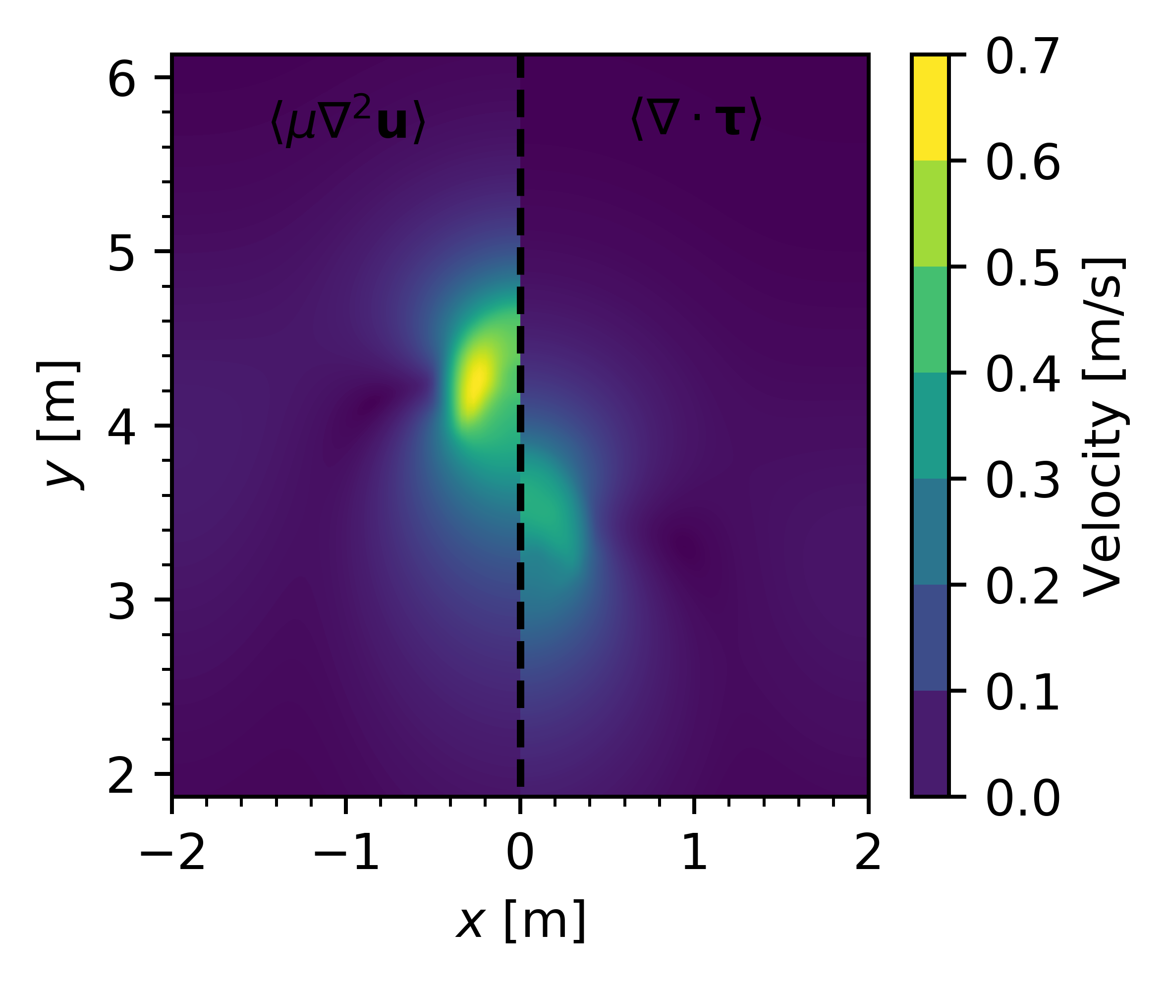
(a)

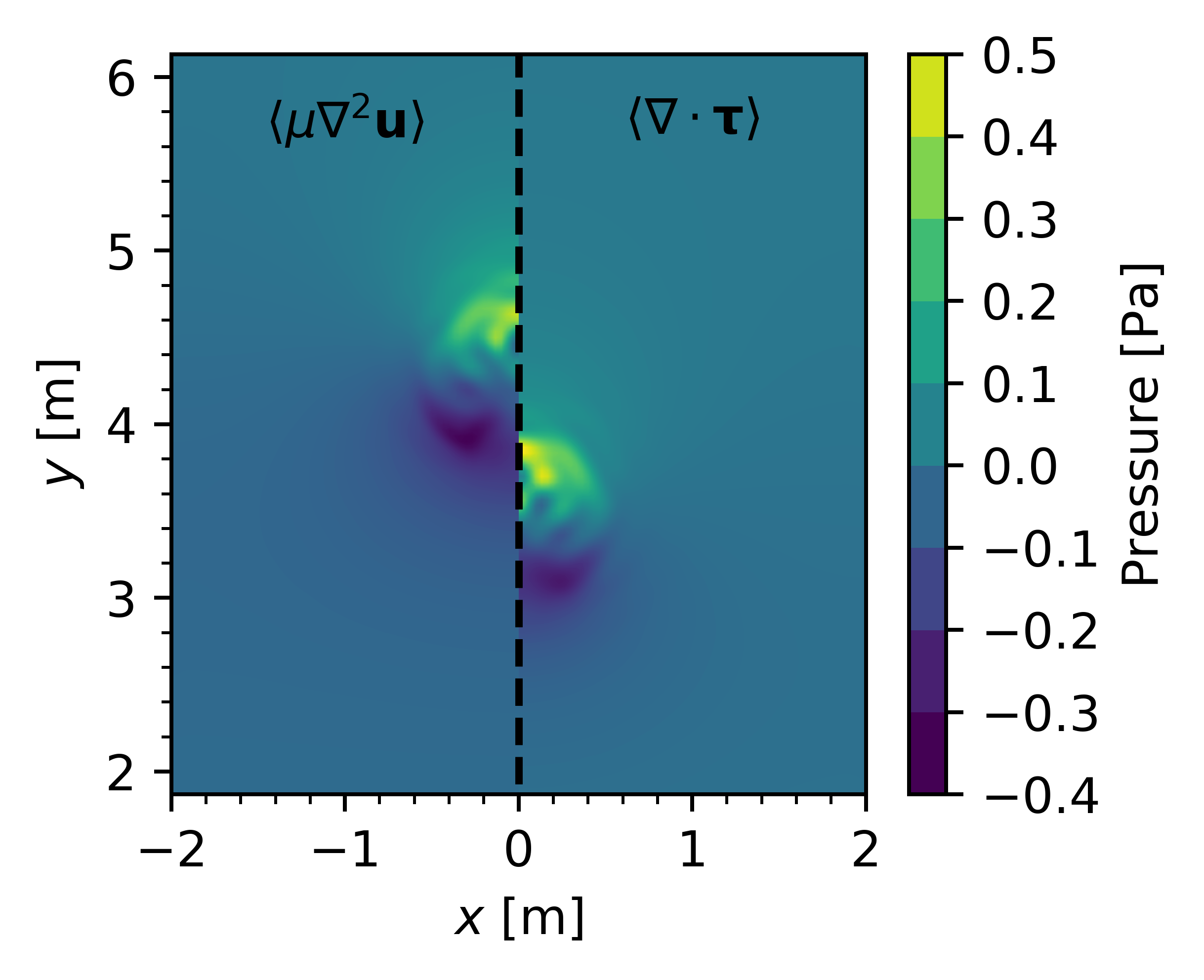
(b)

Figure 11: Comparison between (a) velocity and (b) pressure fields near the bubble at $t=7$s obtained with the $\left<\mu\nabla^{2}\mathbf{u}\right>$ and $\left<\nabla\cdot\mathbf{\tau}\right>$ momentum diffusion models.

The next set of results compares the steady-state bubble shape as seen in Figure 12. The shape is obtained by applying a Shepard filter to the color field $C^{0}$ and resolving the contour at $C^{0}=0.5$. It can be noted that the bubble shape is qualitatively similar, although subtle differences can be seen. Specifically, the $\left<\mu\nabla^{2}\mathbf{u}\right>$ case predicts a slightly wider and flatter bubble. Furthermore, the bottom surface has a more exaggerated profile. These differences in bubble shape follow a similar trend observed in [29] when increasing the density ratio and thus increasing the ascent rate while fixing $Re=8.75$, $We=116$ and $\mathcal{X}=100:1$. The effects are not as pronounced as [29], likely due to the similar densities between phases.

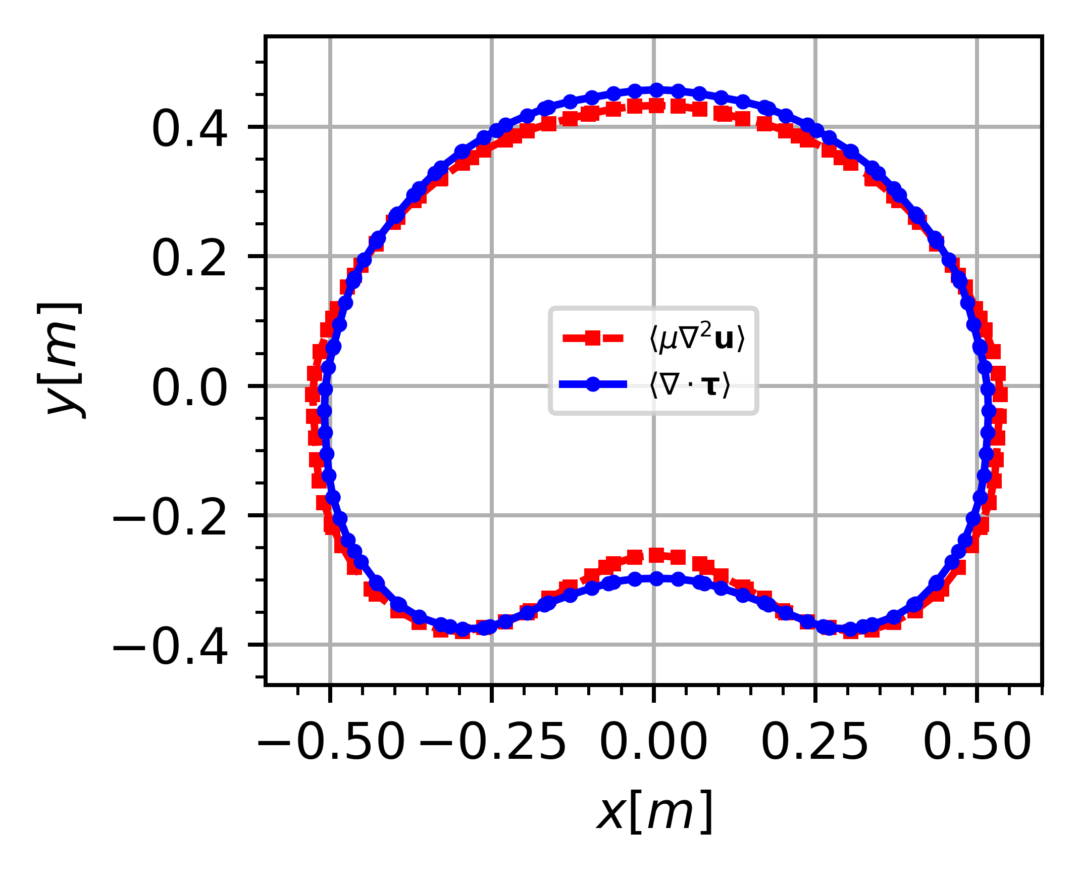
Figure 12: Steady state bubble shapes for the $\left<\mu\nabla^{2}\mathbf{u}\right>$ and $\left<\nabla\cdot\mathbf{\tau}\right>$ diffusion models.

Figure 13 shows the average vertical velocity of the bubble. As shown in the previous results, the $\left<\mu\nabla^{2}\mathbf{u}\right>$ diffusion operator under-predicts the surface shear. This leads to the $\left<\mu\nabla^{2}\mathbf{u}\right>$ case to predict a higher terminal velocity with a difference of 57.2% relative to the $\left<\nabla\cdot\mathbf{\tau}\right>$ case. When compared to the terminal velocity obtained in [29] using a fvm, the $\left<\nabla\cdot\mathbf{\tau}\right>$ diffusion operator predicts similar bubble kinematics. This is expected as [29] appropriately resolved the fluid momentum diffusion as $\nabla\cdot\mathbf{\tau}$.

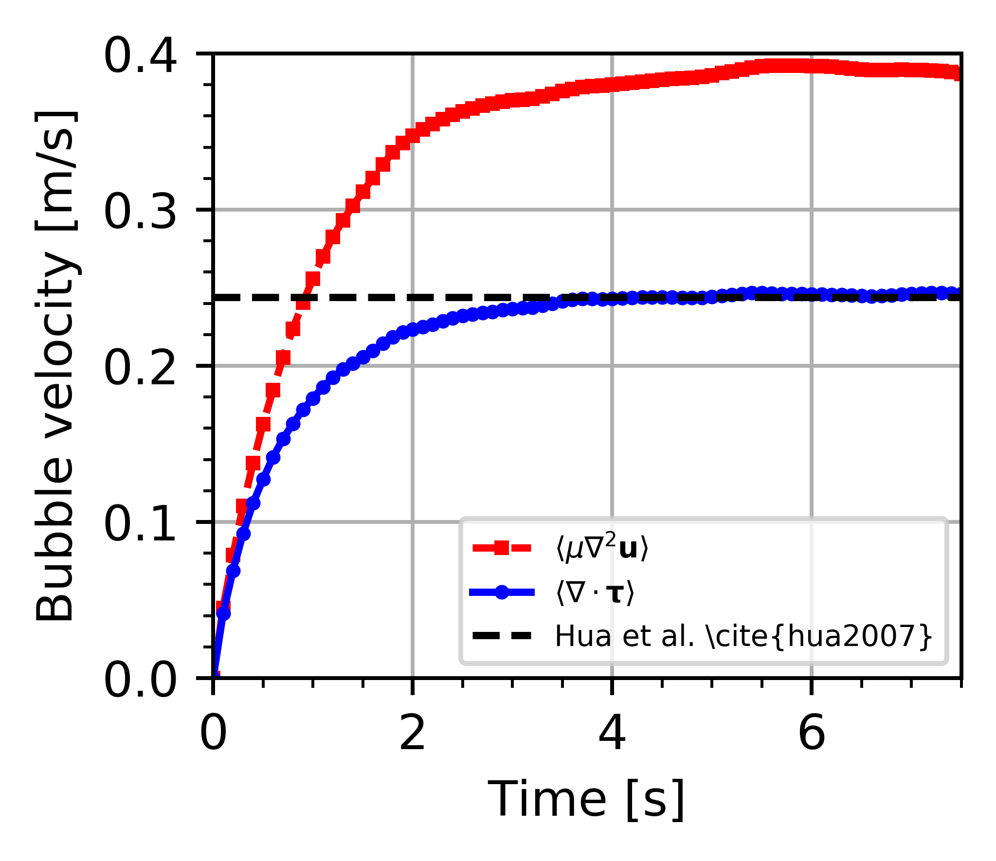
Figure 13: Time evolution of the bubble’s bulk vertical velocity for both the $\left<\mu\nabla^{2}\mathbf{u}\right>$ and $\left<\nabla\cdot\mathbf{\tau}\right>$ momentum diffusion models.

4 Conclusion

This work presents a comparison between mlm momentum diffusion models for multiphase flow. The common momentum diffusion operators for sph and gfd are compared to a gfd operator that includes the effects of viscosity sensitivity at multiphase interfaces. A computationally efficient model for the viscosity gradient based on the color gradient is proposed as part of this work.

It was shown that although the gfd operator was less susceptible to irregular spacing due to it being first-order accurate, both the sph and gfd $\left<\mu\nabla^{2}\mathbf{u}\right>$ momentum diffusion operators behave similarly at multiphase interfaces. Specifically, both under-estimate surface shear with the error growing as the viscosity ratio increases.

The significance of this effect is demonstrated by simulating the evolution of a bubble submerged in a heavy fluid. The reduced surface shear resulted in a significant over-prediction of the bubble’s terminal velocity despite resolving similar pressure conditions. Specifically, the ascent velocity is over-predicted by 57.2%when modelling momentum diffusion as $\left<\mu\nabla^{2}\mathbf{u}\right>$ compared to $\left<\nabla\cdot\mathbf{\tau}\right>$ at a density ratio of $2:1$ and a viscosity ratio of $100:1$.

This indicates that the viscosity gradient cannot be ignored when constructing the momentum diffusion operator for multiphase flow, especially when viscous effects are relatively strong. As such, this work recommends that multiphase gfd solvers make use of the proposed $\left<\nabla\cdot\mathbf{\tau}\right>$ diffusion model. Furthermore, due to the similarity between the sph and gfd momentum diffusion operators highlighted in this work, the proposed diffusion operator should be explored in a sph context as well.

5 References

References

- [1] J. Brackbill, D. Kothe, C. Zemach, A continuum method for modeling surface tension, Journal of Computational Physics 100 (2) (1992) 335–354.
- [2] X. Hu, N. Adams, A multi-phase sph method for macroscopic and mesoscopic flows, Journal of Computational Physics 213 (2) (2006) 844–861.
- [3] S. Adami, X. Y. Hu, N. A. Adams, A new surface-tension formulation for multi-phase sph using a reproducing divergence approximation, Journal of Computational Physics 229 (13) (2010) 5011–5021.
- [4] X. Y. Hu, N. A. Adams, An incompressible multi-phase sph method, Journal of Computational Physics 227 (1) (2007) 264–278.
- [5] X. Y. Hu, N. A. Adams, A constant-density approach for incompressible multi-phase sph, Journal of Computational Physics 228 (6) (2009) 2082–2091.
- [6] A. Zainali, N. Tofighi, M. S. Shadloo, M. Yildiz, Numerical investigation of newtonian and non-newtonian multiphase flows using isph method, Computer Methods in Applied Mechanics and Engineering 254 (2013) 99–113.
- [7] A. Shakibaeinia, Y.-C. Jin, Mps mesh-free particle method for multiphase flows, Computer Methods in Applied Mechanics and Engineering 229-232 (2012) 13–26.
- [8] A. Khayyer, H. Gotoh, Enhancement of performance and stability of mps mesh-free particle method for multiphase flows characterized by high density ratios, Journal of Computational Physics 242 (2013) 211–233.
- [9] T. Douillet-Grellier, S. Leclaire, D. Vidal, F. Bertrand, F. De Vuyst, Comparison of multiphase sph and lbm approaches for the simulation of intermittent flows, Computational Particle Mechanics 6 (4) (2019) 695–720.
- [10] S. Geara, S. Martin, S. Adami, W. Petry, J. Allenou, B. Stepnik, O. Bonnefoy, A new sph density formulation for 3d free-surface flows, Computers & Fluids 232 (2022) 105193.
- [11] L. Yang, M. Rakhsha, W. Hu, D. Negrut, A consistent multiphase flow model with a generalized particle shifting scheme resolved via incompressible sph, Journal of Computational Physics 458.
- [12] J. P. Morris, P. J. Fox, Y. Zhu, Modeling low reynolds number incompressible flows using sph, Journal of Computational Physics 136 (1) (1997) 214–226.
- [13] J. Monaghan, R. Gingold, Shock simulation by the particle method sph, Journal of Computational Physics 52 (2) (1983) 374–389.
- [14] F. R. Ming, P. N. Sun, A. M. Zhang, Numerical investigation of rising bubbles bursting at a free surface through a multiphase sph model, Meccanica 52 (11-12) (2017) 2665–2684.
- [15] M.-K. Li, A.-M. Zhang, F.-R. Ming, P.-N. Sun, Y.-X. Peng, An axisymmetric multiphase sph model for the simulation of rising bubble, Computer Methods in Applied Mechanics and Engineering 366 (2020) 113039.
- [16] H. Cheng, Y. Liu, F. Ming, P. Sun, Investigation on the bouncing and coalescence behaviors of bubble pairs based on an improved apr-sph method, Ocean Engineering 255.
- [17] F. He, H. Zhang, C. Huang, M. Liu, A stable sph model with large cfl numbers for multi-phase flows with large density ratios, Journal of Computational Physics 453.
- [18] N. Lanson, J. P. Vila, Renormalized meshfree schemes i: Consistency, stability, and hybrid methods for conservation laws, SIAM Journal on Numerical Analysis 46 (4) (2008) 1912–1934.
- [19] N. Lanson, J. P. Vila, Renormalized meshfree schemes ii: Convergence for scalar conservation laws, SIAM Journal on Numerical Analysis 46 (4) (2008) 1935–1964.
- [20] J. Basic, N. Degiuli, D. Ban, A class of renormalised meshless laplacians for boundary value problems, Journal of Computational Physics 354 (2018) 269–287.
- [21] J. C. Joubert, D. N. Wilke, N. Govender, P. Pizette, J. Basic, N. E. Abriak, Boundary condition enforcement for renormalised weakly compressible meshless lagrangian methods, Engineering Analysis with Boundary Elements 130 (2021) 332–351.
- [22] J. Basic, B. Blagojevic, M. Andrun, N. Degiuli, A lagrangian finite difference method for sloshing: Simulations and comparison with experiments, in: Proceedings of the Twenty-ninth International Ocean and Polar Engineering Conference, 2019, pp. 3412–3418.
- [23] J. C. Joubert, N. Govender, D. N. Wilke, P. Pizette, A meshless lagrangian particle-based porosity formulation for under-resolved generalised finite difference-dem coupling in fluidised beds, Powder Technology 398.
- [24] D. Shepard, A two-dimensional interpolation function for irregularly-spaced data, in: Proceedings of the 1968 23rd ACM National Conference, ACM ’68, Association for Computing Machinery, New York, NY, USA, 1968, p. 517–524.
- [25] Q. Yang, F. Xu, Y. Yang, L. Wang, A multi-phase sph model based on riemann solvers for simulation of jet breakup, Engineering Analysis with Boundary Elements 111 (2020) 134–147.
- [26] R. Xu, P. Stansby, D. Laurence, Accuracy and stability in incompressible sph (isph) based on the projection method and a new approach, Journal of Computational Physics 228 (18) (2009) 6703–6725.
- [27] R. Franke, A critical comparison of some methods for interpolation of scattered data, Tech. Rep. NPS-53-79-003, Naval Postgraduate School Tech. Rep. (1979).
- [28] R. Bird, W. Stewart, E. Lightfoot, Transport Phenomena, Wiley, 2002.
- [29] J. Hua, J. Lou, Numerical simulation of bubble rising in viscous liquid, Journal of Computational Physics 222 (2) (2007) 769–795.