Rate-Adaptive Protograph MacKay-Neal Codes

Abstract

A class of rate-adaptive protograph MacKay-Neal (MN) codes is introduced and analyzed. The code construction employs an outer distribution matcher (DM) to adapt the rate of the scheme. The DM is coupled with an inner protograph-based low-density parity-check (LDPC) code, whose base matrix is optimized via density evolution analysis to approach the Shannon limit of the binary-input additive white Gaussian noise (biAWGN) channel over a given range of code rates. The density evolution analysis is complemented by finite-length simulations, and by a study of the error floor performance.

I Introduction

MacKay-Neal (MN) codes were introduced in [1, Sec. VI] as a class of error correcting codes based on sparse matrices for nonuniform sources. They can be seen as multi-edge-type low-density parity-check (LDPC) codes [2, 3] defined by an extended bipartite graph with a set of variable nodes associated with the source bits, and the remaining VNs associated with the codeword bits. LDPC code constructions closely related to MN codes were proposed in [4, 5] for joint source and channel coding. While originally introduced to deal with nonuniform sources, it was pointed out in [1] that MN can be employed also with uniform sources, by introducing a nonlinear block code that turns the uniform source output sequence into a sequence with a prescribed distribution. In [1] it was also recognized that this option may be appealing from a rate flexibility viewpoint, since the rate of the scheme may be modified (e.g., adapted to varying channel conditions) by changing the statistics of the sequences produced by the nonlinear block encoder, hence without modifying the underlying LDPC code. This approach is interesting from two viewpoints. First, the possibility of adapting the rate without changing the underlying LDPC encoder/decoder is important to limit the implementation complexity (modern communication standards that seek rate flexibility often specify a large number of LDPC code parity-check matrices to serve different rates, see e.g. [6]). Second, a rate-adaptive scheme based on MN codes allows to keep the block length constant, allowing the introduction of periodic synchronization markers, with benefits in terms of frame synchronization performance. Despite these appealing properties, MN codes as a means to achieve rate flexibility received little attention. A notable exception is the probabilistic amplitude shaping (PAS) scheme introduced in [7], where a construction reminiscent of MN codes was proposed. In PAS, the sequence output by a uniform (binary) source is also processed by the nonlinear block encoder, referred to as distribution matcher (DM) [7], generating a sequence of amplitude symbols with a given empirical distribution. The binary labels associated with the amplitude symbols are encoded through a nonsystematic LDPC code encoder, producing a parity bit vector. The amplitude symbols together with the parity bits are then mapped onto pulse amplitude modulation (PAM) symbols. While the main result achieved by PAS is to provide sizable shaping gains, it was quickly recognized that, as a byproduct, PAS is naturally rate-adapting thanks to the possibility of tuning the DM rate [7], as originally hypothesized in [1]. This aspect makes PAS attractive for optical long haul transmission systems [8].

In this paper, we analyze and design a class of rate-adaptive MN codes for the binary-input additive white Gaussian noise (biAWGN) channel. The class is based on protograph LDPC codes [9] coupled with a constant composition distribution matcher (CCDM) [7, 10]. Noting that the concatenation of the CCDM with the inner linear block code results in a nonlinear code, we introduce an equivalent decoding problem. The equivalent problem resorts to the study of the performance of the protograph LDPC code over the communication channel, where side information is provided to the decoder by observing the LDPC encoder input through a binary-input, binary-output channel. By means of protograph extrinsic information transfer (PEXIT) analysis [11, 12], we design rate-adaptive MN codes that are capable of operating close to the biAWGN channel capacity over a wide range of code rates. A quantized density evolution (DE) analysis [13] is used to confirm the accuracy of the thresholds computed via PEXIT analysis. Finite-length performance results are finally included, and complemented by an error floor analysis that (for the designed codes) yields precise estimates of the code performance at large signal-to-noise ratios.

Figure 1: System model, where a MN code is used to communicate over the biAWGN channel (communication channel).

II Preliminaries

In the following, we denote random variables by uppercase letters and their realisations by lowercase letters. We denote the probability mass function (p.m.f.) of a discrete r.v. $X$ as $P_{X}(x)=\mathsf{P}\!\left[X=x\right]$, and the probability density function (p.d.f.) of discrete r.v. $X$ as $p_{X}(x)$. In either case, the subscript will be dropped whenever the context allows it, i.e., $P(x)=P_{X}(x)$ and $p(x)=p_{X}(x)$. We use $\mathsf{H}_{\scaleto{\mathsf{b}}{4pt}}(\omega)$ to denote the binary entropy function, i.e., $\mathsf{H}_{\scaleto{\mathsf{b}}{4pt}}(\omega)=-\omega\log_{2}\omega-(1-\omega)\log_{2}(1-\omega)$ for $0<\omega<1$ and $\mathsf{H}_{\scaleto{\mathsf{b}}{4pt}}(0)=\mathsf{H}_{\scaleto{\mathsf{b}}{4pt}}(1)=0$. We refer to vectors as row vectors denoted by bold letters, e.g., $\bm{x}$, whereas matrices are denoted by uppercase bold letters, e.g., $\bm{X}$. We denote by $\mathbbmss{F}_{\!\scaleto{\mathsf{2}}{3.5pt}}$ the order-$2$ finite field. We use $w_{\scaleto{\mathsf{H}}{3.5pt}}(\bm{x})$ and $d_{\scaleto{\mathsf{H}}{3.5pt}}(\bm{x},\bm{y})$ to be respectively the Hamming weight of a vector $\bm{x}$ and the Hamming distance between two vectors $\bm{x}$ and $\bm{y}$.

We consider transmission over the biAWGN channel defined by $Y=X+N$ where $Y$ is the channel output, $X\in\{-1,+1\}$ is the channel input, and where $N\sim\mathcal{N}(0,\sigma^{2})$ is the additive white Gaussian noise term. The channel SNR is defined as $E_{s}/N_{0}=1/(2\sigma^{2})$ where $E_{s}$ is the energy per symbol and $N_{0}$ is the single-sided noise power spectral density.

II-A Protograph LDPC codes

A protograph $\mathcal{P}$ is a small bipartite graph consisting of a set of $n_{0}$ VNs, a set of $m_{0}$ check nodes, and $e$ edges. VNs in the protograph are numbered from $1$ to $n_{0}$. Similarly, protograph CNs are numbered from $1$ to $m_{0}$. Each VN/CN/edge in a protograph defines a VN/CN/edge type. The bipartite graph $\mathcal{G}$ of an LDPC code can be derived by lifting the protograph. In particular, the protograph is copied ${\ell}$ times (where ${\ell}$ is referred to as the lifting factor), and the edges of the protograph copies are permuted under the following constraint: if an edge connects a type-$j$ VN to a type-$i$ CN in $\mathcal{P}$, after permutation the edge should connect one of the ${\ell}$ type-$j$ VN copies with one of the ${\ell}$ type-$i$ CN copies in $\mathcal{G}$. We denote by $\{\mathsf{v}_{1},\mathsf{v}_{2},\ldots,\mathsf{v}_{n}\}$ the set of $n={\ell}n_{0}$ VNs in $\mathcal{G}$, and by $\{\mathsf{c}_{1},\mathsf{c}_{2},\ldots,\mathsf{c}_{m}\}$ the set of $m={\ell}m_{0}$ CNs. The lifted graph $\mathcal{G}$ defines the $m\times n$ parity-check matrix $\bm{H}$. The base matrix of a protograph is an $m_{0}\times n_{0}$ matrix $\bm{B}=[b_{i,j}]$ where $b_{i,j}$ is the number of edges that connect VN $j$ to CN $i$ in $\mathcal{P}$. We will make use of LDPC codes with punctured (or state) VNs. A punctured VN is associated with a codeword bit that is not transmitted through the communication channel. We will assume that all the VNs of a given type are either punctured, or they are not.

III Protograph MacKay-Neal Codes

A MN code can be constructed by concatenating an outer nonlinear code $\mathcal{C}_{\scaleto{\mathsf{O}}{3.5pt}}$ with an inner code $\mathcal{C}_{\scaleto{\mathsf{I}}{3.5pt}}$ [1]. More specifically, we consider the setting depicted in Figure 1. Here, an independent and identically-distributed (i.i.d.) uniform source generates a message $\mu\in\{1,2,\ldots,M\}$. The message is input to the encoder of an length-$h$ outer code $\mathcal{C}_{\scaleto{\mathsf{O}}{3.5pt}}$ whose task is to generate an output sequence with a prescribed empirical distribution. Following [7], we refer to such a device as the DM. We restrict out attention to DMs based on constant composition (CC) codes which admit low-complexity implementation via arithmetic coding [1, 10] . Let $\omega\in(0,1)$ denote the fractional Hamming weight of the $h$-bits vector $\bm{v}$, i.e., $\omega=w_{\scaleto{\mathsf{H}}{3.5pt}}(\bm{v})/h$. We have that $M=|\mathcal{C}_{\scaleto{\mathsf{O}}{3.5pt}}|={h\choose\omega h}$. Hence, the rate of the outer code is $R_{\scaleto{\mathsf{O}}{3.5pt}}=h^{-1}\log_{2}M=h^{-1}\log_{2}{h\choose\omega h}$, which converges to $\mathsf{H}_{\scaleto{\mathsf{b}}{4pt}}(\omega)$ for large $h$. The output of the DM is then input to the encoder of an inner $(n,h)$ binary linear block code $\mathcal{C}_{\scaleto{\mathsf{I}}{3.5pt}}$. The inner code $\mathcal{C}_{\scaleto{\mathsf{I}}{3.5pt}}$ is defined by

$$\mathcal{C}_{\scaleto{\mathsf{I}}{3.5pt}}=\left\{\bm{c}\big{|}\bm{c}\bm{H}_{2}^{\scaleto{\mathsf{T}}{3.5pt}}=\bm{v}\bm{H}_{1}^{\scaleto{\mathsf{T}}{3.5pt}},\bm{v}\in\mathbbmss{F}_{\!\scaleto{\mathsf{2}}{3.5pt}}^{h}\right\}$$ (1)

where $\bm{H}_{1}$ is an $n\times h$ sparse binary matrix, and $\bm{H}_{2}$ is an $n\times n$ sparse binary matrix. Note that, strictly speaking, $\mathcal{C}_{\scaleto{\mathsf{I}}{3.5pt}}$ may not be an LDPC code, i.e., the code may not possess a sparse parity-check matrix. Nevertheless, $\mathcal{C}_{\scaleto{\mathsf{I}}{3.5pt}}$ can be seen as the code obtained by puncturing an $(n+h,h)$ LDPC code with $n\times(h+n)$ parity-check matrix

$$\bm{H}=\left[\,\bm{H}_{1}\,|\,\bm{H}_{2}\,\right]$$ (2)

where puncturing is applied to the first $h$ coordinates. We refer to the $(n+h,h)$ LDPC code with parity-check matrix in the form (2) as the (inner) mother code $\mathcal{C}_{\scaleto{\mathsf{IM}}{3.5pt}}$. The inner code rate is $R_{\scaleto{\mathsf{I}}{3.5pt}}=h/n$, whereas the mother code rate is $R_{\scaleto{\mathsf{IM}}{3.5pt}}=h/(n+h)=R_{\scaleto{\mathsf{I}}{3.5pt}}/(1+R_{\scaleto{\mathsf{I}}{3.5pt}})$. We assume $\bm{H}_{2}$ to possess rank $n$, implying that $\bm{H}_{2}$ is invertible. We denote by $\bm{G}=\bm{H}_{1}\bm{H}_{2}^{-{\scaleto{\mathsf{T}}{3.5pt}}}$ the generator matrix of the inner code $\mathcal{C}_{\scaleto{\mathsf{I}}{3.5pt}}$. Note that if the inverse of $\bm{H}_{2}$ is dense, then the generator matrix $\bm{G}$ is dense. It follows that the concatenation of the outer CC code with the inner linear block code yields a marginal distribution of the codeword bits that is close to uniform, as required by the capacity-achieving input distribution of the biAWGN channel [7]. The overall code obtained by the concatenation of the outer CC code and the inner binary linear block code is denoted by $\mathcal{C}$, and its rate is $R=R_{\scaleto{\mathsf{O}}{3.5pt}}R_{\scaleto{\mathsf{I}}{3.5pt}}\approx\mathsf{H}_{\scaleto{\mathsf{b}}{4pt}}(\omega)R_{\scaleto{\mathsf{I}}{3.5pt}}$. We remark that all rates $0<R<R_{\scaleto{\mathsf{I}}{3.5pt}}$ can be achieved simply by fixing the DM parameter, hence its rate, without performing any modification (e.g., puncturing/shortening) to the inner code.

We consider MN codes based on a protograph mother LDPC code $\mathcal{C}_{\scaleto{\mathsf{IM}}{3.5pt}}$. In particular, the mother code parity-check matrix (2) is obtained by lifting a protograph whose $n_{0}\times(h_{0}+n_{0})$ base matrix takes the form $\bm{B}=\left[\,\bm{B}_{1}\,|\,\bm{B}_{2}\,\right]$ where $\bm{B}_{1}$ has dimensions $n_{0}\times h_{0}$ and $\bm{B}_{2}$ has dimensions $n_{0}\times n_{0}$, where $n_{0}=n/\ell$ and $h_{0}=h/\ell$ are positive integers and where $\ell$ is the integer lifting factor. Note that all VNs of type $i$ with $i=1,\ldots,h_{0}$ are punctured. An MN code is fully defined by the parity-check matrix of the inner mother code $\mathcal{C}_{\scaleto{\mathsf{IM}}{3.5pt}}$ and by the DM parameter $\omega$. We refer to a MN code family as the set of MN codes with fixed mother code, obtained for all $\omega\in(0,1)$ that yield an integer $\omega h$. Similarly, we refer to a (protograph) MN code ensemble $\mathscr{C}_{\omega}\!\left(\mathcal{P}\right)$ as the set of MN codes whose inner mother code bipartite graph $\mathcal{G}$ is obtained by lifting $\mathcal{P}$, and where the DM paramerer is $\omega$. The MN code ensemble family $\mathscr{C}\!\left(\mathcal{P}\right)$ is the set of ensembles $\left\{\mathscr{C}_{\omega}\!\left(\mathcal{P}\right)\right\}_{\omega\in(0,1)}$.

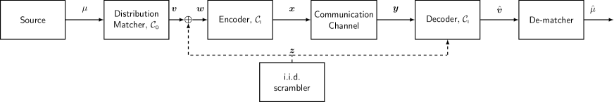
Figure 2: Modification of the system model of Figure 1, where an i.i.d. scrambler is introduced.

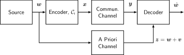
Figure 3: Equivalent parallel channel model.

III-A Belief Propagation Decoding

At the channel input, each codeword $\bm{c}$ is mapped onto $\{-1,+1\}^{n}$ via binary antipodal modulation, i.e., $x_{i}=1-2c_{i}$ for $i=1,\ldots,n$. With a slight abuse of notation, we will refer to the modulated codeword $\bm{x}$ as the codeword. We will also use $\mathcal{C}_{\scaleto{\mathsf{I}}{3.5pt}}$ and $\mathcal{C}$ to denote the modulated codebook of the inner code and of the overall code, respectively. We assume next that decoding is performed via belief propagation (BP) applied to the bipartite graph of the mother LDPC code. We initialize the BP decoder as follows. Let us denote by $L_{i}$ the $L$-value at the input of the $i$th VN. Moreover, define $\Delta=\ln[(1-\omega)/\omega]$. We set $L_{i}=\Delta$ is $i\leq h$, whereas we set $L_{i}=2y_{i-h}/\sigma^{2}$ if $i>h$. In other words, for the punctured VNs we provide prior information obtained from the marginal distribution of the CC code codeword $\bm{v}$, while for VNs associated with the codeword bits that are transmitted through the biAWGN channel, we input the corresponding channel log-likelihood ratios. The BP decoder output $\hat{\bm{v}}$ in then processed by the de-matcher [10], producing the estimate $\hat{\mu}$ of the transmitted message (see Figure 1). It is interesting to note that this decoder (proposed already in [1]) employs the same layered decoding architecture [14] adopted by PAS [7]: the BP decoder does not have any information on the outer CC constraints, and it exploits only the knowledge of the marginal distribution of the bits in $\bm{v}$.

III-B More on Decoding Metrics

We introduce next two decoding approaches which, albeit impractical, will be useful in the analysis of MN codes. We first consider the maximum likelihood (ML) decoder

$$\hat{\bm{x}}_{\scaleto{\mathsf{ML}}{3.5pt}}=\operatorname*{arg\,max}_{\bm{x}\in\mathcal{C}}p(\bm{y}|\bm{x})$$ (3)

where $p(\bm{y}|\bm{x})$ is the probability density of the biAWGN channel output $\bm{y}$ conditioned on the input $\bm{x}$. Note that the ML criterion (3) can be rephrased as

$$\hat{\bm{x}}_{\scaleto{\mathsf{ML}}{3.5pt}}=\operatorname*{arg\,max}_{\bm{x}\in\mathcal{C}_{\scaleto{\mathsf{I}}{3.5pt}}}p(\bm{y}|\bm{x}(\bm{v}))P(\bm{v}).$$ (4)

In (4), the dependency of $\bm{x}$ (inner encoder output) on $\bm{v}$ (inner encoder input) is emphasized. Note in particular that the search is over the inner code $\mathcal{C}_{\scaleto{\mathsf{I}}{3.5pt}}$, hence, over an enlarged set compared to (3): the overall code structure is conveyed by the prior $P(\bm{v})$ taking value $1/|\mathcal{C}_{\scaleto{\mathsf{O}}{3.5pt}}|$ if $\bm{v}\in\mathcal{C}_{\scaleto{\mathsf{O}}{3.5pt}}$, and taking value zero otherwise. Following the spirit of the BP decoder, which employs the marginal distribution of the bits composing $\bm{v}$ to bias the decoder operating over the bipartite graph of the mother code, we consider also a decoder that outputs

$$\hat{\bm{x}}_{\scaleto{\mathsf{MM}}{3.5pt}}=\operatorname*{arg\,max}_{\bm{x}\in\mathcal{C}_{\scaleto{\mathsf{I}}{3.5pt}}}p(\bm{y}|\bm{x}(\bm{v}))Q(\bm{v}).$$ (5)

where $Q(\bm{v})=\prod_{i=1}^{h}P(v_{i})$ denotes the product of the marginal distributions of the bits $v_{1},v_{2},\ldots,v_{h}$. The decoding metric adopted in (5) is clearly suboptimal compared with the one of (4). In fact, the term $Q(\bm{v})$ acts as a mismatched prior, yielding a nonzero probability also for $\bm{v}\notin\mathcal{C}_{\scaleto{\mathsf{O}}{3.5pt}}$. We refer to the decoding metric $p(\bm{y}|\bm{x}(\bm{v}))Q(\bm{v})$ as the mismatched metric.

III-C Equivalent Parallel Channel Model

The analysis of the scheme described in the previous sections presents some challenges. For example, being the code $\mathcal{C}$ nonlinear, the block error probability under (3)–(4) will depend upon the transmitted codeword. This hinders the use of a reference codeword to compute bounds on the block error probability. A similar issue arises when attempting a DE evolution analysis under BP decoding, where typically the allzero codeword is used as reference. The issue can be circumvented by resorting to alternative communication models that can be proved to be equivalent to the one depicted in Figure 1 [15, 5]. Consider first the scheme depicted in Figure 2, where a scrambling block is introduced. The block generates a sequence $\bm{z}=(z_{1},z_{2},\ldots,z_{h})$ where each element is picked independently and uniformly at random in $\{0,1\}$. The sequence $\bm{z}$ is then added (in $\mathbbmss{F}_{\!\scaleto{\mathsf{2}}{3.5pt}}$) to $\bm{v}$ prior to encoding with $\mathcal{C}_{\scaleto{\mathsf{I}}{3.5pt}}$. The same sequence is made available to the decoder. Considering either (3) or (4), and owing to the symmetry of the biAWGN channel, we observe that the presence of the scrambler is irrelevant to the analysis of the error probability, since the addition of $\bm{z}$ at the transmitter side can be compensated at the decoder by computing first $\bm{b}=\bm{z}\bm{G}$, and then flipping the sign of the observations $y_{i}$ for all $i\in\mathrm{supp}(\bm{b})$. The model of Figure 2 admits an equivalent model, provided in Figure 3: here, an i.i.d. uniform binary source generates an $h$-bits vector $\bm{w}$, which is encoded via $\mathcal{C}_{\scaleto{\mathsf{I}}{3.5pt}}$ yielding a codeword $\bm{x}$ that is transmitted through the biAWGN channel. The decoder obtains also an observation of $\bm{w}$ via a so-called a priori channel. The a priori channel adds (in $\mathbbmss{F}_{\!\scaleto{\mathsf{2}}{3.5pt}}$) a weight-$\omega h$ binary vector $\bm{v}$ to $\bm{w}$, were $\bm{v}$ is picked uniformly at random in $\mathcal{C}_{\scaleto{\mathsf{O}}{3.5pt}}$, resulting in the observation $\bm{z}$. Upon observing $\bm{y}$ and $\bm{z}$, the decoder produces a decision on $\bm{w}$, or, equivalently, a decision on $\bm{v}$ since $\bm{w}=\bm{v}+\bm{z}$. ML decoding will produce

$$\hat{\bm{x}}_{\scaleto{\mathsf{ML}}{3.5pt}}=\operatorname*{arg\,max}_{\bm{x}\in\mathcal{C}_{\scaleto{\mathsf{I}}{3.5pt}}}p(\bm{y}|\bm{x}(\bm{w}))P(\bm{z}|\bm{w})$$ (6)

where $P(\bm{z}|\bm{w})=1/|\mathcal{C}_{\scaleto{\mathsf{O}}{3.5pt}}|$ if $(\bm{z}-\bm{w})\in\mathcal{C}_{\scaleto{\mathsf{O}}{3.5pt}}$, and $P(\bm{z}|\bm{w})=0$ otherwise. The decoding problem can be immediately recognized to be equivalent to the one in (4). The decoder may also resort to a mismatched model for the a priori channel, treating it as a binary symmetric channel (BSC) with crossover probability $\omega$ and resulting in

$$\hat{\bm{x}}_{\scaleto{\mathsf{MM}}{3.5pt}}=\operatorname*{arg\,max}_{\bm{x}\in\mathcal{C}_{\scaleto{\mathsf{I}}{3.5pt}}}p(\bm{y}|\bm{x}(\bm{w}))Q(\bm{z}|\bm{w})$$ (7)

where $Q(\bm{z}|\bm{w})=\prod_{i=1}^{h}P(z_{i}|w_{i})$, i.e., the solution of (7) is equivalent to the solution of (5). We refer to the model of Figure 3 as the equivalent parallel channel (EPC) model. The convenience of the EPC model stems from the fact that, owing to the symmetry of the communication and of the a priori channels, and to the linearity of the code $\mathcal{C}_{\scaleto{\mathsf{I}}{3.5pt}}$, the error probability is independent on $\bm{w}$: we can analyze the error probability of the scheme of Figure 3 by fixing as reference the allzero codeword. The resulting analysis will characterize exactly the performance of the original scheme of Figure 1.

IV Density Evolution Analysis

Protograph-based MN code ensembles can be analyzed via DE by resorting to the EPC model introduced in Section III-C. The analysis shares several commonalities with the DE of LDPC code ensembles designed for joint source and channel coding [5]. We performed the analysis both via quantized DE [13], as well as by means of the Gaussian approximation in the form of PEXIT analysis [11, 12]. In either case, with reference to the EPC model, we replaced the a priori channel (that introduces a constant number of errors $\omega h$ in $\bm{z}$) with a BSC with crossover probability $\omega$. The choice is justified by observing that, as $h$ (and $n$) grows large, the fraction of errors introduced by the BSC concentrates around $\omega$. We describe next how to perform the PEXIT analysis, following the steps in [12]. Denote by $C_{\scaleto{\mathsf{BSC}}{3.5pt}}(\omega)$ the capacity of a BSC with crossover probability $\omega$, and by $C_{\scaleto{\mathsf{AWGN}}{3.5pt}}(E_{s}/N_{0})$ the capacity of a biAWGN channel with SNR $E_{s}/N_{0}$. The PEXIT analysis is initialized by setting the mutual information (MI) at the input of type-$i$ VNs, $i=1,\ldots,h_{0}$, to $C_{\scaleto{\mathsf{BSC}}{3.5pt}}(\omega)$, whereas for $i=h_{0}+1,\ldots,h_{0}+n_{0}$ the MI at the input of type-$i$ VNs is initialized to $C_{\scaleto{\mathsf{AWGN}}{3.5pt}}(E_{s}/N_{0})$. The analysis in then carried out via the recursions provided in [12], and it allows to determine (for fixed $\omega$) the iterative decoding threshold over the biAWGN channel, that is the minimum $E_{s}/N_{0}$ for which the MI values tracked by the PEXIT analysis converge to $1$. We denote the threshold value as $\gamma^{\star}(R)$, where we emphasize the dependency on $R$ (and, hence, on $\omega$). Due to the faster computations entailed by the PEXIT analysis with respect to quantized DE, PEXIT analysis will be used for protograph optimization, while quantized DE will be used to verify the accuracy of the thresholds computed for the designed protographs.

The threshold $\gamma^{\star}$ can be used as target measure to be minimized in the design of protographs. In particular, suppose we are interested in finding an inner mother code protograph that allows to operate close to capacity over a range $\left[\underline{R},\overline{R}\right]$ of rates $R$, i.e., over a range $\left[\underline{\omega},\overline{\omega}\right]$ of values of $\omega$. Fix the protograph parameters $h_{0},n_{0}$. By doing so, the inner code rate $R_{\scaleto{\mathsf{I}}{3.5pt}}$ is fixed. A set of target rates $\mathcal{R}\subset\left[\underline{R},\overline{R}\right]$ is selected. For each target rate $R\in\mathcal{R}$ we can derive the rate of the DM as $R_{\scaleto{\mathsf{O}}{3.5pt}}=R/R_{\scaleto{\mathsf{I}}{3.5pt}}$, out of which the DM parameter $\omega$ is obtained. Given a protograph $\mathcal{P}$ we define the worst-case loss (WCL)

$$\Delta(\mathcal{P}):=\max_{R\in\mathcal{R}}\left[\gamma^{\star}(R)-C_{\scaleto{\mathsf{AWGN}}{3.5pt}}^{-1}(R)\right]$$ (8)

that is the maximum gap between the protograph iterative decoding threshold and the biAWGN Shannon limit for the rates in $\mathcal{R}$. A search for the protograph with parameters $h_{0},n_{0}$ that minimizes the WCL in (8) can be carried out, for example, via differential evolution [16]. We provide next some examples of application to the design of protograph-based MN code ensemble families addressing different rate regimes. In all examples, the search space was limited by setting the maximum number of parallel edges between protograph VN/CN pairs (i.e., value of the base matrix elements) to $3$.

Example 1.

Consider a code rate range $[0.1,0.5]$. An MN code family addressing this range can be derived from an inner $R_{\scaleto{\mathsf{I}}{3.5pt}}=1/2$ code, i.e., the mother code has rate $R_{\scaleto{\mathsf{IM}}{3.5pt}}=1/3$. We search for protographs with $6$ VNs and $4$ CNs, minimizing the WCL over $\mathcal{R}=\{0.1,0.3,0.5\}$. We obtain the base matrix

$$\bm{B}_{1/2} =\left(\begin{array}[]{cc|cccc}1&0&1&1&0&0\\ 0&1&0&3&0&1\\ 2&0&1&1&1&0\\ 1&2&1&2&0&0\end{array}\right).$$ (13)

where the first two columns are associated with punctured VNs. The decoding thresholds for the code ensemble defined by $\bm{B}_{1/2}$ are provided in Table I for various rates. The values are computed with both quantized DE and PEXIT analysis. The results confirm the accuracy of the latter, with thresholds that are within $0.05$ dB from the quantized DE ones for rates in the ranging from $0.3$ to $0.5$. The accuracy reduces for the lowest rates, however still yielding acceptable estimates.

TABLE I: Thresholds (dB) computed by quantized DE and by PEXIT for different overall code rate $R$

$R$	$0.5$	$0.4$	$0.3$	$0.2$	$0.1$
$\gamma^{\star}$ dB (quant. DE)	$-2.01$	$-3.38$	$-5.02$	$-7.00$	$-10.32$
$\gamma^{\star}$ dB (PEXIT)	$-2.06$	$-3.42$	$-5.05$	$-7.14$	$-10.49$

Example 2.

Consider a code rate range $[0.1,0.666]$. An MN code family addressing this range can be derived from an inner $R_{\scaleto{\mathsf{I}}{3.5pt}}=2/3$ code. Accordingly, fix the base matrix to be a $3\times 5$ matrix. We search for protographs minimizing the WCL over $\mathcal{R}=\{0.1,0.3,0.666\}$. We obtain the base matrix

$$\bm{B}_{2/3} =\left(\begin{array}[]{cc|ccc}1&0&0&3&1\\ 1&1&0&3&0\\ 1&2&2&1&0\end{array}\right).$$ (17)

Remarkably, the iterative decoding thresholds for both ensembles of Examples 1 and 2 (displayed in Figure 4) are within $1$ dB from the Shannon limit over a wide range of rates.

V Finite Length Performance Analysis

In this section, we provide numerical results on finite-length constructions of protograph MN codes. We complement Monte Carlo simulation results with an error floor analysis based on the union bound (UB) on the block error probability. In particular, we analyze mismatched decoding as defined in (7). This choice follows the observation that the BP decoder does not exploit the joint p.m.f. $P(\bm{v})$, but rather the marginal distribution $P(v_{i})$ for all $i=1,\ldots,h$. By resorting to the EPC setting, the derivation of bounds on the error probability under (6) reduces to the analysis of the error probability under (7). We first derive the pairwise error probability

$$\mathsf{PEP}(\bm{x}^{\prime})=\mathsf{P}\big{[}\,p(\bm{Y}|\bm{x})Q(\bm{Z}|\bm{w})\leq p(\bm{Y}|\bm{x}^{\prime})Q(\bm{Z}|\bm{w}^{\prime})\,\big{]}.$$ (18)

In (18), the codeword transmitted over the communication channel is $\bm{x}$, and it is the result of the encoding of $\bm{w}$, where the vector $\bm{w}$ is transmitted over the a priori channel. The competing codeword is $\bm{x}^{\prime}$, and it is the result of the encoding of $\bm{w}^{\prime}$. Note that in (18) ties are broken in favor of the competing codeword. Owing to the symmetry of the communication and a priori channels, and to the linearity of $\mathcal{C}_{\scaleto{\mathsf{I}}{3.5pt}}$, we assume without loss of generality that $\bm{w}=(0,0,\ldots,0)$ and hence $\bm{x}=(+1,+1,\ldots,+1)$. Conditioned on $\bm{X}=\bm{x}$ and $\bm{W}=\bm{w}$, $\bm{Z}$ is uniformly distributed over the set of $h$-bit sequences with Hamming weight $\omega h$, whereas $Y_{1},Y_{2},\ldots,Y_{n}$ are i.i.d. $\sim\mathcal{N}(+1,\sigma^{2})$. We can rewrite (18) as

$$\mathsf{PEP}(\bm{x}^{\prime}) =\mathsf{P}\!\left[\sum_{i=1}^{n}\ln\frac{p(Y_{i}|x_{i})}{p(Y_{i}|x_{i}^{\prime})}\leq\sum_{i=1}^{h}\ln\frac{Q(Z_{i}|w_{i}^{\prime})}{Q(Z_{i}|w_{i})}\right]$$ (19)

$$=\mathsf{P}\!\left[\textstyle\sum_{i\in\mathcal{D}(\bm{x}^{\prime})}L_{i}\leq-\sum_{i\in\mathcal{D}(\bm{w}^{\prime})}T_{i}\right].$$ (20)

In (20), $\mathcal{D}(\bm{x}^{\prime})=\{i|x_{i}^{\prime}\neq x_{i}\}$, $\mathcal{D}(\bm{w}^{\prime})=\{i|w_{i}^{\prime}\neq w_{i}\}$, whereas $L_{i}:=\ln[p(Y_{i}|+1)/p(Y_{i}|-1)]$ and $T_{i}:=\ln[p(Z_{i}|0)/p(Z_{i}|1)]$. Denote by $L=\sum_{i\in\mathcal{D}(\bm{x}^{\prime})}L_{i}$ and by $T=\sum_{i\in\mathcal{D}(\bm{w}^{\prime})}T_{i}$. Moreover, let $\delta_{1}=d_{\scaleto{\mathsf{H}}{3.5pt}}(\bm{w},\bm{w}^{\prime})$ and $\delta_{2}=d_{\scaleto{\mathsf{H}}{3.5pt}}(\bm{x},\bm{x}^{\prime})$. Conditioned on $\bm{X}=\bm{x}$ and $\bm{W}=\bm{w}$, we have that $L\sim\mathcal{N}(2\delta_{2}/\sigma^{2},4\delta_{2}/\sigma^{2})$. Recalling $\Delta=\ln[(1-\omega)/\omega]$, we have that $T_{i}=\Delta$ if $Z_{i}=0$, whereas $T_{i}=-\Delta$ if $Z_{i}=1$, i.e.,

$$T=(\delta_{1}-E)\Delta-E\Delta=\delta_{1}-2E\Delta$$

where $E$ follows an hypergeometric distribution with parameters $(h,\omega h,\delta_{1})$. After a few simple manipulations, we obtain

$$\mathsf{PEP}(\bm{x}^{\prime})=\mathsf{E}\!\left[Q\left(\frac{2\delta_{2}/\sigma^{2}+\delta_{1}-2E\Delta}{2\sqrt{\delta_{2}}/\sigma}\right)\right]$$ (21)

where $Q(x)$ is the well-known Gaussian $Q$-function. By observing that $\mathsf{PEP}(\bm{x}^{\prime})$ depends on $\bm{x}^{\prime}$ only through its Hamming distance from $\bm{x}$, and on the Hamming distance between the corresponding information sequence $\bm{w}^{\prime}$ and $\bm{w}$, we can upper bound the block error probability under (7) as

$$P_{B} \leq\sum_{\delta_{1}=1}^{h}\sum_{\delta_{2}=1}^{n}A^{\scaleto{\mathsf{IO}}{3.5pt}}_{\delta_{1},\delta_{2}}\mathsf{E}\!\left[Q\left(\frac{2\delta_{2}/\sigma^{2}+\delta_{1}-2E\Delta}{2\sqrt{\delta_{2}}/\sigma}\right)\right]$$ (22)

where $A^{\scaleto{\mathsf{IO}}{3.5pt}}_{\delta_{1},\delta_{2}}$ is the input-output weight enumerator of $\mathcal{C}_{\scaleto{\mathsf{I}}{3.5pt}}$. At large SNRs, (22) can be approximated by truncating the summation to the dominant term $A^{\scaleto{\mathsf{IO}}{3.5pt}}_{\delta^{\star}_{1},\delta^{\star}_{2}}$, yielding

$$P_{B}\approx A^{\scaleto{\mathsf{IO}}{3.5pt}}_{\delta^{\star}_{1},\delta^{\star}_{2}}\mathsf{E}\!\left[Q\left(\frac{2\delta^{\star}_{2}/\sigma^{2}+\delta^{\star}_{1}-2E\Delta}{2\sqrt{\delta^{\star}_{2}}/\sigma}\right)\right].$$ (23)

A possible strategy to identify the dominant term $A^{\scaleto{\mathsf{IO}}{3.5pt}}_{\delta^{\star}_{1},\delta^{\star}_{2}}$ can be to enumerate low-weight codewords of $\mathcal{C}_{\scaleto{\mathsf{I}}{3.5pt}}$ (e.g., via the algorithm proposed in [17]). Once a sufficient number of low-weight codewords is collected, their contribution to the error probability can be measured via (21).

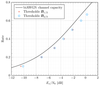
Figure 4: Iterative decoding thresholds computed for the MN code ensembles defined by the base matrices described in Example 1 and in Example 2.

Figure 5 reports simulation results for a length-$1200$ MN code family, for different rates $R\in[0.1,0.5]$. The base matrix of $\mathcal{C}_{\scaleto{\mathsf{IM}}{3.5pt}}$ is $\bm{B}_{1/2}$. The protograph was lifted through a circulant version of the progressive edge growth (PEG) algorithm [18]. The truncated union bounds provide an excellent prediction of the frame error rate (FER) at large SNRs. Interestingly, the TUBs indicate at large SNR a diminishing return in coding gain when the rate of the outer CC is reduced, whereas the coding gains at moderate FER are more sizeable.

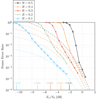
Figure 5: FER vs. $E_{s}/N_{0}$ dB for length-$1200$ protograph MN code with inner mother code base matrix $\bm{B}_{1/2}$ and code rate range $[0.1,0.5]$. The TUB of the block error probability for each rate is provided (dashed lines) as well as the corresponding iterative decoding thresholds.

References

- [1] D. MacKay, “Good error-correcting codes based on very sparse matrices,” IEEE Trans. Inf. Theory, vol. 45, no. 2, pp. 399–431, Mar. 1999.
- [2] R. Gallager, “Low-density parity-check codes,” Ph.D. dissertation, Massachusetts Institute of Technology, Cambridge, MA, USA, 1963.
- [3] T. Richardson and R. Urbanke, Modern coding theory. Cambridge University Press, 2008.
- [4] M. J. Wainwright and E. Martinian, “Low-density graph codes that are optimal for binning and coding with side information,” IEEE Trans. Inf. Theory, vol. 55, no. 3, pp. 1061–1079, Mar. 2009.
- [5] M. Fresia, F. Perez-Cruz, H. V. Poor, and S. Verdu, “Joint source and channel coding,” IEEE Signal Process. Mag., vol. 27, no. 6, pp. 104–113, Nov. 2010.
- [6] A. Morello and V. Mignone, “DVB-S2: The second generation standard for satellite broad-band services,” Proc. IEEE, vol. 94, no. 1, pp. 210–227, Jan. 2006.
- [7] G. Böcherer, F. Steiner, and P. Schulte, “Bandwidth efficient and rate-matched low-density parity-check coded modulation,” IEEE Trans. Commun., vol. 63, no. 12, pp. 4651–4665, Dec. 2015.
- [8] F. Buchali, F. Steiner, G. Böcherer, L. Schmalen, P. Schulte, and W. Idler, “Rate adaptation and reach increase by probabilistically shaped -QAM: An experimental demonstration,” IEEE/OSA J. Lightw. Technol., vol. 34, no. 7, pp. 1599–1609, Apr. 2016.
- [9] J. Thorpe, “Low-density parity-check (LDPC) codes constructed from protographs,” NASA JPL, IPN Progr. Rep. 42-154, Aug. 2003.
- [10] P. Schulte and G. Böcherer, “Constant composition distribution matching,” IEEE Trans. Inf. Theory, vol. 62, no. 1, pp. 430–434, Jan. 2016.
- [11] S. ten Brink, “Convergence behavior of iteratively decoded parallel concatenated codes,” IEEE Trans. Commun., vol. 49, no. 10, pp. 1727–1737, Oct. 2001.
- [12] G. Liva and M. Chiani, “Protograph LDPC codes design based on EXIT analysis,” in Proc. IEEE Global Telecommun. Conf., Nov. 2007.
- [13] T. Richardson and R. Urbanke, “The capacity of low-density parity-check codes under message-passing decoding,” IEEE Trans. Inf. Theory, vol. 47, no. 2, pp. 599–618, Feb. 2001.
- [14] G. Böcherer, “Achievable rates for probabilistic shaping,” arXiv preprint arXiv:1707.01134, 2017.
- [15] A. Wyner, “Recent results in the Shannon theory,” IEEE Trans. Inf. Theory, vol. 20, no. 1, pp. 2–10, Jan. 1974.
- [16] A. Shokrollahi and R. Storn, “Design of efficient erasure codes with differential evolution,” in Differential Evolution. Springer, 2005.
- [17] X.-Y. Hu, M. P. C. Fossorier, and E. Eleftheriou, “On the computation of the minimum distance of low-density parity-check codes,” in Proc. IEEE Int. Conf. Commun., Jun. 2004.
- [18] X.-Y. Hu, E. Eleftheriou, and D. Arnold, “Regular and irregular progressive edge-growth Tanner graphs,” IEEE Trans. Inf. Theory, vol. 51, no. 1, pp. 386–398, Jan. 2005.