A strongly conservative hybridizable discontinuous Galerkin method for the coupled time-dependent Navier–Stokes and Darcy problem

Abstract

We present a strongly conservative and pressure-robust hybridizable discontinuous Galerkin method for the coupled time-dependent Navier–Stokes and Darcy problem. We show existence and uniqueness of a solution and present an optimal a priori error analysis for the fully discrete problem when using Backward Euler time stepping. The theoretical results are verified by numerical examples.

1 Introduction

In this paper we present an analysis of a hybridizable discontinuous Galerkin (HDG) method for the coupled Navier–Stokes and Darcy equations that model surface/subsurface flow. While various conforming and nonconforming finite element methods have been studied for the stationary Navier–Stokes and Darcy problem, see for example [3, 13, 14, 18, 19, 22, 23], the literature on numerical methods for the time-dependent problem is limited. The first numerical methods for the time-dependent problem were studied in [7, 8]. To simplify the analysis, however, these papers included inertia effects in the balance of forces at the interface. Existence and uniqueness of a weak solution to the physically more relevant model, without inertia effects on the interface, was proven in [9], while convergence of a discontinuous Galerkin method for this model was proven in [12]. Conforming methods for the transient problem have been studied in [25, 43].

The aforementioned papers for the time-dependent Navier–Stokes and Darcy problem have in common that they consider the primal form of the Darcy problem. In contrast, we consider the mixed form of the Darcy problem as this facilitates the formulation of a strongly conservative discretization, i.e., a discretization that is mass conserving in the sense of $H(\text{div};\Omega)$ where the velocity is globally $H(\text{div};\Omega)$-conforming and, in the absence of sources and sinks, pointwise divergence-free on the elements [28]. In particular, we consider an HDG method [16] that is based on the HDG method for the Navier–Stokes equations [35] and a hybridized formulation of the mixed form of the Darcy problem [2], although nonconforming formulations based on other strongly conservative discretizations, for example, [15, 21, 31, 41], are possible.

Previously, we proved pressure-robustness of strongly conservative HDG methods for the Stokes/Darcy [11] and stationary Navier–Stokes/Darcy [6] problems, leading to a priori error estimates for the velocity that do not depend on the best approximation of the pressure scaled by the inverse of the viscosity (see [27, 32] for a review of other pressure-robust discretizations). Using Backward Euler time stepping we now show existence and uniqueness of a solution and derive an a priori error estimate to the fully-discrete time-dependent problem. Compared to previous work on the time-dependent Navier–Stokes/Darcy problem [7, 8, 9, 12, 25, 43], the novel contributions of this work is therefore the introduction and analysis of a strongly conservative HDG discretization and an a priori error estimate for the velocity that is independent of pressure.

The remainder of this paper is organized as follows. We present the time-dependent Navier–Stokes/Darcy problem in section 2 and its HDG discretization in section 3. Consistency and well-posedness of the discrete problem are shown in section 4 while a priori error estimates are proven in section 5. We end this paper with numerical examples in section 6 and conclusions in section 7.

2 The Navier–Stokes and Darcy problem

We consider the time-dependent incompressible Navier–Stokes equations coupled to the Darcy equations on a polyhedral domain $\Omega$ in $\mathbb{R}^{\dim}$, $\dim=2,3$, and on the time interval $J=(0,T)$. The domain is partitioned into two non-overlapping subdomains $\Omega^{s}$ and $\Omega^{d}$ such that $\Omega=\Omega^{s}\cup\Omega^{d}$, $\Omega^{s}\cap\Omega^{d}=\emptyset$, and $\Gamma^{I}\mathrel{\mathop{\mathchar 58\relax}}=\partial\Omega^{s}\cap\partial\Omega^{d}$. The boundary of the domain $\partial\Omega$ and the interface $\Gamma^{I}$ are assumed to be Lipschitz polyhedral. We define $\Gamma^{s}$ and $\Gamma^{d}$ to be the exterior boundaries of $\Omega^{s}$ and $\Omega^{d}$, respectively. We partition $\Gamma^{d}\mathrel{\mathop{\mathchar 58\relax}}=\Gamma_{N}^{d}\cup\Gamma_{D}^{d}$, with $\Gamma_{N}^{d}\cap\Gamma_{D}^{d}=\emptyset$ and $|\Gamma_{N}^{d}|>0$ and $|\Gamma_{D}^{d}|>0$, and denote the outward unit normal on $\Gamma^{j}$ to $\Omega^{j}$ ($j=s,d$) by $n$.

The Navier–Stokes equations are given by

$$\partial_{t}u^{s}+\nabla\cdot(u^{s}\otimes u^{s})+\nabla p^{s}-\nabla\cdot(2\mu\varepsilon(u^{s})) =f^{s} \text{ in }\Omega^{s}\times J,$$ (1a)

$$\nabla\cdot u^{s} =0 \text{ in }\Omega^{s}\times J,$$ (1b)

where $u^{s}\mathrel{\mathop{\mathchar 58\relax}}\Omega^{s}\times J\to\mathbb{R}^{\dim}$ is the velocity in $\Omega^{s}$, $p^{s}\mathrel{\mathop{\mathchar 58\relax}}\Omega^{s}\times J\to\mathbb{R}^{\dim}$ is the pressure in $\Omega^{s}$, $\varepsilon(w)=\tfrac{1}{2}(\nabla w+(\nabla w)^{T})$, $\mu>0$ is the constant fluid viscosity, and $f^{s}\mathrel{\mathop{\mathchar 58\relax}}\Omega^{s}\times J\to\mathbb{R}^{\dim}$ is a body force. In $\Omega^{d}$ the Darcy equations are given by:

$$\mu\kappa^{-1}u^{d}+\nabla p^{d} =0 \text{ in }\Omega^{d}\times J,$$ (2a)

$$-\nabla\cdot u^{d} =f^{d} \text{ in }\Omega^{d}\times J,$$ (2b)

where $u^{d}\mathrel{\mathop{\mathchar 58\relax}}\Omega^{d}\times J\to\mathbb{R}^{\dim}$ is the fluid velocity in $\Omega^{d}$, $p^{d}\mathrel{\mathop{\mathchar 58\relax}}\Omega^{d}\times J\to\mathbb{R}$ is the piezometric head in $\Omega^{d}$, and $\kappa>0$ is the permeability constant. The Navier–Stokes equations are coupled to the Darcy equations by the following interface conditions

$$u^{s}\cdot n =u^{d}\cdot n \text{ on }\Gamma^{I}\times J,$$ (3a)

$$-2\mu(\varepsilon(u^{s})n)^{t} =\alpha\mu\kappa^{-1/2}(u^{s})^{t} \text{ on }\Gamma^{I}\times J,$$ (3b)

$$(p^{s}n-2\mu\varepsilon(u^{s})n)\cdot n =p^{d} \text{ on }\Gamma^{I}\times J,$$ (3c)

where $n$ is the unit normal vector on $\Gamma^{I}$ pointing from $\Omega^{s}$ to $\Omega^{d}$, $(v)^{t}\mathrel{\mathop{\mathchar 58\relax}}=v-(v\cdot n)n$ is the tangential component of a vector $v$, and $\alpha>0$ is an experimentally determined dimensionless constant. Note that eq. 3a ensures continuity of the normal component of the velocity across the interface, eq. 3b is the Beavers–Joseph–Saffman law [4, 38], and eq. 3c is a balance of forces. We assume the following initial and boundary conditions:

$$u^{s}(x,0) =u_{0}(x) \text{ in }\Omega^{s},$$ (4a)

$$u^{s} =0 \text{ on }\Gamma^{s}\times J,$$ (4b)

$$u^{d}\cdot n =0 \text{ on }\Gamma^{d}_{N}\times J,$$ (4c)

$$p^{d} =0 \text{ on }\Gamma^{d}_{D}\times J,$$ (4d)

where $u_{0}\mathrel{\mathop{\mathchar 58\relax}}\Omega^{s}\to\mathbb{R}^{\dim}$ is a solenoidal initial velocity field. We close this section by introducing $u\mathrel{\mathop{\mathchar 58\relax}}\Omega\times J\to\mathbb{R}^{\dim}$ and $p\mathrel{\mathop{\mathchar 58\relax}}\Omega\times J\to\mathbb{R}$ to be the functions such that $u|_{\Omega^{j}}=u^{j}$ and $p|_{\Omega^{j}}=p^{j}$ for $j=s,d$.

3 The HDG method

3.1 Notation

Let $j=s,d$. We denote by $\mathcal{T}_{h}^{j}=\mathinner{\{K\}}$ a conforming triangulation of $\Omega^{j}$ of shape-regular simplices $K$. We assume that $\mathcal{T}_{h}=\mathcal{T}_{h}^{s}\cup\mathcal{T}_{h}^{d}$ is a matching simplicial mesh, i.e., $\mathcal{T}_{h}^{s}$ and $\mathcal{T}_{h}^{d}$ match at the interface. We denote by $h_{K}$ the diameter of $K\in\mathcal{T}_{h}$ and define the meshsize as $h\mathrel{\mathop{\mathchar 58\relax}}=\max_{K\in\mathcal{T}_{h}}h_{K}$. A face $F$ is an interior face if for two elements $K^{+}$ and $K^{-}$ in $\mathcal{T}_{h}$, $F=\partial K^{+}\cap\partial K^{-}$, and a boundary face if $F\in\partial K$ lies on the boundary $\partial\Omega$. The set of all facets in $\overline{\Omega}$ and $\overline{\Omega}^{j}$ are denoted by, respectively, $\mathcal{F}_{h}$ and $\mathcal{F}_{h}^{j}$, while the set of all facets on the interface $\Gamma^{I}$ is denoted by $\mathcal{F}_{h}^{I}$. The set of all facets on $\Gamma^{j}$ are denoted by $\mathcal{F}_{h}^{B,j}$ while the set of all facets interior to $\Omega^{j}$ are denoted by $\mathcal{F}_{h}^{int,j}$. The sets of facets on $\Gamma_{N}^{d}$ and $\Gamma_{D}^{d}$ are denoted by, respectively, $\mathcal{F}_{h}^{N,d}$ and $\mathcal{F}_{h}^{D,d}$. By $\Gamma_{0}$ and $\Gamma_{0}^{j}$ we denote the union of facets in $\overline{\Omega}$ and $\overline{\Omega}^{j}$. The outward unit normal vector on $\partial K$ for any element $K\in\mathcal{T}_{h}^{j}$ is denoted by $n^{j}$. On the interface $\Gamma^{I}$, $n=n^{s}=-n^{d}$. We will drop the superscript $j$ if the definition of the outward unit normal vector is clear.

We partition the time interval $J$ into $N$ equal intervals of length $\Delta t=T/N$. We define $t^{n}\mathrel{\mathop{\mathchar 58\relax}}=n\Delta t$ for $n=0,\ldots,N$ and note that $t^{0}=0$ and $t^{N}=T$. A function $f$ evaluated at $t=t^{n}$ will be denoted by $f^{n}\mathrel{\mathop{\mathchar 58\relax}}=f(t^{n})$. Furthermore, we define $\delta f^{n+1}=f^{n+1}-f^{n}$ and $d_{t}f^{n+1}=\delta f^{n+1}/\Delta t=(f^{n+1}-f^{n})/\Delta t$.

Denoting by $P_{m}(D)$ the space of polynomials of total degree $m$ on a domain $D$, we define the following finite element spaces for the velocity approximation:

$$\begin{split}X_{h}&\mathrel{\mathop{\mathchar 58\relax}}=\mathinner{\bigl{\{}v_{h}\in\mathinner{[L^{2}(\Omega)]}^{\dim}\mathrel{\mathop{\mathchar 58\relax}}\ v_{h}\in\mathinner{[P_{k}(K)]}^{\dim},\ \forall\ K\in\mathcal{T}\bigr{\}}},\\ X_{h}^{j}&\mathrel{\mathop{\mathchar 58\relax}}=\mathinner{\bigl{\{}v_{h}\in\mathinner{[L^{2}(\Omega^{j})]}^{\dim}\mathrel{\mathop{\mathchar 58\relax}}\ v_{h}\in\mathinner{[P_{k}(K)]}^{\dim},\ \forall\ K\in\mathcal{T}^{j}\bigr{\}}},\quad j=s,d,\\ \bar{X}_{h}&\mathrel{\mathop{\mathchar 58\relax}}=\mathinner{\bigl{\{}\bar{v}_{h}\in\mathinner{[L^{2}(\Gamma_{0}^{s})]}^{\dim}\mathrel{\mathop{\mathchar 58\relax}}\ \bar{v}_{h}\in\mathinner{[P_{k}(F)]}^{\dim}\ \forall\ F\in\mathcal{F}^{s},\ \bar{v}_{h}=0\text{ on }\Gamma^{s}\bigr{\}}}.\end{split}$$

For notational purposes, we write $\boldsymbol{v}_{h}=(v_{h},\bar{v}_{h})\in\boldsymbol{X}_{h}\mathrel{\mathop{\mathchar 58\relax}}=X_{h}\times\bar{X}_{h}$ and $\boldsymbol{v}_{h}^{s}=(v_{h}^{s},\bar{v}_{h})\in\boldsymbol{X}_{h}^{s}\mathrel{\mathop{\mathchar 58\relax}}=X_{h}^{s}\times\bar{X}_{h}$. Furthermore, for the pressure approximation we define the finite element spaces

$$\begin{split}Q_{h}&\mathrel{\mathop{\mathchar 58\relax}}=\mathinner{\bigl{\{}q_{h}\in L^{2}(\Omega)\mathrel{\mathop{\mathchar 58\relax}}\ q_{h}\in P_{k-1}(K),\ \forall\ K\in\mathcal{T}\bigr{\}}},\\ Q_{h}^{j}&\mathrel{\mathop{\mathchar 58\relax}}=\mathinner{\bigl{\{}q_{h}\in L^{2}(\Omega^{j})\mathrel{\mathop{\mathchar 58\relax}}\ q_{h}\in P_{k-1}(K),\ \forall\ K\in\mathcal{T}^{j}\bigr{\}}},\quad j=s,d,\\ \bar{Q}_{h}^{s}&\mathrel{\mathop{\mathchar 58\relax}}=\mathinner{\bigl{\{}\bar{q}_{h}^{s}\in L^{2}(\Gamma_{0}^{s})\mathrel{\mathop{\mathchar 58\relax}}\ \bar{q}_{h}^{s}\in P_{k}(F)\ \forall\ F\in\mathcal{F}^{s}\bigr{\}}},\\ \bar{Q}_{h}^{d}&\mathrel{\mathop{\mathchar 58\relax}}=\mathinner{\bigl{\{}\bar{q}_{h}^{d}\in L^{2}(\Gamma_{0}^{d})\mathrel{\mathop{\mathchar 58\relax}}\ \bar{q}_{h}^{d}\in P_{k}(F)\ \forall\ F\in\mathcal{F}^{d},\ \bar{q}_{h}^{d}=0\text{ on }\Gamma_{D}^{d}\bigr{\}}}.\end{split}$$

We write $\boldsymbol{q}_{h}=(q_{h},\bar{q}_{h}^{s},\bar{q}_{h}^{d})\in\boldsymbol{Q}_{h}\mathrel{\mathop{\mathchar 58\relax}}=Q_{h}\times\bar{Q}_{h}^{s}\times\bar{Q}_{h}^{d}$ and $\boldsymbol{q}_{h}^{j}=(q_{h},\bar{q}_{h}^{j})\in\boldsymbol{Q}_{h}^{j}\mathrel{\mathop{\mathchar 58\relax}}=Q_{h}^{j}\times\bar{Q}_{h}^{j}$.

For scalar functions $p$ and $q$, we define

$$(p,q)_{K} \mathrel{\mathop{\mathchar 58\relax}}=\int_{K}pq\operatorname{d\!}x,\quad\forall K\in\mathcal{T}_{h}, \langle p,q\rangle_{\partial K} \mathrel{\mathop{\mathchar 58\relax}}=\int_{\partial K}pq\operatorname{d\!}s,\quad\forall K\in\mathcal{T}_{h},$$

$$\langle p,q\rangle_{F} \mathrel{\mathop{\mathchar 58\relax}}=\int_{F}pq\operatorname{d\!}s,\quad F\subset\partial K,\ \forall K\in\mathcal{T}_{h}, (p,q)_{\Omega^{j}} \mathrel{\mathop{\mathchar 58\relax}}=\sum_{K\in\mathcal{T}_{h}^{j}}(p,q)_{K},\quad j=s,d,$$

$$\langle p,q\rangle_{\partial\mathcal{T}_{h}^{j}} \mathrel{\mathop{\mathchar 58\relax}}=\sum_{K\in\mathcal{T}_{h}^{j}}\langle p,q\rangle_{\partial K},\quad j=s,d, (p,q)_{\Omega} \mathrel{\mathop{\mathchar 58\relax}}=\sum_{K\in\mathcal{T}_{h}}\int_{K}pq\operatorname{d\!}x,$$

$$\langle p,q\rangle_{\partial\mathcal{T}_{h}} \mathrel{\mathop{\mathchar 58\relax}}=\sum_{K\in\mathcal{T}_{h}}\langle p,q\rangle_{\partial K}, \langle p,q\rangle_{\Gamma^{I}} \mathrel{\mathop{\mathchar 58\relax}}=\sum_{F\in\mathcal{F}_{h}^{I}}\langle p,q\rangle_{F}.$$

Similar notation is used for vector- and matrix-valued functions.

3.2 The semi-discrete problem

An HDG method for the stationary Navier–Stokes and Darcy problem was proposed in [6]. Its extension to the time-dependent problem is given by: Let $u_{h}^{s,0}\in X_{h}^{s}\cap H({\rm div};\Omega^{s})$ be the initial condition for the velocity in $\Omega^{s}$ such that $\nabla\cdot u_{h}^{s,0}=0$ pointwise on each $K\in\mathcal{T}_{h}^{s}$. For $t\in J$, find $(\boldsymbol{u}_{h}(t),\boldsymbol{p}_{h}(t))\in\boldsymbol{X}_{h}\times\boldsymbol{Q}_{h}$ such that for all $(\boldsymbol{v}_{h},\boldsymbol{q}_{h})\in\boldsymbol{X}_{h}\times\boldsymbol{Q}_{h}$

$$(\partial_{t}u_{h},v_{h})_{\Omega^{s}}+a_{h}(u_{h};\boldsymbol{u}_{h},\boldsymbol{v}_{h})+b_{h}(\boldsymbol{v}_{h},\boldsymbol{p}_{h})+b_{h}(\boldsymbol{u}_{h},\boldsymbol{q}_{h})=(f^{s},v_{h})_{\Omega^{s}}+(f^{d},q_{h})_{\Omega^{d}}.$$ (5)

The different forms are defined as:

$$a_{h}^{s}(\boldsymbol{u},\boldsymbol{v})\mathrel{\mathop{\mathchar 58\relax}}= \,(2\mu\varepsilon(u),\varepsilon(v))_{\Omega^{s}}+\langle 2\beta\mu h_{K}^{-1}(u-\bar{u}),v-\bar{v}\rangle_{\partial\mathcal{T}_{h}^{s}}$$ (6a)

$$-\langle 2\mu\varepsilon(u)n,v-\bar{v}\rangle_{\partial\mathcal{T}_{h}^{s}}-\langle 2\mu\varepsilon(v)n,u-\bar{u}\rangle_{\partial\mathcal{T}_{h}^{s}},$$

$$a^{d}(u,v)\mathrel{\mathop{\mathchar 58\relax}}= \,(\mu\kappa^{-1}u,v)_{\Omega^{d}}$$ (6b)

$$a^{I}(\bar{u},\bar{v})\mathrel{\mathop{\mathchar 58\relax}}= \,\langle\alpha\mu\kappa^{-1/2}\bar{u}^{t},\bar{v}^{t}\rangle_{\Gamma^{I}},$$ (6c)

$$a_{h}^{L}(\boldsymbol{u},\boldsymbol{v})\mathrel{\mathop{\mathchar 58\relax}}= \,a_{h}^{s}(\boldsymbol{u},\boldsymbol{v})+a^{d}(u,v)+a^{I}(\bar{u},\bar{v}),$$ (6d)

$$t_{h}(w;\boldsymbol{u},\boldsymbol{v})\mathrel{\mathop{\mathchar 58\relax}}= -(u\otimes w,\nabla v)_{\Omega^{s}}+\langle\tfrac{1}{2}w\cdot n\,(u+\bar{u}),v-\bar{v}\rangle_{\partial\mathcal{T}_{h}^{s}}$$ (6e)

$$+\langle\tfrac{1}{2}\mathinner{\!\left\lvert w\cdot n\right\rvert}(u-\bar{u}),v-\bar{v}\rangle_{\partial\mathcal{T}_{h}^{s}}+\langle(w\cdot n)\bar{u},\bar{v}\rangle_{\Gamma^{I}},$$

$$a_{h}(w;\boldsymbol{u},\boldsymbol{v})\mathrel{\mathop{\mathchar 58\relax}}= \,t_{h}(w;\boldsymbol{u},\boldsymbol{v})+a_{h}^{L}(\boldsymbol{u},\boldsymbol{v})$$ (6f)

where $\beta>0$ is a penalty parameter and where $a_{h}^{L}$ is the linear part of $a_{h}$. For the velocity-pressure coupling we have, for $j=s,d$, the forms:

$$b_{h}^{j}(v,\boldsymbol{q}^{j})\mathrel{\mathop{\mathchar 58\relax}}= -(q,\nabla\cdot v)_{\Omega^{j}}+\langle\bar{q}^{j},v\cdot n^{j}\rangle_{\partial\mathcal{T}_{h}^{j}},$$

$$b_{h}^{I,j}(\bar{v},\bar{q}^{j})\mathrel{\mathop{\mathchar 58\relax}}= -\langle\bar{q}^{j},\bar{v}\cdot n^{j}\rangle_{\Gamma^{I}},$$

$$b_{h}(\boldsymbol{v},\boldsymbol{q})\mathrel{\mathop{\mathchar 58\relax}}= \,b_{h}^{s}(v,\boldsymbol{q}^{s})+b_{h}^{I,s}(\bar{v},\bar{q}^{s})+b_{h}^{d}(v,\boldsymbol{q}^{d})+b_{h}^{I,d}(\bar{v},\bar{q}^{d}).$$

3.3 The fully-discrete problem

Using backward Euler time-stepping, and lagging the convective velocity in the nonlinear term, we obtain the following linear implicit discretization: Let $u_{h}^{s,0}\in X_{h}^{s}\cap H({\rm div};\Omega^{s})$ be the initial condition for the velocity in $\Omega^{s}$ such that $\nabla\cdot u_{h}^{s,0}=0$ pointwise on each $K\in\mathcal{T}_{h}^{s}$. Find $(\boldsymbol{u}_{h}^{n+1},\boldsymbol{p}_{h}^{n+1})\in\boldsymbol{X}_{h}\times\boldsymbol{Q}_{h}$ with $n\geq 0$ such that for all $(\boldsymbol{v}_{h},\boldsymbol{q}_{h})\in\boldsymbol{X}_{h}\times\boldsymbol{Q}_{h}$:

$$\mathinner{(d_{t}u_{h}^{n+1},v_{h})}_{\Omega^{s}}+a_{h}(u_{h}^{n};\boldsymbol{u}_{h}^{n+1},\boldsymbol{v}_{h})+b_{h}(\boldsymbol{v}_{h},\boldsymbol{p}_{h}^{n+1})+b_{h}(\boldsymbol{u}_{h}^{n+1},\boldsymbol{q}_{h})=(f^{s,n+1},v_{h})_{\Omega^{s}}+(f^{d,n+1},q_{h})_{\Omega^{d}}.$$ (7)

Remark 1.

As observed previously in [6] for the stationary Navier–Stokes and Darcy problem, the velocity solution to eq. 7 satisfies the following properties: (i) it is exactly divergence-free on elements in $\Omega^{s}$, i.e., $\nabla\cdot u_{h}^{n}=0$ pointwise on each $K\in\mathcal{T}_{h}^{s}$; (ii) it satisfies $-\nabla\cdot u_{h}^{n}=\Pi_{Q}^{d}f^{d,n}$ pointwise on each $K\in\mathcal{T}_{h}^{d}$ (where $\Pi_{Q}^{d}$ is the $L^{2}$-projection operator into $Q_{h}^{d}$); (iii) the velocity solution is globally divergence-conforming, i.e., $u_{h}^{n}\in H(\text{div};\Omega)$; and (iv) $u_{h}^{n}\cdot n=\bar{u}_{h}^{n}\cdot n$ pointwise on each $F\in\mathcal{F}^{I}$. Furthermore, $u_{h}^{d,n}\cdot n=0$ on $\Gamma_{N}^{d}$ and $u_{h}^{s,n}\cdot n=0$ on $\Gamma^{s}$.

4 Well-posedness

4.1 Preliminary results

Let $D$ be a domain. Norms on $W_{p}^{k}(D)$, $L^{p}(D)=W_{p}^{0}(D)$, $H^{k}(D)=W_{2}^{k}(D)$, and $L^{2}(D)$ are denoted by, respectively, $\mathinner{\!\left\lVert\cdot\right\rVert}_{W_{p}^{k}(D)}$, $\mathinner{\!\left\lVert\cdot\right\rVert}_{L^{p}(D)}$, $\mathinner{\!\left\lVert\cdot\right\rVert}_{k,D}$, and $\mathinner{\!\left\lVert\cdot\right\rVert}_{D}$. Furthermore, for two real numbers $a$, $b$, and a Banach space $X$ with norm $\mathinner{\lVert\cdot\rVert}_{X}$, $L^{2}(a,b;X)$ is defined as the space of square integrable functions from $[a,b]$ into $X$ with norm $\mathinner{\lVert f\rVert}_{L^{2}(a,b;X)}\mathrel{\mathop{\mathchar 58\relax}}=(\int_{a}^{b}\mathinner{\lVert f(t)\rVert}_{X}^{2}\operatorname{d\!}t)^{1/2}$ and $L^{\infty}(a,b;X)$ is the space of essentially bounded functions from $[a,b]$ to $X$ with norm $\mathinner{\lVert f\rVert}_{L^{\infty}(a,b;X)}\mathrel{\mathop{\mathchar 58\relax}}=\text{ess}\sup_{[a,b]}\mathinner{\lVert f(t)\rVert}_{X}$.

On $\Omega^{s}$ and $\Omega^{d}$, we define the function spaces

$$X^{s} \mathrel{\mathop{\mathchar 58\relax}}=\mathinner{\{v\in H^{2}(\Omega^{s})^{\dim}\,\mathrel{\mathop{\mathchar 58\relax}}\,v=0\text{ on }\Gamma^{s}\}}, Q^{s} \mathrel{\mathop{\mathchar 58\relax}}=H^{1}(\Omega^{s}),$$

$$X^{d} \mathrel{\mathop{\mathchar 58\relax}}=\mathinner{\{v\in H^{1}(\Omega^{d})^{\dim}\,\mathrel{\mathop{\mathchar 58\relax}}\,v\cdot n=0\text{ on }\Gamma^{d}_{N}\}}, Q^{d} \mathrel{\mathop{\mathchar 58\relax}}=\mathinner{\{q\in H^{2}(\Omega^{d})\,\mathrel{\mathop{\mathchar 58\relax}}\,q=0\text{ on }\Gamma^{d}_{D}\}}.$$

On $\Omega$, we then define $X\mathrel{\mathop{\mathchar 58\relax}}=\mathinner{\{v\in H(\text{div};\Omega)\,\mathrel{\mathop{\mathchar 58\relax}}\,u^{s}\in X^{s},\ u^{d}\in X^{d}\}}$ and $Q\mathrel{\mathop{\mathchar 58\relax}}=\{q\in L^{2}(\Omega)\,\mathrel{\mathop{\mathchar 58\relax}}\,q^{s}\in Q^{s},\ q^{d}\in Q^{d}\}$. The trace space of $X^{s}$ on facets in $\Gamma_{0}^{s}$ is denoted by $\bar{X}$. If $u\in X^{s}$, we denote its trace by $\bar{u}\mathrel{\mathop{\mathchar 58\relax}}=\gamma_{X}(u)$ where $\gamma_{X}\mathrel{\mathop{\mathchar 58\relax}}X^{s}\to\bar{X}$ is the trace operator restricting functions in $X^{s}$ to $\Gamma_{0}^{s}$. Similarly, the trace space of $Q^{j}$ on facets $\Gamma_{0}^{j}$ is denoted by $\bar{Q}^{j}$, $\gamma_{Q^{j}}\mathrel{\mathop{\mathchar 58\relax}}Q^{j}\to\bar{Q}^{j}$ is the trace operator, and if $q\in Q^{j}$, then $\bar{q}\mathrel{\mathop{\mathchar 58\relax}}=\gamma_{Q^{j}}(q)\in\bar{Q}^{j}$.

Using the notation $\boldsymbol{X}\mathrel{\mathop{\mathchar 58\relax}}=X\times\bar{X}$ and $\boldsymbol{Q}\mathrel{\mathop{\mathchar 58\relax}}=Q\times\bar{Q}^{s}\times\bar{Q}^{d}$, we define

$$X(h)\mathrel{\mathop{\mathchar 58\relax}}=X_{h}+X,\quad X^{s}(h)\mathrel{\mathop{\mathchar 58\relax}}=X_{h}^{s}+X^{s},\quad\boldsymbol{X}(h)\mathrel{\mathop{\mathchar 58\relax}}=\boldsymbol{X}_{h}+\boldsymbol{X},\quad\boldsymbol{Q}(h)\mathrel{\mathop{\mathchar 58\relax}}=\boldsymbol{Q}_{h}+\boldsymbol{Q}.$$

As in [6], we define the following norms on the extended function spaces:

$$\mathopen{|\mkern-1.5mu|\mkern-1.5mu|}\boldsymbol{v}\mathclose{|\mkern-1.5mu|\mkern-1.5mu|}_{v}^{2}\mathrel{\mathop{\mathchar 58\relax}} =\mathopen{|\mkern-1.5mu|\mkern-1.5mu|}\boldsymbol{v}\mathclose{|\mkern-1.5mu|\mkern-1.5mu|}_{v,s}^{2}+\mathopen{|\mkern-1.5mu|\mkern-1.5mu|}\boldsymbol{v}\mathclose{|\mkern-1.5mu|\mkern-1.5mu|}_{v,d}^{2}+\mathinner{\lVert\bar{v}^{t}\rVert}^{2}_{\Gamma^{I}} \boldsymbol{v}\in\boldsymbol{X}(h),$$

$$\mathopen{|\mkern-1.5mu|\mkern-1.5mu|}\boldsymbol{v}\mathclose{|\mkern-1.5mu|\mkern-1.5mu|}_{v^{\prime}}^{2}\mathrel{\mathop{\mathchar 58\relax}} =\mathopen{|\mkern-1.5mu|\mkern-1.5mu|}\boldsymbol{v}\mathclose{|\mkern-1.5mu|\mkern-1.5mu|}_{v}^{2}+\sum_{K\in\mathcal{T}^{s}_{h}}h_{K}^{2}\mathinner{\!\left\lvert v\right\rvert}_{2,K}^{2}=\mathopen{|\mkern-1.5mu|\mkern-1.5mu|}\boldsymbol{v}\mathclose{|\mkern-1.5mu|\mkern-1.5mu|}_{v^{\prime},s}^{2}+\mathopen{|\mkern-1.5mu|\mkern-1.5mu|}\boldsymbol{v}\mathclose{|\mkern-1.5mu|\mkern-1.5mu|}_{v,d}^{2}+\mathinner{\lVert\bar{v}^{t}\rVert}^{2}_{\Gamma^{I}} \boldsymbol{v}\in\boldsymbol{X}(h),$$

$$\mathopen{|\mkern-1.5mu|\mkern-1.5mu|}\boldsymbol{q}\mathclose{|\mkern-1.5mu|\mkern-1.5mu|}_{p}^{2} \mathrel{\mathop{\mathchar 58\relax}}=\mathopen{|\mkern-1.5mu|\mkern-1.5mu|}\boldsymbol{q}^{s}\mathclose{|\mkern-1.5mu|\mkern-1.5mu|}_{p,s}^{2}+\mathopen{|\mkern-1.5mu|\mkern-1.5mu|}\boldsymbol{q}^{d}\mathclose{|\mkern-1.5mu|\mkern-1.5mu|}_{p,d}^{2} \boldsymbol{q}\in\boldsymbol{Q}(h),$$

where

$$\begin{split}\mathopen{|\mkern-1.5mu|\mkern-1.5mu|}\boldsymbol{v}\mathclose{|\mkern-1.5mu|\mkern-1.5mu|}_{v,s}^{2}&\mathrel{\mathop{\mathchar 58\relax}}=\sum_{K\in\mathcal{T}^{s}_{h}}\mathinner{\bigl{(}\mathinner{\lVert\nabla v\rVert}_{K}^{2}+h_{K}^{-1}\mathinner{\!\left\lVert v-\bar{v}\right\rVert}^{2}_{\partial K}\bigr{)}},\\ \mathopen{|\mkern-1.5mu|\mkern-1.5mu|}\boldsymbol{v}\mathclose{|\mkern-1.5mu|\mkern-1.5mu|}_{v^{\prime},s}^{2}&\mathrel{\mathop{\mathchar 58\relax}}=\mathopen{|\mkern-1.5mu|\mkern-1.5mu|}\boldsymbol{v}\mathclose{|\mkern-1.5mu|\mkern-1.5mu|}_{v,s}^{2}+\sum_{K\in\mathcal{T}^{s}_{h}}h_{K}^{2}\mathinner{\!\left\lvert v\right\rvert}_{2,K}^{2},\\ \mathopen{|\mkern-1.5mu|\mkern-1.5mu|}\boldsymbol{v}\mathclose{|\mkern-1.5mu|\mkern-1.5mu|}_{v,d}^{2}&\mathrel{\mathop{\mathchar 58\relax}}=\mathinner{\!\left\lVert v\right\rVert}_{\text{div};\Omega^{d}}^{2}+\sum_{F\in\mathcal{F}^{d}_{h}\backslash(\mathcal{F}_{h}^{I}\cup\mathcal{F}_{h}^{D,d})}h_{F}^{-1}\mathinner{\lVert\llbracket v\cdot n\rrbracket\rVert}_{F}^{2}+\sum_{K\in\mathcal{T}^{d}_{h}}h_{K}^{-1}\mathinner{\!\left\lVert(v-\bar{v})\cdot n\right\rVert}_{\partial K\cap\Gamma^{I}}^{2},\\ \mathopen{|\mkern-1.5mu|\mkern-1.5mu|}\boldsymbol{q}^{j}\mathclose{|\mkern-1.5mu|\mkern-1.5mu|}_{p,j}^{2}&\mathrel{\mathop{\mathchar 58\relax}}=\mathinner{\!\left\lVert q\right\rVert}_{\Omega^{j}}^{2}+\sum_{K\in\mathcal{T}^{j}_{h}}h_{K}\mathinner{\lVert\bar{q}^{j}\rVert}_{\partial K}^{2},\ j=s,d.\end{split}$$

Here $\llbracket v\cdot n\rrbracket$ is the usual jump operator and $\mathinner{\!\left\lVert v\right\rVert}_{\text{div};\Omega^{d}}^{2}\mathrel{\mathop{\mathchar 58\relax}}=\mathinner{\!\left\lVert v\right\rVert}_{\Omega^{d}}^{2}+\mathinner{\!\left\lVert\nabla\cdot v\right\rVert}_{\Omega^{d}}^{2}$. Let us furthermore note that $\mathinner{\!\left\lVert v_{h}\right\rVert}_{1,h,\Omega^{s}}\mathrel{\mathop{\mathchar 58\relax}}=\mathopen{|\mkern-1.5mu|\mkern-1.5mu|}(v_{h},\{\!\!\{v_{h}\}\!\!\})\mathclose{|\mkern-1.5mu|\mkern-1.5mu|}_{v,s}$, where $\mathinner{\!\left\lVert v_{h}\right\rVert}_{1,h,\Omega^{s}}$ is the standard discrete $H^{1}$-norm of $v_{h}$ in $\Omega^{s}$ [10]. Finally, we will also require the following two norms on the pressure in $\Omega^{d}$:

$$\mathinner{\lVert q_{h}\rVert}_{1,h,\Omega^{d}}^{2} \mathrel{\mathop{\mathchar 58\relax}}=\sum_{K\in\mathcal{T}_{h}^{d}}\mathinner{\lVert\nabla q_{h}\rVert}_{K}^{2}+\sum_{F\in\mathcal{F}_{h}^{int,d}\cup\mathcal{F}_{h}^{D,d}}h_{F}^{-1}\mathinner{\lVert\llbracket q_{h}\rrbracket\rVert}_{F}^{2} \forall q_{h}\in Q_{h}^{d},$$

$$\mathopen{|\mkern-1.5mu|\mkern-1.5mu|}\boldsymbol{q}_{h}\mathclose{|\mkern-1.5mu|\mkern-1.5mu|}_{1,h,d}^{2} \mathrel{\mathop{\mathchar 58\relax}}=\sum_{K\in\mathcal{T}_{h}^{d}}\mathinner{\bigl{(}\mathinner{\lVert\nabla q_{h}\rVert}_{K}^{2}+h_{K}^{-1}\mathinner{\lVert q_{h}-\bar{q}_{h}\rVert}_{\partial K}^{2}\bigr{)}} \forall\boldsymbol{q}_{h}\in\boldsymbol{Q}_{h}^{d}.$$

That $\mathinner{\lVert q_{h}\rVert}_{1,h,\Omega^{d}}$ is a norm on $Q_{h}^{d}$ follows because $|\Gamma_{D}^{d}|>0$.

The following inequalities will be used in the remainder of this paper (see [42, eq. (5.5)], [22, Theorem 4.4 and Proposition 4.5], and [17, Lemma 1.46]):

$$\mathopen{|\mkern-1.5mu|\mkern-1.5mu|}\boldsymbol{v}_{h}\mathclose{|\mkern-1.5mu|\mkern-1.5mu|}_{v} \leq\mathopen{|\mkern-1.5mu|\mkern-1.5mu|}\boldsymbol{v}_{h}\mathclose{|\mkern-1.5mu|\mkern-1.5mu|}_{v^{\prime}}\leq c_{e}\mathopen{|\mkern-1.5mu|\mkern-1.5mu|}\boldsymbol{v}_{h}\mathclose{|\mkern-1.5mu|\mkern-1.5mu|}_{v} \forall\boldsymbol{v}_{h}\in\boldsymbol{X}_{h},$$ (8a)

$$\mathinner{\!\left\lVert v_{h}\right\rVert}_{\Omega^{s}} \leq c_{p}\mathinner{\!\left\lVert v_{h}\right\rVert}_{1,h,\Omega^{s}}\leq c_{p}\mathopen{|\mkern-1.5mu|\mkern-1.5mu|}\boldsymbol{v}_{h}\mathclose{|\mkern-1.5mu|\mkern-1.5mu|}_{v,s} \forall\boldsymbol{v}_{h}\in\boldsymbol{X}_{h}^{s},$$ (8b)

$$\mathinner{\!\left\lVert q_{h}\right\rVert}_{\Omega^{d}} \leq c_{pp}\mathinner{\!\left\lVert q_{h}\right\rVert}_{1,h,\Omega^{d}}\leq c_{pp}\mathopen{|\mkern-1.5mu|\mkern-1.5mu|}\boldsymbol{q}_{h}\mathclose{|\mkern-1.5mu|\mkern-1.5mu|}_{1,h,d} \forall\boldsymbol{q}_{h}\in\boldsymbol{Q}_{h}^{d},$$ (8c)

$$\mathinner{\!\left\lVert v_{h}^{s}\right\rVert}_{L^{r}(\Gamma^{I})} \leq c_{si,r}\mathinner{\!\left\lVert v_{h}\right\rVert}_{1,h,\Omega^{s}}\leq c_{si,r}\mathopen{|\mkern-1.5mu|\mkern-1.5mu|}\boldsymbol{v}_{h}\mathclose{|\mkern-1.5mu|\mkern-1.5mu|}_{v,s} \forall\boldsymbol{v}_{h}\in\boldsymbol{X}_{h}^{s},\ r\geq 2,$$ (8d)

$$\mathinner{\!\left\lVert v\right\rVert}_{\partial K} \leq c_{tr}h_{K}^{-1/2}\mathinner{\lVert v\rVert}_{K} \forall v\in P_{k}(K),\ K\in\mathcal{T}_{h},$$ (8e)

where $c_{e}$, $c_{p}$, $c_{si,r}$, and $c_{tr}$ are positive constants independent of $h$ and $\Delta t$.

For $b_{h}$ we have:

$$c_{bb}\mathopen{|\mkern-1.5mu|\mkern-1.5mu|}\boldsymbol{q}_{h}\mathclose{|\mkern-1.5mu|\mkern-1.5mu|}_{p} \leq\sup_{0\neq\boldsymbol{v}_{h}\in\boldsymbol{X}_{h}}\frac{b_{h}(\boldsymbol{v}_{h},\boldsymbol{q}_{h})}{\mathopen{|\mkern-1.5mu|\mkern-1.5mu|}\boldsymbol{v}_{h}\mathclose{|\mkern-1.5mu|\mkern-1.5mu|}_{v}} \forall\boldsymbol{q}_{h}\in\boldsymbol{Q}_{h},$$ (9a)

$$|b_{h}(\boldsymbol{v},\boldsymbol{q})| \leq c_{bc}\mathopen{|\mkern-1.5mu|\mkern-1.5mu|}\boldsymbol{v}\mathclose{|\mkern-1.5mu|\mkern-1.5mu|}_{v}\mathopen{|\mkern-1.5mu|\mkern-1.5mu|}\boldsymbol{q}\mathclose{|\mkern-1.5mu|\mkern-1.5mu|}_{p} \forall(\boldsymbol{v},\boldsymbol{q})\in\boldsymbol{X}(h)\times\boldsymbol{Q}_{h}.$$ (9b)

Due to the use of different function spaces, the inf-sup condition eq. 9a is different from that proven in [6]. We therefore prove eq. 9a in appendix A. Equation 9b is proven in [6, Lemma 3]. For $a_{h}^{s}$, $a^{d}$, and $a^{I}$, we have that for all $\boldsymbol{u},\boldsymbol{v}\in\boldsymbol{X}(h)$,

$$|a_{h}^{s}(\boldsymbol{u},\boldsymbol{v})|\leq\mu c_{ac}^{s}\mathopen{|\mkern-1.5mu|\mkern-1.5mu|}\boldsymbol{u}\mathclose{|\mkern-1.5mu|\mkern-1.5mu|}_{v^{\prime},s}\mathopen{|\mkern-1.5mu|\mkern-1.5mu|}\boldsymbol{v}\mathclose{|\mkern-1.5mu|\mkern-1.5mu|}_{v^{\prime},s},\quad|a^{d}(u,v)|\leq\mu\kappa^{-1}\mathinner{\!\left\lVert u\right\rVert}_{\Omega^{d}}\mathinner{\!\left\lVert v\right\rVert}_{\Omega^{d}},\quad|a^{I}(\bar{u},\bar{v})|\leq\alpha\mu\kappa^{-1/2}\mathinner{\lVert\bar{u}^{t}\rVert}_{\Gamma^{I}}\mathinner{\lVert\bar{v}^{t}\rVert}_{\Gamma^{I}},$$ (10)

where $c_{ac}^{s}>0$ is a constant independent of $h$ and $\Delta t$. For $\boldsymbol{v}_{h}\in\boldsymbol{X}_{h}$ we have

$$a_{h}^{s}(\boldsymbol{v}_{h},\boldsymbol{v}_{h})\geq\mu c_{ae}^{s}\mathopen{|\mkern-1.5mu|\mkern-1.5mu|}\boldsymbol{v}_{h}\mathclose{|\mkern-1.5mu|\mkern-1.5mu|}_{v,s}^{2},\quad a^{d}(v_{h},v_{h})\geq\mu\kappa^{-1}\mathinner{\!\left\lVert v_{h}\right\rVert}_{\Omega^{d}}^{2},\quad a^{I}(\bar{v}_{h},\bar{v}_{h})\geq\alpha\mu\kappa^{-1/2}\mathinner{\lVert\bar{v}_{h}^{t}\rVert}_{\Gamma^{I}}^{2},$$ (11)

where the first inequality holds for $\beta$ large enough and where $c_{ae}^{s}>0$ is a constant independent of $h$ and $\Delta t$. A direct consequence of eqs. 10 and 11 is that

$$|a_{h}^{L}(\boldsymbol{u},\boldsymbol{v})| \leq\mu c_{ac}^{L}\mathopen{|\mkern-1.5mu|\mkern-1.5mu|}\boldsymbol{u}\mathclose{|\mkern-1.5mu|\mkern-1.5mu|}_{v^{\prime}}\mathopen{|\mkern-1.5mu|\mkern-1.5mu|}\boldsymbol{v}\mathclose{|\mkern-1.5mu|\mkern-1.5mu|}_{v^{\prime}} \forall\boldsymbol{u},\boldsymbol{v}\in\boldsymbol{X}(h),$$ (12a)

$$|a_{h}^{L}(\boldsymbol{v}_{h},\boldsymbol{v}_{h})| \geq\mu c_{ae}^{L}\mathopen{|\mkern-1.5mu|\mkern-1.5mu|}\boldsymbol{v}_{h}\mathclose{|\mkern-1.5mu|\mkern-1.5mu|}_{v}^{2} \forall\boldsymbol{v}_{h}\in\boldsymbol{X}_{h},$$ (12b)

where $c_{ac}^{L}\mathrel{\mathop{\mathchar 58\relax}}=\max(c_{ac}^{s},\kappa^{-1},\alpha\kappa^{-1/2})>0$ and $c_{ae}^{L}\mathrel{\mathop{\mathchar 58\relax}}=\min(c_{ae}^{s},\kappa^{-1},\alpha\kappa^{-1/2})>0$ are constants independent of $h$ and $\Delta t$, and where eq. 12b holds for $\beta$ large enough.

We also recall the following inequality from [6, Lemma 4], [10, Proposition 3.4] related to the form $t_{h}$. Assuming that $w_{1},w_{2}\in X^{s}(h)\cap H(\text{div};\Omega^{s})$ are such that $\nabla\cdot w_{1}=\nabla\cdot w_{2}=0$ on each $K\in\mathcal{T}^{s}$ it holds for any $\boldsymbol{u}\in\boldsymbol{X}^{s}(h)$, $\boldsymbol{v}\in\boldsymbol{X}_{h}^{s}$ that

$$\mathinner{\lvert t_{h}(w_{1};\boldsymbol{u},\boldsymbol{v})-t_{h}(w_{2};\boldsymbol{u},\boldsymbol{v})\rvert}\leq c_{w}\mathinner{\!\left\lVert w_{1}-w_{2}\right\rVert}_{1,h,\Omega^{s}}\mathopen{|\mkern-1.5mu|\mkern-1.5mu|}\boldsymbol{u}\mathclose{|\mkern-1.5mu|\mkern-1.5mu|}_{v,s}\mathopen{|\mkern-1.5mu|\mkern-1.5mu|}\boldsymbol{v}\mathclose{|\mkern-1.5mu|\mkern-1.5mu|}_{v,s},$$ (13)

where $c_{w}>0$ is a constant independent of $h$ and $\Delta t$.

Assuming $w\in X^{s}(h)\cap H(\text{div};\Omega^{s})$ is such that $\nabla\cdot w=0$ on each $K\in\mathcal{T}_{h}^{s}$, then [6, Lemma 5]

$$\mathinner{\lvert a_{h}(w;\boldsymbol{u},\boldsymbol{v})\rvert} \leq c_{ac}\mu\mathopen{|\mkern-1.5mu|\mkern-1.5mu|}\boldsymbol{u}\mathclose{|\mkern-1.5mu|\mkern-1.5mu|}_{v^{\prime}}\mathopen{|\mkern-1.5mu|\mkern-1.5mu|}\boldsymbol{v}\mathclose{|\mkern-1.5mu|\mkern-1.5mu|}_{v^{\prime}} \forall\boldsymbol{u},\boldsymbol{v}\in\boldsymbol{X}(h),$$ (14a)

$$\mathinner{\lvert a_{h}(w;\boldsymbol{u}_{h},\boldsymbol{v}_{h})\rvert} \leq c_{ac}\mu\mathopen{|\mkern-1.5mu|\mkern-1.5mu|}\boldsymbol{u}_{h}\mathclose{|\mkern-1.5mu|\mkern-1.5mu|}_{v}\mathopen{|\mkern-1.5mu|\mkern-1.5mu|}\boldsymbol{v}_{h}\mathclose{|\mkern-1.5mu|\mkern-1.5mu|}_{v} \forall\boldsymbol{u}_{h},\boldsymbol{v}_{h}\in\boldsymbol{X}_{h},$$ (14b)

where $c_{ac}=2c_{e}^{2}\max(c_{w}\mu^{-1}\mathinner{\!\left\lVert w\right\rVert}_{1,h,\Omega^{s}}+c_{ac}^{s},\kappa^{-1},\alpha\kappa^{-1/2})$. Let us now define

$$\boldsymbol{Z}_{h}^{s}\mathrel{\mathop{\mathchar 58\relax}} =\mathinner{\bigl{\{}\boldsymbol{v}_{h}\in\boldsymbol{X}_{h}^{s}\mathrel{\mathop{\mathchar 58\relax}}\ b_{h}^{s}(v_{h},\boldsymbol{q}^{s}_{h})+b_{h}^{I,s}(\bar{v}_{h},\bar{q}_{h}^{s})=0\ \forall\boldsymbol{q}_{h}^{s}\in\boldsymbol{Q}_{h}^{s}\bigr{\}}},$$

$$\boldsymbol{Z}_{h}\mathrel{\mathop{\mathchar 58\relax}} =\mathinner{\bigl{\{}\boldsymbol{v}_{h}\in\boldsymbol{X}_{h}\mathrel{\mathop{\mathchar 58\relax}}\ \sum_{j=s,d}\mathinner{(b_{h}^{j}(v_{h},\boldsymbol{q}^{j}_{h})+b_{h}^{I,j}(\bar{v}_{h},\bar{q}_{h}^{j}))}=0\ \forall\boldsymbol{q}_{h}\in\boldsymbol{Q}_{h}\bigr{\}}}.$$

If $w\in X^{s}(h)\cap H(\text{div};\Omega^{s})$ such that $\nabla\cdot w=0$ on each $K\in\mathcal{T}_{h}^{s}$ and $\mathinner{\!\left\lVert w\cdot n\right\rVert}_{\Gamma^{I}}\leq\tfrac{1}{2}\mu c_{ae}^{s}/(c_{pq}^{2}+c_{si,4}^{2})$ on the interface, and if $\beta$ is large enough that the first inequality in eq. 11 holds, then it was shown in [6, Lemma 6] that,

$$a_{h}(w;\boldsymbol{v}_{h},\boldsymbol{v}_{h})\geq c_{ae}\mu\mathopen{|\mkern-1.5mu|\mkern-1.5mu|}\boldsymbol{v}_{h}\mathclose{|\mkern-1.5mu|\mkern-1.5mu|}_{v}^{2}\quad\forall\boldsymbol{v}_{h}\in\boldsymbol{Z}_{h},$$ (15)

where $c_{ae}=\min\mathinner{\bigl{(}\tfrac{1}{2}c_{ae}^{s},\kappa^{-1},\alpha\kappa^{-1/2}\bigr{)}}$.

Using a proof similar to [6, Lemma 1], it is straightforward to obtain the following result.

Lemma 1 (Consistency).

Suppose that $(u,p)$ is the solution to eqs. 1, 2, 3 and 4 that satisfies $u\in L^{2}(J;X)$, $p\in L^{2}(J;Q)$, and $\partial_{t}u\in L^{2}(J;L^{2}(\Omega^{s}))$. Let $\boldsymbol{u}=(u,\bar{u})$ and $\boldsymbol{p}=(p,\bar{p}^{s},\bar{p}^{d})$ and assume that $f^{s}\in C^{0}(J;L^{2}(\Omega^{s})^{\dim})$ and $f^{d}\in C^{0}(J;L^{2}(\Omega^{d}))$. Then $(\boldsymbol{u},\boldsymbol{p})$ satisfies eq. 5 for all $t>0$.

4.2 Existence and uniqueness

We start this section with some auxiliary results.

Lemma 2.

For $\boldsymbol{p}_{h}^{d,n}$ and $u_{h}^{d,n}$ that satisfy eq. 7, there exists a $c_{pd}>0$, independent of $h$ and $\Delta t$, such that

$$\mathopen{|\mkern-1.5mu|\mkern-1.5mu|}\boldsymbol{p}_{h}^{d,n}\mathclose{|\mkern-1.5mu|\mkern-1.5mu|}_{1,h,d}\leq c_{pd}\mu\kappa^{-1}\mathinner{\lVert u_{h}^{d,n}\rVert}_{\Omega^{d}}.$$ (16)

Proof.

We will prove eq. 16 in three dimensions only noting that the proof in two dimensions is similar. To ease notation we will drop the “time” superscript $n$. The proof follows the proof of [34, Lemma 2.1] with modifications made to take into account Brezzi–Douglas–Marini (BDM) elements and HDG facet functions.

The local degrees of freedom for the BDM element are [5, Proposition 2.3.2]:

$$\langle v_{h}\cdot n,\bar{r}_{h}\rangle_{\partial K},\ \forall\bar{r}_{h}\in R_{k}(\partial K)\qquad\text{ and }\qquad(v_{h},z_{h})_{K},\ \forall z_{h}\in\mathcal{N}_{k-2}(K),$$ (17)

where $R_{k}(\partial K)\mathrel{\mathop{\mathchar 58\relax}}=\mathinner{\{\bar{r}\in L^{2}(\partial K)\,\mathrel{\mathop{\mathchar 58\relax}}\,\bar{r}|_{F}\in P_{k}(F),\ \forall F\subset\partial K\}}$ and $\mathcal{N}_{k-2}(K)$ is the Nédélec space. Therefore, given $\boldsymbol{p}_{h}^{d}\in\boldsymbol{Q}_{h}^{d}$, we define $w_{h}\in V_{h}^{d}\cap H(\text{div};\Omega^{d})$ such that

$$\langle w_{h}\cdot n,\bar{r}_{h}\rangle_{\partial K} =h_{K}^{-1}\langle p_{h}^{d}-\bar{p}_{h}^{d},\bar{r}_{h}\rangle_{\partial K} \forall\bar{r}_{h}\in R_{k}(\partial K),\ \forall K\in\mathcal{T}_{h}^{d},$$ (18a)

$$(w_{h},z_{h})_{K} =-(\nabla p_{h}^{d},z_{h})_{K} \forall z_{h}\in\mathcal{N}_{k-2}(K),\ \forall K\in\mathcal{T}_{h}^{d}.$$ (18b)

Since $\nabla p_{h}^{d}\in\nabla P_{k-1}(K)\subset\mathinner{[P_{k-2}]}^{3}\subset\mathcal{N}_{k-2}(K)$ and since $p_{h}^{d}-\bar{p}_{h}^{d}\in R_{k}(\partial K)$, we obtain from eq. 18 that

$$\langle w_{h}\cdot n,p_{h}^{d}-\bar{p}_{h}^{d}\rangle_{\partial K} =h_{K}^{-1}\mathinner{\lVert p_{h}^{d}-\bar{p}_{h}^{d}\rVert}_{\partial K}^{2} \forall K\in\mathcal{T}_{h}^{d},$$ (19a)

$$(w_{h},\nabla p_{h}^{d})_{K} =-\mathinner{\lVert\nabla p_{h}^{d}\rVert}_{K}^{2} \forall K\in\mathcal{T}_{h}^{d}.$$ (19b)

Setting now $\boldsymbol{v}_{h}^{s}=0$ and $\boldsymbol{q}_{h}=0$ in eq. 7, and after integration by parts, we find for all $v_{h}\in V_{h}^{d}$ that:

$$\begin{split}0&=(\mu\kappa^{-1}u_{h}^{d},v_{h})_{\Omega^{d}}-(p_{h}^{d},\nabla\cdot v_{h})_{\Omega^{d}}+\langle\bar{p}_{h}^{d},v_{h}\cdot n^{d}\rangle_{\partial\mathcal{T}_{h}^{d}}\\ &=(\mu\kappa^{-1}u_{h}^{d},v_{h})_{\Omega^{d}}+(\nabla p_{h}^{d},v_{h})_{\Omega^{d}}-\langle p_{h}^{d}-\bar{p}_{h}^{d},v_{h}\cdot n^{d}\rangle_{\partial\mathcal{T}_{h}^{d}}.\end{split}$$ (20)

Choose $v_{h}=w_{h}$, with $w_{h}$ defined in eq. 18. By eq. 19, eq. 20, and the definition of $\mathopen{|\mkern-1.5mu|\mkern-1.5mu|}\boldsymbol{p}_{h}^{d}\mathclose{|\mkern-1.5mu|\mkern-1.5mu|}_{1,h,d}^{2}$, we find

$$\mathopen{|\mkern-1.5mu|\mkern-1.5mu|}\boldsymbol{p}_{h}^{d}\mathclose{|\mkern-1.5mu|\mkern-1.5mu|}_{1,h,d}^{2}=(\mu\kappa^{-1}u_{h}^{d},w_{h})_{\Omega^{d}}\leq\mu\kappa^{-1}\mathinner{\lVert u_{h}^{d}\rVert}_{\Omega^{d}}\mathinner{\lVert w_{h}\rVert}_{\Omega^{d}}.$$ (21)

To find out more about $\mathinner{\lVert w_{h}\rVert}_{\Omega^{d}}$, let us define the norm $\mathinner{\lVert\cdot\rVert}_{0,h}$ for functions in $V_{h}^{d}\cap H(\text{div};\Omega^{d})$:

$$\mathinner{\lVert w_{h}\rVert}_{0,h}^{2}\mathrel{\mathop{\mathchar 58\relax}}=\mathinner{\lVert w_{h}\rVert}_{\Omega^{d}}^{2}+\sum_{F\in\mathcal{F}_{h}^{d}}h_{F}\mathinner{\lVert w_{h}\cdot n\rVert}_{F}^{2}.$$ (22)

Consider now a single element $K$ and denote by $\mathcal{F}_{K}$ the set of faces of $K$. In an approach similar to that used in the proof of [33, Lemma 4.4], we have:

$$\begin{split}\mathinner{\lVert w_{h}\rVert}_{K}^{2}+\sum_{F\in\mathcal{F}_{K}}h_{F}\mathinner{\lVert w_{h}\cdot n\rVert}_{F}^{2}&\lesssim\sup_{\begin{subarray}{c}z_{h}\in\mathcal{N}_{k-2}(K)^{3}\\ \mathinner{\lVert z_{h}\rVert}_{K}=1\end{subarray}}|(w_{h},z_{h})_{K}|^{2}+\sup_{\begin{subarray}{c}\bar{r}_{h}\in R_{k}(\partial K)\\ \mathinner{\lVert\bar{r}_{h}\rVert}_{\partial K}=1\end{subarray}}h_{K}|\langle w_{h}\cdot n,\bar{r}_{h}\rangle_{F}|^{2}\\ &=\sup_{\begin{subarray}{c}z_{h}\in\mathcal{N}_{k-2}(K)^{3}\\ \mathinner{\lVert z_{h}\rVert}_{K}=1\end{subarray}}|(\nabla p_{h}^{d},z_{h})_{K}|^{2}+\sup_{\begin{subarray}{c}\bar{r}_{h}\in R_{k}(\partial K)\\ \mathinner{\lVert\bar{r}_{h}\rVert}_{\partial K}=1\end{subarray}}h_{K}h_{K}^{-2}|\langle p_{h}^{d}-\bar{p}_{h}^{d},\bar{r}_{h}\rangle_{\partial K}|^{2}\\ &\leq\mathinner{\lVert\nabla p_{h}^{d}\rVert}_{K}^{2}+h_{K}^{-1}\mathinner{\lVert p_{h}^{d}-\bar{p}_{h}^{d}\rVert}_{\partial K}^{2},\end{split}$$ (23)

where the first line on the right hand side is by using the degrees of freedom eq. 17, the second by definition of $w_{h}$ given by eq. 18, and the last is by the Cauchy–Schwarz inequality. Therefore, after summing eq. 23 over all $K$ in $\mathcal{T}_{h}^{d}$:

$$\mathinner{\lVert w_{h}\rVert}_{\Omega^{d}}^{2}\leq\mathinner{\!\left\lVert w_{h}\right\rVert}_{0,h}^{2}\lesssim\sum_{K\in\mathcal{T}_{h}^{d}}\mathinner{\bigl{(}\mathinner{\lVert\nabla p_{h}^{d}\rVert}_{K}^{2}+h_{K}^{-1}\mathinner{\lVert p_{h}^{d}-\bar{p}_{h}^{d}\rVert}_{\partial K}^{2}\bigr{)}}=\mathopen{|\mkern-1.5mu|\mkern-1.5mu|}\boldsymbol{p}_{h}^{d}\mathclose{|\mkern-1.5mu|\mkern-1.5mu|}_{1,h,d}^{2}.$$

The result follows after combining this with eq. 21. ∎

An immediate consequence of eq. 8c and Lemma 2 is that if $\boldsymbol{p}_{h}^{d,n}$ and $u_{h}^{d,n}$ satisfy eq. 7, then for $1\leq n\leq N$:

$$\mathinner{\lVert p_{h}^{d,n}\rVert}_{\Omega^{d}}\leq c_{pp}\mathinner{\lVert p_{h}^{d,n}\rVert}_{1,h,\Omega^{d}}\leq c_{pp}\mathopen{|\mkern-1.5mu|\mkern-1.5mu|}\boldsymbol{p}_{h}^{d,n}\mathclose{|\mkern-1.5mu|\mkern-1.5mu|}_{1,h,d}\leq c_{td}\mu\kappa^{-1}\mathinner{\lVert u_{h}^{d,n}\rVert}_{\Omega^{d}},$$ (24)

where $c_{td}=c_{pp}c_{pd}$.

The following result, which was shown in [12, Theorem 5.2], will be used to prove the next lemma: there exists a constant $c>0$, independent of $h$ and $\Delta t$, such that

$$|\langle q_{h},v_{h}\cdot n\rangle_{\Gamma^{I}}|\leq c\mathinner{\lVert q_{h}\rVert}_{1,h,\Omega^{d}}\mathinner{\lVert v_{h}\rVert}_{\Omega^{s}}\quad\forall v_{h}\in\widetilde{V}_{h}^{s},\ \forall q_{h}\in Q_{h}^{d},$$ (25)

where $\widetilde{V}_{h}^{s}\mathrel{\mathop{\mathchar 58\relax}}=\mathinner{\{v_{h}\in X_{h}^{s}\,\mathrel{\mathop{\mathchar 58\relax}}\,b_{s}(v_{h},q_{h})=0\ \forall q_{h}\in Q_{h}^{s}\}}$ with $b_{s}(v,q)\mathrel{\mathop{\mathchar 58\relax}}=-(q,\nabla\cdot v)_{\Omega^{s}}+\sum_{F\in\mathcal{F}_{h}^{int,s}\cup\mathcal{F}_{h}^{B,s}}\langle\{\!\!\{q\}\!\!\},\llbracket v\rrbracket\cdot n\rangle_{F}$.

Lemma 3.

Let $u_{h}^{s,n}$, $u_{h}^{d,n}$ and $\bar{p}_{h}^{d,n}$ be (part of) the solution to eq. 7. There exists a constant $c_{sdi}>0$, independent of $h$ and $\Delta t$, such that for all $n\geq 1$

$$|\langle\bar{p}_{h}^{d,n},u_{h}^{s,n}\cdot n\rangle_{\Gamma^{I}}|\leq c_{sdi}\mu\kappa^{-1}\mathinner{\lVert u_{h}^{d,n}\rVert}_{\Omega^{d}}\mathinner{\lVert u_{h}^{s,n}\rVert}_{\Omega^{s}}.$$ (26)

Proof.

For ease of notation we will drop the “time” superscript $n$. Then, note that

$$|\langle\bar{p}_{h}^{d},\bar{u}_{h}^{s}\cdot n\rangle_{\Gamma^{I}}|\leq|\langle\bar{p}_{h}^{d}-p_{h}^{d},\bar{u}_{h}^{s}\cdot n\rangle_{\Gamma^{I}}|+|\langle p_{h}^{d},\bar{u}_{h}^{s}\cdot n\rangle_{\Gamma^{I}}|\leq|\langle\bar{p}_{h}^{d}-p_{h}^{d},u_{h}^{s}\cdot n\rangle_{\Gamma^{I}}|+|\langle p_{h}^{d},u_{h}^{s}\cdot n\rangle_{\Gamma^{I}}|.$$ (27)

Since $u_{h}^{s}$ is a solution to eq. 7, by Remark 1 we know that $\nabla\cdot u_{h}^{s}=0$ and $\llbracket u_{h}^{s}\rrbracket\cdot n=0$ on $F\in\mathcal{F}_{h}^{int,s}\cup\mathcal{F}_{h}^{B,s}$ so that $u_{h}^{s}\in\widetilde{V}_{h}^{s}$. Therefore, using eq. 25,

$$|\langle p_{h}^{d},u_{h}^{s}\cdot n\rangle_{\Gamma^{I}}|\leq C\mathinner{\lVert u_{h}^{s}\rVert}_{\Omega^{s}}\mathinner{\lVert p_{h}^{d}\rVert}_{1,h,\Omega^{d}}.$$ (28)

Next, using eq. 8e and Lemma 2, we note that

$$\begin{split}|\langle\bar{p}_{h}^{d}-p_{h}^{d},u_{h}^{s}\cdot n\rangle_{\Gamma^{I}}|\leq&\mathinner{\bigl{(}\sum_{K\in\mathcal{T}_{h}^{s}}h_{K}\mathinner{\lVert u_{h}^{s}\cdot n\rVert}_{\partial K}^{2}\bigr{)}}^{1/2}\mathinner{\bigl{(}\sum_{K\in\mathcal{T}_{h}^{d}}h_{K}^{-1}\mathinner{\lVert\bar{p}_{h}^{d}-p_{h}^{d}\rVert}_{\partial K}^{2}\bigr{)}}^{1/2}\\ \leq&C\mathinner{\lVert u_{h}^{s}\rVert}_{\Omega^{s}}\mathinner{\bigl{(}\sum_{K\in\mathcal{T}_{h}^{d}}h_{K}^{-1}\mathinner{\lVert\bar{p}_{h}^{d}-p_{h}^{d}\rVert}_{\partial K}^{2}\bigr{)}}^{1/2}\\ \leq&C\mathinner{\lVert u_{h}^{s}\rVert}_{\Omega^{s}}\mathopen{|\mkern-1.5mu|\mkern-1.5mu|}\boldsymbol{p}_{h}^{d}\mathclose{|\mkern-1.5mu|\mkern-1.5mu|}_{1,h,d}\leq C\mu\kappa^{-1}\mathinner{\lVert u_{h}^{s}\rVert}_{\Omega^{s}}\mathinner{\lVert u_{h}^{d}\rVert}_{\Omega^{d}}.\end{split}$$ (29)

The result follows by combining eqs. 27, 28, 29 and 24. ∎

For the remainder of this section we define

$$\boldsymbol{B}_{h}^{s}\mathrel{\mathop{\mathchar 58\relax}}=\mathinner{\bigl{\{}\boldsymbol{v}_{h}^{s}\in\boldsymbol{Z}_{h}^{s}\mathrel{\mathop{\mathchar 58\relax}}\quad\mathopen{|\mkern-1.5mu|\mkern-1.5mu|}\boldsymbol{v}_{h}^{s}\mathclose{|\mkern-1.5mu|\mkern-1.5mu|}_{v,s}\leq\tfrac{1}{2}\mu\min\mathinner{\bigl{(}c_{ae}^{s}c_{si,2}^{-1}(c_{pq}^{2}+c_{si,4}^{2})^{-1},c_{ae}c_{w}^{-1}\bigr{)}}\bigr{\}}}.$$

Lemma 4.

For $0\leq n\leq N-1$, let $\boldsymbol{u}_{h}^{s,n}\in\boldsymbol{B}_{h}^{s}$. Then eq. 7 has a unique solution $(\boldsymbol{u}_{h}^{n+1},\boldsymbol{p}_{h}^{n+1})\in\boldsymbol{X}_{h}\times\boldsymbol{Q}_{h}$.

Proof.

Consider eq. 7 for the solution at time level $t^{n+1}$ which we write here as:

$$\tfrac{1}{\Delta t}\mathinner{(u_{h}^{s,n+1},v_{h})}_{\Omega^{s}}+a_{h}(u_{h}^{n};\boldsymbol{u}_{h}^{n+1},\boldsymbol{v}_{h})+b_{h}(\boldsymbol{v}_{h},\boldsymbol{p}_{h}^{n+1})+b_{h}(\boldsymbol{u}_{h}^{n+1},\boldsymbol{q}_{h})\\ =\tfrac{1}{\Delta t}\mathinner{(u_{h}^{s,n},v_{h})}_{\Omega^{s}}+(f^{s,n+1},v_{h})_{\Omega^{s}}+(f^{d,n+1},q_{h})_{\Omega^{d}}.$$ (30)

Given $\boldsymbol{u}_{h}^{s,n}\in\boldsymbol{B}_{h}^{s}$ we remark that, by eq. 8d with $r=2$ and eq. 15,

$$\tfrac{1}{\Delta t}\mathinner{(v_{h},v_{h})}_{\Omega^{s}}+a_{h}(u_{h}^{n};\boldsymbol{v}_{h},\boldsymbol{v}_{h})\geq c_{ae}\mu\mathopen{|\mkern-1.5mu|\mkern-1.5mu|}\boldsymbol{v}_{h}\mathclose{|\mkern-1.5mu|\mkern-1.5mu|}_{v}^{2}\quad\forall\boldsymbol{v}_{h}\in\boldsymbol{Z}_{h},$$ (31)

Furthermore, by eq. 14b and eq. 8b, we obtain the following boundedness result:

$$\tfrac{1}{\Delta t}(u_{h}^{s},v_{h})_{\Omega^{s}}+\mathinner{\lvert a_{h}(u_{h}^{s,n};\boldsymbol{u}_{h},\boldsymbol{v}_{h})\rvert}\leq\mathinner{\bigl{(}\tfrac{1}{\Delta t}c_{p}^{2}+c_{f}\mu\bigr{)}}\mathopen{|\mkern-1.5mu|\mkern-1.5mu|}\boldsymbol{u}_{h}\mathclose{|\mkern-1.5mu|\mkern-1.5mu|}_{v}\mathopen{|\mkern-1.5mu|\mkern-1.5mu|}\boldsymbol{v}_{h}\mathclose{|\mkern-1.5mu|\mkern-1.5mu|}_{v}\quad\forall\boldsymbol{u}_{h},\boldsymbol{v}_{h}\in\boldsymbol{X}_{h},$$ (32)

where

$$c_{f}=2c_{e}^{2}\max\mathinner{\Bigl{(}\tfrac{1}{2}\min\mathinner{\Bigl{(}c_{w}c_{ae}^{s}c_{si,2}^{-1}(c_{pq}^{2}+c_{si,4}^{2})^{-1},c_{ae}\Bigr{)}}+c_{ac}^{s},\kappa^{-1},\alpha\kappa^{-1/2}\Bigr{)}}.$$

Here $c_{f}$ is an upper bound for $c_{ac}$ using that $\boldsymbol{u}_{h}^{s,n}\in\boldsymbol{B}_{h}^{s}$. Since $\boldsymbol{u}_{h}^{s,n}\in\boldsymbol{B}_{h}^{s}$, boundedness of the right hand side of eq. 30 follows from the Cauchy–Schwarz inequality. Existence of a unique solution $(\boldsymbol{u}_{h}^{n+1},\boldsymbol{p}_{h}^{n+1})\in\boldsymbol{X}_{h}\times\boldsymbol{Q}_{h}$ to eq. 7 is now a consequence of eq. 31, eq. 32, eq. 9 and [5, Theorem 3.4.3]. ∎

Lemma 4 guarantees existence and uniqueness of a solution $(\boldsymbol{u}_{h}^{n+1},\boldsymbol{p}_{h}^{n+1})\in\boldsymbol{X}_{h}\times\boldsymbol{Q}_{h}$ at time level $n+1$ provided that $\boldsymbol{u}_{h}^{s,n}\in\boldsymbol{B}_{h}^{s}$. However, Lemma 4 does not guarantee that $\boldsymbol{u}_{h}^{s,n+1}\in\boldsymbol{B}_{h}^{s}$. Therefore, the remainder of this section is dedicated to showing that $\boldsymbol{u}_{h}^{s,n+1}\in\boldsymbol{B}_{h}^{s}$ under a smallness assumption on the data. First we obtain bounds on $\mathinner{\lVert d_{t}u_{h}^{s,k}\rVert}_{\Omega^{s}}$ and $\Delta t^{-1/2}\mathopen{|\mkern-1.5mu|\mkern-1.5mu|}\boldsymbol{u}_{h}^{s,1}\mathclose{|\mkern-1.5mu|\mkern-1.5mu|}_{v,s}$ (which are proven in Lemma 5) after which we prove a bound on $\mathopen{|\mkern-1.5mu|\mkern-1.5mu|}\boldsymbol{u}_{h}^{k}\mathclose{|\mkern-1.5mu|\mkern-1.5mu|}_{v}$ (see Lemma 6). The steps used to obtain these results are similar to [12]. In Lemma 7 we then impose a smallness assumption on the data to show existence and uniqueness of the solution $(\boldsymbol{u}_{h}^{n},\boldsymbol{p}_{h}^{n})\in\boldsymbol{X}_{h}\times\boldsymbol{Q}_{h}$ for all time levels $1\leq n\leq N$.

The following lemmas will be proven in three dimensions with similar proofs holding for two dimensions. We assume that $f^{s}\in C^{0}(J;L^{2}(\Omega^{s})^{3})$ and $f^{d}\in C^{0}(J;L^{2}(\Omega^{d}))$. It will furthermore be useful to define

$$F^{m} \mathrel{\mathop{\mathchar 58\relax}}=\frac{c_{p}^{2}}{c_{ae}\mu}\Delta t\sum_{k=1}^{m}\mathinner{\lVert d_{t}f^{s,k+1}\rVert}_{\Omega^{s}}^{2}+\frac{c_{td}^{2}\mu}{\kappa^{2}c_{ae}}\Delta t\sum_{k=1}^{m}\mathinner{\lVert d_{t}f^{d,k+1}\rVert}_{\Omega^{d}}^{2},$$ (33)

$$(M^{m})^{2} \mathrel{\mathop{\mathchar 58\relax}}=(M^{0})^{2}+\tfrac{1}{2}c_{ae}\mu G^{2}+F^{m},$$ (34)

where

$$M^{0} \mathrel{\mathop{\mathchar 58\relax}}=\Big{(}1+c_{sdi}\big{(}\dfrac{\mu\Delta t}{2\kappa}\big{)}^{1/2}\Big{)}\mathinner{\lVert f^{s,1}\rVert}_{L^{2}(\Omega^{s})^{3}}+c_{sdi}\mu\kappa^{-1}c_{td}\mathinner{\lVert f^{d,1}\rVert}_{L^{2}(\Omega^{d})}$$ (35)

$$G^{2} \mathrel{\mathop{\mathchar 58\relax}}=\frac{1}{2c_{ae}^{s}}\mathinner{\Bigl{(}\mathinner{\Bigl{(}\dfrac{1}{\mu}+\frac{c_{sdi}^{2}}{2\kappa}\Delta t\Bigr{)}}\mathinner{\lVert f^{s,1}\rVert}_{L^{2}(\Omega^{s})^{3}}^{2}+\frac{c_{sdi}^{2}c_{td}^{2}\mu}{\kappa^{2}}\mathinner{\lVert f^{d,1}\rVert}_{L^{2}(\Omega^{d})}^{2}\Bigr{)}}.$$ (36)

Lemma 5.

Let $\boldsymbol{u}_{h}^{s,0}=\boldsymbol{0}$ and let $M^{0}$, $G$, $F^{m}$ and $G^{m}$ be defined as in eqs. 35, 36, 33 and 34. Suppose that eq. 7 has a solution $(\boldsymbol{u}_{h}^{k},\boldsymbol{p}_{h}^{k})$ for all $1\leq k\leq n$. For $k=1$,

$$\mathinner{\lVert d_{t}u_{h}^{s,1}\rVert}_{\Omega^{s}} \leq M^{0},$$ (37a)

$$\frac{1}{(\Delta t)^{1/2}}\mathopen{|\mkern-1.5mu|\mkern-1.5mu|}\boldsymbol{u}_{h}^{s,1}\mathclose{|\mkern-1.5mu|\mkern-1.5mu|}_{v,s} \leq G.$$ (37b)

Furthermore, if $\boldsymbol{u}_{h}^{s,k}\in\boldsymbol{B}_{h}^{s}$ for all $0\leq k\leq n$, with $1\leq n\leq N-1$, then

$$\mathinner{\lVert d_{t}u_{h}^{s,n+1}\rVert}_{\Omega^{s}}\leq M^{n}.$$ (38)

Proof.

We first prove eq. 37. Choose $\boldsymbol{v}_{h}^{s}=\boldsymbol{u}_{h}^{s,1}$, $\boldsymbol{q}_{h}^{s}=-\boldsymbol{p}_{h}^{s,1}$, $v_{h}^{d}=0$, $q_{h}^{d}=0$, and $\bar{q}_{h}^{d}=-\bar{p}_{h}^{d,1}$ in eq. 7. At $n=0$, since $u_{h}^{s,0}=0$, this reduces to:

$$\tfrac{1}{\Delta t}\mathinner{\lVert u_{h}^{s,1}\rVert}_{\Omega^{s}}^{2}+a_{h}^{s}(\boldsymbol{u}_{h}^{s,1},\boldsymbol{u}_{h}^{s,1})+a^{I}(\bar{u}_{h}^{s,1},\bar{u}_{h}^{s,1})=(f^{s,1},u_{h}^{s,1})_{\Omega^{s}}+b_{h}^{d}(u_{h}^{d,1},(0,\bar{p}_{h}^{d,1})).$$ (39)

We bound the second term on the right hand side:

$$\begin{split}|b_{h}^{d}(u_{h}^{d,1},(0,\bar{p}_{h}^{d,1}))|&=|\langle\bar{p}_{h}^{d,1},u_{h}^{d,1}\cdot n^{d}\rangle_{\partial\mathcal{T}_{h}^{d}}|=|\langle\bar{p}_{h}^{d,1},u_{h}^{d,1}\cdot n^{d}\rangle_{\Gamma^{I}}|\\ &=|\langle\bar{p}_{h}^{d,1},u_{h}^{s,1}\cdot n\rangle_{\Gamma^{I}}|\leq c_{sdi}\mu\kappa^{-1}\mathinner{\lVert u_{h}^{d,1}\rVert}_{\Omega^{d}}\mathinner{\lVert u_{h}^{s,1}\rVert}_{\Omega^{s}},\end{split}$$

where the first equality is by definition, the second equality is because $\bar{p}_{h}^{d,1}$ and $u_{h}^{d,1}\cdot n^{d}$ are single-valued on $F\in\mathcal{F}_{h}^{int,d}$, $\bar{p}_{h}^{d,1}=0$ on $\Gamma_{D}^{d}$ and $u_{h}^{d,1}\cdot n^{d}=0$ on $\Gamma_{N}^{d}$, and the third equality is because $u_{h}^{1}\in H(\text{div};\Omega)$ (see Remark 1). Finally, the inequality is by Lemma 3. Combining this with eq. 39, the coercivity of $a_{h}^{s}$ and $a^{I}$ eq. 11, and the Cauchy–Schwarz inequality,

$$\tfrac{1}{\Delta t}\mathinner{\lVert u_{h}^{s,1}\rVert}_{\Omega^{s}}^{2}+\mu c_{ae}^{s}\mathopen{|\mkern-1.5mu|\mkern-1.5mu|}\boldsymbol{u}_{h}^{s,1}\mathclose{|\mkern-1.5mu|\mkern-1.5mu|}_{v,s}^{2}+\alpha\mu\kappa^{-1/2}\mathinner{\lVert(\bar{u}_{h}^{s,1})^{t}\rVert}_{\Gamma^{I}}^{2}\leq\mathinner{\lVert f^{s,1}\rVert}_{\Omega^{s}}\mathinner{\lVert u_{h}^{s,1}\rVert}_{\Omega^{s}}+c_{sdi}\mu\kappa^{-1}\mathinner{\lVert u_{h}^{d,1}\rVert}_{\Omega^{d}}\mathinner{\lVert u_{h}^{s,1}\rVert}_{\Omega^{s}},$$ (40)

directly implying, after ignoring the non-negative second and third terms on the left hand side, and canceling $\mathinner{\lVert u_{h}^{s,1}\rVert}_{\Omega^{s}}$,

$$\mathinner{\lVert d_{t}u_{h}^{s,1}\rVert}_{\Omega^{s}}\leq\mathinner{\lVert f^{s,1}\rVert}_{\Omega^{s}}+c_{sdi}\mu\kappa^{-1}\mathinner{\lVert u_{h}^{d,1}\rVert}_{\Omega^{d}}.$$ (41)

Furthermore, applying Young’s inequality to both terms on the right hand side of eq. 40 we also find:

$$\tfrac{1}{\Delta t}\mathinner{\lVert u_{h}^{s,1}\rVert}_{\Omega^{s}}^{2}+\mu c_{ae}^{s}\mathopen{|\mkern-1.5mu|\mkern-1.5mu|}\boldsymbol{u}_{h}^{s,1}\mathclose{|\mkern-1.5mu|\mkern-1.5mu|}_{v,s}^{2}+\alpha\mu\kappa^{-1/2}\mathinner{\lVert(\bar{u}_{h}^{s,1})^{t}\rVert}_{\Gamma^{I}}^{2}\leq\frac{1}{2\psi}\mathinner{\lVert f^{s,1}\rVert}_{\Omega^{s}}^{2}+\frac{c_{sdi}^{2}\mu^{2}}{2\kappa^{2}\psi}\mathinner{\lVert u_{h}^{d,1}\rVert}_{\Omega^{d}}^{2}+\psi\mathinner{\lVert u_{h}^{s,1}\rVert}_{\Omega^{s}}^{2}.$$ (42)

Choosing $\psi=1/\Delta t$ and reordering,

$$\frac{1}{\Delta t}\mathopen{|\mkern-1.5mu|\mkern-1.5mu|}\boldsymbol{u}_{h}^{s,1}\mathclose{|\mkern-1.5mu|\mkern-1.5mu|}_{v,s}^{2}\leq\frac{1}{2\mu c_{ae}^{s}}\mathinner{\lVert f^{s,1}\rVert}_{\Omega^{s}}^{2}+\frac{c_{sdi}^{2}\mu}{2\kappa^{2}c_{ae}^{s}}\mathinner{\lVert u_{h}^{d,1}\rVert}_{\Omega^{d}}^{2}.$$ (43)

To further bound eqs. 41 and 43 we require a bound on $\mathinner{\lVert u_{h}^{d,1}\rVert}_{\Omega^{d}}^{2}$. To obtain this bound, we set $n=0$ and choose $(\boldsymbol{v}_{h},\boldsymbol{q}_{h})=(\boldsymbol{u}_{h}^{1},-\boldsymbol{p}_{h}^{1})$ in eq. 7 and recall that $u_{h}^{s,0}=0$ to find

$$\mathinner{(d_{t}u_{h}^{s,1},u_{h}^{s,1})}_{\Omega^{s}}+a_{h}^{L}(\boldsymbol{u}_{h}^{1},\boldsymbol{u}_{h}^{1})=(f^{s,1},u_{h}^{s,1})_{\Omega^{s}}-(f^{d,1},p_{h}^{d,1})_{\Omega^{d}}.$$

Using that $\mathinner{(d_{t}u_{h}^{s,1},u_{h}^{s,1})}_{\Omega^{s}}=\Delta t^{-1}\mathinner{\lVert u_{h}^{s,1}\rVert}_{\Omega^{s}}^{2}$, the Cauchy–Schwarz inequality, eqs. 11 and 24, and Young’s inequality,

$$\begin{split}\tfrac{1}{\Delta t}\mathinner{\lVert u_{h}^{s,1}\rVert}_{\Omega^{s}}^{2}+c_{ae}^{s}\mu\mathopen{|\mkern-1.5mu|\mkern-1.5mu|}\boldsymbol{u}_{h}^{s,1}\mathclose{|\mkern-1.5mu|\mkern-1.5mu|}_{v,s}^{2}+\mu\kappa^{-1}\mathinner{\lVert u_{h}^{d,1}\rVert}_{\Omega^{d}}^{2}&\leq\mathinner{\lVert f^{s,1}\rVert}_{\Omega^{s}}\mathinner{\lVert u_{h}^{s,1}\rVert}_{\Omega^{s}}+\mathinner{\lVert f^{d,1}\rVert}_{\Omega^{d}}c_{td}\mu\kappa^{-1}\mathinner{\lVert u_{h}^{d,1}\rVert}_{\Omega^{d}}\\ &\leq\frac{1}{2\psi}\mathinner{\lVert f^{s,1}\rVert}_{\Omega^{s}}^{2}+\frac{\psi}{2}\mathinner{\lVert u_{h}^{s,1}\rVert}_{\Omega^{s}}^{2}+\frac{c_{td}^{2}\mu^{2}}{2\kappa^{2}\phi}\mathinner{\lVert f^{d,1}\rVert}_{\Omega^{d}}^{2}+\frac{\phi}{2}\mathinner{\lVert u_{h}^{d,1}\rVert}_{\Omega^{d}}^{2}.\end{split}$$ (44)

Choosing $\psi=2/\Delta t$ and $\phi=\mu\kappa^{-1}$, we find from eq. 44, after reordering, that

$$\mathinner{\lVert u_{h}^{d,1}\rVert}_{\Omega^{d}}^{2}\leq\frac{\kappa\Delta t}{2\mu}\mathinner{\lVert f^{s,1}\rVert}_{L^{2}(\Omega^{s})^{3}}^{2}+c_{td}^{2}\mathinner{\lVert f^{d,1}\rVert}_{L^{2}(\Omega^{d})^{3}}^{2}.$$ (45)

Equation 37a follows from eq. 45 and eq. 41. Equation 37b follows from eq. 45 and eq. 43.

We proceed with proving eq. 38. Let $1\leq n\leq N-1$. Consider eq. 7 at time levels $n+1$ and $n$:

$$\mathinner{(d_{t}u_{h}^{s,n+1},v_{h}^{s})}_{\Omega^{s}}+a_{h}(u_{h}^{n};\boldsymbol{u}_{h}^{n+1},\boldsymbol{v}_{h})+b_{h}(\boldsymbol{v}_{h},\boldsymbol{p}_{h}^{n+1})+b_{h}(\boldsymbol{u}_{h}^{n+1},\boldsymbol{q}_{h}) =(f^{s,n+1},v_{h})_{\Omega^{s}}+(f^{d,n+1},q_{h})_{\Omega^{d}},$$

$$\mathinner{(d_{t}u_{h}^{s,n},v_{h}^{s})}_{\Omega^{s}}+a_{h}(u_{h}^{n-1};\boldsymbol{u}_{h}^{n},\boldsymbol{v}_{h})+b_{h}(\boldsymbol{v}_{h},\boldsymbol{p}_{h}^{n})+b_{h}(\boldsymbol{u}_{h}^{n},\boldsymbol{q}_{h}) =(f^{s,n},v_{h})_{\Omega^{s}}+(f^{d,n},q_{h})_{\Omega^{d}}.$$

Subtracting the latter from the former, choosing $(\boldsymbol{v}_{h},\boldsymbol{q}_{h})=(\delta\boldsymbol{u}_{h}^{n+1},-\delta\boldsymbol{p}_{h}^{n+1})$, and noting that

$$t_{h}(u_{h}^{s,n};\boldsymbol{u}_{h}^{n+1},\delta\boldsymbol{u}_{h}^{n+1})-t_{h}(u_{h}^{s,n-1};\boldsymbol{u}_{h}^{n},\delta\boldsymbol{u}_{h}^{n+1})\\ =t_{h}(u_{h}^{s,n};\delta\boldsymbol{u}_{h}^{n+1},\delta\boldsymbol{u}_{h}^{n+1})+t_{h}(u_{h}^{s,n};\boldsymbol{u}_{h}^{n},\delta\boldsymbol{u}_{h}^{n+1})-t_{h}(u_{h}^{s,n-1};\boldsymbol{u}_{h}^{n},\delta\boldsymbol{u}_{h}^{n+1}),$$

we find

$$\frac{1}{\Delta t}\mathinner{(\delta u_{h}^{s,n+1}-\delta u_{h}^{s,n},\delta u_{h}^{s,n+1})}_{\Omega^{s}}+t_{h}(u_{h}^{s,n};\boldsymbol{u}_{h}^{n},\delta\boldsymbol{u}_{h}^{n+1})-t_{h}(u_{h}^{s,n-1};\boldsymbol{u}_{h}^{n},\delta\boldsymbol{u}_{h}^{n+1})\\ +a_{h}(u_{h}^{s,n};\delta\boldsymbol{u}_{h}^{n+1},\delta\boldsymbol{u}_{h}^{n+1})=(\delta f^{s,n+1},\delta u_{h}^{s,n+1})_{\Omega^{s}}+(\delta f^{d,n+1},\delta p_{h}^{d,n+1})_{\Omega^{d}}.$$ (46)

Equation 8d and $\boldsymbol{u}_{h}^{s,k}\in\boldsymbol{B}_{h}^{s}$ imply $\mathinner{\lVert u_{h}^{k}\cdot n\rVert}_{\Gamma^{I}}\leq\tfrac{1}{2}\mu c_{ae}^{s}(c_{pq}^{2}+c_{si,4}^{2})^{-1}$ for $0\leq k\leq n$. Therefore, coercivity of $a_{h}$ eq. 15 holds. Also using the Cauchy–Schwarz inequality and eq. 8b:

$$\frac{1}{\Delta t}\mathinner{(\delta u_{h}^{s,n+1}-\delta u_{h}^{s,n},\delta u_{h}^{s,n+1})}_{\Omega^{s}}+t_{h}(u_{h}^{s,n};\boldsymbol{u}_{h}^{n},\delta\boldsymbol{u}_{h}^{n+1})-t_{h}(u_{h}^{s,n-1};\boldsymbol{u}_{h}^{n},\delta\boldsymbol{u}_{h}^{n+1})\\ +c_{ae}\mu\mathopen{|\mkern-1.5mu|\mkern-1.5mu|}\delta\boldsymbol{u}_{h}^{n+1}\mathclose{|\mkern-1.5mu|\mkern-1.5mu|}_{v}^{2}\leq c_{p}\mathinner{\lVert\delta f^{s,n+1}\rVert}_{\Omega^{s}}\mathopen{|\mkern-1.5mu|\mkern-1.5mu|}\delta\boldsymbol{u}_{h}^{s,n+1}\mathclose{|\mkern-1.5mu|\mkern-1.5mu|}_{v,s}+\mathinner{\lVert\delta f^{d,n+1}\rVert}_{\Omega^{d}}\mathinner{\lVert\delta p_{h}^{d,n+1}\rVert}_{\Omega^{d}}.$$ (47)

A simple modification of the proof of Lemma 2 allows us to show that $\mathinner{\lVert\delta p_{h}^{d,n+1}\rVert}_{1,h,\Omega^{d}}\leq C\mu\kappa^{-1}\mathinner{\lVert\delta u_{h}^{d,n+1}\rVert}_{\Omega^{d}}$. Then, following the same steps used to find eq. 24, $\mathinner{\lVert\delta p_{h}^{d,n+1}\rVert}_{\Omega^{d}}\leq c_{td}\mu\kappa^{-1}\mathinner{\lVert\delta u_{h}^{d,n+1}\rVert}_{\Omega^{d}}$ so that

$$\begin{split}\frac{1}{\Delta t}(\delta&u_{h}^{s,n+1}-\delta u_{h}^{s,n},\delta u_{h}^{s,n+1})_{\Omega^{s}}+c_{ae}\mu\mathopen{|\mkern-1.5mu|\mkern-1.5mu|}\delta\boldsymbol{u}_{h}^{n+1}\mathclose{|\mkern-1.5mu|\mkern-1.5mu|}_{v}^{2}\\ \leq&c_{p}\mathinner{\lVert\delta f^{s,n+1}\rVert}_{\Omega^{s}}\mathopen{|\mkern-1.5mu|\mkern-1.5mu|}\delta\boldsymbol{u}_{h}^{s,n+1}\mathclose{|\mkern-1.5mu|\mkern-1.5mu|}_{v,s}+c_{td}\mu\kappa^{-1}\mathinner{\lVert\delta f^{d,n+1}\rVert}_{\Omega^{d}}\mathinner{\lVert\delta u_{h}^{d,n+1}\rVert}_{\Omega^{d}}\\ &+|t_{h}(u_{h}^{s,n};\boldsymbol{u}_{h}^{s,n},\delta\boldsymbol{u}_{h}^{s,n+1})-t_{h}(u_{h}^{s,n-1};\boldsymbol{u}_{h}^{s,n},\delta\boldsymbol{u}_{h}^{s,n+1})|.\end{split}$$ (48)

To bound the convective terms we use eq. 13, eq. 8b, and Young’s inequality:

$$|t_{h}(u_{h}^{s,n};\boldsymbol{u}_{h}^{n},\delta\boldsymbol{u}_{h}^{n+1})-t_{h}(u_{h}^{s,n-1};\boldsymbol{u}_{h}^{n},\delta\boldsymbol{u}_{h}^{n+1})| \leq c_{w}\mathopen{|\mkern-1.5mu|\mkern-1.5mu|}\delta\boldsymbol{u}_{h}^{s,n}\mathclose{|\mkern-1.5mu|\mkern-1.5mu|}_{v,s}\mathopen{|\mkern-1.5mu|\mkern-1.5mu|}\boldsymbol{u}_{h}^{s,n}\mathclose{|\mkern-1.5mu|\mkern-1.5mu|}_{v,s}\mathopen{|\mkern-1.5mu|\mkern-1.5mu|}\delta\boldsymbol{u}_{h}^{s,n+1}\mathclose{|\mkern-1.5mu|\mkern-1.5mu|}_{v,s}$$

$$\leq\frac{c_{w}}{2}\mathopen{|\mkern-1.5mu|\mkern-1.5mu|}\boldsymbol{u}_{h}^{s,n}\mathclose{|\mkern-1.5mu|\mkern-1.5mu|}_{v,s}\mathopen{|\mkern-1.5mu|\mkern-1.5mu|}\delta\boldsymbol{u}_{h}^{s,n}\mathclose{|\mkern-1.5mu|\mkern-1.5mu|}_{v,s}^{2}+\frac{c_{w}}{2}\mathopen{|\mkern-1.5mu|\mkern-1.5mu|}\boldsymbol{u}_{h}^{s,n}\mathclose{|\mkern-1.5mu|\mkern-1.5mu|}_{v,s}\mathopen{|\mkern-1.5mu|\mkern-1.5mu|}\delta\boldsymbol{u}_{h}^{s,n+1}\mathclose{|\mkern-1.5mu|\mkern-1.5mu|}_{v,s}^{2}.$$

Applying Young’s inequality to the first two terms on the right hand side of eq. 48,

$$c_{p} \mathinner{\lVert\delta f^{s,n+1}\rVert}_{\Omega^{s}}\mathopen{|\mkern-1.5mu|\mkern-1.5mu|}\delta\boldsymbol{u}_{h}^{s,n+1}\mathclose{|\mkern-1.5mu|\mkern-1.5mu|}_{v,s}+c_{td}\mu\kappa^{-1}\mathinner{\lVert\delta f^{d,n+1}\rVert}_{\Omega^{d}}\mathinner{\lVert\delta u_{h}^{d,n+1}\rVert}_{\Omega^{d}}$$

$$\leq \frac{c_{p}^{2}}{2\phi}\mathinner{\lVert\delta f^{s,n+1}\rVert}_{\Omega^{s}}^{2}+\frac{c_{td}^{2}\mu^{2}}{2\kappa^{2}\phi}\mathinner{\lVert\delta f^{d,n+1}\rVert}_{\Omega^{d}}^{2}+\frac{\phi}{2}\Big{(}\mathopen{|\mkern-1.5mu|\mkern-1.5mu|}\delta\boldsymbol{u}_{h}^{s,n+1}\mathclose{|\mkern-1.5mu|\mkern-1.5mu|}_{v,s}^{2}+\mathopen{|\mkern-1.5mu|\mkern-1.5mu|}\delta\boldsymbol{u}_{h}^{d,n+1}\mathclose{|\mkern-1.5mu|\mkern-1.5mu|}_{v,d}^{2}\Big{)},$$

and choosing $\phi=c_{ae}\mu$, we find after combining with eq. 48 that

$$\frac{1}{\Delta t}\mathinner{(\delta u_{h}^{s,n+1}-\delta u_{h}^{s,n},\delta u_{h}^{s,n+1})}_{\Omega^{s}}+\mathinner{\bigl{(}\tfrac{1}{2}c_{ae}\mu-\tfrac{c_{w}}{2}\mathopen{|\mkern-1.5mu|\mkern-1.5mu|}\boldsymbol{u}_{h}^{s,n}\mathclose{|\mkern-1.5mu|\mkern-1.5mu|}_{v,s}\bigr{)}}\mathopen{|\mkern-1.5mu|\mkern-1.5mu|}\delta\boldsymbol{u}_{h}^{n+1}\mathclose{|\mkern-1.5mu|\mkern-1.5mu|}_{v}^{2}\\ \leq\frac{c_{p}^{2}}{2c_{ae}\mu}\mathinner{\lVert\delta f^{s,n+1}\rVert}_{\Omega^{s}}^{2}+\frac{c_{td}^{2}\mu}{2\kappa^{2}c_{ae}}\mathinner{\lVert\delta f^{d,n+1}\rVert}_{\Omega^{d}}^{2}+\frac{c_{w}}{2}\mathopen{|\mkern-1.5mu|\mkern-1.5mu|}\boldsymbol{u}_{h}^{s,n}\mathclose{|\mkern-1.5mu|\mkern-1.5mu|}_{v,s}\mathopen{|\mkern-1.5mu|\mkern-1.5mu|}\delta\boldsymbol{u}_{h}^{s,n}\mathclose{|\mkern-1.5mu|\mkern-1.5mu|}_{v,s}^{2}.$$ (49)

Multiplying both sides by 2, using the assumption that $\boldsymbol{u}_{h}^{s,n}\in\boldsymbol{B}_{h}^{s}$, that $a(a-b)\geq\tfrac{1}{2}(a^{2}-b^{2})$, and that $\mathopen{|\mkern-1.5mu|\mkern-1.5mu|}\delta\boldsymbol{u}_{h}^{n+1}\mathclose{|\mkern-1.5mu|\mkern-1.5mu|}_{v,s}\leq\mathopen{|\mkern-1.5mu|\mkern-1.5mu|}\delta\boldsymbol{u}_{h}^{n+1}\mathclose{|\mkern-1.5mu|\mkern-1.5mu|}_{v}$,

$$\frac{1}{\Delta t}\mathinner{\lVert\delta u_{h}^{s,n+1}\rVert}_{\Omega^{s}}^{2}-\frac{1}{\Delta t}\mathinner{\lVert\delta u_{h}^{s,n}\rVert}_{\Omega^{s}}^{2}+\tfrac{1}{2}c_{ae}\mu\mathopen{|\mkern-1.5mu|\mkern-1.5mu|}\delta\boldsymbol{u}_{h}^{n+1}\mathclose{|\mkern-1.5mu|\mkern-1.5mu|}_{v,s}^{2}\\ \leq\frac{c_{p}^{2}}{c_{ae}\mu}\mathinner{\lVert\delta f^{s,n+1}\rVert}_{\Omega^{s}}^{2}+\frac{c_{td}^{2}\mu}{\kappa^{2}c_{ae}}\mathinner{\lVert\delta f^{d,n+1}\rVert}_{\Omega^{d}}^{2}+\tfrac{1}{2}c_{ae}\mu\mathopen{|\mkern-1.5mu|\mkern-1.5mu|}\delta\boldsymbol{u}_{h}^{s,n}\mathclose{|\mkern-1.5mu|\mkern-1.5mu|}_{v,s}^{2}.$$ (50)

Replacing $n$ by $k$, summing for $k=1$ to $k=n$, using that $d_{t}u_{h}^{s,n+1}=\Delta t^{-1}\delta u_{h}^{s,n+1}$ and that $\delta\boldsymbol{u}_{h}^{s,1}=\boldsymbol{u}_{h}^{s,1}$ (because $\boldsymbol{u}_{h}^{s,0}=\boldsymbol{0}$), and the definition of $F^{n}$ (see eq. 33):

$$\mathinner{\lVert d_{t}u_{h}^{s,n+1}\rVert}_{\Omega^{s}}^{2}\leq\mathinner{\lVert d_{t}u_{h}^{s,1}\rVert}_{\Omega^{s}}^{2}+\frac{c_{ae}\mu}{2\Delta t}\mathopen{|\mkern-1.5mu|\mkern-1.5mu|}\boldsymbol{u}_{h}^{s,1}\mathclose{|\mkern-1.5mu|\mkern-1.5mu|}_{v,s}^{2}+F^{n}.$$ (51)

Equation 38 now follows by inserting eqs. 37a and 37b into the above inequality. ∎

We are now ready to prove a bound on $\boldsymbol{u}_{h}^{n+1}$.

Lemma 6.

Let $\boldsymbol{u}_{h}^{s,0}=\boldsymbol{0}$, and let $M^{n}$ be defined as in eqs. 35 and 34 for $0\leq n\leq N-1$. If eq. 7 has a solution $(\boldsymbol{u}_{h}^{k},\boldsymbol{p}_{h}^{k})$ for all $0\leq k\leq n$ such that $\boldsymbol{u}_{h}^{s,k}\in\boldsymbol{B}_{h}^{s}$, then

$$\mathopen{|\mkern-1.5mu|\mkern-1.5mu|}\boldsymbol{u}_{h}^{n+1}\mathclose{|\mkern-1.5mu|\mkern-1.5mu|}_{v}^{2}\leq\frac{2}{c_{ae}\mu}\mathinner{\Bigl{(}\frac{c_{p}^{2}}{c_{ae}\mu}(M^{n})^{2}+\frac{c_{p}^{2}}{c_{ae}\mu}\mathinner{\lVert f^{s}\rVert}_{L^{\infty}(J;L^{2}(\Omega^{s}))}^{2}+\frac{c_{td}^{2}\mu}{2\kappa^{2}c_{ae}}\mathinner{\lVert f^{d}\rVert}_{L^{\infty}(J;L^{2}(\Omega^{d}))}^{2}\Bigr{)}}.$$ (52)

Proof.

Choose $(\boldsymbol{v}_{h},\boldsymbol{q}_{h})=(\boldsymbol{u}_{h}^{n+1},-\boldsymbol{p}_{h}^{n+1})$ in eq. 7. Coercivity of $a_{h}$ eq. 15 (which holds by eq. 8d and the assumption that $\boldsymbol{u}_{h}^{s,n}\in\boldsymbol{B}_{h}^{s}$) then implies:

$$\mathinner{(d_{t}u_{h}^{s,n+1},u_{h}^{s,n+1})}_{\Omega^{s}}+c_{ae}\mu\mathopen{|\mkern-1.5mu|\mkern-1.5mu|}\boldsymbol{u}_{h}^{n+1}\mathclose{|\mkern-1.5mu|\mkern-1.5mu|}_{v}^{2}\leq(f^{s,n+1},u_{h}^{s,n+1})_{\Omega^{s}}-(f^{d,n+1},p_{h}^{d,n+1})_{\Omega^{d}}.$$ (53)

Using the Cauchy–Schwarz inequality, eqs. 24 and 8b, Young’s inequality and eq. 38, we obtain:

$$\begin{split}c_{ae}\mu\mathopen{|\mkern-1.5mu|\mkern-1.5mu|}\boldsymbol{u}_{h}^{n+1}\mathclose{|\mkern-1.5mu|\mkern-1.5mu|}_{v}^{2}\leq&|(f^{s,n+1},u_{h}^{s,n+1})_{\Omega^{s}}-(f^{d,n+1},p_{h}^{d,n+1})_{\Omega^{d}}-\mathinner{(d_{t}u_{h}^{s,n+1},u_{h}^{s,n+1})}_{\Omega^{s}}|\\ \leq&c_{p}\mathinner{\lVert f^{s,n+1}\rVert}_{\Omega^{s}}\mathopen{|\mkern-1.5mu|\mkern-1.5mu|}\boldsymbol{u}_{h}^{s,n+1}\mathclose{|\mkern-1.5mu|\mkern-1.5mu|}_{v,s}+c_{td}\mu\kappa^{-1}\mathinner{\lVert f^{d,n+1}\rVert}_{\Omega^{d}}\mathinner{\lVert u_{h}^{d,n+1}\rVert}_{\Omega^{d}}+c_{p}\mathinner{\lVert d_{t}u_{h}^{s,n+1}\rVert}_{\Omega^{s}}\mathopen{|\mkern-1.5mu|\mkern-1.5mu|}\boldsymbol{u}_{h}^{s,n+1}\mathclose{|\mkern-1.5mu|\mkern-1.5mu|}_{v,s}\\ \leq&\frac{c_{p}^{2}}{2\chi}(M^{n})^{2}+\frac{c_{p}^{2}}{2\chi}\mathinner{\lVert f^{s,n+1}\rVert}_{\Omega^{s}}^{2}+\chi\mathopen{|\mkern-1.5mu|\mkern-1.5mu|}\boldsymbol{u}_{h}^{s,n+1}\mathclose{|\mkern-1.5mu|\mkern-1.5mu|}_{v,s}^{2}+\frac{c_{td}^{2}\mu^{2}}{2\kappa^{2}\phi}\mathinner{\lVert f^{d,n+1}\rVert}_{\Omega^{d}}^{2}+\frac{\phi}{2}\mathinner{\lVert u_{h}^{d,n+1}\rVert}_{\Omega^{d}}^{2}.\end{split}$$

The result follows by choosing $\chi=\tfrac{1}{2}c_{ae}\mu$, and $\phi=c_{ae}\mu$, and using the definition of $\mathopen{|\mkern-1.5mu|\mkern-1.5mu|}\cdot\mathclose{|\mkern-1.5mu|\mkern-1.5mu|}_{v}$. ∎

We end this section by proving existence and uniqueness for all time levels under a suitable data assumption.

Lemma 7.

Let $M^{n}$ be defined as in eq. 34. Assume the data satisfy for $1\leq n\leq N-1$,

$$\frac{2}{c_{ae}\mu}\mathinner{\Bigl{(}\frac{c_{p}^{2}}{c_{ae}\mu}(M^{n})^{2}+\frac{c_{p}^{2}}{c_{ae}\mu}\mathinner{\lVert f^{s}\rVert}_{L^{\infty}(J;L^{2}(\Omega^{s}))}^{2}+\frac{c_{td}^{2}\mu}{2\kappa^{2}c_{ae}}\mathinner{\lVert f^{d}\rVert}_{L^{\infty}(J;L^{2}(\Omega^{d}))}^{2}\Bigr{)}}\\ \leq\mathinner{\Bigl{[}\min\mathinner{\Bigl{(}\frac{\mu c_{ae}^{s}}{2c_{si,2}(c_{pq}^{2}+c_{si,4}^{2})},\frac{c_{ae}\mu}{2c_{w}}\Bigr{)}}\Bigr{]}}^{2}.$$ (54)

Then, starting with $\boldsymbol{u}_{h}^{s,0}=\boldsymbol{0}$, eq. 7 has a unique solution. Furthermore, for $1\leq n\leq N$, the velocity solution is such that $\boldsymbol{u}_{h}^{s,n}\in\boldsymbol{B}_{h}^{s}$ and the pressure solution satisfies,

$$\mathopen{|\mkern-1.5mu|\mkern-1.5mu|}\boldsymbol{p}_{h}^{n}\mathclose{|\mkern-1.5mu|\mkern-1.5mu|}_{p}^{2}\leq\mathinner{\bigl{(}\tfrac{1}{2}c_{ae}^{2}+c_{ac}^{2}\bigr{)}}\frac{3\mu^{2}}{c_{bb}^{2}}\mathinner{\Bigl{[}\min\mathinner{\Bigl{(}\frac{\mu c_{ae}^{s}}{2c_{si,2}(c_{pq}^{2}+c_{si,4}^{2})},\frac{c_{ae}\mu}{2c_{w}}\Bigr{)}}\Bigr{]}}^{2}.$$ (55)

Proof.

Existence and uniqueness of $(\boldsymbol{u}_{h}^{n+1},\boldsymbol{p}_{h}^{n+1})$ under the assumption that $\boldsymbol{u}_{h}^{s,n}\in\boldsymbol{B}_{h}^{s}$ for $0\leq n\leq N$ is established by Lemma 4. That $\boldsymbol{u}_{h}^{s,n}\in\boldsymbol{B}_{h}^{s}$ for $1\leq n\leq N$ is due to eqs. 52 and 54.

We now prove the pressure bound eq. 55. By the inf-sup condition eq. 9a and the HDG method eq. 7, with $\boldsymbol{q}_{h}=\boldsymbol{0}$, we find for $0\leq n\leq N-1$:

$$c_{bb}\mathopen{|\mkern-1.5mu|\mkern-1.5mu|}\boldsymbol{p}_{h}^{n+1}\mathclose{|\mkern-1.5mu|\mkern-1.5mu|}_{p}\leq\sup_{0\neq\boldsymbol{v}_{h}\in\boldsymbol{X}_{h}}\frac{|b_{h}(\boldsymbol{v}_{h},\boldsymbol{p}_{h}^{n+1})|}{\mathopen{|\mkern-1.5mu|\mkern-1.5mu|}\boldsymbol{v}_{h}\mathclose{|\mkern-1.5mu|\mkern-1.5mu|}_{v}}=\sup_{0\neq\boldsymbol{v}_{h}\in\boldsymbol{X}_{h}}\frac{|(f^{s,n+1},v_{h})_{\Omega^{s}}-\mathinner{(d_{t}u_{h}^{n+1},v_{h})}_{\Omega^{s}}-a_{h}(u_{h}^{n};\boldsymbol{u}_{h}^{n+1},\boldsymbol{v}_{h})|}{\mathopen{|\mkern-1.5mu|\mkern-1.5mu|}\boldsymbol{v}_{h}\mathclose{|\mkern-1.5mu|\mkern-1.5mu|}_{v}}.$$

By the Cauchy–Schwarz inequality, eqs. 8b and 14b, squaring and using Hölder’s inequality for sums,

$$\mathopen{|\mkern-1.5mu|\mkern-1.5mu|}\boldsymbol{p}_{h}^{n+1}\mathclose{|\mkern-1.5mu|\mkern-1.5mu|}_{p}^{2}\leq 3\big{(}c_{p}^{2}c_{bb}^{-2}\mathinner{\lVert f^{s,n+1}\rVert}_{\Omega^{s}}^{2}+c_{p}^{2}c_{bb}^{-2}\mathinner{\lVert d_{t}u_{h}^{n+1}\rVert}_{\Omega^{s}}^{2}+c_{ac}^{2}c_{bb}^{-2}\mu^{2}\mathopen{|\mkern-1.5mu|\mkern-1.5mu|}\boldsymbol{u}_{h}^{n+1}\mathclose{|\mkern-1.5mu|\mkern-1.5mu|}_{v}^{2}\big{)}.$$

A bound for $\mathopen{|\mkern-1.5mu|\mkern-1.5mu|}\boldsymbol{u}_{h}^{n+1}\mathclose{|\mkern-1.5mu|\mkern-1.5mu|}_{v}$ is given by Lemma 6 and the data assumption eq. 54. Together with eq. 38 we obtain

$$\mathopen{|\mkern-1.5mu|\mkern-1.5mu|}\boldsymbol{p}_{h}^{n+1}\mathclose{|\mkern-1.5mu|\mkern-1.5mu|}_{p}^{2}\leq 3\big{(}c_{p}^{2}c_{bb}^{-2}\mathinner{\bigl{(}\mathinner{\lVert f^{s}\rVert}_{L^{\infty}(J;L^{2}(\Omega^{s}))}^{2}+(M^{n})^{2}\bigr{)}}+c_{ac}^{2}c_{bb}^{-2}\mu^{2}\mathinner{\Bigl{[}\min\mathinner{\Bigl{(}\frac{\mu c_{ae}^{s}}{2c_{si,2}(c_{pq}^{2}+c_{si,4}^{2})},\frac{c_{ae}\mu}{2c_{w}}\Bigr{)}}\Bigr{]}}^{2}\big{)}.$$ (56)

Note that the data assumption eq. 54 implies that

$$c_{p}^{2}c_{bb}^{-2}\mathinner{\Bigl{(}\mathinner{\lVert f^{s}\rVert}_{L^{\infty}(J;L^{2}(\Omega^{s}))}^{2}+(M^{n})^{2}\Bigr{)}}\leq\tfrac{1}{2}c_{ae}^{2}c_{bb}^{-2}\mu^{2}\mathinner{\Bigl{[}\min\mathinner{\Bigl{(}\frac{\mu c_{ae}^{s}}{2c_{si,2}(c_{pq}^{2}+c_{si,4}^{2})},\frac{c_{ae}\mu}{2c_{w}}\Bigr{)}}\Bigr{]}}^{2}.$$ (57)

The result follows from eqs. 56 and 57. ∎

5 A priori error estimates

Let $\Pi_{Q}$ be the $L^{2}$-projection into $Q_{h}$ and let $\bar{\Pi}_{V}$ and $\bar{\Pi}_{Q}^{j}$, $j=s,d$, be the $L^{2}$-projections into the facet spaces $\bar{V}_{h}$ and $\bar{Q}_{h}^{j}$, $j=s,d$, respectively. Let $\Pi_{V}\mathrel{\mathop{\mathchar 58\relax}}H({\rm div};\Omega)\cap\mathinner{[L^{r}(\Omega)]}^{\dim}\rightarrow X_{h}\cap H({\rm div};\Omega)$, where $r>2$, be an interpolant such that

$$(q_{h},\nabla\cdot\Pi_{V}u)_{K} =(q_{h},\nabla\cdot u)_{K} \forall q_{h}\in P_{k-1}(K),$$ (58)

$$\langle\bar{q}_{h},n\cdot\Pi_{V}u\rangle_{F} =\langle\bar{q}_{h},n\cdot u\rangle_{F} \forall\bar{q}_{h}\in P_{k}(F),\quad\forall\text{ faces }F\text{ of }K,$$ (59)

and with the properties that for any $u\in\mathinner{[H^{k+1}(K)]}^{\dim}$,

$$\mathinner{\lVert u-\Pi_{V}u\rVert}_{m,K}\leq Ch_{K}^{\ell-m}\mathinner{\lVert u\rVert}_{\ell,K}\quad m=0,1,2,\quad\max(1,m)\leq\ell\leq k+1,$$ (60)

and for any $u\in\mathinner{[W^{1}_{\infty}(K)]}^{\dim}$,

$$\mathinner{\lVert u-\Pi_{V}u\rVert}_{L^{\infty}(K)}\leq Ch_{K}|u|_{W^{1}_{\infty}(K)}.$$ (61)

Examples of such operators are the Brezzi–Douglas–Marini (BDM) and Raviart–Thomas (RT) interpolation operators [5].

We partition the errors into their interpolation and approximation parts as $\zeta-\zeta_{h}=e_{\zeta}^{I}-e_{\zeta}^{h}$ for $\zeta=u,\bar{u},p,\bar{p}^{j}$ and for $j=s,d$, where

$$e_{u}^{I} =u-\Pi_{V}u, e_{u}^{h} =u_{h}-\Pi_{V}u, e_{p}^{I} =p-\Pi_{Q}p, e_{p}^{h} =p_{h}-\Pi_{Q}p,$$

$$\bar{e}_{u}^{I} =\gamma(u)-\bar{\Pi}_{V}u, \bar{e}_{u}^{h} =\bar{u}_{h}-\bar{\Pi}_{V}u, \bar{e}_{p^{j}}^{I} =\gamma(p^{j})-\bar{\Pi}_{Q}^{j}p, \bar{e}_{p^{j}}^{h} =\bar{p}^{j}_{h}-\bar{\Pi}_{Q}^{j}p.$$

To be consistent with the notation for elements in $\boldsymbol{X}_{h},\boldsymbol{Q}_{h},\boldsymbol{Q}_{h}^{j}$, $j=s,d$, we also define

$$\boldsymbol{e}_{u}^{\zeta}=(e_{u}^{\zeta},\bar{e}_{u}^{\zeta}),\quad\boldsymbol{e}_{p}^{\zeta}=(e_{p}^{\zeta},\bar{e}_{p^{s}}^{\zeta},\bar{e}_{p^{d}}^{\zeta}),\quad\boldsymbol{e}_{p^{j}}^{\zeta}=(e_{p^{j}}^{\zeta},\bar{e}_{p^{j}}^{\zeta}),\quad\zeta=I,h.$$

In the following we will use that the initial condition is given by $u_{h}^{s,0}=\Pi_{V}u_{0}$ and so $e_{u}^{h,0}=0$.

To determine the error equation we first note that by Lemma 1, the exact solution $(\boldsymbol{u},\boldsymbol{p})$ satisfies eq. 5. Therefore, subtracting eq. 5 at time level $t=t^{n+1}$, with $(\boldsymbol{u}_{h},\boldsymbol{p}_{h})$ replaced by $(\boldsymbol{u},\boldsymbol{p})$, from eq. 7, splitting the errors into their interpolation and approximation parts, using that $b_{h}(\boldsymbol{v}_{h},\boldsymbol{e}_{p}^{I,n+1})=0$ for all $\boldsymbol{v}_{h}\in\boldsymbol{X}_{h}$ (since $\Pi_{Q}$, $\bar{\Pi}_{Q}$ are $L^{2}$-projections onto $Q_{h}$ and $\bar{Q}_{h}$, respectively, and $\nabla\cdot V_{h}=Q_{h}$) and that $b_{h}(\boldsymbol{e}_{u}^{I,n+1},\boldsymbol{q}_{h})=0$ for all $\boldsymbol{q}_{h}\in\boldsymbol{Q}_{h}$ (by eqs. 58 and 59 and properties of the $L^{2}$-projection $\bar{\Pi}_{V}$) we obtain:

$$(d_{t}e_{u}^{h,n+1},v_{h})_{\Omega^{s}}+t_{h}(u_{h}^{n};\boldsymbol{u}_{h}^{n+1},\boldsymbol{v}_{h})-t_{h}(u^{n+1};\boldsymbol{u}^{n+1},\boldsymbol{v}_{h})+a_{h}^{L}(\boldsymbol{e}_{u}^{h,n+1},\boldsymbol{v}_{h})+b_{h}(\boldsymbol{v}_{h},\boldsymbol{e}_{p}^{h,n+1})+b_{h}(\boldsymbol{e}_{u}^{h,n+1},\boldsymbol{q}_{h})\\ =\mathinner{(d_{t}e_{u}^{I,n+1},v_{h})}_{\Omega^{s}}+\mathinner{(\partial_{t}u^{n+1}-d_{t}u^{n+1},v_{h})}_{\Omega^{s}}+a_{h}^{L}(\boldsymbol{e}_{u}^{I,n+1},\boldsymbol{v}_{h}).$$ (62)

The following theorem now determines an upper bound for the approximation error $\boldsymbol{e}_{u}^{h,n}$.

Theorem 1.

Suppose that $u\in L^{\infty}(0,T;\mathinner{[H^{k+1}(\Omega)]}^{\dim})$ such that $u^{s}\in L^{2}(0,T;\mathinner{[W^{1}_{3}(\Omega^{s})]}^{\dim})$,
$\partial_{t}u\in L^{2}(0,T;\mathinner{[H^{k}(\Omega^{s})]}^{\dim})$, and $\partial_{tt}u\in L^{2}(0,T;\mathinner{[L^{2}(\Omega^{s})]}^{\dim})$. Suppose also that the data satisfies the assumptions of Lemma 7. Then, for $1\leq m\leq N$,

$$\begin{split}&\mathinner{\lVert e_{u}^{h,m}\rVert}_{\Omega^{s}}^{2}+\Delta t^{2}\sum_{n=0}^{m-1}\mathinner{\lVert d_{t}e_{u}^{h,n+1}\rVert}_{\Omega^{s}}^{2}+c_{ae}\mu\Delta t\sum_{n=0}^{m-1}\mathopen{|\mkern-1.5mu|\mkern-1.5mu|}\boldsymbol{e}_{u}^{h,n+1}\mathclose{|\mkern-1.5mu|\mkern-1.5mu|}_{v}^{2}\\ \leq&CC_{G}\big{[}h^{2k}\mathinner{\bigl{\{}\mu^{-1}\mathinner{\lVert\partial_{t}u\rVert}^{2}_{L^{2}(J;H^{k}(\Omega^{s}))}+T\mathinner{\bigl{(}(\mu+\mu^{-1})\mathinner{\lVert u\rVert}_{L^{\infty}(J;H^{k+1}(\Omega^{s}))}^{2}\bigr{)}}\mathinner{\lVert u\rVert}_{L^{\infty}(J;H^{k+1}(\Omega))}^{2}\bigr{\}}}\\ &\hskip 20.00003pt+(\Delta t)^{2}\mu^{-1}\mathinner{\bigl{\{}\mathinner{\lVert\partial_{tt}u\rVert}_{L^{2}(J;L^{2}(\Omega^{s}))}^{2}+\mathinner{\lVert\partial_{t}u\rVert}^{2}_{L^{2}(J;L^{2}(\Omega^{s}))}\mathinner{\lVert u\rVert}_{L^{\infty}(J;H^{1}(\Omega^{s}))}^{2}\bigr{\}}}\big{]},\end{split}$$ (63)

where $C_{G}=\exp(\Delta t\sum_{n=0}^{m-1}C\mu^{-1}\mathinner{\lVert u^{n+1}\rVert}^{2}_{W^{1}_{3}(\Omega^{s})})$.

Proof.

Consider the convective terms in eq. 62. We note that

$$\begin{split}t_{h}(u_{h}^{n};\boldsymbol{u}_{h}^{n+1},\boldsymbol{v}_{h})-t_{h}(u^{n+1};\boldsymbol{u}^{n+1},\boldsymbol{v}_{h})=&t_{h}(u_{h}^{n};\boldsymbol{e}_{u}^{h,n+1},\boldsymbol{v}_{h})-t_{h}(u^{n+1};\boldsymbol{e}_{u}^{I,n+1},\boldsymbol{v}_{h})\\ &+[t_{h}(u_{h}^{n};\boldsymbol{\Pi}_{V}u^{n+1},\boldsymbol{v}_{h})-t_{h}(u^{n};\boldsymbol{\Pi}_{V}u^{n+1},\boldsymbol{v}_{h})]\\ &+[t_{h}(u^{n};\boldsymbol{\Pi}_{V}u^{n+1},\boldsymbol{v}_{h})-t_{h}(u^{n+1};\boldsymbol{\Pi}_{V}u^{n+1},\boldsymbol{v}_{h})].\end{split}$$

We furthermore note that

$$\begin{split}a_{h}(u_{h}^{n};\boldsymbol{e}_{u}^{h,n+1},\boldsymbol{v}_{h})&=t_{h}(u_{h}^{n};\boldsymbol{e}_{u}^{h,n+1},\boldsymbol{v}_{h})+a_{h}^{L}(\boldsymbol{e}_{u}^{h,n+1},\boldsymbol{v}_{h}),\\ a_{h}(u^{n+1};\boldsymbol{e}_{u}^{I,n+1},\boldsymbol{v}_{h})&=t_{h}(u^{n+1};\boldsymbol{e}_{u}^{I,n+1},\boldsymbol{v}_{h})+a_{h}^{L}(\boldsymbol{e}_{u}^{I,n+1},\boldsymbol{v}_{h}),\end{split}$$

so that we can write eq. 62 as

$$\begin{split}(d_{t}e_{u}^{h,n+1}&,v_{h})_{\Omega^{s}}+a_{h}(u_{h}^{n};\boldsymbol{e}_{u}^{h,n+1},\boldsymbol{v}_{h})+b_{h}(\boldsymbol{v}_{h},\boldsymbol{e}_{p}^{h,n+1})+b_{h}(\boldsymbol{e}_{u}^{h,n+1},\boldsymbol{q}_{h})\\ =&\mathinner{(d_{t}e_{u}^{I,n+1},v_{h})}_{\Omega^{s}}+\mathinner{(\partial_{t}u^{n+1}-d_{t}u^{n+1},v_{h})}_{\Omega^{s}}+a_{h}(u^{n+1};\boldsymbol{e}_{u}^{I,n+1},\boldsymbol{v}_{h})\\ &+[t_{h}(u^{n};\boldsymbol{\Pi}_{V}u^{n+1},\boldsymbol{v}_{h})-t_{h}(u_{h}^{n};\boldsymbol{\Pi}_{V}u^{n+1},\boldsymbol{v}_{h})]+[t_{h}(u^{n+1};\boldsymbol{\Pi}_{V}u^{n+1},\boldsymbol{v}_{h})-t_{h}(u^{n};\boldsymbol{\Pi}_{V}u^{n+1},\boldsymbol{v}_{h})].\end{split}$$ (64)

Let us now choose $(\boldsymbol{v}_{h},\boldsymbol{q}_{h})=(\boldsymbol{e}_{u}^{h,n+1},-\boldsymbol{e}_{p}^{h,n+1})$ in eq. 64. By the assumption on the data we have coercivity of $a_{h}$ eq. 15 so that:

$$\begin{split}(d_{t}e_{u}^{h,n+1},e_{u}^{h,n+1})_{\Omega^{s}}+c_{ae}\mu\mathopen{|\mkern-1.5mu|\mkern-1.5mu|}\boldsymbol{e}_{u}^{h,n+1}\mathclose{|\mkern-1.5mu|\mkern-1.5mu|}_{v}^{2}\leq&\mathinner{(d_{t}e_{u}^{I,n+1},e_{u}^{h,n+1})}_{\Omega^{s}}+\mathinner{(\partial_{t}u^{n+1}-d_{t}u^{n+1},e_{u}^{h,n+1})}_{\Omega^{s}}\\ &+a_{h}(u^{n+1};\boldsymbol{e}_{u}^{I,n+1},\boldsymbol{e}_{u}^{h,n+1})\\ &+[t_{h}(u^{n};\boldsymbol{\Pi}_{V}u^{n+1},\boldsymbol{e}_{u}^{h,n+1})-t_{h}(u_{h}^{n};\boldsymbol{\Pi}_{V}u^{n+1},\boldsymbol{e}_{u}^{h,n+1})]\\ &+[t_{h}(u^{n+1};\boldsymbol{\Pi}_{V}u^{n+1},\boldsymbol{e}_{u}^{h,n+1})-t_{h}(u^{n};\boldsymbol{\Pi}_{V}u^{n+1},\boldsymbol{e}_{u}^{h,n+1})]\\ =&\mathrel{\mathop{\mathchar 58\relax}}\sum_{j=1}^{5}I_{j}.\end{split}$$ (65)

Using eq. 74, eq. 60, eq. 8b, and Young’s inequality we find:

$$\begin{split}I_{1}&\leq\mathinner{\lVert d_{t}e_{u}^{I,n+1}\rVert}_{\Omega^{s}}\mathinner{\lVert e_{u}^{h,n+1}\rVert}_{\Omega^{s}}\leq Ch^{k}(\Delta t)^{-1/2}\mathinner{\lVert\partial_{t}u\rVert}_{L^{2}(t^{n},t^{n+1};H^{k}(\Omega^{s}))}\mathopen{|\mkern-1.5mu|\mkern-1.5mu|}\boldsymbol{e}_{u}^{h,n+1}\mathclose{|\mkern-1.5mu|\mkern-1.5mu|}_{v,s}\\ &\leq\gamma\mathopen{|\mkern-1.5mu|\mkern-1.5mu|}\boldsymbol{e}_{u}^{h,n+1}\mathclose{|\mkern-1.5mu|\mkern-1.5mu|}_{v}^{2}+\dfrac{C}{\gamma}h^{2k}(\Delta t)^{-1}\mathinner{\lVert\partial_{t}u\rVert}^{2}_{L^{2}(t^{n},t^{n+1};H^{k}(\Omega^{s}))},\end{split}$$ (66)

where $\gamma>0$ will be chosen later. By eq. 72, eq. 8b, and Young’s inequality,

$$\begin{split}I_{2}&\leq\mathinner{\lVert\partial_{t}u^{n+1}-d_{t}u^{n+1}\rVert}_{\Omega^{s}}\mathinner{\lVert e_{u}^{h,n+1}\rVert}_{\Omega^{s}}\\ &\leq C(\Delta t)^{1/2}\mathinner{\lVert\partial_{tt}u\rVert}_{L^{2}(t^{n},t^{n+1};L^{2}(\Omega^{s}))}\mathopen{|\mkern-1.5mu|\mkern-1.5mu|}\boldsymbol{e}_{u}^{h,n+1}\mathclose{|\mkern-1.5mu|\mkern-1.5mu|}_{v,s}\\ &\leq\gamma\mathopen{|\mkern-1.5mu|\mkern-1.5mu|}\boldsymbol{e}_{u}^{h,n+1}\mathclose{|\mkern-1.5mu|\mkern-1.5mu|}_{v}^{2}+\frac{C}{\gamma}\Delta t\mathinner{\lVert\partial_{tt}u\rVert}_{L^{2}(t^{n},t^{n+1};L^{2}(\Omega^{s}))}^{2}.\end{split}$$ (67)

Observe that by eq. 14a, eq. 8a, [6, Lemma 7], and Young’s inequality,

$$\begin{split}I_{3}&\leq c_{ac}\mu\mathopen{|\mkern-1.5mu|\mkern-1.5mu|}\boldsymbol{e}_{u}^{I,n+1}\mathclose{|\mkern-1.5mu|\mkern-1.5mu|}_{v^{\prime}}\mathopen{|\mkern-1.5mu|\mkern-1.5mu|}\boldsymbol{e}_{u}^{h,n+1}\mathclose{|\mkern-1.5mu|\mkern-1.5mu|}_{v^{\prime}}\leq C\mu h^{k}\mathinner{\lVert u^{n+1}\rVert}_{k+1,\Omega}\mathopen{|\mkern-1.5mu|\mkern-1.5mu|}\boldsymbol{e}_{u}^{h,n+1}\mathclose{|\mkern-1.5mu|\mkern-1.5mu|}_{v}\\ &\leq\gamma\mathopen{|\mkern-1.5mu|\mkern-1.5mu|}\boldsymbol{e}_{u}^{h,n+1}\mathclose{|\mkern-1.5mu|\mkern-1.5mu|}_{v}^{2}+\frac{C}{\gamma}\mu^{2}h^{2k}\mathinner{\lVert u^{n+1}\rVert}_{k+1,\Omega}^{2}.\end{split}$$

For $I_{4}$ we have

$$I_{4}\leq 2\gamma\mathopen{|\mkern-1.5mu|\mkern-1.5mu|}\boldsymbol{e}_{u}^{h,n+1}\mathclose{|\mkern-1.5mu|\mkern-1.5mu|}_{v}^{2}+\frac{C}{\gamma}h^{2k}\mathinner{\lVert u^{n+1}\rVert}_{k+1,\Omega^{s}}^{2}\mathinner{\lVert u^{n}\rVert}_{k+1,\Omega^{s}}^{2}+\frac{C}{\gamma}\mathinner{\lVert e_{u}^{h,n}\rVert}_{\Omega^{s}}^{2}\mathinner{\lVert u^{n+1}\rVert}_{W_{3}^{1}(\Omega^{s})}^{2},$$ (68)

the proof of which, due to its length, is given in appendix C.

By eq. 13, eq. 74, properties of $\Pi_{V}$ and $\bar{\Pi}_{V}$ so that $\mathopen{|\mkern-1.5mu|\mkern-1.5mu|}\boldsymbol{\Pi}_{V}u^{n+1}\mathclose{|\mkern-1.5mu|\mkern-1.5mu|}_{v,s}\leq c\mathinner{\lVert u^{n+1}\rVert}_{1,\Omega^{s}}$ (see [36, Eq. (28)]) and Young’s inequality,

$$\begin{split}I_{5}&\leq c_{w}\mathinner{\lVert\nabla(u^{n+1}-u^{n})\rVert}_{\Omega^{s}}\mathopen{|\mkern-1.5mu|\mkern-1.5mu|}\boldsymbol{\Pi}_{V}u^{n+1}\mathclose{|\mkern-1.5mu|\mkern-1.5mu|}_{v,s}\mathopen{|\mkern-1.5mu|\mkern-1.5mu|}\boldsymbol{e}_{u}^{h,n+1}\mathclose{|\mkern-1.5mu|\mkern-1.5mu|}_{v,s}\\ &\leq C(\Delta t)^{1/2}\mathinner{\lVert\partial_{t}u\rVert}_{L^{2}(t^{n},t^{n+1};H^{1}(\Omega^{s}))}\mathinner{\lVert u^{n+1}\rVert}_{1,\Omega^{s}}\mathopen{|\mkern-1.5mu|\mkern-1.5mu|}\boldsymbol{e}_{u}^{h,n+1}\mathclose{|\mkern-1.5mu|\mkern-1.5mu|}_{v,s}\\ &\leq\gamma\mathopen{|\mkern-1.5mu|\mkern-1.5mu|}\boldsymbol{e}_{u}^{h,n+1}\mathclose{|\mkern-1.5mu|\mkern-1.5mu|}_{v}^{2}+\frac{C}{\gamma}\Delta t\mathinner{\lVert\partial_{t}u\rVert}^{2}_{L^{2}(t^{n},t^{n+1};L^{2}(\Omega^{s}))}\mathinner{\lVert u^{n+1}\rVert}_{1,\Omega^{s}}^{2}.\end{split}$$

Collecting the above estimates for $I_{1},\ldots,I_{5}$, combining with eq. 65, using that $a(a-b)=\tfrac{1}{2}(a^{2}-b^{2}+(a-b)^{2})$, choosing $\gamma=\tfrac{1}{12}c_{ae}\mu$, and multiplying by $2\Delta t$:

$$\begin{split}&\big{(}\mathinner{\lVert e_{u}^{h,n+1}\rVert}_{\Omega^{s}}^{2}-\mathinner{\lVert e_{u}^{h,n}\rVert}_{\Omega^{s}}^{2}\big{)}+\mathinner{\lVert e_{u}^{h,n+1}-e_{u}^{h,n}\rVert}_{\Omega^{s}}^{2}+c_{ae}\mu\Delta t\mathopen{|\mkern-1.5mu|\mkern-1.5mu|}\boldsymbol{e}_{u}^{h,n+1}\mathclose{|\mkern-1.5mu|\mkern-1.5mu|}_{v}^{2}\\ \leq&C\big{[}h^{2k}\big{\{}\mu^{-1}\mathinner{\lVert\partial_{t}u\rVert}^{2}_{L^{2}(t^{n},t^{n+1};H^{k}(\Omega^{s}))}+\Delta t\mu\mathinner{\lVert u^{n+1}\rVert}_{k+1,\Omega}^{2}+\Delta t\mu^{-1}\mathinner{\lVert u^{n}\rVert}_{k+1,\Omega^{s}}^{2}\mathinner{\lVert u^{n+1}\rVert}_{k+1,\Omega^{s}}^{2}\big{\}}\\ &\quad+(\Delta t)^{2}\mu^{-1}\big{\{}\mathinner{\lVert\partial_{tt}u\rVert}_{L^{2}(t^{n},t^{n+1};L^{2}(\Omega^{s}))}^{2}+\mathinner{\lVert\partial_{t}u\rVert}^{2}_{L^{2}(t^{n},t^{n+1};L^{2}(\Omega^{s}))}\mathinner{\lVert u^{n+1}\rVert}_{1,\Omega^{s}}^{2}\big{\}}\\ &\quad+\Delta t\mu^{-1}\mathinner{\lVert u^{n+1}\rVert}_{W_{3}^{1}(\Omega^{s})}^{2}\mathinner{\lVert e_{u}^{h,n}\rVert}_{\Omega^{s}}^{2}\big{]}.\end{split}$$

Summing from $n=0$ to $n=m-1$ and noting that $e_{u}^{h,0}=0$ gives

$$\begin{split}&\mathinner{\lVert e_{u}^{h,m}\rVert}_{\Omega^{s}}^{2}+\Delta t^{2}\sum_{n=0}^{m-1}\mathinner{\lVert d_{t}e_{u}^{h,n+1}\rVert}_{\Omega^{s}}^{2}+c_{ae}\mu\Delta t\sum_{n=0}^{m-1}\mathopen{|\mkern-1.5mu|\mkern-1.5mu|}\boldsymbol{e}_{u}^{h,n+1}\mathclose{|\mkern-1.5mu|\mkern-1.5mu|}_{v}^{2}\\ \leq&Ch^{2k}\mathinner{\bigl{\{}\mu^{-1}\mathinner{\lVert\partial_{t}u\rVert}^{2}_{L^{2}(J;H^{k}(\Omega^{s}))}+T\mathinner{\bigl{(}(\mu+\mu^{-1})\mathinner{\lVert u\rVert}_{L^{\infty}(J;H^{k+1}(\Omega^{s}))}^{2}\bigr{)}}\mathinner{\lVert u\rVert}_{L^{\infty}(J;H^{k+1}(\Omega))}^{2}\bigr{\}}}\\ &+C\Delta t^{2}\mu^{-1}\mathinner{\bigl{\{}\mathinner{\lVert\partial_{tt}u\rVert}_{L^{2}(J;L^{2}(\Omega^{s}))}^{2}+\mathinner{\lVert\partial_{t}u\rVert}^{2}_{L^{2}(J;L^{2}(\Omega^{s}))}\mathinner{\lVert u\rVert}_{L^{\infty}(J,H^{1}(\Omega^{s}))}^{2}\bigr{\}}}\\ &+C\Delta t\sum_{n=0}^{m-1}\mu^{-1}\mathinner{\lVert u^{n+1}\rVert}^{2}_{W^{1}_{3}(\Omega^{s})}\mathinner{\lVert e_{u}^{h,n}\rVert}_{\Omega^{s}}^{2}.\end{split}$$

The result now follows by Grönwall’s inequality [29, Lemma 28] for all $\Delta t>0$. ∎

By a triangle inequality and properties of the interpolant $\Pi_{V}$ and projection $\bar{\Pi}_{V}$, we obtain the following velocity error estimate that is independent of the pressure.

Corollary 1.

Suppose that $u$, $\boldsymbol{u}_{h}$, and the data satisfy the assumptions of Theorem 1. Then, for $1\leq m\leq N$,

$$\begin{split}\|u^{m}&-u_{h}^{m}\|_{\Omega^{s}}^{2}+c_{ae}\mu\Delta t\sum_{n=0}^{m-1}\mathopen{|\mkern-1.5mu|\mkern-1.5mu|}\boldsymbol{u}^{n+1}-\boldsymbol{u}_{h}^{n+1}\mathclose{|\mkern-1.5mu|\mkern-1.5mu|}_{v}^{2}\\ \leq&C\big{[}h^{2k}\big{\{}\mu^{-1}\mathinner{\lVert\partial_{t}u\rVert}^{2}_{L^{2}(J;H^{k}(\Omega^{s}))}+\mathinner{\bigl{(}1+T(\mu+\mu^{-1})\mathinner{\lVert u\rVert}_{L^{\infty}(J;H^{k+1}(\Omega^{s}))}^{2}\bigr{)}}\mathinner{\lVert u\rVert}_{L^{\infty}(J;H^{k+1}(\Omega))}^{2}\big{\}}\\ &\hskip 20.00003pt+(\Delta t)^{2}\mu^{-1}\mathinner{\bigl{\{}\mathinner{\lVert\partial_{tt}u\rVert}_{L^{2}(J;L^{2}(\Omega^{s}))}^{2}+\mathinner{\lVert\partial_{t}u\rVert}^{2}_{L^{2}(J;L^{2}(\Omega^{s}))}\mathinner{\lVert u\rVert}_{L^{\infty}(J,H^{1}(\Omega^{s}))}^{2}\bigr{\}}}\big{]}.\end{split}$$

6 Numerical examples

We implement the fully discrete HDG method eq. 7 in Netgen/NGSolve [39, 40]. For all examples we choose the penalty parameter as $\beta=8k^{2}$ (see [1, 37]), where $k$ is the polynomial degree in the approximation spaces.

6.1 Rates of convergence

In this section we verify the rates of convergence by the method of manufactured solutions. For this we consider the domains $\Omega^{s}=(0,1)\times(0,0.5)$ and $\Omega^{d}=(0,1)\times(-0.5,0)$. The interface is given by $\Gamma^{I}=\overline{\Omega}^{s}\cap\overline{\Omega}^{d}$ while $\Gamma_{D}^{s}=\mathinner{\left\{x\in\Gamma^{s}\mathrel{\mathop{\mathchar 58\relax}}\ x_{1}=0\text{ or }x_{2}=0.5\right\}}$, $\Gamma_{N}^{s}=\Gamma^{s}\backslash\Gamma_{D}^{s}$, $\Gamma_{D}^{d}=\mathinner{\left\{x\in\Gamma^{d}\mathrel{\mathop{\mathchar 58\relax}}\ x_{2}=-0.5\right\}}$, and $\Gamma_{N}^{d}=\Gamma^{d}\backslash\Gamma_{D}^{d}$. To construct a manufactured solution, we consider the following inhomogeneous boundary conditions and modified interface conditions:

$$u^{s} =U^{s} \text{on }\Gamma^{s}_{D}\times J,$$

$$\sigma_{d}^{s}n =S^{s} \text{on }\Gamma^{s}_{N}\times J,$$

$$u^{d}\cdot n =U^{d} \text{on }\Gamma^{d}_{N}\times J,$$

$$p^{d} =P^{d} \text{on }\Gamma^{d}_{D}\times J,$$

$$u^{s}\cdot n =u^{d}\cdot n+M^{u} \text{on }\Gamma^{I}\times J,$$

$$-2\mu\mathinner{(\varepsilon(u^{s})n)}^{t} =\alpha\mu\kappa^{-1/2}(u^{s})^{t}+(M^{e})^{t} \text{on }\Gamma^{I}\times J,$$

$$(\sigma_{d}^{s}n)\cdot n =p^{d}+M^{p} \text{on }\Gamma^{I}\times J,$$

where $U^{s}$, $S^{s}$, $U^{d}$, $P^{d}$, $M^{u}$, $M^{e}$, and $M^{p}$, and the functions $f^{s}$ and $f^{d}$ in eqs. 1a and 2b are chosen such that the exact solution is given by:

$$p^{s} =\sin(3x_{1}-t)\cos(4x_{2})+\sin(2\pi x_{1}x_{2}), u^{s} =\begin{bmatrix}\pi x_{1}\cos(\pi x_{1}x_{2}-t)+1\\ -\pi x_{2}\cos(\pi x_{1}x_{2}-t)+2x_{1}\end{bmatrix},$$

$$p^{d} =\cos(3x_{1}x_{2}-t/10), u^{d} =-(\kappa/\mu)\nabla p^{d}.$$

The initial condition for the velocity is set by first solving the stationary Stokes–Darcy problem with the above boundary/interface conditions and functions $f^{s}$ and $f^{d}$. In our simulations we choose $\kappa=10^{-4}$ and $\alpha=1$. We consider polynomial degrees $k=1$ (corresponding to approximating the cell pressure by piecewise constants and the other unknowns by piecewise linear polynomials) and $k=2$ (in which the cell pressure is approximated by piecewise linears and the other unknowns by piecewise quadratic polynomials). We compare results obtained by choosing $\mu=10^{-1}$, $\mu=10^{-3}$, and $\mu=10^{-5}$.

Let us define $e_{u}\mathrel{\mathop{\mathchar 58\relax}}=u-u_{h}$ and, similar to [22], $\mathinner{\lVert e_{u}\rVert}_{E}^{2}\mathrel{\mathop{\mathchar 58\relax}}=\mathinner{\bigl{(}\sum_{K\in\mathcal{T}^{s}}|e_{u}|_{1,K}^{2}+\mathinner{\lVert e_{u}\rVert}_{\Omega^{d}}^{2}\bigr{)}}$. From Corollary 1 we expect that, for smooth enough solutions, $\mathinner{\lVert e_{u}\rVert}_{E}=\mathcal{O}(h^{k}+\Delta t)$. The spatial rate of convergence is indeed observed in table 1 (to obtain these results we chose our time step as $\Delta t=0.8h^{k+1}$ and set $J=(0,0.1)$). Table 1 also lists the $L^{2}$-norm of $e_{u}$ and $e_{p}\mathrel{\mathop{\mathchar 58\relax}}=p-p_{h}$. For the velocity we observe that $\mathinner{\lVert e_{u}\rVert}_{\Omega}=\mathcal{O}(h^{k+1})$ for $\mu=10^{-1}$ and $\mathinner{\lVert e_{u}\rVert}_{\Omega}\approx\mathcal{O}(h^{k+1/2})$ for $\mu=10^{-5}$. For $\mu=10^{-3}$ we have that $\mathinner{\lVert e_{u}\rVert}_{\Omega}$ lies between $\mathcal{O}(h^{k+1/2})$ and $\mathcal{O}(h^{k+1})$, depending on whether $k=1$ or $k=2$. The slower convergence in the $L^{2}$-norm for $\mu=10^{-5}$ is not surprising; the flow problem is advection dominated and analysis of HDG methods for the scalar advection equation reveals a priori error estimates for the solution to be $\mathcal{O}(h^{k+1/2})$, see [42, Lemma 4.8]. We furthermore observe optimal rates of convergence for the pressure: $\mathinner{\lVert e_{p}\rVert}_{\Omega}=\mathcal{O}(h^{k})$.

We next consider the temporal rates of convergence. For this we consider a fine mesh with 9508 cells and set $k=2$ and $J=(0,1)$. In table 2 we vary the time step and present the errors and rates of convergence. All errors are $\mathcal{O}(\Delta t)$.

Finally, let us remark that despite our analysis holding only under the small data assumption (see eq. 54), we are nevertheless able to compute the solution for very small values of viscosity. From tables 1 and 2 we even observe that the variation in $\mathinner{\lVert e_{u}\rVert}_{E}$ for the different values of $\mu$ is small, despite the upper bound in Corollary 1 depending on $\mu$ and $\mu^{-1}$.

Table 1: Errors and spatial rates of convergence for a manufactured solution (see section 6.1). Results are for $k=1$ and $k=2$ with parameters $\kappa=10^{-4}$, $\alpha=1$, and $\mu\in\{10^{-1},10^{-3},10^{-5}\}$. Here $e_{u}=u-u_{h}$ and $e_{p}=p-p_{h}$. The rate of convergence is denoted by $r$.

Cells	$\mathinner{\lVert e_{u}\rVert}_{E}$	$r$	$\mathinner{\lVert e_{u}\rVert}_{\Omega}$	$r$	$\mathinner{\lVert e_{p}\rVert}_{\Omega}$	$r$
$k=1$, $\mu=10^{-1}$
152	4.8e-01	0.9	9.4e-03	1.9	1.1e-01	0.7
580	2.1e-01	1.2	1.8e-03	2.4	4.5e-02	1.3
2362	1.0e-01	1.0	4.2e-04	2.1	2.2e-02	1.0
9508	5.1e-02	1.0	9.8e-05	2.1	1.0e-02	1.1
$k=1$, $\mu=10^{-3}$
152	5.5e-01	0.9	1.4e-02	2.0	6.7e-02	1.1
580	2.5e-01	1.1	3.9e-03	1.9	3.3e-02	1.0
2362	1.2e-01	1.1	1.2e-03	1.7	1.6e-02	1.0
9508	5.6e-02	1.1	3.6e-04	1.7	7.9e-03	1.0
$k=1$, $\mu=10^{-5}$
152	2.4e+00	3.8	1.5e-01	4.3	7.8e-02	6.5
580	3.2e-01	2.9	2.5e-02	2.6	3.3e-02	1.3
2362	1.4e-01	1.2	5.6e-03	2.2	1.6e-02	1.0
9508	7.2e-02	0.9	1.6e-03	1.8	7.9e-03	1.0
$k=2$, $\mu=10^{-1}$
152	3.7e-02	2.1	5.9e-04	3.1	8.7e-03	2.5
580	7.6e-03	2.3	5.6e-05	3.4	1.9e-03	2.2
2362	1.7e-03	2.2	5.6e-06	3.3	4.8e-04	2.0
9508	4.0e-04	2.1	6.4e-07	3.1	1.2e-04	2.1
$k=2$, $\mu=10^{-3}$
152	4.7e-02	2.0	1.0e-03	2.7	5.5e-03	2.2
580	9.2e-03	2.3	1.3e-04	3.0	1.3e-03	2.1
2362	2.0e-03	2.2	1.6e-05	2.9	3.0e-04	2.1
9508	4.9e-04	2.0	2.2e-06	2.9	7.6e-05	2.0
$k=2$, $\mu=10^{-5}$
152	5.9e-02	4.0	3.6e-03	4.2	5.5e-03	3.1
580	1.0e-02	2.5	4.3e-04	3.1	1.3e-03	2.1
2362	2.4e-03	2.1	6.1e-05	2.8	3.0e-04	2.1
9508	5.3e-04	2.1	1.1e-05	2.5	7.6e-05	2.0

Table 2: Errors and temporal rates of convergence for a manufactured solution (see section 6.1). Parameters: $k=2$, $\kappa=10^{-4}$, $\alpha=1$, and $\mu\in\{10^{-1},10^{-3},10^{-5}\}$. Here $e_{u}=u-u_{h}$ and $e_{p}=p-p_{h}$. The rate of convergence is denoted by $r$.

$\Delta t$	$\mathinner{\lVert e_{u}\rVert}_{E}$	$r$	$\mathinner{\lVert e_{u}\rVert}_{\Omega}$	$r$	$\mathinner{\lVert e_{p}\rVert}_{\Omega}$	$r$
$\mu=10^{-1}$
1/8	3.5e-02	1.1	2.4e-03	1.1	8.0e-02	0.9
1/16	1.7e-02	1.1	1.2e-03	1.0	4.2e-02	0.9
1/32	8.2e-03	1.0	5.8e-04	1.0	2.1e-02	1.0
1/64	4.1e-03	1.0	2.9e-04	1.0	1.1e-02	1.0
$\mu=10^{-3}$
1/8	1.5e-01	1.0	2.1e-02	0.9	3.0e-02	0.8
1/16	7.7e-02	0.9	1.1e-02	0.9	1.6e-02	0.9
1/32	4.0e-02	1.0	5.5e-03	1.0	8.3e-03	1.0
1/64	2.0e-02	1.0	2.8e-03	1.0	4.2e-03	1.0
$\mu=10^{-5}$
1/8	1.5e-01	0.9	2.8e-02	0.9	2.2e-02	0.7
1/16	7.8e-02	0.9	1.5e-02	0.9	1.2e-02	0.9
1/32	4.0e-02	1.0	7.4e-03	1.0	6.2e-03	0.9
1/64	2.0e-02	1.0	3.8e-03	1.0	3.2e-03	1.0

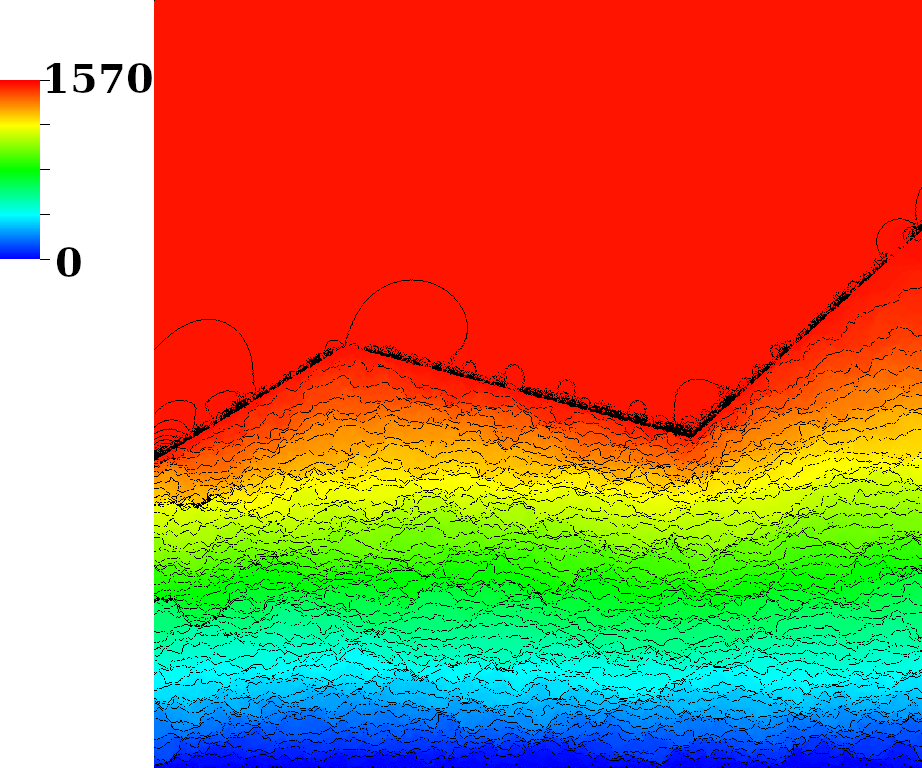
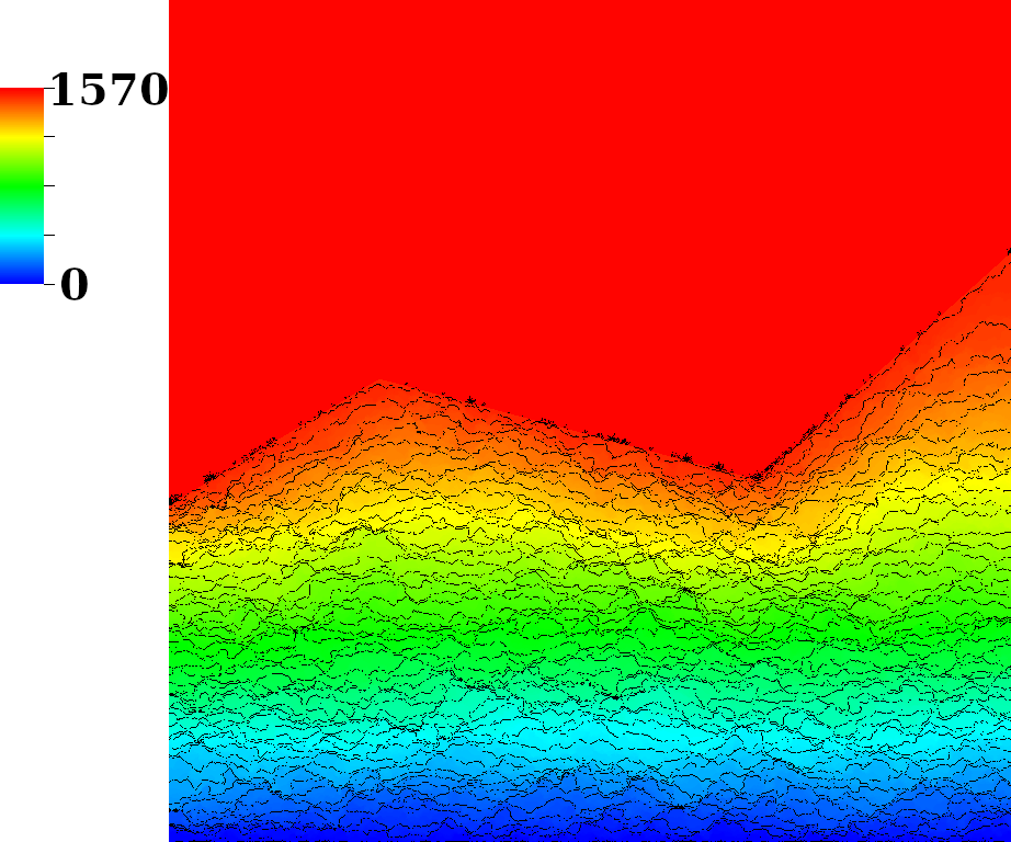
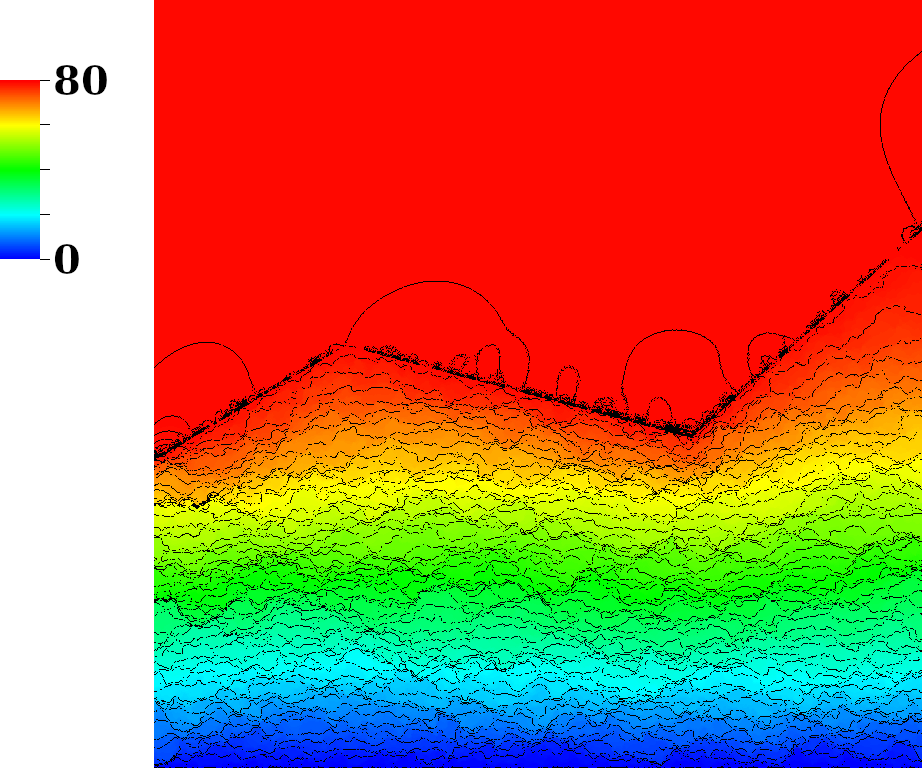
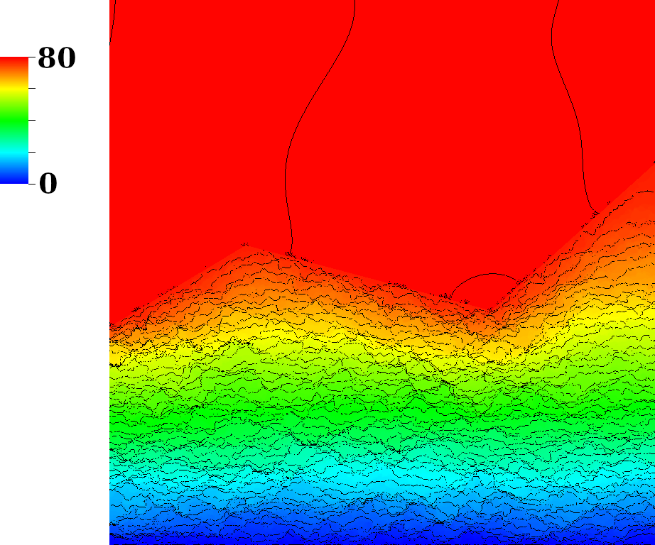
6.2 Surface/subsurface flow with nonuniform permeability field

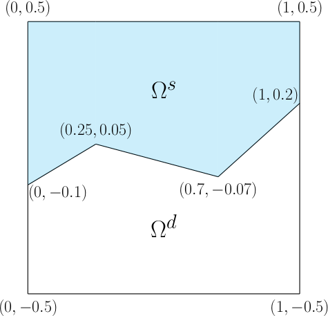
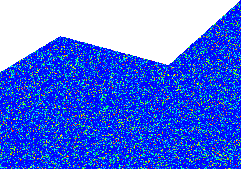
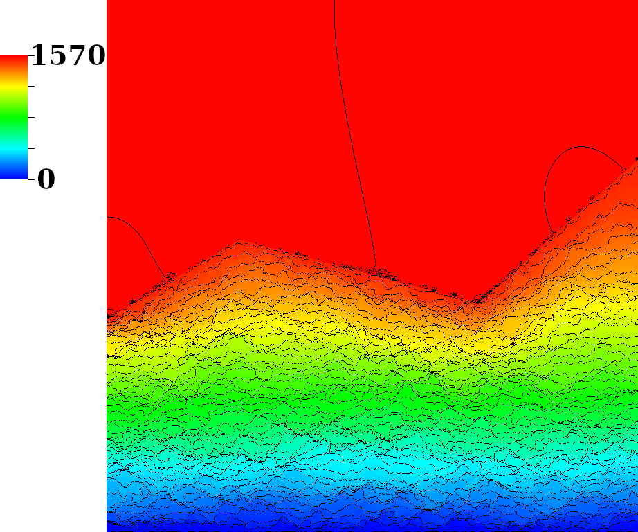
In this example we consider surface/subsurface flow. For this example we divide the domain $\Omega=(0,1)\times(-0.5,0.5)$ into two subdomains $\Omega^{s}$ and $\Omega^{d}$. We consider a case where the interface $\Gamma^{I}=\overline{\Omega^{s}}\cap\overline{\Omega^{d}}$ is not horizontal (see fig. 1a). Furthermore, let $\Gamma_{D}^{d}=\mathinner{\left\{x\in\Gamma^{d}\mathrel{\mathop{\mathchar 58\relax}}\ x_{2}=-0.5\right\}}$, and $\Gamma_{N}^{d}=\Gamma^{d}\backslash\Gamma_{D}^{d}$. We then impose the following boundary conditions:

$$u^{s} =(\tfrac{5}{42}(10x_{2}+1)(1-x_{1}/5)(\cos(\pi t/5)+\tfrac{11}{10}),0) \text{on }\Gamma^{s}\times J,$$

$$u^{d}\cdot n =0 \text{on }\Gamma_{N}^{d}\times J,$$

$$p^{d} =0 \text{on }\Gamma_{D}^{d}\times J,$$

and set $f^{s}=0$ and $f^{d}=0$. We consider both $\mu=10^{-1}$ and $\mu=10^{-3}$ together with $\alpha=0.5$, and choose the permeability to be piecewise constant such that $\mu^{-1}\kappa=10^{-r}$ with $r\in[2,6]$ a random number that is chosen differently in each element of the mesh in $\Omega^{d}$. (The analysis presented in this paper assumes a constant permeability, but noting that $0<\kappa_{\min}\leq\kappa(x)\leq\kappa_{\max}$ the analysis is easily extended to this situation.) A plot of the permeability is given in fig. 1b. To set the initial condition for the velocity in $\Omega^{s}$ we solve the stationary Stokes–Darcy problem.

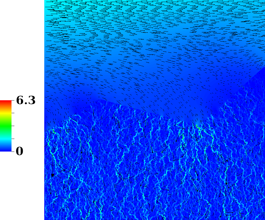
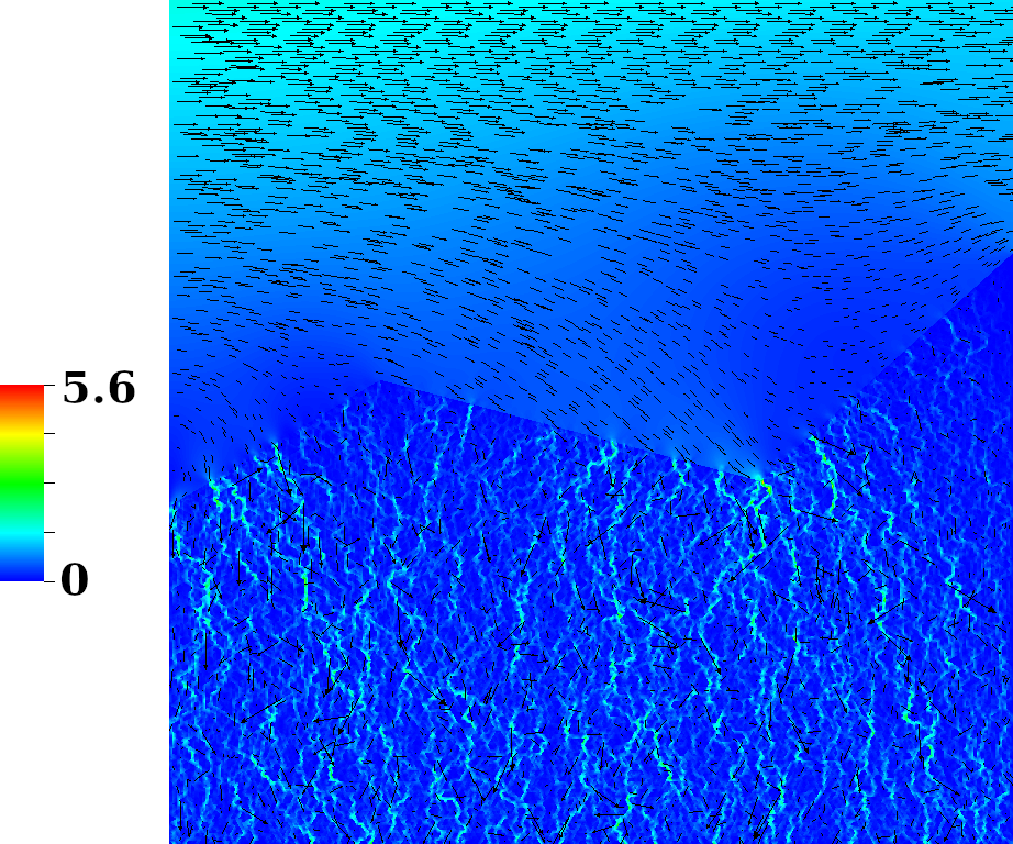
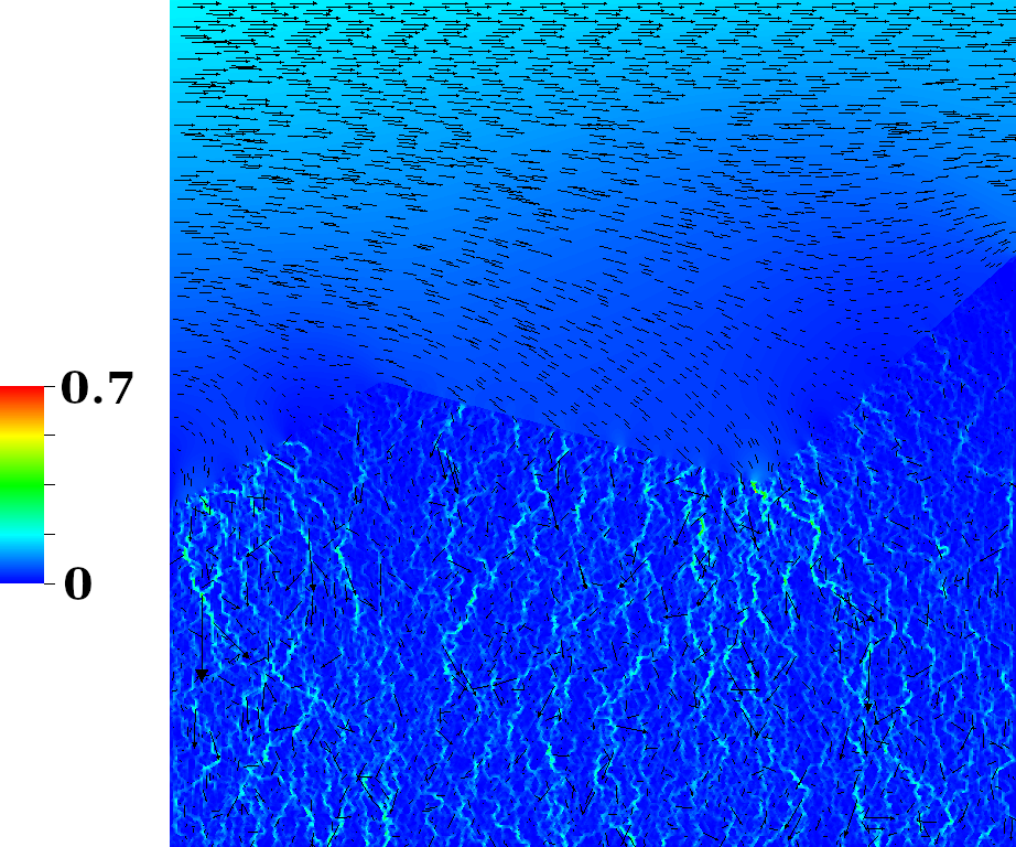
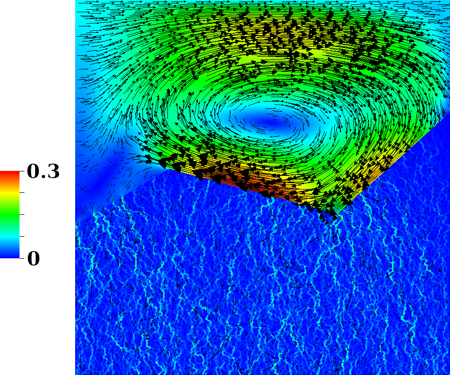
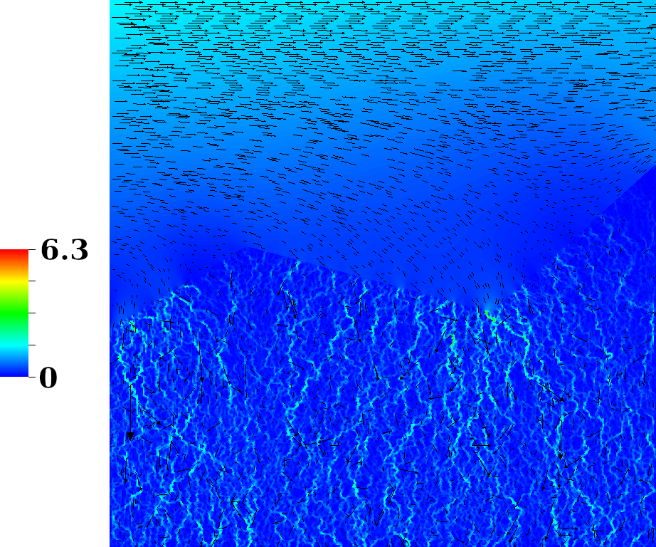
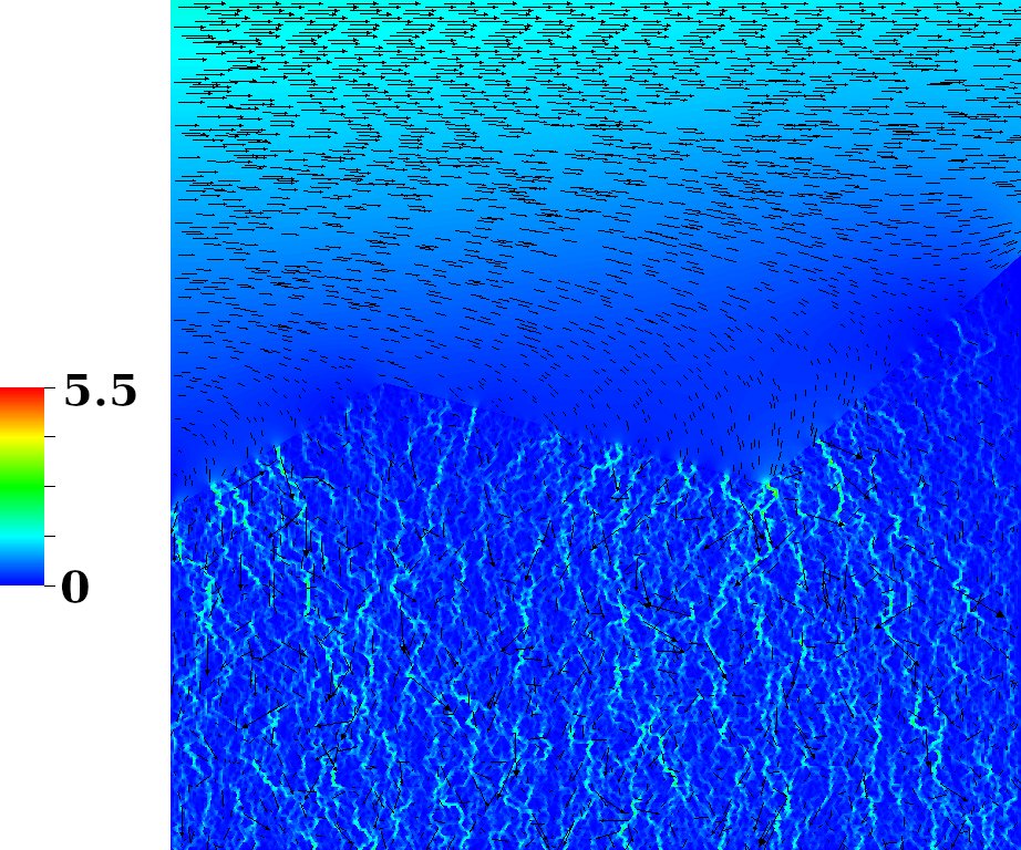
We compute the solution on a mesh consisting of 91720 elements, using $k=2$, a time step of $\Delta t=0.01$, and on the time interval $J=(0,10)$. Plots of the velocity and pressure fields at different time levels are shown in figs. 2 and 3, both for $\mu=10^{-1}$ and $\mu=10^{-3}$. The velocity fields at $t=0$ and $t=10$ for both values of viscosity are similar: flow in $\Omega^{s}$ away from the interface is more or less horizontal while in $\Omega^{d}$ flow finds its way through the permeability maze in the direction of negative pressure gradient. At $t=5.2$ (when the inflow magnitude of the velocity is close to its minimum), the behavior of the velocity fields when $\mu=10^{-1}$ and $\mu=10^{-3}$ are significantly different: when $\mu=10^{-1}$ the velocity field is similar to that at $t=0$ and $t=10$, but when $\mu=10^{-3}$ we obtain a large area of circulation. The pressure fields are similar for the two values of viscosity and follow a more or less linear profile in $\Omega^{d}$. Pressure variations in $\Omega^{s}$ are small.

(a) Domain.

(b) Permeability.

Figure 1: The surface/subsurface domain $\Omega$ used in section 6.2.

(a) $\mu=10^{-1}$, $t=0$.

(b) $\mu=10^{-3}$, $t=0$.

(c) $\mu=10^{-1}$, $t=5.2$.

(d) $\mu=10^{-3}$, $t=5.2$.

(e) $\mu=10^{-1}$, $t=10$.

(f) $\mu=10^{-3}$, $t=10$.

Figure 2: Velocity magnitude and velocity vector field at time levels $t=0$, $t=5.2$, and $t=10$. Left column: $\mu=10^{-1}$. Right column: $\mu=10^{-3}$. See also section 6.2.

(a) $\mu=10^{-1}$, $t=0$.

(b) $\mu=10^{-3}$, $t=0$.

(c) $\mu=10^{-1}$, $t=5.2$.

(d) $\mu=10^{-3}$, $t=5.2$.

(e) $\mu=10^{-1}$, $t=10$.

(f) $\mu=10^{-3}$, $t=10$.

Figure 3: Pressure magnitude and contour plots at time levels $t=0$, $t=5.2$, and $t=10$. Left column: $\mu=10^{-1}$. Right column: $\mu=10^{-3}$. For visualization purposes at $t=0$ and $t=10$ we consider in $\Omega^{d}$ the pressure interval $[0,1570]$ divided into 50 contour lines using a linear scale while in $\Omega^{s}$ we consider the pressure interval $[1500,1570]$ divided into 100 contour lines using a log scale. At $t=5.2$ we consider in $\Omega^{d}$ and $\Omega^{s}$ the pressure intervals $[0,80]$ and $[75,80]$, respectively. See also section 6.2.

7 Conclusions

We presented a strongly conservative HDG method for the coupled time-dependent Navier–Stokes and Darcy problem. Existence and uniqueness of a solution to the fully discrete problem were proven assuming a small data assumption. We furthermore determined a pressure-independent a priori error estimate for the discrete velocity. This estimate is optimal in space in the combined discrete $H^{1}$-norm on $\Omega^{s}$ and $H(\text{div})$-norm on $\Omega^{d}$, and optimal in time. Our analysis is supported by numerical examples.

Acknowledgements

AC and JJL are funded by the National Science Foundation under grant numbers DMS-2110782 and DMS-2110781. SR is funded by the Natural Sciences and Engineering Research Council of Canada through the Discovery Grant program (RGPIN-05606-2015).

Appendix A Proof of the inf-sup condition eq. 9a

An inf-sup condition of the form eq. 9a was proven in [6, Lemma 2] assuming that $u=0$ on $\Gamma^{s}$ and $u\cdot n=0$ on $\Gamma^{d}$. We modify this proof to take into account the boundary conditions eqs. 4b, 4c and 4d. The proof requires the BDM interpolation operator $\Pi_{V}\mathrel{\mathop{\mathchar 58\relax}}H({\rm div};\Omega)\cap\mathinner{[L^{r}(\Omega)]}^{\dim}\rightarrow X_{h}\cap H({\rm div};\Omega)$, $r>2$, which satisfies eqs. 58, 59 and 60 for all $u\in\mathinner{[H^{k+1}(K)]}^{\dim}$. We will also require the following function space:

$$\mathinner{[H^{1}_{0,\Gamma^{s}\cup\Gamma_{N}^{d}}(\Omega)]}^{\dim}\mathrel{\mathop{\mathchar 58\relax}}=\mathinner{\{w\in\mathinner{[H^{1}(\Omega)]}^{\dim}\,\mathrel{\mathop{\mathchar 58\relax}}\,w|_{\Gamma^{s}\cup\Gamma_{N}^{d}}=0\}}.$$

Defining

$$\begin{split}\tilde{b}_{h}(\boldsymbol{v}_{h},(\bar{q}^{s}_{h},\bar{q}^{d}_{h}))&\mathrel{\mathop{\mathchar 58\relax}}=\sum_{j=s,d}\mathinner{\Bigl{(}\langle\bar{q}_{h}^{j},v_{h}\cdot n^{j}\rangle_{\partial\mathcal{T}_{h}^{j}}-\langle\bar{q}_{h}^{j},\bar{v}_{h}\cdot n^{j}\rangle_{\Gamma^{I}}\Bigr{)}},\\ \text{Ker}(\tilde{b}_{h})&\mathrel{\mathop{\mathchar 58\relax}}=\mathinner{\{\boldsymbol{v}_{h}\in\boldsymbol{X}_{h}\,\mathrel{\mathop{\mathchar 58\relax}}\,\tilde{b}_{h}(\boldsymbol{v}_{h},(\bar{q}^{s}_{h},\bar{q}^{d}_{h}))=0\ \forall(\bar{q}_{h}^{s},\bar{q}_{h}^{d})\in\bar{Q}_{h}^{s}\times\bar{Q}_{h}^{d}\}},\end{split}$$

and noting that $b_{h}(\boldsymbol{v}_{h},\boldsymbol{q}_{h})=-(q_{h},\nabla\cdot v_{h})_{\Omega}+\tilde{b}_{h}(\boldsymbol{v}_{h},(\bar{q}^{s}_{h},\bar{q}^{d}_{h}))$, by [24, Theorem 3.1] the inf-sup condition eq. 9a holds for all $\boldsymbol{q}_{h}\in\boldsymbol{Q}_{h}$ if there exist constants $c_{b1}>0$ and $c_{b2}>0$, independent of $h$ and $\Delta t$, such that

$$c_{b1}\mathinner{\lVert q_{h}\rVert}_{\Omega} \leq\sup_{\begin{subarray}{c}\boldsymbol{v}_{h}\in\text{Ker}(\tilde{b}_{h})\\ \boldsymbol{v}_{h}\neq 0\end{subarray}}\frac{-(q_{h},\nabla\cdot v_{h})_{\Omega}}{\mathopen{|\mkern-1.5mu|\mkern-1.5mu|}\boldsymbol{v}_{h}\mathclose{|\mkern-1.5mu|\mkern-1.5mu|}_{v}} \forall q_{h}\in Q_{h},$$ (69a)

$$\mathinner{\Bigl{(}c_{b2}\sum_{j=s,d}\sum_{K\in\mathcal{T}_{h}^{j}}h_{K}\mathinner{\lVert\bar{q}_{h}^{j}\rVert}^{2}_{\partial K}\Bigr{)}}^{1/2} \leq\sup_{\begin{subarray}{c}\boldsymbol{v}_{h}\in\boldsymbol{X}_{h}\\ \boldsymbol{v}_{h}\neq 0\end{subarray}}\frac{\tilde{b}_{h}(\boldsymbol{v}_{h},(\bar{q}^{s}_{h},\bar{q}^{d}_{h}))}{\mathopen{|\mkern-1.5mu|\mkern-1.5mu|}\boldsymbol{v}_{h}\mathclose{|\mkern-1.5mu|\mkern-1.5mu|}_{v}} \forall(\bar{q}_{h}^{s},\bar{q}_{h}^{d})\in\bar{Q}_{h}^{s}\times\bar{Q}_{h}^{d}.$$ (69b)

Compared to [6, Lemma 2], only the proof for eq. 69a needs to be modified.

We first seek a suitable $\boldsymbol{v}_{h}\in\text{Ker}(\tilde{b}_{h})$. Let $q_{h}\in Q_{h}$. By [30, Remark 3.3] there exists $v\in\mathinner{[H^{1}_{0,\Gamma^{s}\cup\Gamma_{N}^{d}}(\Omega)]}^{\dim}$ such that

$$-(\nabla\cdot v,q_{h})_{\Omega}=\mathinner{\lVert q_{h}\rVert}_{\Omega}^{2},\quad c_{vq}\mathinner{\lVert v\rVert}_{1,\Omega}\leq\mathinner{\lVert q_{h}\rVert}_{\Omega},$$ (70)

where $c_{vq}>0$ is a constant independent of $h$ and $\Delta t$. Let $\bar{\Pi}_{V}\mathrel{\mathop{\mathchar 58\relax}}\mathinner{[H^{1}(\Omega^{s})]}^{\dim}\to\bar{X}_{h}$ be the $L^{2}$-projection into the facet velocity space and note that the pair $\boldsymbol{v}_{h}=(\Pi_{V}v,\bar{\Pi}_{V}v)$ lies in $\text{Ker}(\tilde{b}_{h})$:

$$\begin{split}\tilde{b}_{h}((\Pi_{V}v,\bar{\Pi}_{V}v),(\bar{q}^{s}_{h},\bar{q}^{d}_{h}))=&\langle\bar{q}_{h}^{s},(\Pi_{V}v-\bar{\Pi}_{V}v)\cdot n^{s}\rangle_{\Gamma^{I}}+\langle\bar{q}_{h}^{s},\Pi_{V}v\cdot n^{s}\rangle_{\Gamma^{s}}+\langle\bar{q}_{h}^{d},(\Pi_{V}v-\bar{\Pi}_{V}v)\cdot n^{d}\rangle_{\Gamma^{I}}+\langle\bar{q}_{h}^{d},\Pi_{V}v\cdot n^{d}\rangle_{\Gamma^{d}}\\ =&\langle\bar{q}_{h}^{s},(v-v)\cdot n^{s}\rangle_{\Gamma^{I}}+\langle\bar{q}_{h}^{d},(v-v)\cdot n^{d}\rangle_{\Gamma^{I}}=0,\end{split}$$

where the first equality is because $\Pi_{V}v\cdot n^{j}$ is continuous on element boundaries and $\bar{q}_{h}^{j}$ is single-valued. The second equality is by properties of $\Pi_{V}$ and $\bar{\Pi}_{V}$, $v\cdot n^{j}=0$ on $\Gamma^{s}\cup\Gamma_{N}^{d}$, and $\bar{q}_{h}^{d}=0$ on $\Gamma_{D}^{d}$. Therefore, $(\Pi_{V}v,\bar{\Pi}_{V}v)\in\text{Ker}(\tilde{b}_{h})$.

We now proceed to find a bound for $\mathopen{|\mkern-1.5mu|\mkern-1.5mu|}(\Pi_{V}v,\bar{\Pi}_{V}v)\mathclose{|\mkern-1.5mu|\mkern-1.5mu|}_{v}$ in terms of $\mathinner{\!\left\lVert v\right\rVert}_{1,\Omega}$. First, note that by definition,

$$\begin{split}\mathopen{|\mkern-1.5mu|\mkern-1.5mu|}(\Pi_{V}v,\bar{\Pi}_{V}v)\mathclose{|\mkern-1.5mu|\mkern-1.5mu|}_{v,d}^{2}=&\mathinner{\lVert\Pi_{V}v\rVert}_{\text{div};\Omega^{d}}^{2}+\sum_{F\in\mathcal{F}^{d}_{h}\backslash(\mathcal{F}_{h}^{I}\cup\mathcal{F}_{h}^{D,d})}h_{F}^{-1}\mathinner{\lVert\llbracket\Pi_{V}v\cdot n\rrbracket\rVert}_{F}^{2}\\ &+\sum_{K\in\mathcal{T}_{h}^{d}}h_{K}^{-1}\mathinner{\lVert(\Pi_{V}v-\bar{\Pi}_{V}v)\cdot n\rVert}_{\partial K\cap\Gamma^{I}}^{2}=\mathrel{\mathop{\mathchar 58\relax}}I_{1}+I_{2}+I_{3}.\end{split}$$

In [6, Lemma 2] it was shown that $I_{1}+I_{3}\leq C\mathinner{\lVert v\rVert}_{1,\Omega^{d}}^{2}$. Furthermore, $I_{2}=0$ because $\Pi_{V}v\in H(\text{div};\Omega^{d})$ and $v=0$ on $\Gamma_{N}^{d}$. Therefore, $\mathopen{|\mkern-1.5mu|\mkern-1.5mu|}(\Pi_{V}v,\bar{\Pi}_{V}v)\mathclose{|\mkern-1.5mu|\mkern-1.5mu|}_{v,d}\leq C\mathinner{\!\left\lVert v\right\rVert}_{1,\Omega^{d}}$. In the proof of [6, Lemma 2] it was also shown that

$$\mathopen{|\mkern-1.5mu|\mkern-1.5mu|}(\Pi_{V}v,\bar{\Pi}_{V}v)\mathclose{|\mkern-1.5mu|\mkern-1.5mu|}_{v,s}\leq C\mathinner{\lVert v\rVert}_{1,\Omega^{s}},\quad\mathinner{\lVert(\bar{\Pi}_{V}v)^{t}\rVert}_{\Gamma^{I}}\leq C\mathinner{\lVert v\rVert}_{1,\Omega^{s}}.$$ (71)

By definition of $\mathopen{|\mkern-1.5mu|\mkern-1.5mu|}\cdot\mathclose{|\mkern-1.5mu|\mkern-1.5mu|}_{v}$ and using the preceding bounds on $\mathopen{|\mkern-1.5mu|\mkern-1.5mu|}(\Pi_{V}v,\bar{\Pi}_{V}v)\mathclose{|\mkern-1.5mu|\mkern-1.5mu|}_{v,s}$, $\mathinner{\lVert(\bar{\Pi}_{V}v)^{t}\rVert}_{\Gamma^{I}}$, and $\mathopen{|\mkern-1.5mu|\mkern-1.5mu|}(\Pi_{V}v,\bar{\Pi}_{V}v)\mathclose{|\mkern-1.5mu|\mkern-1.5mu|}_{v,d}$, we find

$$\mathopen{|\mkern-1.5mu|\mkern-1.5mu|}(\Pi_{V}v,\bar{\Pi}_{V}v)\mathclose{|\mkern-1.5mu|\mkern-1.5mu|}_{v}\leq C\mathinner{\!\left\lVert v\right\rVert}_{1,\Omega}.$$

Equation 69a now follows from this and eq. 70:

$$\sup_{\begin{subarray}{c}\boldsymbol{v}_{h}\in\text{Ker}(\tilde{b}_{h})\\ \boldsymbol{v}_{h}\neq 0\end{subarray}}\frac{-(q_{h},\nabla\cdot v_{h})_{\Omega}}{\mathopen{|\mkern-1.5mu|\mkern-1.5mu|}\boldsymbol{v}_{h}\mathclose{|\mkern-1.5mu|\mkern-1.5mu|}_{v}}\geq\frac{-(q_{h},\nabla\cdot\Pi_{V}v)_{\Omega}}{\mathopen{|\mkern-1.5mu|\mkern-1.5mu|}(\Pi_{V}v,\bar{\Pi}_{V}v)\mathclose{|\mkern-1.5mu|\mkern-1.5mu|}_{v}}\geq\frac{\mathinner{\lVert q_{h}\rVert}^{2}_{\Omega}}{C\mathinner{\lVert v\rVert}_{1,\Omega}}\geq\frac{c_{vq}}{C}\mathinner{\lVert q_{h}\rVert}_{\Omega}.$$

Appendix B Useful inequalities

Let $g$ be a sufficiently smooth function. Using Taylor’s theorem in integral form, it is shown in [26, Lemma 7.67]) that

$$\mathinner{\lVert\partial_{t}g^{n+1}-d_{t}g^{n+1}\rVert}_{\Omega^{s}}\leq C\sqrt{\Delta t}\mathinner{\lVert\partial_{tt}g\rVert}_{L^{2}(t^{n},t^{n+1};L^{2}(\Omega^{s}))}.$$ (72)

A minor modification of the proof of eq. 72 leads to:

$$\mathinner{\lVert g^{n+1}-g^{n}\rVert}_{\Omega^{s}}\leq C\Delta t(\mathinner{\lVert\partial_{t}g^{n}\rVert}_{\Omega^{s}}+\mathinner{\lVert\partial_{tt}g\rVert}_{L^{2}(t^{n},t^{n+1};L^{2}(\Omega^{s}))}).$$ (73)

We also have, by the fundamental theorem of Calculus and the Cauchy–Schwarz inequality, that

$$\mathinner{\lVert g^{n+1}-g^{n}\rVert}_{\Omega^{s}}=\mathinner{\lVert\int_{t^{n}}^{t^{n+1}}\partial_{t}g\operatorname{d\!}t\rVert}\leq\mathinner{\Bigl{(}\int_{t^{n}}^{t^{n+1}}\operatorname{d\!}t\Bigr{)}}^{1/2}\mathinner{\Bigl{(}\int_{t^{n}}^{t^{n+1}}\mathinner{\lVert\partial_{t}g\rVert}_{\Omega^{s}}^{2}\operatorname{d\!}t\Bigr{)}}^{1/2}\leq\sqrt{\Delta t}\mathinner{\lVert\partial_{t}g\rVert}_{L^{2}(t^{n},t^{n+1};L^{2}(\Omega^{s}))}.$$ (74)

Appendix C Proof of eq. 68

To prove eq. 68 we will use the following result, which is due to a discrete Sobolev embedding [17, Theorem 5.3] and eq. 8b:

$$\mathinner{\Bigl{(}\sum_{K\in\mathcal{T}_{h}^{s}}\mathinner{\lVert v_{h}\rVert}_{L^{6}(K)}^{6}\Bigr{)}}^{1/6}\leq C\mathopen{|\mkern-1.5mu|\mkern-1.5mu|}\boldsymbol{v}_{h}\mathclose{|\mkern-1.5mu|\mkern-1.5mu|}_{v,s}\quad\forall\boldsymbol{v}_{h}\in\boldsymbol{X}_{h}.$$ (75)

Let us first write $I_{4}$ as:

$$\begin{split}I_{4}=&[t_{h}(u^{n};\boldsymbol{\Pi}_{V}u^{n+1},\boldsymbol{e}_{u}^{h,n+1})-t_{h}(u_{h}^{n};\boldsymbol{\Pi}_{V}u^{n+1},\boldsymbol{e}_{u}^{h,n+1})]\\ =&[t_{h}(u^{n};\boldsymbol{u}^{n+1},\boldsymbol{e}_{u}^{h,n+1})-t_{h}(u^{n};\boldsymbol{u}^{n+1}-\boldsymbol{\Pi}_{V}u^{n+1},\boldsymbol{e}_{u}^{h,n+1})]\\ &-[t_{h}(u_{h}^{n};\boldsymbol{u}^{n+1},\boldsymbol{e}_{u}^{h,n+1})-t_{h}(u_{h}^{n};\boldsymbol{u}^{n+1}-\boldsymbol{\Pi}_{V}u^{n+1},\boldsymbol{e}_{u}^{h,n+1})]\\ =&[t_{h}(u^{n};\boldsymbol{u}^{n+1},\boldsymbol{e}_{u}^{h,n+1})-t_{h}(u_{h}^{n};\boldsymbol{u}^{n+1},\boldsymbol{e}_{u}^{h,n+1})]\\ &+[t_{h}(u_{h}^{n};\boldsymbol{u}^{n+1}-\boldsymbol{\Pi}_{V}u^{n+1},\boldsymbol{e}_{u}^{h,n+1})-t_{h}(u^{n};\boldsymbol{u}^{n+1}-\boldsymbol{\Pi}_{V}u^{n+1},\boldsymbol{e}_{u}^{h,n+1})]\\ =&\mathrel{\mathop{\mathchar 58\relax}}I_{41}+I_{42}.\end{split}$$

For $I_{41}$ we note that since the second argument of $t_{h}$ is continuous almost everywhere:

$$I_{41}=t_{h}(u^{n}-u_{h}^{n};\boldsymbol{u}^{n+1},\boldsymbol{e}_{u}^{h,n+1})=t_{h}(e_{u}^{I,n};\boldsymbol{u}^{n+1},\boldsymbol{e}_{u}^{h,n+1})-t_{h}(e_{u}^{h,n};\boldsymbol{u}^{n+1},\boldsymbol{e}_{u}^{h,n+1})=\mathrel{\mathop{\mathchar 58\relax}}I_{411}+I_{412}.$$

We have by eq. 13 and Young’s inequality,

$$\begin{split}I_{411}&\leq c_{w}\mathinner{\lVert e_{u}^{I,n}\rVert}_{1,h,\Omega^{s}}\mathopen{|\mkern-1.5mu|\mkern-1.5mu|}\boldsymbol{u}^{n+1}\mathclose{|\mkern-1.5mu|\mkern-1.5mu|}_{v,s}\mathopen{|\mkern-1.5mu|\mkern-1.5mu|}\boldsymbol{e}_{u}^{h,n+1}\mathclose{|\mkern-1.5mu|\mkern-1.5mu|}_{v,s}\\ &\leq Ch^{k}\mathinner{\lVert u^{n}\rVert}_{k+1,\Omega^{s}}\mathinner{\lVert\nabla u^{n+1}\rVert}_{\Omega^{s}}\mathopen{|\mkern-1.5mu|\mkern-1.5mu|}\boldsymbol{e}_{u}^{h,n+1}\mathclose{|\mkern-1.5mu|\mkern-1.5mu|}_{v,s}\\ &\leq\tfrac{1}{2}\gamma\mathopen{|\mkern-1.5mu|\mkern-1.5mu|}\boldsymbol{e}_{u}^{h,n+1}\mathclose{|\mkern-1.5mu|\mkern-1.5mu|}_{v,s}^{2}+\frac{C}{\gamma}h^{2k}\mathinner{\lVert u^{n}\rVert}_{k+1,\Omega^{s}}^{2}\mathinner{\lVert\nabla u^{n+1}\rVert}_{\Omega^{s}}^{2}.\end{split}$$ (76)

Next, using that $u^{n+1}=\bar{u}^{n+1}$ on facets,

$$I_{412}=-(u^{n+1}\otimes e_{u}^{h,n},\nabla e_{u}^{h,n+1})_{\Omega^{s}}+\langle e_{u}^{h,n}\cdot n,(e_{u}^{h,n+1}-\bar{e}_{u}^{h,n+1})\cdot u^{n+1}\rangle_{\partial\mathcal{T}_{h}^{s}}+\langle e_{u}^{h,n}\cdot n,\bar{e}_{u}^{h,n+1}\cdot u^{n+1}\rangle_{\Gamma^{I}}.$$

At this point we note that since $e_{u}^{h,n}\cdot n$, $\bar{e}_{u}^{h,n+1}$, and $u^{n+1}$ are single-valued on facets, and because $u=0$ on $\Gamma^{s}$, we have that $\langle e_{u}^{h,n}\cdot n,\bar{e}_{u}^{h,n+1}\cdot u^{n+1}\rangle_{\partial\mathcal{T}_{h}^{s}}=\langle e_{u}^{h,n}\cdot n,\bar{e}_{u}^{h,n+1}\cdot u^{n+1}\rangle_{\Gamma^{I}}$. Therefore,

$$I_{412}=-(u^{n+1}\otimes e_{u}^{h,n},\nabla e_{u}^{h,n+1})_{\Omega^{s}}+\langle e_{u}^{h,n}\cdot n,e_{u}^{h,n+1}\cdot u^{n+1}\rangle_{\partial\mathcal{T}_{h}^{s}}.$$

Integrating by parts, using that $\nabla\cdot e_{u}^{h,n}=0$ on each $K\in\mathcal{T}^{s}_{h}$, the generalized Hölder’s inequality, eq. 75, and Young’s inequality:

$$\begin{split}I_{412}=&(\nabla\cdot(u^{n+1}\otimes e_{u}^{h,n}),e_{u}^{h,n+1})_{\Omega^{s}}=(e_{u}^{h,n}\cdot\nabla u^{n+1},e_{u}^{h,n+1})_{\Omega^{s}}\\ \leq&\mathinner{\lVert e_{u}^{h,n}\rVert}_{\Omega^{s}}|u^{n+1}|_{W^{1}_{3}(\Omega^{s})}\mathinner{\lVert e_{u}^{h,n+1}\rVert}_{L^{6}(\Omega^{s})}\\ \leq&C\mathinner{\lVert e_{u}^{h,n}\rVert}_{\Omega^{s}}|u^{n+1}|_{W^{1}_{3}(\Omega^{s})}\mathopen{|\mkern-1.5mu|\mkern-1.5mu|}\boldsymbol{e}_{u}^{h,n+1}\mathclose{|\mkern-1.5mu|\mkern-1.5mu|}_{v,s}\\ \leq&\tfrac{1}{2}\gamma\mathopen{|\mkern-1.5mu|\mkern-1.5mu|}\boldsymbol{e}_{u}^{h,n+1}\mathclose{|\mkern-1.5mu|\mkern-1.5mu|}_{v}^{2}+\frac{C}{\gamma}\mathinner{\lVert e_{u}^{h,n}\rVert}_{\Omega^{s}}^{2}|u^{n+1}|_{W^{1}_{3}(\Omega^{s})}^{2}.\end{split}$$ (77)

Combining eqs. 76 and 77 we find

$$I_{41}\leq\gamma\mathopen{|\mkern-1.5mu|\mkern-1.5mu|}\boldsymbol{e}_{u}^{h,n+1}\mathclose{|\mkern-1.5mu|\mkern-1.5mu|}_{v}^{2}+\frac{C}{\gamma}h^{2k}\mathinner{\lVert u^{n}\rVert}_{k+1,\Omega^{s}}^{2}\mathinner{\lVert\nabla u^{n+1}\rVert}_{\Omega^{s}}^{2}+\frac{C}{\gamma}\mathinner{\lVert e_{u}^{h,n}\rVert}_{\Omega^{s}}^{2}|u^{n+1}|_{W^{1}_{3}(\Omega^{s})}^{2}.$$ (78)

We next consider $I_{42}$ which we first write as:

$$\begin{split}I_{42}=&[t_{h}(u_{h}^{n};\boldsymbol{u}^{n+1}-\boldsymbol{\Pi}_{V}u^{n+1},\boldsymbol{e}_{u}^{h,n+1})-t_{h}(\Pi_{V}u^{n};\boldsymbol{u}^{n+1}-\boldsymbol{\Pi}_{V}u^{n+1},\boldsymbol{e}_{u}^{h,n+1})]\\ &+[t_{h}(\Pi_{V}u^{n};\boldsymbol{u}^{n+1}-\boldsymbol{\Pi}_{V}u^{n+1},\boldsymbol{e}_{u}^{h,n+1})-t_{h}(u^{n};\boldsymbol{u}^{n+1}-\boldsymbol{\Pi}_{V}u^{n+1},\boldsymbol{e}_{u}^{h,n+1})]\\ =&[t_{h}(\Pi_{V}u^{n};\boldsymbol{e}_{u}^{I,n+1},\boldsymbol{e}_{u}^{h,n+1})-t_{h}(u^{n};\boldsymbol{e}_{u}^{I,n+1},\boldsymbol{e}_{u}^{h,n+1})]\\ &+[t_{h}(u_{h}^{n};\boldsymbol{e}_{u}^{I,n+1},\boldsymbol{e}_{u}^{h,n+1})-t_{h}(\Pi_{V}u^{n};\boldsymbol{e}_{u}^{I,n+1},\boldsymbol{e}_{u}^{h,n+1})]\\ =&\mathrel{\mathop{\mathchar 58\relax}}I_{421}+I_{422}.\end{split}$$

For $I_{421}$ we have by eq. 13, [6, Lemma 7], properties of $\Pi_{V}$ and $\bar{\Pi}_{V}$, and Young’s inequality,

$$\begin{split}I_{421}&\leq c_{w}\mathinner{\!\left\lVert\Pi_{V}u^{n}-u^{n}\right\rVert}_{1,h,\Omega^{s}}\mathopen{|\mkern-1.5mu|\mkern-1.5mu|}\boldsymbol{e}_{u}^{I,n+1}\mathclose{|\mkern-1.5mu|\mkern-1.5mu|}_{v,s}\mathopen{|\mkern-1.5mu|\mkern-1.5mu|}\boldsymbol{e}_{u}^{h,n+1}\mathclose{|\mkern-1.5mu|\mkern-1.5mu|}_{v,s}\\ &=c_{w}\mathinner{\lVert e_{u}^{I,n}\rVert}_{1,h,\Omega^{s}}\mathopen{|\mkern-1.5mu|\mkern-1.5mu|}\boldsymbol{e}_{u}^{I,n+1}\mathclose{|\mkern-1.5mu|\mkern-1.5mu|}_{v,s}\mathopen{|\mkern-1.5mu|\mkern-1.5mu|}\boldsymbol{e}_{u}^{h,n+1}\mathclose{|\mkern-1.5mu|\mkern-1.5mu|}_{v,s}\\ &\leq Ch^{k}\mathinner{\lVert u^{n+1}\rVert}_{k+1,\Omega^{s}}\mathinner{\lVert e_{u}^{I,n}\rVert}_{1,h,\Omega^{s}}\mathopen{|\mkern-1.5mu|\mkern-1.5mu|}\boldsymbol{e}_{u}^{h,n+1}\mathclose{|\mkern-1.5mu|\mkern-1.5mu|}_{v,s}\\ &\leq Ch^{2k}\mathinner{\lVert u^{n+1}\rVert}_{k+1,\Omega^{s}}\mathinner{\lVert u^{n}\rVert}_{k+1,\Omega^{s}}\mathopen{|\mkern-1.5mu|\mkern-1.5mu|}\boldsymbol{e}_{u}^{h,n+1}\mathclose{|\mkern-1.5mu|\mkern-1.5mu|}_{v,s}\\ &\leq\tfrac{1}{2}\gamma\mathopen{|\mkern-1.5mu|\mkern-1.5mu|}\boldsymbol{e}_{u}^{h,n+1}\mathclose{|\mkern-1.5mu|\mkern-1.5mu|}_{v}^{2}+\frac{C}{\gamma}h^{4k}\mathinner{\lVert u^{n+1}\rVert}_{k+1,\Omega^{s}}^{2}\mathinner{\lVert u^{n}\rVert}_{k+1,\Omega^{s}}^{2}.\end{split}$$ (79)

For $I_{422}$ we find, after integrating by parts,

$$\begin{split}I_{422}=&t_{h}(u_{h}^{n};\boldsymbol{e}_{u}^{I,n+1},\boldsymbol{e}_{u}^{h,n+1})-t_{h}(\Pi_{V}u^{n};\boldsymbol{e}_{u}^{I,n+1},\boldsymbol{e}_{u}^{h,n+1})\\ =&(\nabla e_{u}^{I,n+1},e_{u}^{h,n+1}\otimes(u_{h}^{n}-\Pi_{V}u^{n}))_{\Omega^{s}}-\langle((e_{u}^{I,n+1}-\bar{e}_{u}^{I,n+1})\otimes(u_{h}^{n}-\Pi_{V}u^{n}))n,e_{u}^{h,n+1}\rangle_{\partial\mathcal{T}^{s}}\\ &+\langle(\max(u_{h}^{n}\cdot n,0)-\max(\Pi_{V}u^{n}\cdot n,0))(e_{u}^{I,n+1}-\bar{e}_{u}^{I,n+1}),e_{u}^{h,n+1}-\bar{e}_{u}^{h,n+1}\rangle_{\partial\mathcal{T}^{s}}\\ =&(\nabla e_{u}^{I,n+1},e_{u}^{h,n+1}\otimes e_{u}^{h,n})_{\Omega^{s}}-\langle((e_{u}^{I,n+1}-\bar{e}_{u}^{I,n+1})\otimes e_{u}^{h,n})n,e_{u}^{h,n+1}\rangle_{\partial\mathcal{T}^{s}}\\ &+\langle(\max(u_{h}^{n}\cdot n,0)-\max(\Pi_{V}u^{n}\cdot n,0))(e_{u}^{I,n+1}-\bar{e}_{u}^{I,n+1}),e_{u}^{h,n+1}-\bar{e}_{u}^{h,n+1}\rangle_{\partial\mathcal{T}^{s}}\\ =&(e_{u}^{h,n}\cdot\nabla e_{u}^{I,n+1},e_{u}^{h,n+1})_{\Omega^{s}}-\langle e_{u}^{h,n}\cdot n,e_{u}^{h,n+1}\cdot(e_{u}^{I,n+1}-\bar{e}_{u}^{I,n+1})\rangle_{\partial\mathcal{T}^{s}}\\ &+\langle(\max(u_{h}^{n}\cdot n,0)-\max(\Pi_{V}u^{n}\cdot n,0))(e_{u}^{I,n+1}-\bar{e}_{u}^{I,n+1}),e_{u}^{h,n+1}-\bar{e}_{u}^{h,n+1}\rangle_{\partial\mathcal{T}^{s}}\\ =&I_{422a}+I_{422b}+I_{422c}.\end{split}$$

For $I_{422a}$, using generalized Hölder’s inequality, eq. 75, that $|u^{n+1}-\Pi_{V}u^{n+1}|_{W_{3}^{1}(\Omega^{s})}\leq c|u^{n+1}|_{W_{3}^{1}(\Omega^{s})}$ (see [20, Theorem 16.4]) we have:

$$\begin{split}I_{422a}&=(e_{u}^{h,n}\cdot\nabla e_{u}^{I,n+1},e_{u}^{h,n+1})_{\Omega^{s}}\\ &\leq\mathinner{\lVert e_{u}^{h,n}\rVert}_{\Omega^{s}}\mathinner{\lVert\nabla e_{u}^{I,n+1}\rVert}_{L^{3}(\Omega^{s})}\mathinner{\lVert e_{u}^{h,n+1}\rVert}_{L^{6}(\Omega^{s})}\\ &\leq C\mathinner{\lVert e_{u}^{h,n}\rVert}_{\Omega^{s}}|e_{u}^{I,n+1}|_{W_{3}^{1}(\Omega^{s})}\mathopen{|\mkern-1.5mu|\mkern-1.5mu|}\boldsymbol{e}_{u}^{h,n+1}\mathclose{|\mkern-1.5mu|\mkern-1.5mu|}_{v,s}\\ &=C\mathinner{\lVert e_{u}^{h,n}\rVert}_{\Omega^{s}}|u^{n+1}-\Pi_{V}u^{n+1}|_{W_{3}^{1}(\Omega^{s})}\mathopen{|\mkern-1.5mu|\mkern-1.5mu|}\boldsymbol{e}_{u}^{h,n+1}\mathclose{|\mkern-1.5mu|\mkern-1.5mu|}_{v,s}\\ &\leq C\mathinner{\lVert e_{u}^{h,n}\rVert}_{\Omega^{s}}|u^{n+1}|_{W_{3}^{1}(\Omega^{s})}\mathopen{|\mkern-1.5mu|\mkern-1.5mu|}\boldsymbol{e}_{u}^{h,n+1}\mathclose{|\mkern-1.5mu|\mkern-1.5mu|}_{v,s}.\end{split}$$ (80)

To bound $I_{422b}$ let us first consider a single facet $F\subset\partial K$. By Hölder’s inequality,

$$|\langle e_{u}^{h,n}\cdot n,e_{u}^{h,n+1}\cdot(e_{u}^{I,n+1}-\bar{e}_{u}^{I,n+1})\rangle_{F}|\leq\mathinner{\lVert e_{u}^{h,n}\rVert}_{L^{3/2}(F)}\mathinner{\lVert e_{u}^{I,n+1}-\bar{e}_{u}^{I,n+1}\rVert}_{L^{3}(F)}\mathinner{\lVert e_{u}^{h,n+1}\rVert}_{L^{\infty}(F)}.$$ (81)

Noting that $\bar{\Pi}_{V}\Pi_{V}u=\Pi_{V}u$ on $F$, we have:

$$\begin{split}\mathinner{\lVert e_{u}^{I,n+1}-\bar{e}_{u}^{I,n+1}\rVert}_{L^{3}(F)}&=\mathinner{\lVert u^{n+1}-\Pi_{V}u^{n+1}-\gamma(u^{n+1})+\bar{\Pi}_{V}u^{n+1}\rVert}_{L^{3}(F)}\\ &=\mathinner{\lVert\bar{\Pi}_{V}u^{n+1}-\Pi_{V}u^{n+1}\rVert}_{L^{3}(F)}\\ &=\mathinner{\lVert\bar{\Pi}_{V}(u^{n+1}-\Pi_{V}u^{n+1})\rVert}_{L^{3}(F)}\\ &\leq C\mathinner{\lVert u^{n+1}-\Pi_{V}u^{n+1}\rVert}_{L^{3}(F)},\end{split}$$ (82)

where the inequality is by [20, Lemma 11.18]. By a multiplicative trace inequality [20, Lemma 12.15], we have that

$$\mathinner{\lVert u^{n+1}-\Pi_{V}u^{n+1}\rVert}_{L^{3}(F)}\\ \leq c\mathinner{\lVert u^{n+1}-\Pi_{V}u^{n+1}\rVert}_{L^{3}(K)}^{2/3}\mathinner{\bigl{(}h_{K}^{-1/3}\mathinner{\lVert u^{n+1}-\Pi_{V}u^{n+1}\rVert}_{L^{3}(K)}^{1/3}+\mathinner{\lVert\nabla(u^{n+1}-\Pi_{V}u^{n+1})\rVert}_{L^{3}(K)}^{1/3}\bigr{)}},$$ (83)

and by [20, Theorem 16.4] we have

$$\begin{split}\mathinner{\lVert u^{n+1}-\Pi_{V}u^{n+1}\rVert}_{L^{3}(K)}\leq&ch_{K}|\nabla u^{n+1}|_{W^{1}_{3}(K)},\\ \mathinner{\lVert\nabla(u^{n+1}-\Pi_{V}u^{n+1})\rVert}_{L^{3}(K)}\leq&c\mathinner{\lVert u^{n+1}\rVert}_{W^{1}_{3}(K)}.\end{split}$$ (84)

Combining eqs. 82, 83 and 84,

$$\begin{split}\mathinner{\lVert e_{u}^{I,n+1}-\bar{e}_{u}^{I,n+1}\rVert}_{L^{3}(F)}&\leq ch_{K}^{2/3}|\nabla u^{n+1}|_{W^{1}_{3}(K)}^{2/3}\mathinner{\bigl{(}h_{K}^{-1/3}h_{K}^{1/3}|\nabla u^{n+1}|_{W^{1}_{3}(K)}^{1/3}+\mathinner{\lVert u^{n+1}\rVert}_{W^{1}_{3}(K)}^{1/3}\bigr{)}}\\ &\leq ch_{K}^{2/3}\mathinner{\lVert u^{n+1}\rVert}_{W_{3}^{1}(K)}.\end{split}$$ (85)

We also have, by a discrete trace inequality [17, Lemma 1.52], that

$$\mathinner{\lVert e_{u}^{h,n}\rVert}_{L^{3/2}(F)}\leq Ch_{K}^{-2/3}\mathinner{\lVert e_{u}^{h,n}\rVert}_{L^{3/2}(K)},\qquad\mathinner{\lVert e_{u}^{h,n+1}\rVert}_{L^{\infty}(F)}\leq C\mathinner{\lVert e_{u}^{h,n+1}\rVert}_{L^{\infty}(K)}.$$ (86)

Combining eq. 81 with eqs. 85 and 86

$$\begin{split}|\langle e_{u}^{h,n}\cdot n,e_{u}^{h,n+1}\cdot(e_{u}^{I,n+1}-\bar{e}_{u}^{I,n+1})\rangle_{F}|\leq&Ch_{K}^{-2/3}\mathinner{\lVert e_{u}^{h,n}\rVert}_{L^{3/2}(K)}h_{K}^{2/3}\mathinner{\lVert u^{n+1}\rVert}_{W_{3}^{1}(K)}\mathinner{\lVert e_{u}^{h,n+1}\rVert}_{L^{\infty}(K)}\\ =&C\mathinner{\lVert e_{u}^{h,n}\rVert}_{L^{3/2}(K)}\mathinner{\lVert u^{n+1}\rVert}_{W_{3}^{1}(K)}\mathinner{\lVert e_{u}^{h,n+1}\rVert}_{L^{\infty}(K)}.\end{split}$$

By [17, Lemma 1.50], for $\dim=2,3$,

$$\mathinner{\lVert e_{u}^{h,n}\rVert}_{L^{3/2}(K)} \leq Ch_{K}^{\dim/6}\mathinner{\lVert e_{u}^{h,n}\rVert}_{L^{2}(K)},$$ (87a)

$$\mathinner{\lVert e_{u}^{h,n+1}\rVert}_{L^{\infty}(K)} \leq Ch_{K}^{-\dim/6}\mathinner{\lVert e_{u}^{h,n+1}\rVert}_{L^{6}(K)},$$ (87b)

so that

$$|\langle e_{u}^{h,n}\cdot n,e_{u}^{h,n+1}\cdot(e_{u}^{I,n+1}-\bar{e}_{u}^{I,n+1})\rangle_{F}|\leq C\mathinner{\lVert e_{u}^{h,n}\rVert}_{L^{2}(K)}\mathinner{\lVert u^{n+1}\rVert}_{W_{3}^{1}(K)}\mathinner{\lVert e_{u}^{h,n+1}\rVert}_{L^{6}(K)}.$$

Since we assumed $F\subset\partial K$ it follows that

$$|\langle e_{u}^{h,n}\cdot n,e_{u}^{h,n+1}\cdot(e_{u}^{I,n+1}-\bar{e}_{u}^{I,n+1})\rangle_{\partial K}|\leq C\mathinner{\lVert e_{u}^{h,n}\rVert}_{L^{2}(K)}\mathinner{\lVert u^{n+1}\rVert}_{W_{3}^{1}(K)}\mathinner{\lVert e_{u}^{h,n+1}\rVert}_{L^{6}(K)}.$$

Summing over all elements in $\mathcal{T}_{h}^{s}$, using a generalized Hölder’s inequality for the summation over the elements, and eq. 75,

$$\begin{split}I_{422b}&\leq C\sum_{K\in\mathcal{T}_{h}^{s}}\mathinner{\lVert e_{u}^{h,n}\rVert}_{L^{2}(K)}\mathinner{\lVert u^{n+1}\rVert}_{W_{3}^{1}(K)}\mathinner{\lVert e_{u}^{h,n+1}\rVert}_{L^{6}(K)}\\ &\leq C\mathinner{\Bigl{(}\sum_{K\in\mathcal{T}_{h}^{s}}\mathinner{\lVert e_{u}^{h,n}\rVert}_{L^{2}(K)}^{2}\Bigr{)}}^{1/2}\mathinner{\Bigl{(}\sum_{K\in\mathcal{T}_{h}^{s}}\mathinner{\lVert u^{n+1}\rVert}_{W_{3}^{1}(K)}^{3}\Bigr{)}}^{1/3}\mathinner{\Bigl{(}\sum_{K\in\mathcal{T}_{h}^{s}}\mathinner{\lVert e_{u}^{h,n+1}\rVert}_{L^{6}(K)}^{6}\Bigr{)}}^{1/6}\\ &\leq C\mathinner{\lVert e_{u}^{h,n}\rVert}_{L^{2}(\Omega^{s})}\mathinner{\lVert u^{n+1}\rVert}_{W_{3}^{1}(\Omega^{s})}\mathopen{|\mkern-1.5mu|\mkern-1.5mu|}\boldsymbol{e}_{u}^{h,n+1}\mathclose{|\mkern-1.5mu|\mkern-1.5mu|}_{v,s}.\end{split}$$ (88)

Let us now consider $I_{422c}$. Starting again with a single facet $F\subset\partial K$, we find using Hölder’s inequality,

$$\begin{split}&|\langle(\max(u_{h}^{n}\cdot n,0)-\max(\Pi_{V}u^{n}\cdot n,0))(e_{u}^{I,n+1}-\bar{e}_{u}^{I,n+1}),e_{u}^{h,n+1}-\bar{e}_{u}^{h,n+1}\rangle_{F}|\\ &\leq\mathinner{\lVert(\max(u_{h}^{n}\cdot n,0)-\max(\Pi_{V}u^{n}\cdot n,0))\rVert}_{L^{3/2}(F)}\mathinner{\lVert e_{u}^{I,n+1}-\bar{e}_{u}^{I,n+1}\rVert}_{L^{3}(F)}\times\\ &\hskip 200.0003pt\mathinner{\lVert e_{u}^{h,n+1}-\bar{e}_{u}^{h,n+1}\rVert}_{L^{\infty}(F)}.\end{split}$$ (89)

Since $a\mapsto\max(a,0)$ is Lipschitz ([10, Appendix A.3.1]), and using eq. 86:

$$\mathinner{\lVert\max(u_{h}^{n}\cdot n,0)-\max(\Pi_{V}u^{n}\cdot n,0)\rVert}_{L^{3/2}(F)}\\ \leq C\mathinner{\lVert u_{h}^{n}-\Pi_{V}u^{n}\rVert}_{L^{3/2}(F)}=C\mathinner{\lVert e_{u}^{h,n}\rVert}_{L^{3/2}(F)}\leq Ch_{K}^{-2/3}\mathinner{\lVert e_{u}^{h,n}\rVert}_{L^{3/2}(K)}.$$ (90)

Furthermore, by [17, Lemma 1.50],

$$\mathinner{\lVert e_{u}^{h,n+1}-\bar{e}_{u}^{h,n+1}\rVert}_{L^{\infty}(F)}\leq ch_{K}^{(1-\dim)/2}\mathinner{\lVert e_{u}^{h,n+1}-\bar{e}_{u}^{h,n+1}\rVert}_{L^{2}(F)},$$ (91)

From eq. 89, eq. 90, eq. 85, eq. 87a, and eq. 91 we therefore find that

$$|\langle(\max(u_{h}^{n}\cdot n,0)-\max(\Pi_{V}u^{n}\cdot n,0))(e_{u}^{I,n+1}-\bar{e}_{u}^{I,n+1}),e_{u}^{h,n+1}-\bar{e}_{u}^{h,n+1}\rangle_{F}|$$

$$\leq Ch_{K}^{-2/3}\mathinner{\lVert e_{u}^{h,n}\rVert}_{L^{3/2}(K)}\mathinner{\lVert e_{u}^{I,n+1}-\bar{e}_{u}^{I,n+1}\rVert}_{L^{3}(F)}\mathinner{\lVert e_{u}^{h,n+1}-\bar{e}_{u}^{h,n+1}\rVert}_{L^{\infty}(F)}$$ (by eq. 90)

$$\leq Ch_{K}^{-2/3}\mathinner{\lVert e_{u}^{h,n}\rVert}_{L^{3/2}(K)}h_{K}^{2/3}\mathinner{\lVert u^{n+1}\rVert}_{W_{3}^{1}(K)}\mathinner{\lVert e_{u}^{h,n+1}-\bar{e}_{u}^{h,n+1}\rVert}_{L^{\infty}(F)}$$ (by eq. 85)

$$\leq Ch_{K}^{\dim/6}\mathinner{\lVert e_{u}^{h,n}\rVert}_{L^{2}(K)}\mathinner{\lVert u^{n+1}\rVert}_{W_{3}^{1}(K)}\mathinner{\lVert e_{u}^{h,n+1}-\bar{e}_{u}^{h,n+1}\rVert}_{L^{\infty}(F)}$$ (by eq. 87a)

$$\leq Ch_{K}^{\dim/6}\mathinner{\lVert e_{u}^{h,n}\rVert}_{L^{2}(K)}\mathinner{\lVert u^{n+1}\rVert}_{W_{3}^{1}(K)}h_{K}^{(1-\dim)/2}\mathinner{\lVert e_{u}^{h,n+1}-\bar{e}_{u}^{h,n+1}\rVert}_{L^{2}(F)}$$ (by eq. 91)

$$\leq C\mathinner{\lVert e_{u}^{h,n}\rVert}_{L^{2}(K)}\mathinner{\lVert u^{n+1}\rVert}_{W_{3}^{1}(K)}(h_{K}^{-1/2}\mathinner{\lVert e_{u}^{h,n+1}-\bar{e}_{u}^{h,n+1}\rVert}_{L^{2}(F)}),$$

where the last inequality is because $h_{K}^{\dim/6}h_{K}^{(1-\dim)/2}\leq h_{K}^{-1/2}$ for $\dim=2,3$. Since $F\subset\partial K$ it follows that

$$|\langle(\max(u_{h}^{n}\cdot n,0)-\max(\Pi_{V}u^{n}\cdot n,0))(e_{u}^{I,n+1}-\bar{e}_{u}^{I,n+1}),e_{u}^{h,n+1}-\bar{e}_{u}^{h,n+1}\rangle_{\partial K}|\\ \leq C\mathinner{\lVert e_{u}^{h,n}\rVert}_{L^{2}(K)}\mathinner{\lVert u^{n+1}\rVert}_{W_{3}^{1}(K)}(h_{K}^{-1/2}\mathinner{\lVert e_{u}^{h,n+1}-\bar{e}_{u}^{h,n+1}\rVert}_{L^{2}(\partial K)}).$$

Summing over all elements in $\mathcal{T}_{h}^{s}$ and by the Cauchy–Schwarz inequality,

$$\begin{split}I_{422c}&\leq C\sum_{K\in\mathcal{T}_{h}^{s}}\mathinner{\lVert e_{u}^{h,n}\rVert}_{L^{2}(K)}\mathinner{\lVert u^{n+1}\rVert}_{W_{3}^{1}(K)}(h_{K}^{-1/2}\mathinner{\lVert e_{u}^{h,n+1}-\bar{e}_{u}^{h,n+1}\rVert}_{L^{2}(\partial K)})\\ &\leq C\max_{K\in\mathcal{T}_{h}^{s}}\mathinner{\lVert u^{n+1}\rVert}_{W_{3}^{1}(K)}\sum_{K\in\mathcal{T}_{h}^{s}}\mathinner{\lVert e_{u}^{h,n}\rVert}_{L^{2}(K)}(h_{K}^{-1/2}\mathinner{\lVert e_{u}^{h,n+1}-\bar{e}_{u}^{h,n+1}\rVert}_{L^{2}(\partial K)})\\ &\leq C\max_{K\in\mathcal{T}_{h}^{s}}\mathinner{\lVert u^{n+1}\rVert}_{W_{3}^{1}(K)}\mathinner{\Bigl{(}\sum_{K\in\mathcal{T}_{h}^{s}}\mathinner{\lVert e_{u}^{h,n}\rVert}_{L^{2}(K)}^{2}\Bigr{)}}^{1/2}\mathinner{\Bigl{(}\sum_{K\in\mathcal{T}_{h}^{s}}h_{K}^{-1}\mathinner{\lVert e_{u}^{h,n+1}-\bar{e}_{u}^{h,n+1}\rVert}_{L^{2}(\partial K)}^{2}\Bigr{)}}^{1/2}\\ &\leq C\mathinner{\lVert u^{n+1}\rVert}_{W_{3}^{1}(\Omega^{s})}\mathinner{\lVert e_{u}^{h,n}\rVert}_{\Omega^{s}}\mathopen{|\mkern-1.5mu|\mkern-1.5mu|}\boldsymbol{e}_{u}^{h,n+1}\mathclose{|\mkern-1.5mu|\mkern-1.5mu|}_{v,s}.\end{split}$$ (92)

Combining eqs. 80, 88 and 92, and applying Young’s inequality, we find the following bound for $I_{422}$:

$$I_{422}\leq\tfrac{1}{2}\gamma\mathopen{|\mkern-1.5mu|\mkern-1.5mu|}\boldsymbol{e}_{u}^{h,n+1}\mathclose{|\mkern-1.5mu|\mkern-1.5mu|}_{v}^{2}+\frac{C}{\gamma}\mathinner{\lVert e_{u}^{h,n}\rVert}_{\Omega^{s}}^{2}\mathinner{\lVert u^{n+1}\rVert}_{W_{3}^{1}(\Omega^{s})}^{2}.$$ (93)

Combining now eqs. 79 and 93 we find that

$$I_{42}\leq\gamma\mathopen{|\mkern-1.5mu|\mkern-1.5mu|}\boldsymbol{e}_{u}^{h,n+1}\mathclose{|\mkern-1.5mu|\mkern-1.5mu|}_{v}^{2}+\frac{C}{\gamma}h^{4k}\mathinner{\lVert u^{n+1}\rVert}_{k+1,\Omega^{s}}^{2}\mathinner{\lVert u^{n}\rVert}_{k+1,\Omega^{s}}^{2}+\frac{C}{\gamma}\mathinner{\lVert e_{u}^{h,n}\rVert}_{\Omega^{s}}^{2}\mathinner{\lVert u^{n+1}\rVert}_{W_{3}^{1}(\Omega^{s})}^{2},$$

which, when combined with eq. 78, gives us:

$$I_{4}\leq 2\gamma\mathopen{|\mkern-1.5mu|\mkern-1.5mu|}\boldsymbol{e}_{u}^{h,n+1}\mathclose{|\mkern-1.5mu|\mkern-1.5mu|}_{v}^{2}+\frac{C}{\gamma}h^{2k}\mathinner{\lVert u^{n+1}\rVert}_{k+1,\Omega^{s}}^{2}\mathinner{\lVert u^{n}\rVert}_{k+1,\Omega^{s}}^{2}+\frac{C}{\gamma}\mathinner{\lVert e_{u}^{h,n}\rVert}_{\Omega^{s}}^{2}\mathinner{\lVert u^{n+1}\rVert}_{W_{3}^{1}(\Omega^{s})}^{2},$$

which is the desired result.

References

- Ainsworth and Rankin [2012] M. Ainsworth and R. Rankin. Technical note: A note on the selection of the penalty parameter for discontinuous Galerkin finite element schemes. Numerical Methods for Partial Differential Equations, 28(3):1099–1104, 2012. doi: 10.1002/num.20663.
- Arnold and Brezzi [1985] D. N. Arnold and F. Brezzi. Mixed and nonconforming finite element methods: implementation, postprocessing and error estimates. ESAIM: Mathematical Modelling and Numerical Analysis, 19(1):7–32, 1985.
- Badea et al. [2010] L. Badea, M. Discacciati, and A. Quarteroni. Numerical analysis of the Navier–Stokes/Darcy coupling. Numer. Math., 115(2):195–227, 2010. doi: 10.1007/s00211-009-0279-6.
- Beavers and Joseph [1967] G. S. Beavers and D. D. Joseph. Boundary conditions at a naturally impermeable wall. J. Fluid. Mech, 30(1):197–207, 1967. doi: 10.1017/S0022112067001375.
- Boffi et al. [2013] D. Boffi, F. Brezzi, and M. Fortin. Mixed Finite Element Methods and Applications, volume 44 of Springer Series in Computational Mathematics. Springer–Verlag Berlin Heidelberg, 2013.
- Cesmelioglu and Rhebergen [2023] A. Cesmelioglu and S. Rhebergen. A hybridizable discontinuous Galerkin method for the coupled Navier–Stokes and Darcy problem. Journal of Computational and Applied Mathematics, 422:114923, 2023. doi: 10.1016/j.cam.2022.114923.
- Çeşmelioğlu and Rivière [2008] A. Çeşmelioğlu and B. Rivière. Analysis of time-dependent Navier–Stokes flow coupled with Darcy flow. J. Numer. Math., 16(4):249–280, 2008. doi: 10.1515/JNUM.2008.012.
- Çeşmelioğlu and Rivière [2009] A. Çeşmelioğlu and B. Rivière. Primal discontinuous Galerkin methods for time-dependent coupled surface and subsurface flow. J. Sci. Comput., 40(1):115–140, 2009. doi: 10.1007/s10915-009-9274-4.
- Cesmelioglu et al. [2013] A. Cesmelioglu, V. Girault, and B. Rivière. Time-dependent coupling of Navier–Stokes and Darcy flows. ESAIM: M2AN, 47:539–554, 2013. doi: 10.1051/m2an/2012034.
- Cesmelioglu et al. [2017] A. Cesmelioglu, B. Cockburn, and W. Qiu. Analysis of a hybridizable discontinuous Galerkin method for the steady-state incompressible Navier–Stokes equations. Math. Comp., 86:1643–1670, 2017. doi: 10.1090/mcom/3195.
- Cesmelioglu et al. [2020] A. Cesmelioglu, S. Rhebergen, and G. N. Wells. An embedded–hybridized discontinuous Galerkin method for the coupled Stokes–Darcy system. Journal of Computational and Applied Mathematics, 367:112476, 2020. doi: 10.1016/j.cam.2019.112476.
- Chaabane et al. [2017] N. Chaabane, V. Girault, C. Puelz, and B. Riviere. Convergence of IPDG for coupled time-dependent Navier–Stokes and Darcy equations. J. Comput. Appl. Math., 324:25–48, 2017. doi: 10.1016/j.cam.2017.04.002.
- Chidyagwai and Rivière [2009] P. Chidyagwai and B. Rivière. On the solution of the coupled Navier-Stokes and Darcy equations. Comput. Methods Appl. Mech. and Eng., 198(47):3806–3820, 2009. doi: https://doi.org/10.1016/j.cma.2009.08.012.
- Chidyagwai and Rivière [2010] P. Chidyagwai and B. Rivière. Numerical modelling of coupled surface and subsurface flow systems. Adv. Water Resour., 33(1):92–105, 2010. doi: 10.1016/j.advwatres.2009.10.012.
- Cockburn et al. [2004] B. Cockburn, G. Kanschat, and D. Schötzau. A locally conservative LDG method for the incompressible Navier–Stokes equations. Math. Comp., 74(251):1067–1095, 2004. doi: 10.1090/S0025-5718-04-01718-1.
- Cockburn et al. [2009] B. Cockburn, J. Gopalakrishnan, and R. Lazarov. Unified hybridization of discontinuous Galerkin, mixed, and continuous Galerkin methods for second order elliptic problems. SIAM J. Numer. Anal., 47(2):1319–1365, 2009. doi: 10.1137/070706616.
- Di Pietro and Ern [2012] D. A. Di Pietro and A. Ern. Mathematical aspects of discontinuous Galerkin methods, volume 69 of Mathématiques et Applications. Springer–Verlag Berlin Heidelberg, 2012.
- Discacciati and Oyarzúa [2017] M. Discacciati and R. Oyarzúa. A conforming mixed finite element method for the Navier–Stokes/Darcy coupled problem. Numer. Math., 135:571–606, 2017. doi: 10.1007/s00211-016-0811-4.
- Discacciati and Quarteroni [2009] M. Discacciati and A. Quarteroni. Navier–Stokes/Darcy coupling: modeling, analysis, and numerical approximation. Rev. Mat. Compplut., 22(2):315–426, 2009. doi: 10.5209/rev˙REMA.2009.v22.n2.16263.
- Ern and Guermond [2021] A. Ern and J.-L. Guermond. Finite Elements I, volume 72 of Texts in Applied Mathematics. Springer Nature Switzerland, 2021.
- Fu and Lehrenfeld [2018] G. Fu and C. Lehrenfeld. A strongly conservative hybrid DG/mixed FEM for the coupling of Stokes and Darcy flow. J. Sci. Comput., 2018. doi: 10.1007/s10915-018-0691-0.
- Girault and Rivière [2009] V. Girault and B. Rivière. DG approximation of coupled Navier–Stokes and Darcy equations by Beaver–Joseph–Saffman interface condition. SIAM J. Numer. Anal., 47(3):2052–2089, 2009. doi: 10.1137/070686081.
- Girault et al. [2013] V. Girault, G. Kanschat, and B. Rivière. On the coupling of incompressible Stokes or Navier–Stokes and Darcy flows through porous media. In Modelling and simulation in fluid dynamics in porous media, pages 1–25. Springer, 2013.
- Howell and Walkington [2011] J. S. Howell and N. J. Walkington. Inf-sup conditions for twofold saddle point problems. Numer. Math., 118:663–693, 2011. doi: 10.1007/s00211-011-0372-5.
- Jia et al. [2019] X. Jia, J. Li, and H. Jia. Decoupled characteristic stabilized finite element method for time-dependent Navier–Stokes/Darcy model. Numerical Methods for Partial Differential Equations, 35(1):267–294, 2019. doi: 10.1002/num.22300.
- John [2016] V. John. Finite element methods for incompressible flow problems, volume 51 of Springer Series in Computational Mathematics. Springer, 2016.
- John et al. [2017] V. John, A. Linke, C. Merdon, M. Neilan, and L. G. Rebholz. On the divergence constraint in mixed finite element methods for incompressible flows. SIAM Rev., 59(3):492–544, 2017. doi: 10.1137/15M1047696.
- Kanschat and Rivière [2010] G. Kanschat and B. Rivière. A strongly conservative finite element method for the coupling of Stokes and Darcy flow. J. Comput. Phys., 229(17):5933–5943, 2010. doi: 10.1016/j.jcp.2010.04.021.
- Layton [2008] W. Layton. Introduction to the Numerical Analysis of Incompressible Viscous Flows. Society for Industrial and Applied Mathematics, Philadelphia, PA, 2008. doi: 10.1137/1.9780898718904.
- Lee et al. [2017] J. J. Lee, K. Mardal, and R. Winther. Parameter-robust discretization and preconditioning of Biot’s consolidation model. SIAM Journal on Scientific Computing, 39(1):A1–A24, 2017. doi: 10.1137/15M1029473.
- Lehrenfeld and Schöberl [2016] C. Lehrenfeld and J. Schöberl. High order exactly divergence-free hybrid discontinuous Galerkin methods for unsteady incompressible flows. Comput. Methods Appl. Mech. Engrg., 307:339–361, 2016. doi: 10.1016/j.cma.2016.04.025.
- Linke [2014] A. Linke. On the role of the Helmholtz decomposition in mixed methods for incompressible flows and a new variational crime. Comput. Methods Appl. Mech. Engrg., 268:782–800, 2014. doi: 10.1016/j.cma.2013.10.011.
- Linke et al. [2018] A. Linke, C. Merdon, M. Neilan, and F. Neumann. Quasi-optimality of a pressure-robust nonconforming finite element method for the Stokes-problem. Mathematics of Computation, 87(312):1543–1566, 2018. doi: 10.1090/mcom/3344.
- Lovadina and Stenberg [2006] C. Lovadina and R. Stenberg. Energy norm a posteriori error estimates for mixed finite element methods. Math. Comp., 75(256):1659–1674, 2006. doi: 10.1090/S0025-5718-06-01872-2.
- Rhebergen and Wells [2018] S. Rhebergen and G. N. Wells. A hybridizable discontinuous Galerkin method for the Navier–Stokes equations with pointwise divergence-free velocity field. J. Sci. Comput., 76(3):1484–1501, 2018. doi: 10.1007/s10915-018-0671-4.
- Rhebergen and Wells [2020] S. Rhebergen and G. N. Wells. An embedded–hybridized discontinuous Galerkin finite element method for the Stokes equations. Comput. Methods Appl. Mech. Engrg., 358:112619, 2020. doi: 10.1016/j.cma.2019.112619.
- Rivière [2008] B. Rivière. Discontinuous Galerkin methods for solving elliptic and parabolic equations, volume 35 of Frontiers in Applied Mathematics. Society for Industrial and Applied Mathematics (SIAM), Philadelphia, 2008.
- Saffman [1971] P. Saffman. On the boundary condition at the surface of a porous media. Stud. Appl. Math., 50:292–315, 1971.
- Schöberl [1997] J. Schöberl. An advancing front 2D/3D-mesh generator based on abstract rules. J. Comput. Visual Sci., 1(1):41–52, 1997. doi: 10.1007/s007910050004.
- Schöberl [2014] J. Schöberl. C++11 implementation of finite elements in NGSolve. Technical Report ASC Report 30/2014, Institute for Analysis and Scientific Computing, Vienna University of Technology, 2014. URL http://www.asc.tuwien.ac.at/~schoeberl/wiki/publications/ngs-cpp11.pdf.
- Wang and Ye [2007] J. Wang and X. Ye. New finite element methods in computational fluid dynamics by H(div) elements. SIAM J. Numer. Anal., 45:1269–1286, 2007. doi: 10.1137/060649227.
- Wells [2011] G. N. Wells. Analysis of an interface stabilized finite element method: the advection-diffusion-reaction equation. SIAM J. Numer. Anal., 49(1):87–109, 2011. doi: 10.1137/090775464.
- Xue and Hou [2020] D. Xue and Y. Hou. Numerical analysis of a second order algorithm for a non-stationary Navier–Stokes/Darcy model. Journal of Computational and Applied Mathematics, 369:112579, 2020. doi: 10.1016/j.cam.2019.112579.