Dual-path Adaptation from Image to Video Transformers

Abstract

In this paper, we efficiently transfer the surpassing representation power of the vision foundation models, such as ViT and Swin, for video understanding with only a few trainable parameters. Previous adaptation methods have simultaneously considered spatial and temporal modeling with a unified learnable module but still suffered from fully leveraging the representative capabilities of image transformers. We argue that the popular dual-path (two-stream) architecture in video models can mitigate this problem. We propose a novel DualPath adaptation separated into spatial and temporal adaptation paths, where a lightweight bottleneck adapter is employed in each transformer block. Especially for temporal dynamic modeling, we incorporate consecutive frames into a grid-like frameset to precisely imitate vision transformers’ capability that extrapolates relationships between tokens. In addition, we extensively investigate the multiple baselines from a unified perspective in video understanding and compare them with DualPath. Experimental results on four action recognition benchmarks prove that pretrained image transformers with DualPath can be effectively generalized beyond the data domain.

1 Introduction

Recognizing when, where, and what happened is a fundamental capability in the human cognition system to understand our natural world. The research for video understanding inspires such capability for machine intelligence to comprehend scenes over time flow. Over the last decade, the development of deep neural networks [35, 10, 78, 71] has contributed towards advances in video understanding.

Vision Transformer (ViT) [18] has recently emerged, making an upheaval in the research field of computer vision. ViT and its variants [49, 77, 83, 17] have demonstrated remarkable generalizability and transferability of their representations with scaled-up foundation models [58, 36, 82, 74, 68, 84] and large-scale web-collected image data (e.g. JFT-3B [84], LAION-5B [63]). To capitalize on well-trained visual foundation models, finetuning entire parameters of the pretrained models with task-specific objectives has been the most popular transfer technique. However, it requires high-quality training data and plenty of computational resources to update the whole parameters for each downstream task, making overwhelming efforts for training. While partial finetuning [29], which trains additional multilayer perceptron (MLP) layers to the top of the model, has also been widely used for affordable training costs, unsatisfactory performance has been pointed out as a problem.

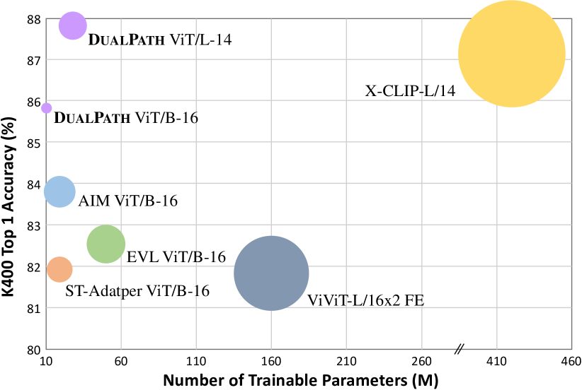
Figure 1: Performance comparison on the Kinetics-400 [40] dataset. We depict the action recognition performance (vertical axis, %) with respect to the number of trainable parameters (horizontal axis). The size of circles indicates GFLOPs for inference.

Most recently, parameter-efficient transfer learning (PETL) methods [33, 27, 43, 66, 26, 34] have been proposed as an alternative to finetuning in the natural language processing area to adapt the large-scale language model, such as GPT series [59, 60, 8] and T5 [61], for each task. They have successfully attained comparable or even surpassing performance to full-tuning parameters by learning a small number of extra trainable parameters only while keeping the original parameters of the pretrained model frozen. Thanks to their effectiveness and simplicity, they have been extended to vision models by applying prompt-based methods [37, 3] and adapter-based methods [11, 54, 69]. They have efficiently adapted pretrained models to downstream tasks with significantly reduced tuning parameters, but most of these works mainly focus on transferring image models to image tasks [37, 3, 11, 54] and vision-language models to vision-language tasks [69]. Inspired by the advances of the prior arts, we raise two conceivable questions: (1) Is it possible to transfer the parameters of the image foundation model to another video domain? (2) Is it also possible the transferred model performs comparably to the carefully designed video models that take the spatiotemporal nature of the video into account?

While image models have demonstrated strong spatial context modeling capabilities [58, 36, 68, 84], video transformer models [1, 50, 62, 81] require a more complex architecture (e.g. 539 vs 48912 GFLOPs [62]) with a large number of parameters (e.g. 84M vs 876M parameters [81]) than ViT for temporal context reasoning. Therefore, the challenge in transferring image models for video understanding is to encode the temporal context of videos while leveraging the discriminative spatial context of the pretrained image models. A naive solution is to finetune image models on a video dataset by directly applying previous prompt-/adapter-based approaches [37, 3, 11, 54]. However, these approaches inevitably ignore the temporal context in videos because they bridge only the spatial contexts between image and video data.

In this paper, we propose a novel adapter-based dual-path parameter efficient tuning method for video understanding, namely DualPath, which consists of two distinct paths (spatial path and temporal path). For both paths, we freeze the pretrained image model and train only additional bottleneck adapters for tuning. The spatial path is designed to encode the spatial contexts that can be inferred from the appearance of individual frames with the minimum tuning of the pretrained image model. To reduce the computation burden, we sparsely use the frames with a low frame rate in the spatial path. The temporal path corresponds to the temporal context that should be encoded by grasping the dynamic relationship over several frames sampled with a high frame rate. Especially for two reasons, we construct a grid-like frameset that consists of consecutive low-resolution frames as an input of the temporal path: (i) preventing computational efficiency loss caused by calculating multiple frames simultaneously; (ii) precisely imitating the ViT’s ability for extrapolating global dependencies between input tokens. To compare our DualPath with existing methods broadly, we implement several baselines with a unified perspective on recent domain-specific PETL approaches [11, 37, 54]. Extensive experiments on several action recognition benchmarks [40, 41, 24, 44] demonstrate the effectiveness and high efficiency of our DualPath, achieving comparable and even better performance than the baselines and prior video models [19, 45, 42, 7, 1, 50, 81, 62, 73, 23]. We achieve these results with extremely low computational costs for both training and inference, as demonstrated in Fig. 1.

2 Related Work

Pretraining vision models. To address the burdens of collecting large-scale labeled datasets for supervised learning [16, 68, 84], self-supervised learning methods [29, 12, 25, 28, 13, 79] have been introduced to learn general-purpose visual representations from unlabeled data. Similarly, self-supervised learning methods for videos have also been proposed with large-scale unlabeled video/video-language data [56, 57, 21, 70, 80, 73, 67]. However, collecting even unlabeled video-language pairs is still quite costly compared to image-language pairs. In addition, pretraining video models require more computational power than images. We thus take advantage of the powerful pretrained image-based models for efficient video understanding.

Video action recognition. Action recognition is one of the most fundamental research topics for video understanding. Early works have been built upon convolution neural networks (CNNs) [10, 78, 22, 46, 71] to effectively infer the spatiotemporal context for action recognition. Since Vision Transformer (ViT) [18] has become a new paradigm in computer vision, transformers for video understanding have been actively studied by extending pretrained image models. The pretrained image transformers have been used to initialize the part of the video transformers [1, 7, 85, 81] or inflated to the video transformers [50]. While transformers have demonstrated superior performance on video action recognition, they require full finetuning on video datasets, making the training inefficient.

Parameter-efficient transfer learning (PETL). To address the memory and parameter inefficiency of full-/partial-finetuning, PETL has first introduced in natural language processing (NLP) [33, 27, 26, 34, 66, 43, 6]. The main objective of PETL is to attain comparable or surpassing performance on downstream tasks by finetuning with only a small number of trainable parameters. Although PETL approaches [37, 11, 3, 38, 54, 69, 11] have recently been studied in computer vision, they are ‘blind’ to other modalities such that image models are used for image tasks, and so are the other modalities. In contrast, we share the same objective as recent works for image-to-video transfer learning [47, 53, 55, 39], demonstrating the pretrained image models can be good video learners. However, they have several limitations in terms of parameter and computational efficiency. For example, [47] learned an extra decoder that contains 3D convolution layers and cross-frame attention, and [55] inserted additional depth-wise 3D convolution layers between the down-/up-projection layers of the adapter to perform temporal reasoning, inducing computational inefficiency. The most recent works [39, 53] require an additional text encoder branch as a classifier. Moreover, they have computational efficiency proportional to the temporal resolution. Our DualPath accomplishes more efficient spatiotemporal modeling while achieving higher performance.

3 Preliminaries and Baselines

3.1 Vision transformers for video

We briefly describe how to apply vision transformers for video understanding below. Following [72], given a set of $T$ frames in a video, we split each frame into $N$ patches of size $(P\times P)$ and tokenize them using a linear projection, such that

$${\mathbf{X}}_{t}=[\mathbf{x}_{t}\{\texttt{[CLS]}\},{\mathbf{x}}_{t}^{1},{\mathbf{x}}_{t}^{2},\cdots,{\mathbf{x}}_{t}^{N}]+\mathbf{p},$$ (1)

where ${\mathbf{X}}_{t}$ is a set of tokens for the $t$-th frame, and $\mathbf{x}_{t}\{\texttt{[CLS]}\}$ and $\mathbf{p}$ denote a learnable class token and a learned positional embedding respectively. We feed $(N+1)$ tokens of each frame to a sequence of $L$ transformer blocks, and the output of the $l$-th block $\mathbf{h}_{l,t}$ can be derived by the following equations:

$$\mathbf{z}_{l,t}=\mathbf{h}_{l-1,t} +\texttt{MHA}(\texttt{LN}(\mathbf{h}_{l-1,t})),$$ (2)

$$\mathbf{h}_{l,t}=\mathbf{z}_{l,t} +\texttt{MLP}(\texttt{LN}(\mathbf{z}_{l,t})),$$

where $\texttt{LN},\texttt{MHA}$, and MLP denote a layer normalization [2], multi-head attention [72], and a multilayer perceptron operation, respectively. We apply layer normalization to the learned $T$ class tokens from the final transformer block and treat them as a set of frame representations.

To take minimal temporal modeling into account the following baselines [37, 11, 54], we employ a temporal transformer block followed by a full-connected (FC) layer as a classifier for video action recognition, similar to [39]. We add learnable temporal positional embeddings $\mathbf{p}_{\text{temp}}$ to the frame representations (i.e., $\mathbf{x}_{t}\{\texttt{[cls]}\}\leftarrow\mathbf{x}_{t}\{\texttt{[cls]}\}+\mathbf{p}_{\text{temp}}$) and feed them into the transformer classifier. For the ST-adapter [55], we use a single FC layer as a classifier.

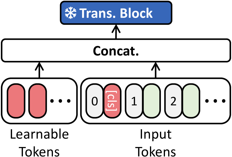
(a) VPT [37]

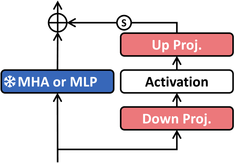
(b) Parallel Adapter [11]

(c) Serial Adapter [11]

(d) Prompt Block [54]

(e) ST-Adapter [55]

Figure 2: Baselines for image-to-video transfer learning. (a) Visual Prompt Tuning [37]; (b) Parallel adapter and (c) serial adapter [11]; (d) Pro-Tuning [54]; and (e) ST-Adapter [55].

3.2 Baselines

The objective of our work is to transfer the superiority of vision transformers pretrained on large-scale image datasets to the video domain through efficient finetuning with a small number of learnable parameters, while freezing the pretrained parameters. To compare with other methods, we generalize four recent PETL methods to the video domain only with the least possible transformation; (1) VPT [37] (2) AdaptFormer [11] (3) Pro-tuning [54] (4) ST-adapter [55]. The most of works have been originally proposed to adapt pretrained image models to downstream image tasks [37, 11, 54] and video models to video tasks [11], by learning visual prompt tokens [37], adapter blocks [11] and prompt prediction blocks [54]. Only the ST-adapter [55] has proposed image-to-video transfer learning. In this section, we describe baselines for image-to-video transfer learning in detail. For brevity, we leave out the subscripts in Eq. 2 and arouse them as needed. In addition, we represent the   learnable and   frozen parameters in red and blue colors, respectively.

Figure 3: Overall architecture of DualPath. The pretrained image transformer takes a grid-like frameset and $T_{s}$ frames as inputs. We learn the temporal and spatial contexts separately through two distinct paths. During training, we only update newly introduced adapters and the classifier while freezing the pretrained layers.

Visual prompt tuning (VPT) [37] prepends $K$ trainable prompt tokens to the input space of every transformer block while keeping pretrained parameters frozen. The input tokens for each transformer block can be written as:

$$\tilde{\mathbf{h}}=[{\hbox{\pagecolor{red!20}\vphantom{\parbox[c]{7.11317pt}{\rule{7.11317pt}{7.96674pt}}}{$\displaystyle\mathbf{e}$}}};\mathbf{h}],$$ (3)

where ${\hbox{\pagecolor{red!20}\vphantom{\parbox[c]{7.11317pt}{\rule{7.11317pt}{7.96674pt}}}{$\displaystyle\mathbf{e}$}}}\in\mathbb{R}^{K\times d}$ is a set of trainable visual prompt tokens and $d$ is a channel dimension of the original token.

AdaptFormer [11] learns a trainable bottleneck module [33, 27]. The intermediate feature $\mathbf{z}$ in Eq. 2 of each transformer block is fed into the AdapterMLP that consists of the original MLP layers and a bottleneck structure (parallel adapter in Fig. 2(b)). The output of the AdaptFormer block can be formulated by:

$$\tilde{\mathbf{z}} =\sigma({\hbox{\pagecolor{blue!20}\vphantom{\parbox[c]{7.11317pt}{\rule{7.11317pt}{7.96674pt}}}{$\displaystyle\texttt{LN}$}}}(\mathbf{z})\cdot{\hbox{\pagecolor{red!20}\vphantom{\parbox[c]{7.11317pt}{\rule{7.11317pt}{7.96674pt}}}{$\displaystyle\mathbf{W}_{\text{down}}$}}})\cdot{\hbox{\pagecolor{red!20}\vphantom{\parbox[c]{7.11317pt}{\rule{7.11317pt}{7.96674pt}}}{$\displaystyle\mathbf{W}_{\text{up}}$}}},$$ (4)

$$\mathbf{h} =\mathbf{z}+{\hbox{\pagecolor{blue!20}\vphantom{\parbox[c]{7.11317pt}{\rule{7.11317pt}{7.96674pt}}}{$\displaystyle\texttt{MLP}$}}}({\hbox{\pagecolor{blue!20}\vphantom{\parbox[c]{7.11317pt}{\rule{7.11317pt}{7.96674pt}}}{$\displaystyle\texttt{LN}$}}}(\mathbf{z}))+s\cdot\tilde{\mathbf{z}},$$

where ${\hbox{\pagecolor{red!20}\vphantom{\parbox[c]{7.11317pt}{\rule{7.11317pt}{7.96674pt}}}{$\displaystyle\mathbf{W}_{\text{down}}$}}},{\hbox{\pagecolor{red!20}\vphantom{\parbox[c]{7.11317pt}{\rule{7.11317pt}{7.96674pt}}}{$\displaystyle\mathbf{W}_{\text{up}}$}}}$ are trainable down- and up-projection matrices, $\sigma(\cdot)$ is an activation function, and $s$ is a scaling factor.

Pro-tuning [54] predicts task-specific vision prompts $\mathbf{v}$ from the output of each transformer block using consecutive 2D convolution layers. The output of each block is reshaped as $\mathbb{R}^{P\times P\times C}$ to apply 2D convolutions and the final representation is derived by adding $\mathbf{v}$ and $\mathbf{h}$:

$$\mathbf{v}=\texttt{Reshape}(\sigma( {\hbox{\pagecolor{red!20}\vphantom{\parbox[c]{7.11317pt}{\rule{7.11317pt}{7.96674pt}}}{$\displaystyle\texttt{Conv2d}$}}}(\texttt{Reshape}(\mathbf{h})))),$$ (5)

$$\tilde{\mathbf{h}} =\mathbf{h}+\mathbf{v},$$

where   Conv2D consists of $1\times 1$ convolution layer followed by $5\times 5$ depth-wise convolution [14] and $1\times 1$ convolution.

ST-adapter [55] inserts a depth-wise 3D convolution layer between the down-projection layer and the activation function of the adapter. Different from the conventional adapters (e.g. AdaptFormer [11]), the ST-adapter takes tokens for all frames to enable the model to capture temporality in videos. The output of the ST-adapter can be represented as:

$$\tilde{\mathbf{z}}_{t} ={\hbox{\pagecolor{blue!20}\vphantom{\parbox[c]{7.11317pt}{\rule{7.11317pt}{7.96674pt}}}{$\displaystyle\texttt{LN}$}}}(\mathbf{z}_{t}),$$ (6)

$$\hat{\mathbf{z}}=\sigma({\hbox{\pagecolor{red!20}\vphantom{\parbox[c]{7.11317pt}{\rule{7.11317pt}{7.96674pt}}}{$\displaystyle\texttt{D}\text{-}\texttt{Conv3d}$}}}([ \tilde{\mathbf{z}}_{1}{\cdot}{\hbox{\pagecolor{red!20}\vphantom{\parbox[c]{7.11317pt}{\rule{7.11317pt}{7.96674pt}}}{$\displaystyle\mathbf{W}_{\text{down}}$}}},\cdots,\tilde{\mathbf{z}}_{T}{\cdot}{\hbox{\pagecolor{red!20}\vphantom{\parbox[c]{7.11317pt}{\rule{7.11317pt}{7.96674pt}}}{$\displaystyle\mathbf{W}_{\text{down}}$}}}])){\cdot}{\hbox{\pagecolor{red!20}\vphantom{\parbox[c]{7.11317pt}{\rule{7.11317pt}{7.96674pt}}}{$\displaystyle\mathbf{W}_{\text{up}}$}}},$$

$$\mathbf{h}_{t}=\mathbf{z}_{t}+ {\hbox{\pagecolor{blue!20}\vphantom{\parbox[c]{7.11317pt}{\rule{7.11317pt}{7.96674pt}}}{$\displaystyle\texttt{MLP}$}}}(\tilde{\mathbf{z}}_{t})+s\cdot\hat{\mathbf{z}}_{t},$$

where   D-Conv3d denotes the depth-wise 3D convolution layer. Note that the same down-projection matrix   $\displaystyle\mathbf{W}_{\text{down}}$ is applied to all tokens regardless of the frame index $t$.

We emphasize that most of the baselines [37, 11, 54] have not concerned with temporal modeling. Even though ST-Adapter [55] has employed depth-wise 3D convolution layers between linear projections, it results in high computational cost. To entirely leverage a simple and efficient architecture of the adapter [11], we incorporate the dual-path design into the pretrained image transformers.

4 Method

The dual-path design (also called two-stream) is well-known architecture in CNN-based models for video recognition [10, 65, 22]. They have commonly used an optical flow [10, 65] or multiple frames with a high temporal resolution [22] to capture rapidly changing motion. Despite the effectiveness of dual-path architecture, it has yet to be explored with the transformer due to high computational costs. In this work, we propose a novel PETL method, called DualPath, comprised of spatial and temporal path adaptation. To the best of our knowledge, our DualPath is the first attempt to explicitly build the two-stream architecture upon the transformer while maintaining the computational cost similar to the single-stream architecture. The overall framework is depicted in Fig. 3.

4.1 Spatial adaptation

Since the image foundation models have been trained on large amounts of web datasets, we can intuitively speculate that they might be powerful to encode the spatial context even in videos. In order to make the outstanding ability of spatial modeling to be more suitable for video understanding with a slight parameter tuning, we adopt two parallel adapters for MHA and MLP in each transformer block. The parallel adapters allow the model to learn the spatial context for action recognition from the appearance of target video data while maintaining the original contexts for object recognition.

Specifically, we sample $T_{S}$ frames from a video and tokenize each frame. Similar to Eq. 1, the set of spatial tokens $\mathbf{X}^{\text{SP}}_{t}$ includes the learnable positional encodings   $\displaystyle\mathbf{p}^{\text{SP}}$ and the spatial class token   $\displaystyle\mathbf{x}_{t}^{\text{SP}}\{\texttt{[CLS]}\}$. The spatial adaptation in the $l$-th transformer block can be formulated by the following equations:

$$\mathbf{z}_{l}^{\text{SP}}=\mathbf{h}_{l-1}^{\text{SP}} +{\hbox{\pagecolor{blue!20}\vphantom{\parbox[c]{7.11317pt}{\rule{7.11317pt}{7.96674pt}}}{$\displaystyle\texttt{MHA}$}}}({\hbox{\pagecolor{blue!20}\vphantom{\parbox[c]{7.11317pt}{\rule{7.11317pt}{7.96674pt}}}{$\displaystyle\texttt{LN}$}}}(\mathbf{h}_{l-1}^{\text{SP}}))+{\hbox{\pagecolor{red!20}\vphantom{\parbox[c]{7.11317pt}{\rule{7.11317pt}{7.96674pt}}}{$\displaystyle\texttt{Adapter}$}}}({\hbox{\pagecolor{blue!20}\vphantom{\parbox[c]{7.11317pt}{\rule{7.11317pt}{7.96674pt}}}{$\displaystyle\texttt{LN}$}}}(\mathbf{h}_{l-1}^{\text{SP}})),$$ (7)

$$\mathbf{h}_{l}^{\text{SP}}=\mathbf{z}_{l}^{\text{SP}} +{\hbox{\pagecolor{blue!20}\vphantom{\parbox[c]{7.11317pt}{\rule{7.11317pt}{7.96674pt}}}{$\displaystyle\texttt{MLP}$}}}({\hbox{\pagecolor{blue!20}\vphantom{\parbox[c]{7.11317pt}{\rule{7.11317pt}{7.96674pt}}}{$\displaystyle\texttt{LN}$}}}(\mathbf{z}_{l}^{\text{SP}}))+{\hbox{\pagecolor{red!20}\vphantom{\parbox[c]{7.11317pt}{\rule{7.11317pt}{7.96674pt}}}{$\displaystyle\texttt{Adapter}$}}}({\hbox{\pagecolor{blue!20}\vphantom{\parbox[c]{7.11317pt}{\rule{7.11317pt}{7.96674pt}}}{$\displaystyle\texttt{LN}$}}}(\mathbf{z}_{l}^{\text{SP}})),$$

where $\mathbf{h}_{0}^{\text{SP}}=[{\hbox{\pagecolor{red!20}\vphantom{\parbox[c]{7.11317pt}{\rule{7.11317pt}{7.96674pt}}}{$\displaystyle\mathbf{x}_{t}^{\text{SP}}\{\texttt{[CLS]}\}$}}},\mathbf{X}_{t}^{\text{SP}}]+{\hbox{\pagecolor{red!20}\vphantom{\parbox[c]{7.11317pt}{\rule{7.11317pt}{7.96674pt}}}{$\displaystyle\mathbf{p}^{\text{SP}}$}}}$. We average the set of the spatial [CLS] tokens from the final transformer block to obtain a global spatial representation $\mathbf{y}^{\text{SP}}$, such that,

$$\mathbf{y}^{\text{SP}}=\frac{1}{T_{S}}\sum_{t=1}^{T_{S}}\mathbf{x}_{t}^{\text{SP}}\{\texttt{[CLS]}\}.$$ (8)

Recent methods have discussed that a high frame rate only increases the computation volume and is unnecessary to understand the semantics of appearance [22, 9]. We thus sparsely sample $T_{S}$ frames with a low frame rate (e.g. 8 frames per clip).

4.2 Temporal adaptation

While spatial adaptation enables the models to take the spatial contexts in video data, the image models are still incapable of modeling the temporal dynamics. The key component that allows video transformers to model the solid temporal context is to learn relationships between local patches across frames in the video [7, 1]. To make image models capable of effectively establishing this component, we suggest a novel grid-like frameset transform technique that aggregates multiple frames into a unified grid-like frameset. Our grid-like frameset design is inspired by recent visual prompting research [5, 4]. It is simple yet surprisingly effective in imitating temporal modeling as spatial modeling and certainly reduces the computation. In each transformer block, we adopt two additional serial adapters for MHA and MLP, respectively.

More concretely, we sample $T$ frames from a video and scale them with factors of $w$ and $h$, such that the scaled frame size is $[W/w\times H/h\times 3]$. We stack $w\times h$ scaled frames according to temporal ordering and reshape a stacked frame to construct a set of frames in a grid form of the same size as the original frame (i.e., $[W\times H\times 3]$). Note that the total number of grid-like framesets is $T_{G}=T/wh$. The set of temporal tokens $\mathbf{X}_{g}^{\text{TP}}$ for the $g$-th frameset is obtained in the same way in Eq. 1 and combined with the learnable temporal class token   $\displaystyle\mathbf{x}_{g}^{\text{TP}}\{\texttt{[CLS]}\}$. Unlike the spatial adaptation, we use fixed 3D positional encodings [75], $\mathbf{p}^{\text{TP}}$, to the tokens to take the absolute temporal order and spatial positions of patches into account. The input transformation allows transformers to observe multiple frames at the same level. In experiments, we mainly construct a grid-like frameset from 16 original frames (i.e., scaling factors $w=h=4$) to take the computational efficiency and promising performance.

Whereas the parallel adapter is used in the spatial path, we sequentially append adapters to the top of MHA and MLP layers in each transformer block. Formally, temporal adaptation in the $l$-th block can be described as:

$$\mathbf{z}_{l}^{\text{TP}}=\mathbf{h}_{l-1}^{\text{TP}} +{\hbox{\pagecolor{red!20}\vphantom{\parbox[c]{7.11317pt}{\rule{7.11317pt}{7.96674pt}}}{$\displaystyle\texttt{Adapter}$}}}({\hbox{\pagecolor{blue!20}\vphantom{\parbox[c]{7.11317pt}{\rule{7.11317pt}{7.96674pt}}}{$\displaystyle\texttt{MHA}$}}}({\hbox{\pagecolor{blue!20}\vphantom{\parbox[c]{7.11317pt}{\rule{7.11317pt}{7.96674pt}}}{$\displaystyle\texttt{LN}$}}}(\mathbf{h}_{l-1}^{\text{TP}}))),$$ (9)

$$\mathbf{h}_{l}^{\text{TP}}=\mathbf{z}_{l}^{\text{TP}} +{\hbox{\pagecolor{red!20}\vphantom{\parbox[c]{7.11317pt}{\rule{7.11317pt}{7.96674pt}}}{$\displaystyle\texttt{Adapter}$}}}({\hbox{\pagecolor{blue!20}\vphantom{\parbox[c]{7.11317pt}{\rule{7.11317pt}{7.96674pt}}}{$\displaystyle\texttt{MLP}$}}}({\hbox{\pagecolor{blue!20}\vphantom{\parbox[c]{7.11317pt}{\rule{7.11317pt}{7.96674pt}}}{$\displaystyle\texttt{LN}$}}}(\mathbf{z}_{l}^{\text{TP}}))),$$

where $\mathbf{h}^{\text{TP}}_{0}=[{\hbox{\pagecolor{red!20}\vphantom{\parbox[c]{7.11317pt}{\rule{7.11317pt}{7.96674pt}}}{$\displaystyle\mathbf{x}_{g}^{\text{TP}}\{\texttt{[CLS]}\}$}}},\mathbf{X}_{g}^{\text{TP}}]+\mathbf{p}^{\text{TP}}$. Similar to spatial adaptation, a global temporal representation $\mathbf{y}^{\text{TP}}$ can be derived by averaging the set of the temporal [CLS] tokens from the final transformer block, i.e.,

$$\mathbf{y}^{\text{TP}}=\frac{1}{T_{G}}\sum_{g=1}^{T_{G}}\mathbf{x}_{g}^{\text{TP}}\{\texttt{[CLS]}\}.$$ (10)

For the final prediction, we concatenate the global spatial and temporal representations and feed them into the classifier with GeLU activation [31] between two FC layers.

(a) DualPath w/o TA

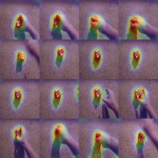
(b) DualPath w/ TA

Figure 4: Visualization of attention maps (a) without temporal adaptation (TA) and (b) with temporal adaptation for the action ’Spinning [something] that quickly stops spinning’ in SSv2 [24].

Method & Arch.	Pretrain	Model # Params	Trainable # Params	GFLOPs	R@1	R@5	Views
Full-tuning
SlowFast+NL [22]	-	60M	60M	7020	79.8	93.9	16$\times$3$\times$10
MViT-B [19]	-	37M	37M	4095	81.2	95.1	64$\times$3$\times$3
UniFormer-B [42]	IN-1K	50M	50M	3108	83.0	95.4	32$\times$4$\times$3
TimeSformer-L [7]	IN-21K	121M	121M	7140	80.7	94.7	64$\times$1$\times$3
ViViT-L/16$\times$2 FE [1]	IN-1K	311M	311M	3980	80.6	92.7	32$\times$1$\times$1
VideoSwin-L [50]	IN-21K	197M	197M	7248	83.1	95.9	32$\times$4$\times$3
MViTv2-L [45]	IN-21K	218M	218M	42420	86.1	97.0	32$\times$3$\times$5
MTV-L [81]	JFT	876M	876M	18050	84.3	96.3	32$\times$4$\times$3
TokenLearner-L/10 [62]	JFT	450M	450M	48912	85.4	96.3	64$\times$4$\times$3
ActionCLIP [73]	CLIP	142M	142M	16890	83.8	97.1	32$\times$10$\times$3
X-CLIP-L/14 [53]	CLIP	420M	420M	7890	87.1	97.6	8$\times$4$\times$3
Parameter Efficient Tuning
EVL [47] w/ ViT-L/14	CLIP	368M	59M	8088	87.3	-	32$\times$3$\times$1
ST-Adapter [55] w/ ViT-B/16	CLIP	93M	7M	1821	82.7	96.2	32$\times$3$\times$1
DualPath w/ ViT-B/16	CLIP	96M	10M	710	85.4	97.1	32$\times$3$\times$1
DualPath w/ ViT-L/14	CLIP	330M	27M	1868	87.7	97.8	32$\times$3$\times$1

Table 1: Performance comparisons for action recognition on the Kinetics-400 [40] dataset. Note that Views = #frames $\times$ #clips $\times$ #spatial.

4.3 Does a grid-like frameset really help to encode temporal context?

This work presents a new standpoint to perform video action recognition with the pretrained image transformer by transforming multiple frames into a unified grid-like frameset. However, it is still questionable whether the temporal path of DualPath can really capture the temporal context of videos. In this section, we provide some qualitative examples of the attention map. To validate the ability of precise temporal modeling, we sample videos from the SSv2 [24] dataset. Following [55], we depict the attention map of $\mathbf{x}_{g}^{\text{TP}}\{\texttt{[CLS]}\}$ from the final transformer block of the temporal path. As shown in Fig. 4, the model with the temporal adaptation (TA) of DualPath tends to concentrate on action-related regions, contrary to the model without TA that focuses on the irrelevant background. This result suggests that the temporal adaptation of DualPath strengthens the temporal modeling ability of the image model. More examples are shown in Fig. A1 of Appendix.

5 Experiment

5.1 Evaluation setup

Datasets. We evaluate the proposed method on four standard action recognition datasets, including the Kinetics-400 (K400) [40], HMDB51 [41], Something-something-v2 (SSv2) [24], and Diving-48 [44].

• Kinetics-400 (K400) contains about 240K training videos and 20K validation videos for 400 human action categories. Each video is trimmed to have a length of 10 seconds. While the K400 dataset provides a wide range of categories, they are known to be highly biased in spatial appearance [64].

• Somthing-something-v2 (SSv2) is a more challenging dataset since they require strong temporal modeling [64]. They contain about 168.9K training videos and 24.7K validation videos for 174 classes.

• HMDB51 is a small dataset that provides about 7K videos of 51 action categories. We use all three splits, each split of which consists of 3570 and 1530 videos for training and evaluation, respectively. We report the average accuracy for three splits.

• Diving-48 is a fine-grained diving action dataset. We use train-test split v2 that contains about 15K training videos and 2K validation videos of 48 diving actions. Since the action can not be determined by only the static representations (e.g. objects or background), stronger temporal modeling is required for this dataset.

Method & Arch.	Pretrain	Model #Params	Trainable #Params	GFLOPs	R@1	R@5	Views
Full-tuning
Full-tuning ViT-B/16 [18]	CLIP	86M	86M	419	44.0	77.0	8$\times$1$\times$3
Full-tuning ViT-L/14 [18]	CLIP	303M	303M	1941	48.7	77.5	8$\times$1$\times$3
TimeSformer-L [7]	IN-21K	121M	121M	7140	62.4	-	64$\times$1$\times$3
MTV-B [81]	IN-21K	310M	310M	4790	67.6	90.4	32$\times$4$\times$3
MViT-B [19]	K400	37M	37M	510	67.1	90.8	32$\times$1$\times$3
MViTv2-B [45]	K400	51M	51M	675	70.5	92.7	40$\times$1$\times$3
ViViT-L/16$\times$2 [1]	IN-21K/K400	311M	311M	11892	65.4	89.8	16$\times$4$\times$3
VideoSwin-B [50]	IN-21K/K400	89M	89M	963	69.6	92.7	32$\times$1$\times$1
Omnivore [23]	IN-21K/K400	-	-	-	71.4	93.5	32$\times$1$\times$3
MViTv2-B [45]	IN-21K/K400	213M	213M	8484	73.3	94.1	32$\times$1$\times$3
UniFormer-B [42]	IN-21K/K600	50M	50M	777	71.2	92.8	32$\times$1$\times$3
Parameter Efficient Tuning
VideoPrompt∗ [39] w/ ViT-B/16	CLIP	92M	6M	537	31.0	60.3	8$\times$1$\times$3
VPT [37] w/ ViT-B/16	CLIP	92M	6M	537	36.2	61.1	8$\times$1$\times$3
AdaptFormer [11] w/ ViT-B/16	CLIP	94M	8M	544	51.3	70.6	8$\times$1$\times$3
Pro-tuning [54] w/ ViT-B/16	CLIP	95M	9M	538	50.8	69.9	8$\times$1$\times$3
EVL [47] w/ ViT-L/14	CLIP	484M	175M	9641	66.7	-	32$\times$1$\times$3
ST-Adapter [55] w/ ViT-B/16	CLIP	97M	11M	1955	69.5	92.6	32$\times$3$\times$1
DualPath w/ ViT-B/16	CLIP	99M	13M	642	69.6	92.5	16$\times$1$\times$3
DualPath w/ ViT-B/16	CLIP	99M	13M	716	70.3	92.9	32$\times$1$\times$3
DualPath w/ ViT-B/16	CLIP	99M	13M	791	71.2	93.2	48$\times$1$\times$3
DualPath w/ ViT-L/14	CLIP	336M	33M	1713	70.2	92.7	16$\times$1$\times$3
DualPath w/ ViT-L/14	CLIP	336M	33M	1932	71.4	93.4	32$\times$1$\times$3
DualPath w/ ViT-L/14	CLIP	336M	33M	2151	72.2	93.7	48$\times$1$\times$3

Table 2: Performance comparisons for action recognition on the SSv2 [24] dataset. Note that we reproduce VideoPrompt [39] without the additional text branch for fair comparison (denoting with $*$).

Pretrained image backbone. We employ CLIP pretrained ViT-B/16 and ViT-L/14 as backbones. The results with Swin-B [49] are provided in Tab. A2 of the Appendix.

• ViT-B/16 [18] consists of 12 transformer blocks with 86M parameters and takes patches of size $16\times 16$ as inputs.

• ViT-L/14 [18], a larger model than ViT-B/16, contains 24 transformer blocks with 303M parameters. It takes $14\times 14$ patches as inputs.

Implementation details. For the K400, HMDB51, and Diving-48 datasets, we uniformly sample 8 frames (i.e., $T_{s}=8$) with the sampling interval 8 in the spatial path. In the temporal path, we uniformly sample 16, 32, and 48 frames with the sampling intervals 4, 2, and 1 to construct 1, 2, and 3 grid-like framesets (i.e., $T_{g}=1,2,3$), respectively. For the SSv2 dataset, we sample the same number of frames as in other datasets, but with a dynamic sampling interval to cover the whole video. Note that the frames for the spatial path are the subset of the temporal path frames. Please refer to more implementation details in Appendix A.

5.2 Comparison with state-of-the-art

In this section, we compare the proposed method with baselines [11, 37, 54, 55] in Sec. 3 and state-of-the-art video transformers [19, 42, 7, 1, 50, 45, 81, 62, 73, 53, 47] to demonstrate the effectiveness of the proposed method on four video action recognition datasets. Note that the number of frames of the spatial adaptation path of DualPath is fixed to 8 for all experiments, i.e., $T_{S}=8$.

Results on Kinetics-400. We report the results evaluated on K400 [40] in Tab. 1. We first compare the proposed method with state-of-the-art video models that are pretrained on the large-scale image dataset and fully finetuned on K400. In terms of memory and computational efficiency, video models require a huge number of parameters ($\sim$450M [62]) and computations ($\sim$48912 GFLOPs [62]). On the other hand, we require only 10M trainable parameters which are newly stored, and 710 GFLOPs for inference using 32 frames with ViT-B/16 [18] backbone. Compared to X-CLIP-L/14 [53] which leverages the additional text branch, our DualPath achieves state-of-the-art performance with ViT-L/14 backbone. The comparisons with parameter-efficient tuning methods [47, 55] show that our DualPath achieves higher performance while requiring much lower burdens in computations under the same conditions.

Results on Something-Something-v2. We present the performance comparisons on SSv2 [24] in Tab. 2. The results show that our DualPath with ViT-B/16 achieves comparable or better performance than the prior supervised video models [7, 81, 19, 1], requiring a much smaller number of trainable parameters and GFLOPs. Our DualPath with ViT-L/14 shows more competitive performance, outperforming most prior works [45, 42, 23]. The baselines [39, 37, 11, 54], which have relatively weak temporal modeling ability, show significantly poor performance, implying that strong temporal modeling is mandatory for the SSv2 dataset. The comparisons to the CLIP pretrained PET approaches [47, 55] with ViT-B/16 demonstrate the effectiveness and efficiency of DualPath, achieving higher performance (70.3 vs 69.5 [55]) with significantly low computations (716 vs 9641 [47] GFLOPs) using 32 frames. Thanks to the extreme computational efficiency, our DualPath comprises more competitive performance using 48 frames ($T_{G}=3$) with low computation requirements.

Method & Arch.	Classifier	Params	HMDB51
Full-tuning w/ ViT-B/16 [18]	Lin.	86M	59.4
Linear w/ ViT-B/16	Lin.	0.1M	61.2
VPT [37] w/ ViT-B/16	Trans.	7M	62.4
AdaptFormer [11] w/ ViT-B/16	Trans.	8M	63.7
Pro-tuning [54] w/ ViT-B/16	Trans.	9M	63.3
VideoPrompt [39] w/ ViT-B/16	Trans.	6M	66.4
ST-Adapter∗ [55] w/ ViT-B/16	Lin.	7M	65.9
DualPath w/ ViT-B/16	MLPs.	10M	75.6

Table 3: Performance comparisons for action recognition on the HMDB51 [41] dataset with the CLIP pretrained ViT-B/16 [58]. We report the type of classifier and the number of learnable parameters for baselines and ours. Lin. and Trans. denote the linear classifier and temporal transformer, respectively. Our DualPath uses two MLP layers as the classifier. Note that we reproduce ST-Adapter [55] for fair comparison in terms of the pretrained dataset (denoting with ${*}$).

Method & Arch.	Pretrain	Params	Diving48
Supervised
TimeSformer-L [7]	IN-21K	121M	81.0
VideoSwin-B [50]	IN-21K	88M	81.9
SIFAR-B-14 [20]	IN-21K	87M	87.3
ORViT [32]	IN-21K	160M	88.0
Parameter Efficient Tuning
DualPath w/ ViT-B/16	CLIP	10M	88.7

Table 4: Performance comparisons for action recognition on the Diving-48 [44] dataset. We report the pretrained dataset, the number of learnable parameters (M) for each method, and the accuracy.

Results on HMDB51. In Tab. 3, we compare the results with baselines [37, 11, 54, 39, 55] on HMDB51 [41] that dominantly requires strong spatial modeling for action recognition. Surprisingly, our DualPath significantly outperforms baselines by large margins. This result demonstrates DualPath fully capitalizes on the exceptional spatial modeling ability of the pretrained image model for action recognition. The comparison with VideoPrompt [39] that uses the additional text branch demonstrates the effectiveness of DualPath, improving 9.2% performance improvement.

Results on Diving-48. Tab. 4 shows performance comparisons on Diving-48 [44] that requires fine-grained action recognition. Our DualPath consistently outperforms all video models with only 10M trainable parameters. Particularly, we obtain a better performance than ORViT [32] which utilizes the additional tracking model. It indicates the utility of DualPath in fine-grained action recognition and the superiority of temporal modeling of DualPath.

5.3 Components analysis

Impact of dual-path. In the top panel of Tab. 5, we train the model by ablating each path and evaluate the performance on SSv2. Without the temporal path (DualPath w/o TA), the performance is significantly degraded despite using a larger number of frames ($T_{S}\,$=$\,16$ vs $8$). Without the spatial path (DualPath w/o SA), we can obtain slightly better performance than the result without the temporal adaptation. Since the SSv2 requires strong temporal modeling, we speculate that two ablation studies show comparison results. However, it still shows a substantial performance gap compared to the full model of DualPath, demonstrating the effectiveness of the dual-path design.

Frame rates in spatial path. In the middle panel of Tab. 5, we analyze the effect according to the number of frames used in the spatial path. The temporal path identically uses 16 frames to construct a grid-like frameset, and frames used in the spatial path are sampled from such 16 frames. A large number of $T_{S}$ slightly improves performance, however, requires more computational costs. Considering the performance improvement compared to the computation increase, we mainly set $T_{S}$ to 8.

Number of frames in grid. We scale down original frames with scaling factors $w$ and $h$ to construct grid-like framesets. These factors thus determine the number of frames the model observes within one grid-like frameset. While a large value of factors increases the temporal resolution, the information of each frame is inevitably reduced. For example, the original frame is scaled down to the size of $28\times 28$ with $w\,$=$\,h\,$=$\,8$. Meanwhile, a small value of factors retains richer information from the original frame, however, makes the temporal resolution small. As shown in the bottom panel of Tab. 5, we attain the best performance with $w\,$=$\,h\,$=$\,4$.

Method	Params	GFLOPs	SSv2	Views
Effectiveness of Each Path
DualPath w/o TA	5M	1016	53.7	16$\times$3$\times$1
DualPath w/o SA	8M	134	55.1	16$\times$3$\times$1
Effectiveness of $T_{S}$
$T_{S}=8$	13M	642	69.3	16$\times$3$\times$1
$T_{S}=12$	13M	896	69.6	16$\times$3$\times$1
$T_{S}=16$	13M	1150	69.8	16$\times$3$\times$1
Effectiveness of scaling factors
$w$=$h$=$2\;(T_{G}$=$16)$	13M	1752	66.4	64$\times$3$\times$1
$w$=$h$=$4\;(T_{G}$=$4)$	13M	864	71.8	64$\times$3$\times$1
$w$=$h$=$8\;(T_{G}$=$1)$	13M	642	61.5	64$\times$3$\times$1
DualPath	13M	642	69.3	16$\times$3$\times$1

Table 5: Performance with respect to variants of the components.

6 Conclusion and Future Work

In this paper, we have introduced the novel image-to-video transfer learning approach, DualPath. By incorporating a dual-path design into image transformers, DualPath adapts image models to the video task (i.e., action recognition) with a small number of trainable parameters. The spatial path adaptation strengthens the inherent spatial context modeling of the pretrained image transformers for video data. The temporal path adaptation transforms multiple frames into a unified grid-like frameset, enabling the image model to capture relationships between frames. We appropriately employ the bottlenecked adapters in each path to adapt the pretrained features to target video data. In addition, we present several baselines transforming recent PETL approaches [37, 11, 54] for image-to-video adaptation. Experimental results demonstrated the superiority of the dual-path design and the grid-like frameset prompting, outperforming several baselines and supervised video models.

There are many possible directions for future work, encompassing cross-domain transfer learning. While we have explored image-to-video transfer learning, large foundation vision-language models are available. It would also be interesting to expand the superior pretrained 2D knowledge to 3D spatial modeling [76]. We hope our study will foster research and provide a foundation for cross-domain transfer learning.

Acknowledgement. This research was supported by the Yonsei Signature Research Cluster Program of 2022 (2022-22-0002) and the KIST Institutional Program (Project No.2E31051-21-203). This research was supported by the National Research Foundation of Korea (NRF) grant funded by the Korea government (MSIP) (NRF2021R1A2C2006703).

Appendix

Components	K400 [40]	SSv2 [24]	HMDB51 [41]	Diving-48 [44]
Adapter
# Adapters per block	4 (2 SP, 2 TP)	5 (2 SP, 3 TP)	4 (2 SP, 2 TP)	4 (2 SP, 2 TP)
Adapter bottleneck width	128	128	128	128
Optimizer (AdamW [52], Cosine scheduler [51])
Learning rate	3e-4	5e-4	1e-4	3e-4
Weight Decay	5e-2	5e-2	2e-2	3e-2
Batch size	64	128	128	128
Data configuration
Training crop size	224	224	224	224
Frame sampling rate ($T_{S}$)	16 for $T_{S}=8$	16 for $T_{S}=8$	16 for $T_{S}=8$	16 for $T_{S}=8$
Frame sampling rate ($T_{G}$)	8 for $T_{G}=1$ 4 for $T_{G}=2$ 2 for $T_{G}=3$	Dynamic sampling	8 for $T_{G}=1$ 4 for $T_{G}=2$ 2 for $T_{G}=3$	8 for $T_{G}=1$ 4 for $T_{G}=2$ 2 for $T_{G}=3$
RandAugment [15]	✓	✓	✓	✓
Random erase [86]	✗	✓	✓	✗
Inference configuration
Testing views (temporal$\times$spatial)	3 $\times$1	1$\times$3	2$\times$3	1$\times$1

Table A1: Implementation details of DualPath.

In this document, we include supplementary materials for “Dual-path Adaptation from Image to Video Transformers”. We first provide more concrete implementation details (Sec. A), and additional experimental results (Sec. B), including the results using a different backbone and ablation study for the resolution of the grid-like frameset. Finally, we visualize more attention maps from each path to complement the effectiveness of the proposed method (Sec. C).

Appendix A Implementation Details

We add parallel adapters in the spatial path and serial adapters in the temporal path to every transformer block. In our adapter, the dimension of the bottlenecked embedding is 128. Following prior work [11], $\mathbf{W}_{\text{down}}$ is initialized with Kaiming Normal [30] and $\mathbf{W}_{\text{up}}$ with zero initialization. For the SSv2 [24] dataset, we additionally insert one adapter before the multi-head attention layer in the temporal path for more robust temporal modeling. The experimental configurations according to the datasets are presented in Tab. A1.

Appendix B Additional Results

B.1 Results with Swin-B

Method & Arch.	Pretrain	Model # Params	Trainable # Params	GFLOPs	SSv2	HMDB51
Full-tuning w/ Swin-B [49]	IN-21K	88M	88M	124	44.3	61.2
ST-Adapter [55] w/ Swin-B	IN-21K	95M	7M	385	65.1	-
DualPath w/ ViT-B/16	CLIP	99M	13M	642	69.3	75.6
DualPath w/ ViT-B/16	IN-21K	99M	13M	642	64.7	70.5
DualPath w/ Swin-B	IN-21K	97M	11M	287	67.8	75.2

Table A2: Performance comparisons for action recognition on the SSv2 [24] and HMDB51 [41] dataset with different backbones and pretraining datasets.

Method	# Frames	K400 R@1$\uparrow$	Training GPU Hours $\downarrow$	Throughput (V/s) $\uparrow$	Inference Latency (ms) $\downarrow$
Uniformer-B [42]	32	82.9	5000	3.42	314.58
EVL w/ ViT-B [47]	8	82.9	60	25.53	102.88
DualPath w/ ViT-B	16	85.4	31	64.21	15.58

Table A3: Training and inference efficiency comparisons. All models are evaluated using V100-32G, following EVL [47].

Resolution	SSv2		HMDB51
	GFLOPs	R@1	GFLOPs	R@1
224$\times$224 w/ 16 frames	642	69.3	612	75.6
448$\times$448 w/ 16 frames	846	70.5	816	75.8
896$\times$896 w/ 16 frames	1694	71.6	1632	76.4
224$\times$224 w/ 48 frames	791	71.2	778	76.3

Table A4: Performance comparisons for action recognition on the SSv2 [24] and HMDB51 [41] dataset according to the resolution of the grid-like frameset.

Our DualPath can be applied to other transformer-based pretrained image models. We conduct additional experiments with Swin-B [49, 48] transformer pretrained on the ImageNet-21K [16]. The Swin-B contains 24 Swin transformer blocks with 88M parameters, requiring fewer GFLOPs than ViT-B/16 [18]. Each block consists of window-based and shifted window-based self-attention layers. As in the ViT backbones, we add parallel adapters in the spatial path and serial adapters in the temporal path to every Swin transformer block. Note that adapters are attached to only window-based self-attention layers while not adapting shifted window-based self-attention layers. For the SSv2 dataset, we use an additional adapter before the multi-head attention layer of the temporal path similar to the ViT backbones. The dimension of the bottlenecked embedding is set to 128.

Tab. A2 provides the experimental results of DualPath with Swin-B [49, 48] on the SSv2 [24] and HMDB51 [41] datasets. Although the comparisons between ViT-B/16 and Swin-B backbones show the significantly low computation requirement of the Swin-B model (642 vs 287 GFLOPs with DualPath), we attain a comparable performance to the CLIP pretrained ViT-B/16. Compared to ST-Adapter [55] with Swin-B, the results consistently demonstrate the effectiveness of DualPath over the backbone networks, showing a higher performance of 2.7% with Swin-B on the SSv2 benchmark.

B.2 Additional efficiency analysis

We additionally compare the methods with [47, 42] in terms of training step time, throughput, and inference latency, following [47]. For a fair comparison, we obtain all results using V100-32G with PyTorch-builtin mixed precision. The throughput is measured with the largest batch size before out-of-memory and the inference latency is measured with a batch size of 1. As shown in Tab. A3, DualPath takes about half of the training GPU hours and achieves ×2.5 more throughput and ×6.6 faster inference than EVL [47] under the same hardware condition.

B.3 Resolution of grid-like frameset

The grid-like frameset comprises a stack of 16 scaled frames to make the same size as the original frame ($224\times 224$). We investigate the effectiveness of the resolution of the grid-like frameset in this section. Note that the impact of scaling factors that determine the temporal resolution is demonstrated in Tab. 5 of the main paper.

Specifically, we set the scaling factors $w$ and $h$ to 1, 2, and 4 while maintaining the temporal resolution as 16 such that the resolution of the grid-like frameset is $896\times 896$, $448\times 448$, and $224\times 224$, respectively. The backbone (ViT-B/16) is identically used and uniformly sampled 8 frames are used in the spatial path. Following [55], we sample one clip cropped into three different spatial views on SSv2 [24] (i.e., total of 3 clips) at test time. For HMDB51 [41], two clips sampled from a video are respectively cropped into three spatial views (i.e., a total of 6 clips). Since a high-resolution frameset contains more detailed information about the original frames, the highest performance is obtained with the $896\times 896$ size of the frameset in Tab. A4. However, the computational cost quadratically increases as the resolution of the grid-like frameset increases. When we use 48 frames (i.e., $T_{G}=3$) with the $224\times 224$ size of the frameset, competitive performance is achieved in both datasets. It supports the resolution choice of DualPath in terms of the trade-off between performance and computational cost.

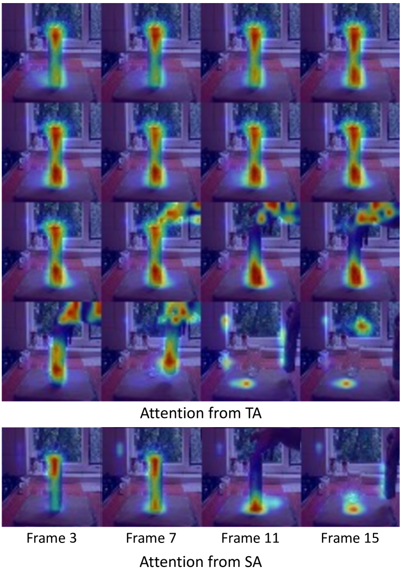
(a) Removing [something], revealing [something] behind

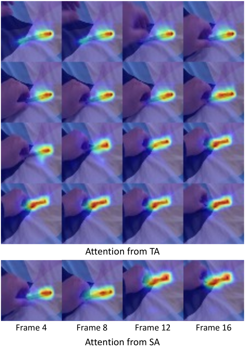
(b) Moving [something] up

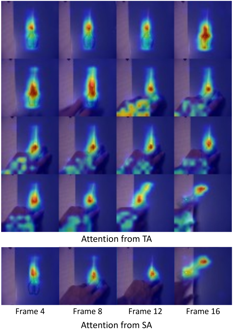
(c) Pushing [something] so that it falls off the table

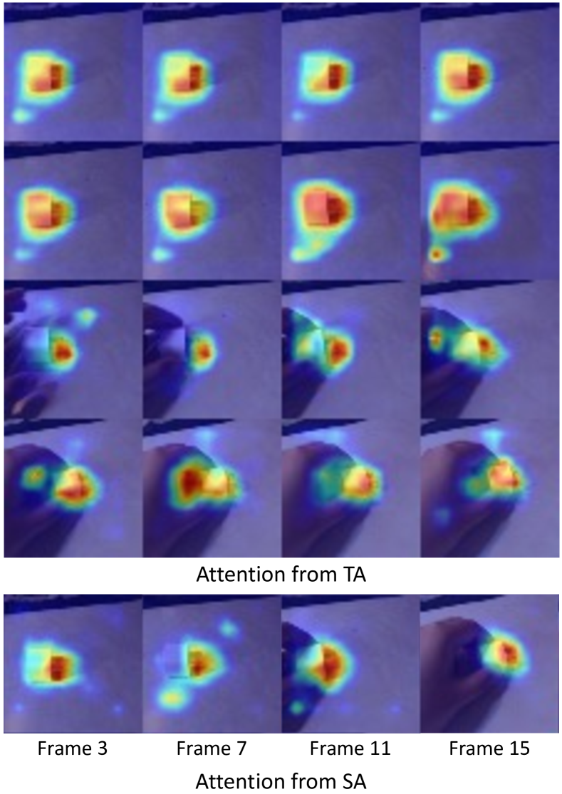
(d) Pushing [something] from left to right

Figure A1: Visualization of attention maps of each path for videos from the SSv2 [24] dataset.

Appendix C More Attention Visualization of DualPath

The additional attention visualization is illustrated in Fig. A1. We depict the attention maps of $\mathbf{x}_{t}^{\text{SP}}\{\texttt{[CLS]}\}$ and $\mathbf{x}_{g}^{\text{TP}}\{\texttt{[CLS]}\}$ from the final transformer block of each path. All videos are sampled from the SSv2 [24] dataset and ViT-B/16 is used as the backbone. While we use 8 frames in the spatial path, the attention maps corresponding to only 4 frames are displayed for visibility. Interestingly, the results show that the model trained with DualPath is capable of focusing on dynamic action-related regions in both adaptation paths. As exemplified in Fig. 1(a) and Fig. 1(c), $\mathbf{x}_{t}^{\text{SP}}\{\texttt{[CLS]}\}$ of the spatial path tends to focus on action-related objects, and $\mathbf{x}_{g}^{\text{TP}}\{\texttt{[CLS]}\}$ of the temporal path concentrates on action-related movements. Therefore, the two paths complement each other, leading to spatiotemporal modeling.

References

- [1] Anurag Arnab, Mostafa Dehghani, Georg Heigold, Chen Sun, Mario Lučić, and Cordelia Schmid. Vivit: A video vision transformer. In ICCV, 2021.
- [2] Jimmy Lei Ba, Jamie Ryan Kiros, and Geoffrey E. Hinton. Layer normalization. arXiv preprint: arXiv:1607.06450, 2016.
- [3] Hyojin Bahng, Ali Jahanian, Swami Sankaranarayanan, and Phillip Isola. Exploring visual prompts for adapting large-scale models. arXiv preprint: arXiv:2203.17274, 2022.
- [4] Hyojin Bahng, Ali Jahanian, Swami Sankaranarayanan, and Phillip Isola. Exploring visual prompts for adapting large-scale models. arXiv preprint: arXiv:2203.17274, 2022.
- [5] Amir Bar, Yossi Gandelsman, Trevor Darrell, Amir Globerson, and Alexei A. Efros. Visual prompting via image inpainting. arXiv preprint: arXiv:2209.00647, 2022.
- [6] Elad Ben-Zaken, Shauli Ravfogel, and Yoav Goldberg. Bitfit: Simple parameter-efficient fine-tuning for transformer-based masked language-models. In ACL, 2022.
- [7] Gedas Bertasius, Heng Wang, and Lorenzo Torresani. Is space-time attention all you need for video understanding? In ICML, 2021.
- [8] Tom B. Brown, Benjamin Mann, Nick Ryder, Melanie Subbiah, Jared Kaplan, Prafulla Dhariwal, Arvind Neelakantan, Pranav Shyam, Girish Sastry, Amanda Askell, Sandhini Agarwal, Ariel Herbert-Voss, Gretchen Krueger, Tom Henighan, Rewon Child, Aditya Ramesh, Daniel M. Ziegler, Jeffrey Wu, Clemens Winter, Christopher Hesse, Mark Chen, Eric Sigler, Mateusz Litwin, Scott Gray, Benjamin Chess, Jack Clark, Christopher Berner, Sam McCandlish Alec Radford, Ilya Sutskever, and Dario Amodei. Language models are few-shot learners. In NeurIPS, 2020.
- [9] Shyamal Buch, Cristóbal Eyzaguirre, Adrien Gaidon, Jiajun Wu, Li Fei-Fei, and Juan Carlos Niebles. Revisiting the “videos” in video-language understanding. In CVPR, 2022.
- [10] João Carreira and Andrew Zisserman. Quo vadis, action recognition? a new model and the kinetics dataset. In CVPR, 2017.
- [11] Shoufa Chen, Chongjian Ge, Zhan Tong, Jiangliu Wang, Yibing Song, Jue Wang, and Ping Luo. Adaptformer: Adapting vision transformers for scalable visual recognition. In NeurIPS, 2022.
- [12] Ting Chen, Simon Kornblith, Mohammad Norouzi, and Geoffrey Hinton. A simple framework for contrastive learning of visual representations. In ICML, 2020.
- [13] Xinlei Chen, Saining Xie, and Kaiming He. An empirical study of training self-supervised vision transformers. In ICCV, 2021.
- [14] François Chollet. Xception: Deep learning with depthwise separable convolutions. In CVPR, 2017.
- [15] Ekin Dogus Cubuk, Barret Zoph, Jon Shlens, and Quoc Le. Randaugment: Practical automated data augmentation with a reduced search space. In NeurIPS, 2020.
- [16] Jia Deng, Wei Dong, Richard Socher, Li-Jia Li, Kai Li, and Li Fei-Fei. Imagenet: A large-scale hierarchical image database. In CVPR, 2009.
- [17] Xiaoyi Dong, Jianmin Bao, Dongdong Chen, Weiming Zhang, Nenghai Yu, Lu Yuan, Dong Chen, and Baining Guo. Cswin transformer: A general vision transformer backbone with cross-shaped windows. In CVPR, 2022.
- [18] Alexey Dosovitskiy, Lucas Beyer, Alexander Kolesnikov, Dirk Weissenborn, Xiaohua Zhai, Thomas Unterthiner, Mostafa Dehghani, Matthias Minderer, Georg Heigold, Sylvain Gelly, Jakob Uszkoreit, and Neil Houlsby. An image is worth 16x16 words: Transformers for image recognition at scale. In ICML, 2021.
- [19] Haoqi Fan, Bo Xiong, Karttikeya Mangalam, Yanghao Li, Zhicheng Yan, Jitendra Malik, and Christoph Feichtenhofer. Multiscale vision transformers. In ICCV, 2021.
- [20] Quanfu Fan, Chun-Fu (Richard) Chen, and Rameswar Panda. Can an image classifier suffice for action recognition? In ICLR, 2022.
- [21] Christoph Feichtenhofer, Haoqi Fan, Yanghao Li, and Kaiming He. Masked autoencoders as spatiotemporal learners. arXiv preprint: arXiv:2205.09113, 2022.
- [22] Christoph Feichtenhofer, Haoqi Fan, Jitendra Malik, and Kaiming He. Slowfast networks for video recognition. In ICCV, 2019.
- [23] Rohit Girdhar, Mannat Singh, Nikhila Ravi, Laurens van der Maaten, Armand Joulin, and Ishan Misra. Omnivore: A single model for many visual modalities. In CVPR, 2022.
- [24] Raghav Goyal, Samira Ebrahimi Kahou, Vincent Michalski, Joanna Materzyńska, Susanne Westphal, Heuna Kim, Valentin Haenel, Ingo Fruend, Peter Yianilos, Moritz Mueller-Freitag, Florian Hoppe, Christian Thurau, Ingo Bax, and Roland Memisevic. The “something something” video database for learning and evaluating visual common sense. In ICCV, 2017.
- [25] Jean-Bastien Grill, Florian Strub, Florent Altché, Corentin Tallec, Pierre H. Richemond, Elena Buchatskaya, Carl Doersch, Bernardo Avila Pires, Zhaohan Daniel Guo, Mohammad Gheshlaghi Azar, Bilal Piot, Koray Kavukcuoglu, Rémi Munos, and Michal Valko. Bootstrap your own latent: A new approach to self-supervised learning. In NeurIPS, 2020.
- [26] Demi Guo, Alexander M. Rush, and Yoon Kim. Parameter-efficient transfer learning with diff pruning. In ACL, 2021.
- [27] Junxian He, Chunting Zhou, Xuezhe Ma, Taylor Berg-Kirkpatrick, and Graham Neubig. Towards a unified view of parameter-efficient transfer learning. In ICLR, 2022.
- [28] Kaiming He, Xinlei Chen, Saining Xie, Yanghao Li, Piotr Dollár, and Ross Girshick. Masked autoencoders are scalable vision learners. In CVPR, 2022.
- [29] Kaining He, Haoqi Fan, Yuxin Wu, Saining Xie, and Ross Girshick. Momentum contrast for unsupervised visual representation learning. In CVPR, 2020.
- [30] Kaiming He, Xiangyu Zhang, Shaoqing Ren, and Jian Sun. Delving deep into rectifiers: Surpassing human-level performance on imagenet classification. In ICCV, 2015.
- [31] Dan Hendrycks and Kevin Gimpel. Gaussian error linear units (gelus). arXiv preprint: arXiv:1606.08415, 2016.
- [32] Roei Herzig, Elad Ben-Avraham, Karttikeya Mangalam, Amir Bar, Gal Chechik, Anna Rohrbach, Trevor Darrell, and Amir Globerson. Object-region video transformers. In CVPR, 2022.
- [33] Neil Houlsby, Andrei Giurgiu, Stanisław Jastrzȩbski, Bruna Morrone, Quentin de Laroussilhe, Andrea Gesmundo, Mona Attariyan, and Sylvain Gelly. Parameter-efficient transfer learning for nlp. In ICML, 2019.
- [34] Edward J. Hu, Yelong Shen, Phillip Wallis, Zeyuan Allen-Zhu, Yuanzhi Li, Shean Wang, Lu Wang, and Weizhu Chen. Lora: Low-rank adaptation of large language models. In ICLR, 2022.
- [35] Shuiwang Ji, Wei Xu, Ming Yang, and Kai Yu. 3d convolutional neural networks for human action recognition. In ICML, 2010.
- [36] Chao Jia, Yinfei Yang, Ye Xia, Yi-Ting Chen, Zarana Parekh, Hieu Pham, Quoc V. Le, Yunhsuan Sung, Zhen Li, and Tom Duerig. Scaling up visual and vision-language representation learning with noisy text supervision. In ICML, 2021.
- [37] Menglin Jia, Luming Tang, Bor-Chun Chen, Claire Cardie1, Serge Belongie, Bharath Hariharan, and Ser-Nam Lim. Visual prompt tuning. In ECCV, 2022.
- [38] Shibo Jie and Zhi-Hong Deng. Convolutional bypasses are better vision transformer adapters. arXiv preprint. arXiv:2207.07039, 2022.
- [39] Chen Ju, Tengda Han, Kunhao Zheng, Ya Zhang, and Weidi Xie. Prompting visual-language models for efficient video understanding. In ECCV, 2022.
- [40] Will Kay, Joao Carreira, Karen Simonyan, Brian Zhang, Chloe Hillier, Sudheendra Vijayanarasimhan, Fabio Viola, Tim Green, Trevor Back, Paul Natsev, Mustafa Suleyman, and Andrew Zisserman. The kinetics human action video dataset. arXiv preprint: arXiv:1705.06950, 2017.
- [41] Hildegard Kuehne, Hueihan Jhuang, Estíbaliz Garrote, Tomaso Poggio, and Thomas Serre. Hmdb: A large video database for human motion recognition. In ICCV, 2011.
- [42] Kunchang Li, YaliWang, Gao Peng, Guanglu Song, Yu Liu, Hongsheng Li, and Yu Qiao. Uniformer: Unified transformer for efficient spatial-temporal representation learning. In ICLR, 2021.
- [43] Xiang Lisa Li and Percy Liang. Prefix-tuning: Optimizing continuous prompts for generation. In ACL, 2021.
- [44] Yingwei Li, Yi Li, and Nuno Vasconcelos. Resound: Towards action recognition without representation bias. In ECCV, 2018.
- [45] Yanghao Li, Chao-Yuan Wu, Haoqi Fan, Karttikeya Mangalam, Bo Xiong, Jitendra Malik, and Christoph Feichtenhofer. Mvitv2: Improved multiscale vision transformers for classification and detection. In CVPR, 2022.
- [46] Ji Lin, Chuang Gan, and Song Han. Tsm: Temporal shift module for efficient video understanding. In ICCV, 2019.
- [47] Ziyi Lin, Shijie Geng, Renrui Zhang, Peng Gao, Gerard de Melo, Xiaogang Wang, Jifeng Dai, Yu Qiao, and Hongsheng Li. Frozen clip models are efficient video learners. In ECCV, 2022.
- [48] Ze Liu, Han Hu, Yutong Lin, Zhuliang Yao, Zhenda Xie, Yixuan Wei, Jia Ning, Yue Cao, Zheng Zhang, Li Dong, Furu Wei, and Baining Guo. Swin transformer v2: Scaling up capacity and resolution. In CVPR, 2022.
- [49] Ze Liu, Yutong Lin, Yue Cao, Han Hu, Yixuan Wei, Zheng Zhang, Stephen Lin, and Baining Guo. Swin transformer: Hierarchical vision transformer using shifted windows. In ICCV, 2021.
- [50] Ze Liu, Jia Ning, Yue Cao, Yixuan Wei, Zheng Zhang, Stephen Lin, and Han Hu. Video swin transformer. In CVPR, 2022.
- [51] Ilya Loshchilov and Frank Hutter. Sgdr: Stochastic gradient descent with warm restarts. In ICLR, 2017.
- [52] Ilya Loshchilov and Frank Hutter. Decoupled weight decay regularization. In ICLR, 2019.
- [53] Bolin Ni, Houwen Peng, Minghao Chen, and Songyang Zhang. Expanding language-image pretrained models for general video recognition. In ECCV, 2022.
- [54] Xing Nie, Bolin Ni, Jianlong Chang, Gaomeng Meng, Chunlei Huo, Zhaoxiang Zhang, Shiming Xiang, Qi Tian, and Chunhong Pan. Pro-tuning: Unified prompt tuning for vision tasks. arXiv preprint: arXiv:2207.14381, 2022.
- [55] Junting Pan, Ziyi Lin, Xiatian Zhu, Jing Shao, and Hongsheng Li. St-adapter: Parameter-efficient image-to-video transfer learning for action recognition. In NeurIPS, 2022.
- [56] Tian Pan, Yibing Song, Tianyu Yang, Wenhao Jiang, and Wei Liu. Videomoco: contrastive video representation learning with temporally adversarial examples. In CVPR, 2021.
- [57] Jungin Park, Jiyoung Lee, Ig-Jae Kim, and Kwanghoon Sohn. Probabilistic representations for video contrastive learning. In CVPR, 2022.
- [58] Alec Radford, Jong Wook Kim, Chris Hallacy, Aditya Ramesh, Gabriel Goh, Sandhini Agarwal, Girish Sastry, Amanda Askell, Pamela Mishkin, Jack Clark, Gretchen Krueger, and Ilya Sutskever. Learning transferable visual models from natural language supervision. In ICLR, 2021.
- [59] Alec Radford, Karthik Narasimhan, Tim Salimans, and Ilya Sutskever. Improving language understanding by generative pre-training. Technical report, OpenAI, 2018.
- [60] Alec Radford, Jeffrey Wu, Rewon Child, David Luan, Dario Amodei, and Ilya Sutskever. Language models are unsupervised multitask learners. Technical report, OpenAI, 2019.
- [61] Colin Raffel, Noam Shazeer, Adam Roberts, Katherine Lee, Sharan Narang, Michael Matena, Yanqi Zhou, Wei Li, and Peter J. Liu. Exploring the limits of transfer learning with a unified text-to-text transformer. J. Mach. Learn. Research, 2020.
- [62] Michael S Ryoo, AJ Piergiovanni, Anurag Arnab, Mostafa Dehghani, and Anelia Angelova. Tokenlearner: Adaptive space-time tokenization for videos. In NeurIPS, 2021.
- [63] Christoph Schuhmann, Romain Beaumont, Richard Vencu, Cade Gordon, Ross Wightman, Mehdi Cherti, Theo Coombes, Aarush Katta, Clayton Mullis, Mitchell Wortsman, Patrick Schramowski, Srivatsa Kundurthy, Katherine Crowson, Ludwig Schmidt, Robert Kaczmarczyk, and Jenia Jitsev. Laion-5b: An open large-scale dataset for training next generation image-text models. In NeurIPS, 2022.
- [64] Laura Sevilla-Lara, Shengxin Zha, Zhicheng Yan, Vedanuj Goswami, Matt Feiszli, and Lorenzo Torresani. Only time can tell: Discovering temporal data for temporal modeling. In WACV, 2021.
- [65] Karen Simonyan and Andrew Zisserman. Two-stream convolutional networks for action recognition in videos. In NeurIPS, 2014.
- [66] Yusheng Su, Xiaozhi Wang, Yujia Qin, Chi-Min Chan, Yankai Lin, Huadong Wang, Kaiyue Wen, Zhiyuan Liu, Peng Li, Juanzi Li, Lei Hou, Maosong Sun, and Jie Zhou. On transferability of prompt tuning for natural language processing. In NAACL, 2022.
- [67] Chen Sun, Austin Myers, Carl Vondrick, Kevin Murphy, and Cordelia Schmid. Videobert: A joint model for video and language representation learning. In ICCV, 2019.
- [68] Chen Sun, Abhinav Shrivastava, Saurabh Singh, and Abhinav Gupta. Revisiting unreasonable effectiveness of data in deep learning era. In ICCV, 2017.
- [69] Yi-Lin Sung, Jaemin Cho, and Mohit Bansal. Vl-adapter: Parameter-efficient transfer learning for vision-language tasks. In CVPR, 2022.
- [70] Zhan Tong, Yibing Song, Jue Wang, and Limin Wang. Videomae: Masked autoencoders are data-efficient learners for self-supervised video pre-training. In NeurIPS, 2022.
- [71] Du Tran, Heng Wang, Lorenzo Torresani, Jamie Ray, Yann LeCun, and Manohar Paluri. A closer look at spatiotemporal convolutions for action recognition. In CVPR, 2018.
- [72] Ashish Vaswani, Noam Shazeer, Niki Parmar, Jakob Uszkoreit, Llion Jones, Aidan N. Gomez, Lukasz Kaiser, and Illia Polosukhin. Attention is all you need. In NeurIPS, 2017.
- [73] Mengmeng Wang, Jiazheng Xing, and Yong Liu. Actionclip: A new paradigm for video action recognition. arXiv preprint: arXiv:2109.08472, 2021.
- [74] Wenhui Wang, Hangbo Bao, Li Dong, Johan Bjorck, Zhiliang Peng, Qiang Liu, Kriti Aggarwal, Owais Khan Mohammed, Saksham Singhal, Subhojit Som, and Furu Wei. Image as a foreign language: Beit pretraining for all vision and vision-language tasks. arXiv preprint: arXiv:2208.10442, 2022.
- [75] Yuqing Wang, Zhaoliang Xu, Xinlong Wang, Chunhua Shen, Baoshan Cheng, Hao Shen, and Huaxia Xia. End-to-end video instance segmentation with transformers. In CVPR, 2021.
- [76] Ziyi Wang, XuminYu, YongmingRao, and Jie Zhou JiwenLu. P2p: Tuning pre-trained image models for point cloud analysis with point-to-pixel prompting. In NeurIPS, 2022.
- [77] Haiping Wu, Bin Xiao, Noel Codella, Mengchen Liu, Xiyang Dai, Lu Yuan, and Lei Zhang. Cvt: Introducing convolutions to vision transformers. In ICCV, 2021.
- [78] Saining Xie, Chen Sun, Jonathan Huang, Zhuowen Tu, and Kevin Murphy. Rethinking spatiotemporal feature learning: Speed-accuracy trade-offs in video classification. In ECCV, 2018.
- [79] Zhenda Xie, Zheng Zhang, Yue Cao, Yutong Lin, Jianmin Bao, Zhuliang Yao, Qi Dai, and Han Hu. Simmim: A simple framework for masked image modeling. In CVPR, 2022.
- [80] Hu Xu, Gargi Ghosh, Po-Yao Huang, Dmytro Okhonko, Armen Aghajanyan, Florian Metze, Luke Zettlemoyer, and Christoph Feichtenhofer. Videoclip: Contrastive pre-training for zero-shot video-text understanding. In EMNLP, 2021.
- [81] Shen Yan, Xuehan Xiong, Anurag Arnab, Zhichao Lu, Mi Zhang, Chen Sun, and Cordelia Schmid. Multiview transformers for video recognition. In CVPR, 2022.
- [82] Lu Yuan, Dongdong Chen, Yi-Ling Chen, Noel Codella, Xiyang Dai, Jianfeng Gao, Houdong Hu, Xuedong Huang, Boxin Li, Chunyuan Li, Ce Liu, Mengchen Liu, Zicheng Liu, Yumao Lu, Yu Shi, Lijuan Wang, Jianfeng Wang, Bin Xiao, Zhen Xiao, Jianwei Yang, Michael Zeng, Luowei Zhou, and Pengchuan Zhang. Florence: A new foundation model for computer vision. arXiv preprint: arXiv:2111.11432, 2021.
- [83] Li Yuan, Yunpeng Chen, Tao Wang, Weihao Yu, Yujun Shi, Zi-Hang Jiang, Francis EH Tay, Jiashi Feng, and Shuicheng Yan. Tokens-to-token vit: Training vision transformers from scratch on imagenet. In ICCV, 2021.
- [84] Xiaohua Zhai, Alexander Kolesnikov, Neil Houlsby, and Lucas Beyer. Scaling vision transformers. In CVPR, 2022.
- [85] Yanyi Zhang, Xinyu Li, Bing Shuai Chunhui Liu, Yi Zhu, Biagio Brattoli, Hao Chen, Ivan Marsic, and Joseph Tighe. Vidtr: Video transformer without convolutions. In ICCV, 2021.
- [86] Zhun Zhong, Liang Zheng, Guoliang Kang, Shaozi Li, and Yi Yang. Random erasing data augmentation. In AAAI, 2020.